Leptonic $g-2$ anomaly in an extended Higgs sector with vector-like leptons

Abstract

We address the observed discrepancies in the anomalous magnetic dipole moments (MDM) of the muon and electron by extending the inert two Higgs Doublet Model (2HDM) with SM gauge singlet complex scalar field and singlet Vector-like Lepton (VLL) field. We obtain the allowed parameter space constrained from the Higgs decays to gauge Bosons at LHC, LEP II data and electro-weak precision measurements. The muon and electron MDM’s are then explained within a common parameter space for different sets of allowed couplings and masses of the model particles.

1 Introduction

The anomalous magnetic moment of the electron and muon has been measured to an unprecedented precision and its deviation with the theoretically calculated value in the Standard Model (SM) Keshavarzi:2018mgv ; Blum:2018mom and it may as well be a portent of new physics beyond the SM. The estimated value of the anomalous MDM of muon Muong-2:2021ojo

$$a_{\mu}^{\rm FNAL} = 116592040(54)\times 10^{-11}$$ (1)

from recent measurements by G-2 Collaboration validates the earlier observations from the Brookhaven National Laboratory E821 experiment Bennett:2006fi ; Brown:2001mga . The combined measurements for $\mu^{-}$ and $\mu^{+}$ from both these experiments result in $a_{\mu}^{\rm expt}=116592061(41)\times 10^{-11}$ Muong-2:2021ojo . Comparing with the recent theoretical prediction in SM $a_{\mu}^{\rm SM}=116591810(43)\times 10^{-11}$ Aoyama:2020ynm , a discrepancy of $4.2\sigma$ is observed and the deviation of anomalous MDM from SM prediction is given as Muong-2:2021ojo

$$\Delta a_{\mu} = \left(251\pm 59\right)\times 10^{-11}$$ (2)

The principle uncertainty in the calculations of the SM contribution to $a_{\mu}$ arises from the hadronic vacuum polarisation and from light by light scattering contributions. Recently the Budapest-Marseille-Wuppertal collaboration Borsanyi:2020mff has computed the leading hadronic contribution to the muon anomalous MDM from lattice QCD and shown that there does not remain any discrepancy with the experiment. However, the HVP contribution has been estimated by the authors of references Crivellin:2020zul ; Keshavarzi:2020bfy ; Colangelo:2020lcg indicating that this discrepancy far from being removed has only been shifted to the uncertainties in the $e^{+}e^{-}$ data and the electroweak fit. In the absence of more reliable and independently confirmed non- perturbative QCD contribution, we will assume that BSM physics is indeed required to explain the discrepancy.

Another recent measurement of the fine structure constant $\alpha_{em}$ Parker:2018vye has likewise resulted in a mild $\sim 2.4\sigma$ discrepancy in experimental and theoretical prediction of the electron anomalous magnetic moment

$$\Delta a_{e} = \left[-88\ \pm 28\,({\rm expt.})\pm 23\,(\alpha)\pm 2\,({\rm theory})\right]\times 10^{-14}$$ (3)

It is important to note that anomalous MDM of the muon is opposite in sign to that of an electron and is much larger in magnitude that can be accounted for, by the electron mass scaling $m_{e}^{2}/m_{\mu}^{2}$.

Various attempts for simultaneous explanation of the leptonic anomalous magnetic moment anomalies have been made in the past several years Hanneke:2008tm ; Giudice:2012ms ; Davoudiasl:2018fbb ; Han:2018znu ; Bauer:2019gfk ; Hiller:2019mou ; Cornella:2019uxs ; Bigaran:2020jil ; Jana:2020pxx ; Calibbi:2020emz ; Dutta:2020scq ; Chen:2020tfr ; Dorsner:2020aaz ; Han:2015yys ; Aad:2020xfq . Models with axion-like particles (ALP) Bauer:2019gfk , lepto-quarks CarcamoHernandez:2020pxw ; Botella:2020xzf ; ColuccioLeskow:2016dox ; Crivellin:2020tsz , vector-like leptons (VLL) Chun:2016hzs ; Cherchiglia:2017uwv ; Thomas:1998wy ; Barman:2018jhz ; Dermisek:2013gta ; Falkowski:2013jya ; Crivellin:2021rbq and super-symmetric models Endo:2019bcj ; Badziak:2019gaf ; Liu:2018xkx ; Abdullah:2019ofw ; Arbelaez:2020rbq have been employed with varying success to explain the anomaly.

The two Higgs doublet model (2HDM) has been extensively employed in the literature to explain the muon magnetic moment anomaly Haba:2020gkr ; Yang:2020bmh ; Hati:2020fzp ; Trodden:1998ym ; Kim:1986ax ; Gerard:2007kn ; Broggio:2014mna ; Cao:2009as ; Ilisie:2015tra ; Abe:2015oca . The 2HDM model is the simplest extension of the SM. With an appropriate $Z_{2}$ symmetry, Type-X lepton specific 2HDM model with non-SM Higgs coupling to leptons being enhanced by $\tan\beta$, has been used to explain $(g-2)_{\mu}$. The solution, in general, requires large value of $\tan\beta$ and a light pseudo-scalar boson. The model is however strongly constrained by lepton precision observables and only a limited parameter space is available Cao:2009as ; Gerard:2007kn ; Abe:2015oca ; Wang:2014sda ; Chun:2015hsa .

The 2HDM model has been extended with the inclusion of a real or complex singlet scalars with appropriate $Z_{2}$ symmetry to expand the available parameter space required to explain the muon magnetic moment anomaly Dutta:2018hcz ; Dutta:2020scq . Vector-like leptons have been introduced in the multi Higgs extension of the SM to relax the severe constraints discussed above. Inclusion of VLL in 2HDM enlarges the allowed parameter space consistent with the muon $g-2$ while still being within the theoretical and experimental bounds Chun:2016hzs ; Cherchiglia:2017uwv ; Thomas:1998wy ; Barman:2018jhz ; Dermisek:2013gta ; Falkowski:2013jya .

In the context of Lepton-portal Dark Matter models with the introduction of VLL or sleptons, an explanation of $(g-2)_{\mu}$ has been sought. It required simultaneous introduction of a VLL doublet and a singlet. In this model adherence to all experimental and theoretical bounds was found to be challenging Kawamura:2020qxo .

A simultaneous explanation of the muon and electron $g-2$ anomaly was achieved in Hiller:2019mou by introducing a VLL doublet and a singlet in the SM. The Higgs sector itself was extended by adding complex scalars in the TeV mass range. Similar study was done in Chun:2020uzw where muon magnetic moment is obtained at the two-loop level with a sizable negative contribution to electron $g-2$ in the presence of vector-like leptons. A simultaneous explanation of the muon and electron $g-2$ anomaly in an inert lepton specific 2HDM model has been achieved in Han:2018znu . In this model $Z_{2}$ symmetry is broken in the leptonic sector with non-universal Yukawa coupling between leptons and inert Higgs doublet. The model requires hierarchical couplings of inert Higgs doublet with leptons. Furthermore it was required that the Yukawa couplings for $\mu$ and $e/\tau$ leptons be opposite in sign and the parameter region was tightly constrained by Lepton flavor universality tests.

Therefore, it is worthwhile to explore the variants of 2HDM which can explain the anomalous MDMs of muon and electron. In section 2, we formulate the viable model by augmenting the inert 2HDM with a neutral complex scalar and a heavy vector-like charged lepton which are SM gauge singlets. We constrain the model parameters from Higgs decays, LEP data and precision measurements in section 3. We compute the MDM of leptons in Section 4 and conclude in Section 5.

2 The model

In order to simultaneously explain the muon and electron magnetic moment anomalies with common set of parameter values, we introduce a $Z_{2}$ symmetry in generic inert 2HDM which is allowed to be relaxed in the leptonic sector with universal Yukawa couplings. The lepton flavor universality (LFU) in the $\tau$ decays reported by the HFAG collaboration is then, trivially satisfied Amhis:2014hma .

We begin the construction of the model by assigning the $Z_{2}$ parity quantum number for all the particle contents of the model.

Fields	$Q_{l}$	$l_{L}$	$u_{R}$	$d_{R}$	$e_{R}$	$\Phi_{1}$	$\Phi_{2}$	$\Phi_{3}$	$\chi_{L}$	$\chi_{R}$	$V^{\mu}$
$SU(3)_{c}$	$3$	$1$	$3$	$3$	$1$	$1$	$1$	$1$	$1$	$1$	$G^{\mu}$
$SU(2)_{L}$	$2$	$2$	$1$	$1$	$1$	$2$	$2$	$1$	$1$	$1$	$W^{\mu}_{i}$
$U(1)_{Y}$	$\frac{1}{6}$	$-\frac{1}{2}$	$\frac{2}{3}$	$-\frac{1}{3}$	$-1$	$\frac{1}{2}$	$\frac{1}{2}$	$0$	$-1$	$-1$	$B^{\mu}$
$Z_{2}$	$+$	$+$	$+$	$+$	$+$	$+$	$-$	$-$	$-$	$+$	$+$

Under $Z_{2}$ symmetry all the SM particles are assumed to be even whereas, scalar second doublet $\Phi_{2}$ and complex singlet $\Phi_{3}$ are odd. The left and the right chiral vector-like leptons are assumed to transform differently, namely, $\chi_{L}\to-\chi_{L}$ and $\chi_{R}\to\chi_{R}$. The $Z_{2}$ symmetry ensures that the SM gauge bosons and fermions are forbidden to have direct interaction with the second (inert) Higgs doublet and additional complex scalar singlet. We however, allow soft breaking of $Z_{2}$ symmetry by the vector-like lepton mass term and an explicit breaking of $Z_{2}$ symmetry in the Yukawa Lagrangian ${\cal L}_{Y}$ in order to facilitate coupling of SM leptons with $CP$ odd pseudo-scalars.

The Lagrangian is written as

$${\cal L} = {\cal L}_{\rm scalar}\ +\ {\cal L}_{Y}\ +\ {\cal L}_{\rm VL}$$ (4a)

$${\cal L}_{\rm scalar} = \left(D_{\mu}\Phi_{1}\right)^{\dagger}\ \left(D^{\mu}\Phi_{1}\right)\ +\ \left(D_{\mu}\Phi_{2}\right)^{\dagger}\ \left(D_{\mu}\Phi_{2}\right)\ +\ \left(D_{\mu}\Phi_{3}\right)^{*}\ \left(D_{\mu}\Phi_{3}\right)\ -\ V_{\rm scalar}$$

$$V_{\rm scalar} = V_{\rm 2HDM}\left(\Phi_{1},\Phi_{2}\right)+V_{\rm Singlet}\left(\Phi_{3}\right)+V_{\rm Mix}\left(\Phi_{1},\Phi_{2},\Phi_{3}\right)$$ (4d)

$$= -\frac{1}{2}m_{11}^{2}\left(\Phi_{1}^{\dagger}\Phi_{1}\right)-\frac{1}{2}m_{22}^{2}\left(\Phi_{2}^{\dagger}\Phi_{2}\right)+\frac{\lambda_{1}}{2}\left(\Phi_{1}^{\dagger}\Phi_{1}\right)^{2}+\frac{\lambda_{2}}{2}\left(\Phi_{2}^{\dagger}\Phi_{2}\right)^{2}$$

$$+\lambda_{3}\left(\Phi_{1}^{\dagger}\Phi_{1}\right)\left(\Phi_{2}^{\dagger}\Phi_{2}\right)+\lambda_{4}\left(\Phi_{1}^{\dagger}\Phi_{2}\right)\left(\Phi_{2}^{\dagger}\Phi_{1}\right)+\frac{1}{2}\left[\lambda_{5}\ \left(\Phi_{1}^{\dagger}\Phi_{2}\right)^{2}+\ h.c.\right]$$

$$-\frac{1}{2}m_{33}^{2}\ \Phi_{3}^{*}\Phi_{3}+\frac{\lambda_{8}}{2}\left(\Phi_{3}^{*}\Phi_{3}\right)^{2}+\lambda_{11}\left|\Phi_{1}\right|^{2}\Phi_{3}^{*}\Phi_{3}+\lambda_{13}\left|\Phi_{2}\right|^{2}\Phi_{3}^{*}\Phi_{3}$$

$$-i\,\kappa\,\,\left[\left(\Phi_{1}^{\dagger}\Phi_{2}+\Phi_{2}^{\dagger}\Phi_{1}\right)\,\,\left(\Phi_{3}-\Phi_{3}^{\star}\right)\right]$$

where

$$\Phi_{1}\equiv\left[\begin{array}[]{c}\phi_{1}^{+}\\ \frac{1}{\sqrt{2}}\,\left(v_{\rm SM}+\phi_{1}^{0}+i\,\eta_{1}^{0}\right)\\ \end{array}\right];\,\,\,\Phi_{2}\equiv\left[\begin{array}[]{c}\phi_{2}^{+}\\ \frac{1}{\sqrt{2}}\,\left(\phi_{2}^{0}+i\,\eta_{2}^{0}\right)\\ \end{array}\right]\,\,\,{\rm and}\,\Phi_{3}\equiv\frac{1}{\sqrt{2}}\,\left[v_{s}+\phi_{3}^{0}+i\,\eta_{3}^{0}\right]$$ (4i)

(4j)

$$-{\cal L}_{\rm Y} = y_{u}\ \overline{Q_{L}}\ \widetilde{\Phi_{1}}\ u_{R}\ +\ y_{d}\ \overline{Q_{L}}\ \Phi_{1}\ d_{R}\ +\ y_{{}_{l}}\ \overline{l_{L}}\ \Phi_{1}\ e_{R}\ +y_{1}\ \overline{l_{L}}\ \Phi_{2}\ e_{R}+\ \text{h.c.}$$ (4k)

$${\cal L}_{\rm VL} = \overline{\chi}\ i\left(\not\!\!\partial-ig^{\prime}\frac{Y}{2}\not\!\!B\right)\chi\ -\ m_{\chi}\ \overline{\chi}\ \chi-y_{2}\ \overline{\chi_{L}}\ \chi_{R}\ \Phi_{3}-\ y_{3}\ \overline{\chi_{L}}\ e_{R}\ \Phi_{3}$$ (4l)

where all couplings in the scalar potential and Yukawa sector are real in order to preserve the CP invariance. The quartic scalar couplings are taken to be perturbative ı.e. $\left|\lambda_{i}\right|\leq 4\pi$. Here, we have invoked an additional global $U(1)$ symmetry such that $\Phi_{3}\to e^{i\,\alpha}\Phi_{3}$ to reduce the number of free parameters in the scalar potential, which is however allowed to be softly broken by the $\kappa$ term and Yukawa couplings $y_{2}$ and $y_{3}$.

2.1 Positivity and minimisation Conditions

In order to have a stable minimum (i.e. potential bounded from below), the parameters of the potential need to satisfy positivity conditions which are essentially governed by the quartic terms in the scalar potential. The co-positivity conditions for the Lagrangian given in (4d) are obtained by demanding the determinant and principal minors of the Hessian to be positive definte. The couplings are then required to satisfy

$${\cal H}=\left|\begin{array}[]{ccc}\lambda_{1}&\ \lambda_{3}+\lambda_{4}-|\lambda_{5}|&\ \lambda_{11}\\ \lambda_{3}+\lambda_{4}-|\lambda_{5}|&\ \lambda_{2}&\lambda_{13}\\ \lambda_{11}&\ \lambda_{13}&\ \lambda_{8}\end{array}\right|>0$$ (8)

along with $\lambda_{1},\lambda_{2}\,{\rm and}\,\lambda_{8}>0$. This leads to the following co-positivity conditions:

$$\lambda_{1},\lambda_{2},\lambda_{8}>0,$$ (10a)

$${\bar{\lambda}_{12}}\equiv\lambda_{3}+\Theta\left[\left|\lambda_{5}\right|-\lambda_{4}\right]\ (\lambda_{4}-|\lambda_{5}|)+\sqrt{\lambda_{1}\lambda_{2}}>0,$$ (10b)

$${\bar{\lambda}_{13}}\equiv\lambda_{11}+\sqrt{\lambda_{1}\lambda_{8}}>0,$$ (10c)

$${\bar{\lambda}_{23}}\equiv\lambda_{13}+\sqrt{\lambda_{2}\lambda_{8}}>0\ \text{and}$$ (10d)

$$\sqrt{\lambda_{1}\lambda_{2}\lambda_{8}}+[\lambda_{3}+\Theta[\left|\lambda_{5}\right|-\lambda_{4}](\lambda_{4}-\left|\lambda_{5}\right|)]\sqrt{\lambda_{8}}+\lambda_{11}\sqrt{\lambda_{2}}+\sqrt{2\ {\bar{\lambda}_{12}}{\bar{\lambda}_{13}}{\bar{\lambda}_{23}}}>0$$

Considering the VEV’s for $\Phi_{1}$ and $\Phi_{3}$ to be real, we minimise the scalar potential (4d) which leads to the following two minimisation conditions:

$$m_{11}^{2} = \lambda_{1}\ v_{\rm SM}^{2}\ +\ \lambda_{11}\ v_{s}^{2}$$ (11a)

$$m_{33}^{2} = \lambda_{8}\ v_{s}^{2}\ +\ \lambda_{11}\ v_{\rm SM}^{2}$$ (11b)

The $m_{22}^{2}$ parameter remains unconstrained by the extremum condition.

2.2 Scalar and Pseudo-scalar Mass eigenstates

The squared-mass matrix constructed from all six scalar components of the scalar fields is given by

$$M_{\phi_{i}\,\phi_{j}}^{2}=\left.\frac{\partial^{2}V}{\partial\phi_{i}\,\partial\phi_{j}}\right|_{\Phi_{i}=\left\langle\Phi_{i}\right\rangle},\,\,\,{\rm for}i,\,j\equiv 1,\,\,...\,6$$ (12)

with $\phi_{i}$ being the respective scalar and/ or pseudo-scalar fields as defined in equation (4j).

As there is no mixing among the imaginary component of the inert doublet with the real component of either the first SM like doublet or the singlet, the two mass matrices for neutral scalars and pseudo-scalars are therefore completely decoupled.

The $2\times 2$ CP-even neutral scalar mass matrix arises due to the mixing of the real components of SM like first doublet $\Phi_{1}$ and the singlet $\Phi_{3}$ and is given as

$$M_{\phi_{1}^{0}\,\phi_{3}^{0}}^{2}=\frac{1}{2}\begin{pmatrix}\phi_{1}^{0}&\phi_{3}^{0}\end{pmatrix}\begin{pmatrix}\lambda_{1}\,\,v_{\rm SM}^{2}&\ \lambda_{11}\,\,v_{\rm SM}\,\,v_{s}\\ \lambda_{11}\,\,v_{\rm SM}\,\,v_{s}\ &\ \lambda_{8}\,\,v_{s}^{2}\end{pmatrix}\begin{pmatrix}\phi_{1}^{0}\\ \phi_{3}^{0}\end{pmatrix}$$ (13)

On diagonalising the CP-even mass matrix by orthogonal rotation matrix parameterised in terms of the mixing angle $\theta_{13}$ we get the two mass eigenstates $h_{1}$ and $h_{3}$. The mass eigenvalues are

$$m_{h_{1}}^{2} = \cos^{2}{\theta_{13}}\,\,\lambda_{1}\,\,v_{\rm SM}^{2}+\sin\left(2{\theta_{13}}\right)v_{s}\,\,\lambda_{11}\,\,v_{\rm SM}+\sin^{2}{\theta_{13}}\,\,v_{s}^{2}\,\,\lambda_{8}$$ (14a)

$$m_{h_{3}}^{2} = \sin^{2}{\theta_{13}}\,\,\lambda_{1}\,\,v_{\rm SM}^{2}-\sin\left(2{\theta_{13}}\right)v_{s}\,\,\lambda_{11}\,\,v_{\rm SM}+\cos^{2}{\theta_{13}}\,\,v_{s}^{2}\,\,\lambda_{8}$$ (14b)

The vanishing off diagonal term of the diagonalised mass matrix defines the mixing angle in terms of other model parameters as follows:

$$\tan 2\theta_{13} = \frac{\lambda_{11}\ v_{\rm SM}v_{s}}{\lambda_{1}v_{\rm SM}^{2}-\lambda_{8}v_{s}^{2}}$$ (14c)

Similarly, we diagonalise the following mass matrix for CP-odd scalars $\eta_{2}^{0}$ and $\eta_{3}^{0}$ by the orthogonal rotation matrix parameterised by mixing angle $\theta_{23}$

$$\frac{1}{2}\begin{pmatrix}\eta_{2}^{0}\ &\ \eta_{3}^{0}\end{pmatrix}\begin{pmatrix}-\frac{1}{2}m_{22}^{2}+\frac{1}{2}\overline{\lambda}_{345}v_{\rm SM}^{2}+\frac{1}{2}v_{s}^{2}\lambda_{13}\ &\ -\sqrt{2}\kappa v_{\rm SM}\\ -\sqrt{2}\kappa v_{\rm SM}\ &\ 0\end{pmatrix}\begin{pmatrix}\eta_{2}^{0}\\ \eta_{3}^{0}\end{pmatrix}$$ (15)

where $\overline{\lambda}_{345}=\lambda_{3}+\lambda_{4}-\lambda_{5}$. The mass eigenvalues of the pseudo-scalar mass eigenstates $A^{0}$ and $P^{0}$ are calculated to be

$$m_{A^{0}}^{2} = \frac{1}{2}\left(\overline{\lambda}_{345}v_{\rm SM}^{2}-m_{22}^{2}+\lambda_{13}v_{s}^{2}\right)\cos^{2}\theta_{23}-\sqrt{2}\kappa v_{\rm SM}\sin 2\theta_{23}$$ (16a)

$$m_{P^{0}}^{2} = \frac{1}{2}\left(\overline{\lambda}_{345}v_{\rm SM}^{2}-m_{22}^{2}+\lambda_{13}v_{s}^{2}\right)\sin^{2}\theta_{23}+\sqrt{2}\kappa v_{\rm SM}\sin 2\theta_{23}$$ (16b)

The off-diagonal vanishing terms relates the mixing angle $$\theta_{23}$$ to the other mass and model parameters as:

$$\kappa=-\,\frac{1}{2\,\sqrt{2}v_{\rm SM}}\left(m^{2}_{P^{0}}+m^{2}_{A^{0}}\right)\tan\left(2\,\theta_{23}\right)$$ (16c)

Defining the remaining neutral and charged saclar mass eigenstates as

$$\phi_{2}^{0}\ \to h_{2}$$

$$\eta_{1}^{0}\ \to \ G^{0}\ (\text{massless Nambu-Goldstone Boson})$$

$$\phi_{1}^{\pm}\ \to \ G^{\pm}\ (\text{massless Nambu-Goldstone Boson})$$

$$\phi_{2}^{\pm}\ \to \ H^{\pm}$$

with

$$m_{h_{2}}^{2} = \frac{1}{2}\ \left[-m_{22}^{2}+\ \left(\lambda_{3}+\lambda_{4}+\lambda_{5}\right)\ v_{\rm SM}^{2}+\lambda_{13}v_{s}^{2}\right]$$ (17a)

$$m_{H^{\pm}}^{2} = -m_{22}^{2}\ +\lambda_{3}\ v_{\rm SM}^{2}+\ \lambda_{13}v_{s}^{2}$$ (17b)

The twelve independent parameters in the scalar potential (4d),

$$m_{11},\ m_{22},\ m_{33},\ \lambda_{i=1,\,\ldots\,5},\ \lambda_{8},\ \lambda_{11},\ \lambda_{13}\ \text{and}\ \kappa$$ (18)

can now be expressed in terms of the following physical masses and mixing angles:

$$v_{\rm SM},\,v_{s},\,m_{h_{1}}^{2},\,m_{h_{1}}^{2},\,m_{h_{2}}^{2},\,m_{H^{\pm}}^{2},\,\ m_{A^{0}}^{2},\,m_{P^{0}}^{2},\,\theta_{13},\,\theta_{23}\,\text{and}\ m_{22}^{2}$$ (19)

These mass relations are given in the Appendix A.

Substituting the mass relations of $\lambda_{4}$ and $\lambda_{5}$ from equations (45) and (46) respectively in the theta function appearing in equation (10b) of the co-positivity conditions. we get two mutually exclusive allowed regions of parameter space:

$$\Theta(\left|\lambda_{5}\right|-\lambda_{4})=\left\{\begin{array}[]{cc}\Theta\left[m_{H^{\pm}}^{2}-(m_{A^{0}}^{2}+m_{P^{0}}^{2})\right]&\,\,\text{for}\,\,\,\,m_{h_{2}}^{2}>m_{A^{0}}^{2}+m_{P^{0}}^{2}\\ \Theta\left[m_{h_{2}}^{2}-m_{H^{\pm}}^{2}\right]&\,\,\text{for}\,\,\,\,m_{h_{2}}^{2}<m_{A^{0}}^{2}+m_{P^{0}}^{2}\\ \end{array}\right.$$ (22)

(23)

In this article we explore the phenomenologically interesting region where $m_{H^{\pm}}^{2}>m_{A^{0}}^{2}+m_{P^{0}}^{2}$.

2.3 Yukawa Couplings

The Yukawa interactions given in (4k) and (4l) can be re-written as

$$-{\cal L}^{\rm\small Yukawa}_{\rm\small SM\,Fermions} = \sum_{s_{i}\equiv h_{1},h_{3}}\frac{y_{ffs_{i}}}{\sqrt{2}}\left(v_{\rm SM}\,\,\delta_{s_{i},h_{1}}+s_{i}\right)\bar{f}\ f\ +\frac{y_{llh_{2}}}{\sqrt{2}}h_{2}\ \bar{l}^{-}\ l^{-}\sum_{s_{i}\equiv P^{0},A^{0}}\frac{y_{lls_{i}}}{\sqrt{2}}s_{i}\ \bar{l}^{-}\gamma_{5}\ l^{-}$$ (24a)

$$+\ \left[y_{l\nu H^{-}}\ \bar{\nu}_{l}\ P_{R}\ l^{-}H^{+}+{\rm h.c.}\right]$$

$$-{\cal L}^{\rm Yukawa}_{\rm VL\ Leptons} = \sum_{s_{i}\equiv h_{1},h_{3},A^{0},P^{0}}\frac{1}{\sqrt{2}}\left(v_{s}\,\,\delta_{s_{i},h_{3}}+s_{i}\right)\ \bar{\chi}\left(y_{\chi\chi s_{i}}P_{R}+y_{\chi\chi s_{i}}^{\star}P_{L}\right)\chi$$ (24b)

$$-{\cal L}^{\rm Yukawa}_{\rm VL,\ SM\ Leptons} = \sum_{s_{i}\equiv h_{1},h_{3},A^{0},P^{0}}\frac{1}{\sqrt{2}}\left(v_{s}\,\,\delta_{s_{i},h_{3}}+s_{i}\right)\left[y_{l\chi s_{i}}\ \bar{\chi}\ P_{R}\,l^{-}+{\rm h.c.}\right]$$ (24c)

where $f$ and $l^{-}$ represent SM fermions and SM charged leptons respectively. The Yukawa couplings $y_{\psi_{1}\psi_{2}S_{i}}$ with scalar/ pseudoscalar mass eigenstates are given in Table 1.

$y_{ffh_{1}}$	$\left(\sqrt{2}m_{f}/v_{\rm SM}\right)\cos\theta_{13}$	$y_{llh_{2}}$	$y_{1}$
$y_{ffh_{3}}$	$-\left(\sqrt{2}m_{f}/v_{\rm SM}\right)\sin\theta_{13}$	$y_{llP^{0}}$	$-i\ y_{1}\sin\theta_{23}$
$y_{\chi\chi h_{1}}$	$y_{2}\ \sin\theta_{13}$	$y_{llA^{0}}$	$i\ y_{1}\cos\theta_{23}$
$y_{\chi\chi h_{3}}$	$y_{2}\ \cos\theta_{13}$	$y_{l\chi h_{1}}$	$y_{3}\sin\theta_{13}$
$y_{\chi\chi P^{0}}$	$i\ y_{2}\ \cos\theta_{23}$	$y_{l\chi h_{3}}$	$y_{3}\cos\theta_{13}$
$y_{\chi\chi A^{0}}$	$i\ y_{2}\ \,\sin\theta_{23}$	$y_{l\chi P^{0}}$	$i\ y_{3}\cos\theta_{23}$
$y_{l\nu H^{-}}$	$y_{1}$	$y_{l\chi A^{0}}$	$i\ y_{3}\sin\theta_{23}$

Table 1: Yukawa couplings

3 Experimental Constraints

Any model beyond the SM has to satisfy the existing theoretical and experimental observations. In this section, we subject the model discussed in section 2 to the observations of SM-like Higgs mass and signal strengths as measured at the LHC Run-II and at the ILC. We further examine the electroweak precision constraints on the masses of scalars and pseudo-scalars from the direct production at LEP-II.

3.1 Higgs decays to Gauge Bosons

Any multi-Higgs model has to accommodate the SM like Higgs with the mass and signal strengths measured at the LHC PDG:2020 with the future prospects of increasing precision measurements at the future collider experiments. We identify and align the CP even lightest scalar mass eigenstate $h_{1}$ with $125.09$ GeV SM Higgs. Therefore, the couplings of the $h_{1}$ with a pair of fermions and gauge bosons are essentially those of SM Higgs couplings but suppressed by $\cos\theta_{13}$ due to $\Phi_{1}-\Phi_{3}$ small angle mixing ($\theta_{13}=0$ restores the full SM Higgs).

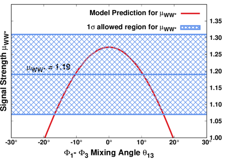
Figure 1: Variation of $\mu_{{}_{WW^{\star}}}$ with the CP-even mixing angle $\theta_{13}$ is shown with the dashed red line. The allowed shaded one sigma region for measured $\mu_{{}_{WW^{\star}}}=1.19\pm 0.12$ PDG:2020 is also shown.

We compare the total Higgs decay width in SM $\Gamma(h^{\rm SM}\to\textrm{all})\sim 4.07$ MeV Denner:2011mq ; LHCHiggsCrossSectionWorkingGroup:2013rie with the recently measured total decay width $\Gamma(h_{1}\to\textrm{all})\sim 3.2^{+2.8}_{-2.2}$ MeV at the LHC PDG:2020 . Assuming, that the model can account for the measured value of the total decay width, we constrain the model parameters by examining the bounds on the partial decay widths of decay channels for 125 GeV $h_{1}$ at LHC. To this end, we define the signal strength $\mu_{{}_{XY}}$ w.r.t. $h_{1}$ production via dominant gluon fusion in $p-p$ collision, followed by its decay to $X\ \&\ Y$ pairs in the narrow width approximation as

$$\mu_{{}_{XY}} = \frac{\sigma(pp\to h_{1}\to XY)}{\sigma(pp\to h\to XY)^{\textrm{SM}}}=\frac{\Gamma\left(h_{1}\to g\,g\right)}{\Gamma\left(h^{SM}\to g\,g\right)}\,\,\,\,\frac{\textrm{BR}\left(h_{1}\to X\,Y\right)}{\textrm{BR}\left(h^{\rm SM}\to X\,Y\right)}$$ (25)

$$= \cos^{4}\theta_{13}\,\,\frac{\Gamma(h^{\rm SM}\to\textrm{all})}{\Gamma(h_{1}\to\textrm{all})}$$

We first analyse the partial decay width of $h_{1}\to W\,W^{\star}$ channel which solely depends on $\theta_{13}$:

$$\Gamma(h_{1}\to WW^{\star}) = \cos^{2}\theta_{13}\ \Gamma(h^{\rm SM}\to WW^{\star})$$ (26)

Among the signal strengths for Higgs decaying to gauge Bosons at tree level, $\mu_{WW^{\star}}\sim 1.19\pm 0.12$ PDG:2020 has the least uncertainty for which it can provide the strongest upper bound on the mixing angle $\theta_{13}$. In figure 1, we show the one sigma band around the central value of the $\mu_{WW^{\star}}$ which restricts the model contribution curve drawn in green for $\left|\theta_{13}\right|\lesssim 10^{\circ}$ at 1 $\sigma$ level.

Next, we calculate the partial decay widths generated at one loop for $h_{1}\to\gamma\,\gamma$ and $h_{1}\to Z\,\gamma$ respectively. The contribution of charged scalars $H^{\pm}$ and vector-like leptons $\chi^{-}$ modify the SM predictions for the branching ratios. The partial decay widths for $\gamma\,\gamma$ and $Z\,\gamma$ in the model are parameterised as

$$\Gamma(h_{1}\to\gamma\,\gamma) = \cos^{2}\theta_{13}\left|1+\zeta_{\gamma\gamma}\right|^{2}\,\Gamma\left(h^{\rm SM}\to\gamma\,\gamma\right)$$ (27a)

$$\Gamma(h_{1}\to Z\,\gamma) = \cos^{2}\theta_{13}\left|1+\zeta_{Z\gamma}\right|^{2}\,\Gamma\left(h^{\rm SM}\to Z\,\gamma\right)$$ (27b)

where the SM Higgs partial decay widths in $\gamma\,\gamma$ and $Z\,\gamma$ channels are given as

$$\Gamma(h^{\rm SM}\to\gamma\gamma) = \frac{G_{F}\alpha^{2}\ m_{h}^{3}}{128\sqrt{2}\pi^{3}}\ \left|\frac{4}{3}{\cal M}^{\gamma\gamma}_{1/2}\bigg{(}\frac{4m_{t}^{2}}{m_{h}^{2}}\bigg{)}+{\cal M}^{\gamma\gamma}_{1}\bigg{(}\frac{4m_{\rm W}^{2}}{m_{h}^{2}}\bigg{)}\right|^{2}$$ (28a)

$$\Gamma(h^{\rm SM}\rightarrow Z\gamma) = \frac{G^{2}_{F}\ \alpha\,m_{W}^{2}\,m_{h}^{3}}{64\,\pi^{4}}\left(1-\frac{m_{Z}^{2}}{m_{h}^{2}}\right)^{3}\left|2\frac{\left(1-\frac{8}{3}s^{2}_{W}\right)}{c_{W}}{\cal M}^{Z\gamma}_{1/2}\left(\frac{4m_{t}^{2}}{m_{h}^{2}},\frac{4m_{t}^{2}}{m_{Z}^{2}}\right)+{\cal M}^{Z\gamma}_{1}\left(\frac{4m_{W}^{2}}{m_{h}^{2}},\frac{4m_{W}^{2}}{m_{Z}^{2}}\right)\right|^{2}$$

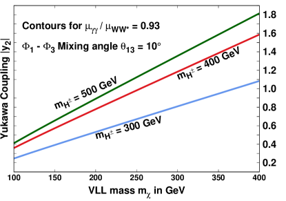
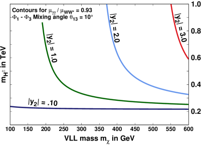
(a)

(b)

Figure 2: Contours satisfying the constraint $\mu_{{}_{\gamma\gamma}}/\mu_{{}_{WW^{\star}}}=0.93^{+0.17}_{-0.16}$ PDG:2020 for $\theta_{13}=10^{\circ}$ are drawn in (a) $m_{\chi}-\left|y_{2}\right|$ plane corresponding to three choices of charged Higgs mass and (b) $m_{\chi}-m_{H^{\pm}}$ plane corresponding to four choices of $\left|y_{2}\right|$.

The dimensionless parameters $\zeta_{\gamma\gamma}$ and $\zeta_{Z\gamma}$ are defined as

$$\zeta_{\gamma\gamma} = \frac{v_{\rm SM}}{\cos\theta_{13}}\left[\frac{\frac{g_{h_{1}H^{+}H^{-}}}{2\,m^{2}_{H^{\pm}}}{\cal M}^{\gamma\gamma}_{0}\left(\frac{4m_{H^{\pm}}^{2}}{m_{h_{1}}^{2}}\right)+\frac{y_{2}}{\sqrt{2}m_{\chi}}\sin\theta_{13}{\cal M}^{\gamma\gamma}_{1/2}\left(\frac{4\,m_{\chi}^{2}}{m_{h_{1}}^{2}}\right)}{{\cal M}^{\gamma\gamma}_{1}\left(\frac{4\,m_{\rm W}^{2}}{m_{h_{1}}^{2}}\right)+\frac{4}{3}\,{\cal M}^{\gamma\gamma}_{1/2}\left(\frac{4\,m_{t}^{2}}{m_{h_{1}}^{2}}\right)}\right]$$ (29a)

$$\zeta_{Z\gamma} = \frac{v_{\rm SM}}{\cos\theta_{13}}\left[\frac{-\,\frac{g_{h_{1}H^{+}H^{-}}}{2m_{H^{\pm}}^{2}}\,\frac{1-2s^{2}_{\theta_{W}}}{c_{\theta_{W}}}{\cal M}^{Z\gamma}_{0}\left(\frac{4m_{H^{\pm}}^{2}}{m_{h_{1}}^{2}},\frac{4m_{H^{\pm}}^{2}}{m_{Z}^{2}}\right)\ -\ \frac{y_{2}}{\sqrt{2}m_{\chi}}\ \sin\theta_{13}\ \frac{4\ s^{2}_{W}}{c_{W}}\,{\cal M}^{Z\gamma}_{1/2}\left(\frac{4m_{\chi}^{2}}{m_{h_{1}}^{2}},\frac{4m_{\chi}^{2}}{m_{Z}^{2}}\right)}{2\frac{\left(1-\frac{8}{3}s^{2}_{W}\right)}{c_{W}}{\cal M}^{Z\gamma}_{1/2}\left(\frac{4m_{t}^{2}}{m_{h_{1}}^{2}},\frac{4m_{t}^{2}}{m_{Z}^{2}}\right)+{\cal M}^{Z\gamma}_{1}\left(\frac{4m_{W}^{2}}{m_{h_{1}}^{2}},\frac{4m_{W}^{2}}{m_{Z}^{2}}\right)}\right]$$

where the triple scalar coupling $g_{h_{1}H^{+}H^{-}}=\left(v_{\rm SM}\,\lambda_{3}\,\cos\theta_{13}+v_{s}\,\lambda_{13}\,\sin\theta_{13}\right)$. The form factors ${\cal M}^{\gamma\gamma}_{0,\,1/2,\,1}$ and ${\cal M}^{Z\gamma}_{0,\,1/2,\,1}$ are defined in the appendix B. The analytical expressions for the partial widths except the additional contribution from VLL are identical to that given in the reference Bonilla:2014xba .

Using the analytical expressions for the partial decay widths for $h_{1}\to\gamma\,\gamma$, $h_{1}\to Z\,\gamma$ and $h_{1}\to W\,W^{\star}$ in equations (27a), (27b) and (26) respectively, we consider the two ratios of the signal strengths namely,

$$\frac{\mu_{{}_{\gamma\gamma}}}{\mu_{{}_{W\,W^{\star}}}} = \frac{\Gamma(h_{1}\to\gamma\,\gamma)}{\Gamma(h_{1}\to W\,W^{\star})}\times\frac{\Gamma(h^{\rm SM}\to WW^{\star})}{\Gamma(h^{\rm SM}\to\gamma\,\gamma)}=\left|1+\zeta_{\gamma\gamma}\right|^{2}$$ (30a)

$$\frac{\mu_{{}_{Z\,\gamma}}}{\mu_{{}_{W\,W^{\star}}}} = \frac{\Gamma(h_{1}\to Z\,\gamma)}{\Gamma(h_{1}\to W\,W^{\star})}\times\frac{\Gamma(h^{\rm SM}\to W\,W^{\star})}{\Gamma(h^{\rm SM}\to Z\,\gamma)}=\left|1+\zeta_{Z\gamma}\right|^{2}$$ (30b)

The experimental limits on $\mu_{{}_{\gamma\gamma}}=1.11^{+0.10}_{-0.09}$ and $\mu_{{}_{WW^{\star}}}=1.19\pm 0.12$ for $m_{h^{\rm SM}}=125.09$ GeV PDG:2020 are then substituted in equations (30a) to constrain the allowed parameter space for the Charged Higgs and singlet vector like lepton respectively. Since experimental uncertainty for $\mu_{{}_{Z\gamma}}<6.6$ PDG:2020 is large, we do not constrain the model parameters from $h_{1}\to Z\,\gamma$ decay channel.

We depict the contours satisfying $\mu_{\gamma\gamma}/\mu_{WW^{\star}}=0.93^{+0.17}_{-0.16}$ for $\theta_{13}=10^{\circ}$ in figure 2. In figure 2 contours satisfying the central value of the ratio are drawn in the $m_{\chi}-\left|y_{2}\right|$ plane for $m_{H^{\pm}}$ = 300, 400 and 500 GeV. The sensitivity of the charged Higgs mass are studied w.r.t. variation of the VLL mass from the contours satisfying the central value of the ratio in figure 2 for four choices of Yukawa couplings $\left|y_{2}\right|$ varying between 0.1 and the perturbative limit $\sqrt{4\pi}$.

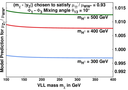
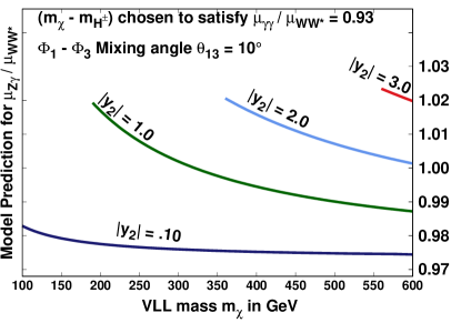
(a)

(b)

Figure 3: Variation of the ratio $\mu_{Z\gamma}/\mu_{WW^{\star}}$ with varying $m_{\chi}$ for $\theta_{13}=10^{\circ}$. The values of $\left(m_{\chi},\,\left|y_{2}\right|\right)$ in figure (a) and that of $\left(m_{\chi},\,m_{H^{\pm}}\right)$ in figure (b) are such that they satisfy the constraint $\mu_{\gamma\gamma}/\mu_{WW^{\star}}=0.93^{+0.17}_{-0.16}$ PDG:2020 as depicted in figures 2 and 2 respectively.

With the constrained parameter space from $\mu_{\gamma\gamma}$ and $\mu_{WW^{\star}}$, we estimate the ratio of signal strengths $\mu_{Z\gamma}/\mu_{WW^{\star}}$ and make a prediction for the future improved measurements with higher luminosity and kinematic reach at FCC-hh. In figure 3 we study the variation of the ratio $\mu_{Z\gamma}/\mu_{WW^{\star}}$ with varying $m_{\chi}$ for fixed $\theta_{13}=10^{\circ}$. The curves in figure 3 are depicted using those $\left(m_{\chi},\,\left|y_{2}\right|\right)$ values which satisfy the constraint $\mu_{\gamma\gamma}/\mu_{WW^{\star}}=0.93^{+0.17}_{-0.16}$ as shown in the figure 2 corresponding to $m_{H^{\pm}}$ = 300, 400 and 500 GeV respectively. Similarly, the graphs in figure 3 are depicted using those $\left(m_{\chi},\,m_{H^{\pm}}\right)$ values which satisfy the constraint $\mu_{\gamma\gamma}/\mu_{WW^{\star}}=0.93^{+0.17}_{-0.16}$ as shown in the figure 2 corresponding to $\left|y_{2}\right|$ = 0.1, 1,0, 2.0 and 3.0 respectively.

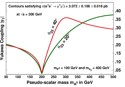
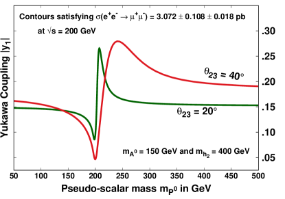
(a) $m_{P^{0}}=100\ GeV,\ m_{h_{2}}=400\ GeV.$

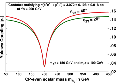
(b) $m_{A^{0}}=150\ GeV,\ m_{h_{2}}=400\ GeV.$

(c) $m_{A^{0}}=150\ GeV,\ m_{P^{0}}=100\ GeV.$

Figure 4: Contours in the plane defined by scalar/ pseudo-scalar mass and its coupling $\left|y_{1}\right|$ with SM leptons satisfying the combined analysis of DELPHI and L3 $\sigma(e^{+}\ e^{-}\to\mu^{+}\ \mu^{-})=3.072\pm 0.108\pm 0.018$ pb at $\sqrt{s}=200\ GeV$ Schael:2013ita for three benchmark points corresponding to two choices of the mixing angle $\theta_{23}$ = 20^∘ and 40^∘ respectively. The parameter space lying above the contour are forbidden by LEP observations.

3.2 LEP II Data

We validate the model from the existing LEP II data and put the lower mass bounds on the scalar and pseudo-scalar mass eigenstates. This can be achieved either by investigating the (a) direct pair production of scalars and pseudo-scalars or (b) by production of pair of fermions mediated by these additional exotic physical scalars or pesudo-scalars. VLL below 100 GeV cannot be constrained by LEP experiment as they do not couple to SM particles except $h_{1}$ (SM Like Higgs) at tree level and therefore the cross-section is expected to be highly suppressed due to the electron Yukawa coupling.

The dominant direct pair production channels at $e^{+}e^{-}$ collider:

$$e^{+}\ e^{-} \to \gamma^{\star}/\,Z^{\star}\to H^{+}+H^{-}$$ (31)

$${\rm and}\hskip 14.22636pte^{+}\ e^{-} \to Z^{\star}\to A^{0}/P^{0}+h_{i}$$ (32)

have been studied to put the lower mass bounds on $m_{H^{\pm}}\>\raisebox{-2.15277pt}{$\stackrel{{\scriptstyle\textstyle>}}{{\sim}}$}\>$ 93.5 GeV and $\sum m_{h_{i}}\>\raisebox{-2.15277pt}{$\stackrel{{\scriptstyle\textstyle>}}{{\sim}}$}\>200$ GeV Schael:2013ita .

We compute the cross-section for $e^{+}\ e^{-}\to\mu^{+}\ \mu^{-}$ from the combined analysis at LEP II which is found to be $\sigma(e^{+}\ e^{-}\to\mu^{+}\ \mu^{-})=3.072\pm 0.108\pm 0.018\ pb$ at $\sqrt{s}=200\ GeV$.

The additional contribution to $\mu$-pair production cross-section in our model can be written as:

$$\sigma_{\mu^{+}\mu^{-}}^{\rm NP} \simeq \frac{s}{64\pi}\ \sqrt{\frac{1-4\frac{m_{\mu}^{2}}{s}}{1-4\frac{m_{e}^{2}}{s}}}\,y_{1}^{4}\,\left[\left\{\frac{\cos^{2}\theta_{23}}{s-m_{A^{0}}^{2}}+\frac{\sin^{2}\theta_{23}}{s-m_{P^{0}}^{2}}\right\}^{2}+\frac{1}{\left(s-m_{h_{2}}^{2}\right)^{2}}\right]$$ (33)

where we have dropped the interference terms of $h_{2}$ with $h_{1}$ and $h_{3}$ as they are suppressed by $\left(m_{e}\ m_{\mu}\right)/v_{\rm SM}^{2}$. Also, the contributions from $h_{1}$ and $h_{3}$ and their interference are suppressed by factor of $\left(m_{e}\ m_{\mu}\right)^{2}/v_{\rm SM}^{4}$ and hence have not been taken into account. The other interference terms with $\gamma^{\star}/\,Z$ vanish. The interference term among scalars and pseudo-scalars vanish.

We compare the measured cross-section from the combined analysis of DELPHI and L3 at LEP II $\sigma(e^{+}\ e^{-}\to\mu^{+}\ \mu^{-})=3.072\pm 0.108\pm 0.018$ pb at $\sqrt{s}=200\ GeV$ Schael:2013ita with the model contribution as calculated in equation (33) for three benchmark points of the parameter space. For each such bench mark point we plot two contours corresponding to the mixing angle $\theta_{23}=10^{\circ}$ and 40^∘ respectively in (a) $m_{A^{0}}-\left|y_{1}\right|$ plane, (b) $m_{P^{0}}-\left|y_{1}\right|$ plane and (c) $m_{h_{2}}-\left|y_{1}\right|$ plane in figures 4, 4 and 4 respectively. The parameter space below the respective contour is allowed from LEP measurements.

3.3 Electroweak Precision Observables

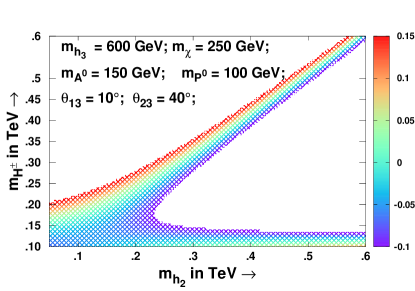
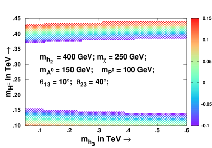
(a)

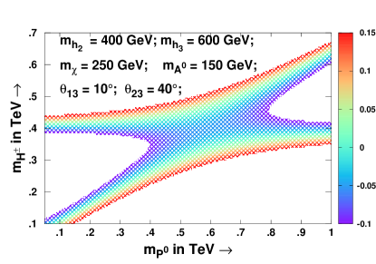
(b)

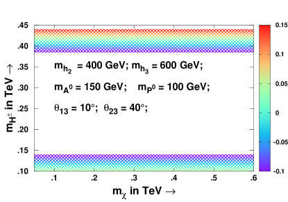
(c)

(d)

Figure 5: One sigma shaded density maps in the plane defined by respective scalar/ pseudo-scalar/ VLL masses and charged Higgs mass $m_{H^{\pm}}$ satisfying the present experimental constraint on precision variable $\Delta T=0.03\pm 0.12$ PDG:2020 .

In this subsection we compute the additional contribution to the precision observables from heavy physical mass eigenstates $m_{h_{i},\,P^{0},\,A^{0},\,\chi}>>m_{Z}$. We constrain the scalar/ pseudo-scalar masses and their mixing angles based on the available electroweak precision data. Contributions to the oblique radiative corrections are given in terms of three precision parameters known as $S$, $T$ and $U$ Peskin:1991sw ; Marciano:1990dp ; Kennedy:1990ib ; Kennedy:1991wa ; Ellis:1992zi .

The precision observables derived from the radiative corrections of the gauge Boson propagator are essentially the two point vacuum polarization tensor functions of $\Pi^{\mu\nu}_{ij}\left(q^{2}\right)$ where $q$ is the four-momentum of the vector boson ($V=W,\ Z$ or $\gamma$). Following the prescription of the reference Haber:1993wf the vacuum polarization tensor functions corresponding to pair of gauge Bosons $V_{i}-V_{j}$ can be written as

$$i\Pi^{\mu\nu}_{ij}(q) = ig^{\mu\nu}A_{ij}(q^{2})+iq^{\mu}q^{\nu}B_{ij}(q^{2})\,\,\,\,{\rm where}$$ (34a)

$$A_{ij}(q^{2}) = A_{ij}(0)+q^{2}F_{ij}(q^{2})$$ (34b)

where only $A_{ij}(q^{2})$ are the relevant functions for the computation of precision observables. The equation (34b) defines the function $F_{ij}$. Accordingly the precision parameters are defined as:

$$S \equiv \frac{1}{g^{2}}\left(16\pi\cos\theta_{W}^{2}\right)\left[F_{ZZ}(m_{Z}^{2})-F_{\gamma\gamma}(m_{Z}^{2})+\left({2\sin\theta_{W}^{2}-1\over\sin\theta_{W}\cos\theta_{W}}\right)F_{Z\gamma}(m_{Z}^{2})\right]$$ (35a)

$$T \equiv \frac{1}{\alpha_{em}}\left[{A_{WW}(0)\over m_{W}^{2}}-{A_{ZZ}(0)\over m_{Z}^{2}}\right]$$ (35b)

$$U \equiv \frac{1}{g^{2}}\left(16\pi\right)\left[F_{WW}(m_{W}^{2})-F_{\gamma\gamma}(m_{W}^{2})-{\cos\theta_{W}\over\sin\theta_{W}}F_{Z\gamma}(m_{W}^{2})\right]-S\,.$$ (35c)

where $\alpha_{em}$ is the fine structure constant. It is worthwhile to mention that although $A_{ij}(0)$ and $F_{ij}$ are divergent by themselves but the total divergence associated with each precision parameter in equations (35a), (35b) and (35c) vanish on taking into account a gauge invariant set of one loop diagrams contributing for a given pair of gauge Bosons.

The deviation from the predicted SM contribution for $S$ and $T$ parameters can be expressed analytically in terms of standard Veltman-Passarrino integrals $A_{0},\,B_{0}$ and $B_{22}$ defined in the appendix C:

$$\Delta S = \frac{G_{F}\,\alpha_{em}^{-1}}{2\sqrt{2}\,\pi^{2}}\,\sin^{2}\left(2\,\theta_{W}\right)\,\Bigg{[}\sin^{2}\theta_{13}\bigg{\{}m_{Z}^{2}\bigg{(}\mathcal{B}_{0}(m_{Z}^{2};m_{Z}^{2},m_{h_{1}}^{2})-\mathcal{B}_{0}(m_{Z}^{2};m_{Z}^{2},m_{h_{3}}^{2})\bigg{)}$$ (36a)

$$+\mathcal{B}_{22}(m_{Z}^{2};m_{Z}^{2},m_{h_{3}}^{2})-\mathcal{B}_{22}(m_{Z}^{2};m_{Z}^{2},m_{h_{1}}^{2})\bigg{\}}$$

$$+\sin^{2}\theta_{23}\bigg{(}\mathcal{B}_{22}(m_{Z}^{2};m_{h_{2}}^{2},m_{P^{0}}^{2})-\mathcal{B}_{22}(m_{Z}^{2};m_{H^{\pm}}^{2},m_{H^{\pm}}^{2})\bigg{)}\Bigg{]}$$

where

$$\mathcal{B}_{22}(q^{2};m_{1}^{2},m_{2}^{2}) \equiv B_{22}(q^{2};m_{1}^{2},m_{2}^{2})-B_{22}(0;m_{1}^{2},m_{2}^{2})$$ (36b)

$$\mathcal{B}_{0}(q^{2};m_{1}^{2},m_{2}^{2}) \equiv B_{0}(q^{2};m_{1}^{2},m_{2}^{2})-B_{0}(0;m_{1}^{2},m_{2}^{2})$$ (36c)

$$\Delta T = \frac{G_{F}\,\alpha_{em}^{-1}}{2\sqrt{2}\,\pi^{2}}\Bigg{[}\sin^{2}\theta_{13}\Bigg{\{}m_{W}^{2}\bigg{(}B_{0}(0;m_{W}^{2},m_{h_{1}}^{2})-B_{0}(0;m_{W}^{2},m_{h_{3}}^{2})\bigg{)}$$ (37)

$$-m_{Z}^{2}\bigg{(}B_{0}(0;m_{Z}^{2},m_{h_{1}}^{2})-B_{0}(0;m_{Z}^{2},m_{h_{3}}^{2})\bigg{)}+B_{22}(0;m_{W}^{2},m_{h_{3}}^{2})-B_{22}(0;m_{W}^{2},m_{h_{1}}^{2})$$

$$+B_{22}(0;m_{Z}^{2},m_{h_{1}}^{2})-B_{22}(0;m_{Z}^{2},m_{h_{3}}^{2})\Bigg{\}}-\frac{1}{2}\,A_{0}(m^{2}_{H^{\pm}})+B_{22}(0;m_{H^{\pm}}^{2},m_{h_{2}}^{2})$$

$$+\cos^{2}\theta_{23}\bigg{(}B_{22}(0;m_{H^{\pm}}^{2},m_{A^{0}}^{2})-B_{22}(0;m_{h_{2}}^{2},m_{A^{0}}^{2})\bigg{)}$$

$$+\sin^{2}\theta_{23}\bigg{(}B_{22}(0;m_{H^{\pm}}^{2},m_{P^{0}}^{2})-B_{22}(0;m_{h_{2}}^{2},m_{P^{0}}^{2})\bigg{)}$$

$$+\ 4\ \sin^{4}\theta_{W}\bigg{(}m_{\chi}^{2}\ B_{0}(0;m_{\chi}^{2},m_{\chi}^{2})-2B_{22}(0;m_{\chi}^{2},m_{\chi}^{2})\bigg{)}\Bigg{]}$$

The deviation in the theoretical predictions for precision observables in SM $\left(S_{\rm SM},\,T_{\rm SM}\right)$ from the electroweak precision measurements in the experiments for $U\neq 0$ $\left(S_{\rm expt},\,T_{\rm expt}\right)$ are parameterised as PDG:2020

$$\Delta S = S_{\rm expt.}-S_{\rm SM}=0.01\pm 0.10$$ (38a)

$$\Delta T = T_{\rm expt.}-T_{\rm SM}=0.03\pm 0.12$$ (38b)

Computing the precision observables numerically, we find that the allowed parameter space by the Higgs decays and LEP data satisfy the one sigma constraint for $\Delta S$ as given in equation (38a). In fact, the large uncertainty in the measurement allows the mass range between 50 - 1000 GeV for all scalars, pseudo-scalars and the VLL. However, the constrain on $\Delta T$ as given in equation (38b) further shrinks the allowed parameter region. We have depicted the one sigma density maps for the allowed region by the $\Delta T$ in the plane defined by the masses $m_{h_{2}}-m_{H^{\pm}}$, $m_{h_{3}}-m_{H^{\pm}}$, $m_{P^{0}}-m_{H^{\pm}}$ and $m_{\chi}-m_{H^{\pm}}$ in figure 5.

In the next section, we proceed with this constrained parameter space to look for viable explanation for the observed discrepancies in the measurements of the anomalous MDM for muon and electron.

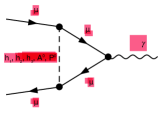
(a) Leptons

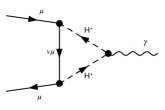
(b) Vector-like Leptons

(c) Charged Scalars

Figure 6: Dominant diagrams contributing to muon $g-2$ at one-loop level.

4 Anomalous MDM of Leptons

We compute the additional model contribution (other than SM diagrams) to the $\Delta a_{l}$ at one and two loops respectively.

In our model, the new one-loop contribution to $\Delta a_{l}$ arises from the exchange of CP-even and odd scalars and from the charged Higgs and VLL diagrams. We draw the additional (other than those allowed by SM) dominant Feynman diagrams at one loop in figure 6 based on the Lagrangian given in equations (4d), (4k) and (4l).

The sum of the contributions to lepton $\Delta a_{l}$ from the additional one-loop Feynman diagrams (other than SM) as shown in the figure 6 is calculated to be:

$$\delta a_{l}^{\rm 1\,loop} = \frac{1}{16\,\pi^{2}}\left[2\ \frac{m_{l}^{4}}{v_{\rm SM}^{2}}\ \left(\frac{\cos^{2}\theta_{13}}{m_{h_{1}}^{2}}\ +\frac{\sin^{2}\theta_{13}}{m_{h_{3}}^{2}}-\frac{1}{m_{h^{\rm SM}}^{2}}\right)\ {\cal I}_{1}+m_{l}^{2}\ \left(\frac{\cos^{2}\theta_{23}}{m_{A^{0}}^{2}}+\frac{\sin^{2}\theta_{23}}{m_{P^{0}}^{2}}\right)\ y_{1}^{2}\ {\cal I}_{2}\right.$$ (39a)

$$\left.+\frac{m_{l}^{2}}{m_{h_{2}}^{2}}\ y_{1}^{2}\ {\cal I}_{1}+\sum_{s_{i}=h_{1},h_{3},A^{0},P^{0}}\left|y_{l\chi s_{i}}\right|^{2}\ \frac{m_{l}^{2}}{m_{s_{i}}^{2}}\ {\cal I}_{3}\ +\left|y_{1}\right|^{2}\ \frac{m_{l}^{2}}{m_{H^{\pm}}^{2}}\ {\cal I}_{4}\right]$$

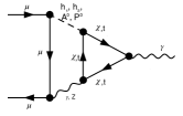
(a) Fermion triangle

(b) $H\pm$ triangle

(c) $H^{\pm}$ bubble

Figure 7: Dominant diagrams contributing to muon $g-2$ at the two-loop level.

where the one loop functions ${\cal I}_{1},\,{\cal I}_{2},\,{\cal I}_{3}$ and ${\cal I}_{4}$ are defined in the appendix D in equations (58a), (58b), (58c) and (58d) respectively.

In order to obtain the common parameter-space satisfying both $\Delta a_{\mu}$ and $\Delta a_{e}$ which are of opposite signs, it is imperative to analyse the nature of contribution by the mediating scalar/ pseudoscalar as given in figure 6. We observe that one-loop amplitudes in figure 6 are negative and positive corresponding to mediating pseudo-scalars and scalars respectively while loop amplitudes in figure 6 are positive for both pseudo-scalars and scalars except $h_{2}$ as it do not couples to VLL. The contribution from charged Higgs loop in figure 6 is negative and competitively much smaller in magnitude.

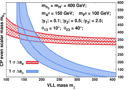
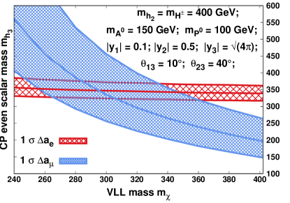
(a)

(b)

Figure 8: Colored solid contours and associated one $sigma$ bands are shown in $m_{h3}-m_{\chi}$ satisfying $\Delta a_{\mu}=\left(251\pm 59\right)\times 10^{-11}$ Muong-2:2021ojo (in blue) and $\Delta a_{e}=\left[-88\ \pm 28\,({\rm expt.})\pm 23\,(\alpha)\pm 2\,({\rm theory})\right]\times 10^{-14}$ Parker:2018vye (in red). Contours are drawn for Yukawa couplings $\left|y_{3}\right|$ = 2.5 and the perturbative limit $\sqrt{4\pi}$ in figures 8 and 8 respectively, while other physical masses, couplings and angles remain same for the both. The overlap of the two bands depict the common parameter space.

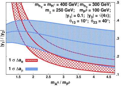
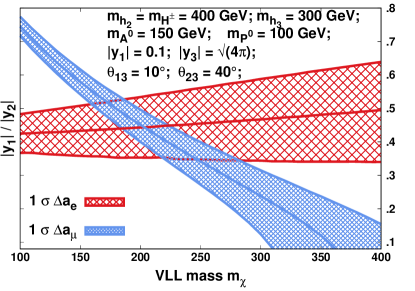
(a)

(b)

Figure 9: Colored solid contours and associated one $sigma$ bands are shown in $\left|y_{1}\right|/\left|y_{2}\right|-m_{A^{0}}/\,m_{P^{0}}$ and $\left|y_{1}\right|/\left|y_{2}\right|\,-\,m_{\chi}$ planes satisfying $\Delta a_{\mu}=\left(251\pm 59\right)\times 10^{-11}$ Muong-2:2021ojo (in blue) and $\Delta a_{e}=\left[-88\ \pm 28\,({\rm expt.})\pm 23\,(\alpha)\pm 2\,({\rm theory})\right]\times 10^{-14}$ Parker:2018vye (in red). Contours are drawn with fixed $m_{\chi}$ = 250 GeV and $m_{A^{0}}$ = 150 GeV in figures 9 and 9 respectively while other physical masses, couplings and angles remain same for the both. The overlap of the two bands depict the common parameter space.

The contributions of two loop diagrams, some of which may dominate inspite of an additional loop suppression factor play a crucial role in the estimation of anomalous MDM. It is shown in the literature that the dominant two-loop Barr-Zee diagrams mediated by neutral scalars and pseudo-scalars can become relevant for certain mass scales so that their contribution to the muon anamalous MDM are of the same order to that of one loop diagrams Chun:2020uzw .

In figure 7 we draw the dominant additional two-loop Barr-Zee diagrams (other than SM) contributing to the anomalous MDM of lepton which are based on the Lagrangian given in equations (4d), (4k) and (4l). The sum of the contributions to lepton $\Delta a_{l}$ from the additional two-loop Feynman diagrams (other than SM) as shown in the figure 7 is calculated to be:

$$\delta{a_{l}}^{2\ loop} = \frac{\alpha_{em}}{4\ \pi^{3}}\ \left[\frac{m_{l}}{v_{\rm SM}}\frac{y_{2}}{\sqrt{2}}\ \sin\theta_{13}\ \cos\theta_{13}\left\{f\left(\frac{m_{\chi}^{2}}{m_{h_{3}}^{2}}\right)-f\left(\frac{m_{\chi}^{2}}{m_{h_{1}}^{2}}\right)\right\}\right.$$

$$\left.+\frac{m_{l}}{v_{\rm SM}}\frac{m_{t}}{v_{\rm SM}}\ \left\{\sin^{2}\theta_{13}\ f\left(\frac{m_{t}^{2}}{m_{h_{3}}^{2}}\right)-\cos^{2}\theta_{13}\ f\left(\frac{m_{t}^{2}}{m_{h_{1}}^{2}}\right)+f\left(\frac{m_{t}^{2}}{m_{h^{\rm SM}}^{2}}\right)\right\}\right.$$

$$\left.+\frac{y_{1}\ y_{2}}{2}\ \frac{m_{l}}{m_{\chi}}\sin\theta_{23}\ \cos\theta_{23}\ \left\{g\left(\frac{m_{\chi}^{2}}{m_{A^{0}}^{2}}\right)-g\left(\frac{m_{\chi}^{2}}{m_{P^{0}}^{2}}\right)\right\}\right.$$

$$\left.-\frac{m_{l}^{2}}{4}\ \frac{m_{l}}{v_{\rm SM}^{2}}\left\{\frac{\cos\theta_{13}}{m_{h_{1}}^{2}}\ g_{h_{1}H^{+}H^{-}}\ \tilde{f}\left(\frac{m_{H^{\pm}}^{2}}{m_{h_{1}}^{2}}\right)-\frac{\sin\theta_{13}}{m_{h_{3}}^{2}}\ g_{h_{3}H^{+}H^{-}}\ \tilde{f}\left(\frac{m_{H^{\pm}}^{2}}{m_{h_{3}}^{2}}\right)\right\}\right]$$

where the two loop functions $f$, $g$ and $\tilde{f}$ are defined in the appendix D in equations (59a), (59b) and (59c) respectively.

We find that the two loop amplitudes with VLL triangle in figure 7 are negative for mediating scalars and positive for mediating pseudo-scalars. The two-loop contributions of the charged Higgs in figure 7 and 7 are comparatively small and negative. The dominant Barr-Zee contributions are found to depend on the mixing angle $\theta_{23}$, relative mass squared difference of the CP-odd scalars $m^{2}_{A^{0}}-m^{2}_{P^{0}}$ and the Yukawa couplings $y_{1},\,y_{2}$.

The total contribution from one and two loop diagrams are computed for the constrained parameter space. Fixing the physical masses $m_{H^{\pm}}\,=\,m_{h_{2}}$ = 400 GeV, Yukawa coupling $\left|y_{1}\right|$ = 0.1, $\Phi_{1}-\Phi_{3}$ mixing angle $\theta_{13}$ at 10^∘ and $\Phi_{2}-\Phi_{3}$ mixing angle $\theta_{23}$ at 40^∘ for our analysis, we vary $m_{h_{3}},\,m_{\chi},\,m_{A^{0}}$, $\left|y_{2}\right|$ and $\left|y_{3}\right|$ to account for the contribution to anomalous MDM as observed in the experiments. Contours fulfilling the central value for $\Delta a_{\mu}$ Muong-2:2021ojo and $\Delta a_{e}$ Parker:2018vye quoted in equations (2) and (3) respectively are depicted in $m_{\chi}-m_{h_{3}}$ plane as shown in figure 8 for $\left|y_{3}\right|$ = 2.5 and in figure 8 for the maximum allowed value of $\left|y_{3}\right|$ = $\sqrt{4\pi}$ respectively. The overlapping region of the allowed one sigma bands for $\Delta a_{\mu}$ in blue and $\Delta a_{e}$ in red exhibit the common parameter space satisfying both the experimental observations simultaneously. It is observed that overlapping region broadens for the large Yukawa coupling $\left|y_{3}\right|$ corresponding to a narrow mass range for $m_{h_{3}}$. In figure 9 and 9 we fix $m_{h_{3}}$ = 300 GeV, $\left|y_{3}\right|=\sqrt{4\pi}$ and depict the one sigma band of contours in $\left|y_{1}\right|/\left|y_{2}\right|-m_{A^{0}}/\,m_{P^{0}}$ plane for $m_{\chi}$ = 250 GeV and $\left|y_{1}\right|/\left|y_{2}\right|-m_{\chi}$ plane for $m_{A^{0}}$ = 150 GeV respectively. We observe that a common parameter space for both are possible for $m_{A^{0}}\geq 1.5\,m_{P^{0}}$ and 170 GeV $\lesssim m_{\chi}\lesssim$ 300 GeV. Choosing VLL mass at 250 GeV, $\left|y_{3}\right|=\sqrt{4\pi}$ and pseudo-scalar mass range such that $m_{A^{0}}>m_{P^{0}}$, we plot the narrow red one sigma band for $\Delta a_{e}$ contours in $m_{h_{3}}-\left(m_{A^{0}}/\,m_{P^{0}}\right)$ plane in figure 10 and observe that it completely overlaps with the broad blue one sigma band for $\Delta a_{\mu}$ contours. This constrains the $m_{h_{3}}$ to be $<$ 350 GeV.

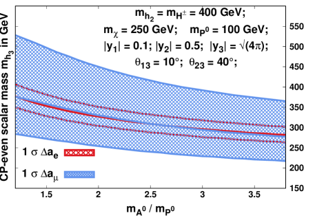
Figure 10: Colored solid contours and associated one $sigma$ bands are shown in $m_{h_{3}}-m_{A^{0}}/m_{P^{0}}$ plane satisfying $\Delta a_{\mu}=\left(251\pm 59\right)\times 10^{-11}$ Muong-2:2021ojo (in blue) and $\Delta a_{e}=\left[-88\ \pm 28\,({\rm expt.})\pm 23\,(\alpha)\pm 2\,({\rm theory})\right]\times 10^{-14}$ Parker:2018vye (in red). The overlap of the two bands depict the common parameter space.

5 Summary

In this article we considered an extended inert 2HDM model with an SM singlet complex scalar and a singlet vector like lepton field to explain the observed anomalies in the muon and electron dipole magnetic moments. The model parameters are expressed in terms of the physical masses and mixing angles of the CP even and odd scalars and are constrained from the Higgs decay to a pair of gauge Bosons at LHC, LEP data and electro-weak precision measurements. The contribution of scalars and vector-like lepton arises at the dominant one-loop and two-loop Barr-Zee diagrams. The CP even scalar one-loop contributions to $\Delta a_{l}$ are positive whereas the contribution from the CP-odd scalars is negative. The contribution of the VLL is important and decreases with the VLL mass. The Barr-Zee contributions mainly depend on the mixing angle $\theta_{23}$ and on relative mass squared difference of CP-odd scalars $A^{0}$ and $P^{0}$ and decreases with the VLL mass.

The constrained model is systematically analysed to accommodate both the experimental observations simultaneously. We depict the viable common parameter space through overlapping one sigma band of contours satisfying $\Delta a_{\mu}$ Muong-2:2021ojo and $\Delta a_{e}$ Parker:2018vye simultaneously in figures 8, 8, 9, 9 and 10. We find that there exists a fairly large common parameter space where the anomalous magnetic moments of muon and electron can be explained.

Appendix A Scalar Couplings in terms of Mass Parameters

1. Since, LHC data favours a SM-like Higgs $\sim$ 125 GeV, we allign the mass of the lightest neutral Higgs state $m_{h_{1}}$ coming predominantly from the doublet $\Phi_{1}$ with the SM Higgs $m_{h^{\rm SM}}$. In order to accomodate the $2\,\sigma$ uncertainty of the measured Higgs mass PDG:2020 the variation for $0.2\leq\lambda_{1}\leq 0.3$ may be allowed through mixing of $\Phi_{1}-{\Phi_{3}}$.

2. The quartic parameter $\lambda_{2}$ appears only in the quartic interaction of $Z_{2}$- odd particles and is therefore not constrained by our analysis.

3. Considering VEVs $v_{\rm SM}$ and $v_{s}$, mixing angles $\theta_{13}$ and $\theta_{23}$, coupling $\lambda_{13}$ and masses $m_{22}^{2},\,\,m_{h_{1}}^{2},\,\,m_{h_{2}}^{2},\,\,m_{h_{3}}^{2},\,\,m_{H^{\pm}}^{2},\,\,m_{A^{0}}^{2},\,\,{\rm and}\,\,m_{P^{0}}^{2}$ to be the free parameters, we can express $m_{11}^{2},\,\,m_{33}^{2},\,\,\lambda_{3},\,\,\lambda_{4},\,\,\lambda_{5}\,\,\lambda_{8},\,\,\lambda_{11}\,\,{\rm and}\,\,\kappa$ in terms of the above free parameters.

4. The $Z_{2}$-odd charged scalar $H^{\pm}$ comes solely from the second doublet, as in the IDM; its mass is given by

   $$m_{H^{\pm}}^{2}=\frac{1}{2}\left[-m_{22}^{2}+v_{\rm SM}^{2}\lambda_{3}+v_{s}^{2}\,\lambda_{13}\right]$$ (41)

   $\lambda_{3}$ can be expressed in terms of free parameters $\lambda_{13}$, $m_{22}^{2}$ and the charged Higgs mass as

   $$\lambda_{3}=\frac{1}{v_{\rm SM}^{2}}\left[2\,m^{2}_{H^{\pm}}+m^{2}_{22}-\lambda_{13}\,\,v_{s}^{2}\right]$$ (42)

   Notice, that the mass relations for the $Z_{2}$-odd sector from the IDM hold, namely

   $$m_{h_{2}}^{2} = m_{H^{\pm}}^{2}+\frac{v_{\rm SM}^{2}}{2}\left[\lambda_{4}+\lambda_{5}\right],$$ (43)

   $$m_{A^{0}}^{2}+m_{P^{0}}^{2} = m_{H^{\pm}}^{2}+\frac{v_{\rm SM}^{2}}{2}\left[\lambda_{4}-\lambda_{5}\right]$$ (44)

   Therefore

   $$\lambda_{4} = \frac{1}{v_{\rm SM}^{2}}\left[m_{h_{2}}^{2}+m_{A^{0}}^{2}+m_{P^{0}}^{2}-2\,m_{H^{\pm}}^{2}\right]$$ (45)

5. From pseudoscalars and heavy neutral scalar masses we have

   $$\lambda_{5}=\frac{1}{v_{\rm SM}^{2}}\left[m_{h_{2}}^{2}-m_{A^{0}}^{2}-m_{P^{0}}^{2}\right]$$ (46)

6. From mass relations for $m_{h^{0}}$ and $m_{S^{0}}$ given in equations (3.19) and (3.20) we get

   $$\lambda_{8} = \frac{1}{v_{s}^{2}}\left[m_{h_{1}}^{2}+m_{h_{3}}^{2}-\lambda_{1}\,v_{\rm SM}^{2}\right]$$ (47)

   $$\lambda_{11} = \frac{1}{v_{\rm SM}\,v_{s}}\left(\lambda_{1}\,v_{\rm SM}^{2}-\lambda_{8}\,v_{s}^{2}\right)\tan\left(2\,\theta_{13}\right)$$ (48)

7. The heavy neutral scalar mass from the Inert doublet is given as

   $$m_{h_{2}}^{2}=\frac{1}{2}\left[-m_{22}^{2}+v_{\rm SM}^{2}\lambda_{345}+v_{s}^{2}\,\lambda_{13}\right]$$ (49)

   Therefore

   $$\lambda_{13} = \frac{1}{v_{s}^{2}}\left(2\ m_{h_{2}}^{2}+m_{22}^{2}-v_{\rm SM}^{2}\lambda_{345}\right)$$ (50)

Appendix B Definition of Loop Form Factors

The loop amplitudes are expressed in terms of dimensionless parameters $\tau$ and $\lambda$, which are essentially function of the masses of physical scalars/ pseudo-scalars and fermions.

$${\cal M}^{\gamma\gamma}_{0}(\tau) = -\tau[1-\tau f(\tau)]$$ (51a)

$${\cal M}^{\gamma\gamma}_{1/2}(\tau) = 2\tau[1+(1-\tau)f(\tau)],$$ (51b)

$${\cal M}^{\gamma\gamma}_{1}(\tau) = -[2+3\tau+3\tau(2-\tau)f(\tau)]$$ (51c)

$${\cal M}^{Z\gamma}_{0}(\tau,\lambda) = I^{Z\gamma}_{1}(\tau,\lambda)$$ (51d)

$${\cal M}^{Z\gamma}_{1/2}(\tau,\lambda) = \left[I^{Z\gamma}_{1}(\tau,\lambda)-I^{Z\gamma}_{2}(\tau,\lambda)\right]$$ (51e)

$${\cal M}^{Z\gamma}_{1}(\tau,\lambda) = c_{W}\left\{4\left(3-\frac{s_{W}^{2}}{c_{W}^{2}}\right)I^{Z\gamma}_{2}(\tau,\lambda)+\left[\left(1+\frac{2}{\tau}\right)\frac{s_{W}^{2}}{c_{W}^{2}}-\left(5+\frac{2}{\tau}\right)\right]I_{1}^{Z\gamma}(\tau,\lambda)\right\}$$

with

$$f(\tau)=\left\{\begin{array}[]{cc}\arcsin^{2}\big{(}\frac{1}{\sqrt{\tau}}\big{)}&\textrm{for }\,\tau\geqslant 1,\\ -\frac{1}{4}\Big{[}\log\Big{(}\frac{1+\sqrt{1-\tau}}{1-\sqrt{1-\tau}}\Big{)}-i\pi\Big{]}^{2}&\textrm{for }\,\tau<1.\\ \end{array}\right.$$ (54)

The functions $I^{Z\gamma}_{1}$ and $I^{Z\gamma}_{2}$ are given by

$$I^{Z\gamma}_{1}(\tau,\lambda) = \frac{\tau\lambda}{2(\tau-\lambda)}+\frac{\tau^{2}\lambda^{2}}{2(\tau-\lambda)^{2}}\left[f(\tau)-f(\lambda)\right]+\frac{\tau^{2}\lambda}{(\tau-\lambda)^{2}}\left[g\left(\frac{1}{\tau}\right)-g\left(\frac{1}{\lambda}\right)\right]$$

$$I^{Z\gamma}_{2}(\tau,\lambda) = -\frac{\tau\lambda}{2(\tau-\lambda)}\left[f(\tau)-f(\lambda)\right]$$ (55)

Function $g(\tau)$ can be expressed as

$$g(\tau)=\left\{\begin{array}[]{ll}\displaystyle\sqrt{\tau^{-1}-1}\arcsin\sqrt{\tau}&\ {\rm for}\ \tau\geqslant 1\\ \displaystyle\frac{\sqrt{1-\tau^{-1}}}{2}\left[\log\frac{1+\sqrt{1-\tau^{-1}}}{1-\sqrt{1-\tau^{-1}}}-i\pi\right]&\ {\rm for}\ \tau<1\end{array}\right.$$ (56)

Appendix C Veltman Passarino Loop Integrals

The $A_{0},\,B_{0},\,B_{22}$ integrals are defined as

$$A_{0}(m^{2}) = m^{2}\ \left(\Delta+1-\ln m^{2}\right),$$ (57a)

$$B_{0}(q^{2};m_{1}^{2},m_{2}^{2}) = \Delta-\int_{0}^{1}\,dx\,\ln(X-i\epsilon)$$ (57b)

$$B_{22}(q^{2};m_{1}^{2},m_{2}^{2}) = \frac{1}{4}(\Delta+1)\left[m_{1}^{2}+m_{2}^{2}-\frac{1}{3}q^{2}\right]-\frac{1}{2}\int_{0}^{1}\,dx\,X\ln(X-i\epsilon)$$ (57c)

where $X\equiv m_{1}^{2}x+m_{2}^{2}(1-x)-q^{2}x(1-x)$ and $\Delta\equiv{2\over 4-d}+\ln(4\pi)+\gamma_{E}$ in $d$ space-time dimensions.

Appendix D One loop and two loop functions for MDM

The one loop functions ${\cal I}_{1},\,{\cal I}_{2},\,{\cal I}_{3}$ and ${\cal I}_{4}$ required to compute one loop contribution to the MDM of leptons (39a) are defined as

$${\cal I}_{1}(r^{2}) = \int_{0}^{1}dx\ \frac{(1+x)(1-x)^{2}}{(1-x)^{2}\ r^{2}+x}$$ (58a)

$${\cal I}_{2}(r^{2}) = \int_{0}^{1}dx\ \frac{-(1-x)^{3}}{(1-x)^{2}\ r^{2}+x},$$ (58b)

$${\cal I}_{3}(r^{\prime 2}) = \int_{0}^{1}dx\ \frac{x(1-x)^{2}}{(1-x)\ r^{\prime 2}+x}$$ (58c)

$$\hskip 85.35826pt{\cal I}_{4}(r^{2}) = \int_{0}^{1}dx\ \frac{-x(1-x)}{1-(1-x)\ r^{2}}$$ (58d)

with $r=\frac{m_{l}}{m_{s_{i}}},\ r^{\prime}=\frac{m_{\chi}}{m_{s_{i}}}$ and $s_{i}=h_{1},\ h_{2},\ h_{3},\ A^{0},\ P^{0}.$

The two-loop functions $f(r^{2})$, $g(r^{2})$ and $\tilde{f}(r^{2})$ contributing to the MDM of leptons given in equation (LABEL:2loopal) are defined as

$$f(r^{2}) = \frac{r^{2}}{2}\,\int_{0}^{1}dx\ \frac{1\ -\ 2x(1-x)}{x(1-x)\ -\ r^{2}}\ \ln\left[\,\frac{x(1-x)}{r^{2}}\,\right]$$ (59a)

$$g(r^{2}) = \frac{r^{2}}{2}\,\int_{0}^{1}dx\ \frac{1}{x(1-x)\ -\ r^{2}}\ \ln\left[\,\frac{x(1-x)}{r^{2}}\,\right]$$ (59b)

$$\tilde{f}(r^{2}) = \int_{0}^{1}dx\ \frac{x(1-x)}{r^{2}-\ x(1-x)}\ \ln\left[\,\frac{x(1-x)}{r^{2}}\,\right]$$ (59c)

References

- (1) A. Keshavarzi, D. Nomura and T. Teubner, Phys. Rev. D 97 (2018) no.11, 114025 doi:10.1103/PhysRevD.97.114025 [arXiv:1802.02995 [hep-ph]].
- (2) T. Blum et al. [RBC and UKQCD], Phys. Rev. Lett. 121 (2018) no.2, 022003 doi:10.1103/PhysRevLett.121.022003 [arXiv:1801.07224 [hep-lat]].
- (3) B. Abi et al. [Muon g-2], Phys. Rev. Lett. 126 (2021) no.14, 141801 doi:10.1103/PhysRevLett.126.141801 [arXiv:2104.03281 [hep-ex]].
- (4) G. W. Bennett et al. [Muon g-2], Phys. Rev. D 73 (2006), 072003 doi:10.1103/PhysRevD.73.072003 [arXiv:hep-ex/0602035 [hep-ex]].
- (5) H. N. Brown et al. [Muon g-2], Phys. Rev. Lett. 86 (2001), 2227-2231 doi:10.1103/PhysRevLett.86.2227 [arXiv:hep-ex/0102017 [hep-ex]].
- (6) T. Aoyama, N. Asmussen, M. Benayoun, J. Bijnens, T. Blum, M. Bruno, I. Caprini, C. M. Carloni Calame, M. Cè and G. Colangelo, et al. Phys. Rept. 887 (2020), 1-166 doi:10.1016/j.physrep.2020.07.006 [arXiv:2006.04822 [hep-ph]].
- (7) S. Borsanyi, Z. Fodor, J. N. Guenther, C. Hoelbling, S. D. Katz, L. Lellouch, T. Lippert, K. Miura, L. Parato and K. K. Szabo, et al. Nature 593 (2021) no.7857, 51-55 doi:10.1038/s41586-021-03418-1 [arXiv:2002.12347 [hep-lat]].
- (8) A. Crivellin, M. Hoferichter, C. A. Manzari and M. Montull, Phys. Rev. Lett. 125 (2020) no.9, 091801 doi:10.1103/PhysRevLett.125.091801 [arXiv:2003.04886 [hep-ph]].
- (9) A. Keshavarzi, W. J. Marciano, M. Passera and A. Sirlin, Phys. Rev. D 102 (2020) no.3, 033002 doi:10.1103/PhysRevD.102.033002 [arXiv:2006.12666 [hep-ph]].
- (10) G. Colangelo, M. Hoferichter and P. Stoffer, Phys. Lett. B 814 (2021), 136073 doi:10.1016/j.physletb.2021.136073 [arXiv:2010.07943 [hep-ph]].
- (11) R. H. Parker, C. Yu, W. Zhong, B. Estey and H. Müller, Science 360 (2018), 191 doi:10.1126/science.aap7706 [arXiv:1812.04130 [physics.atom-ph]].
- (12) D. Hanneke, S. Fogwell and G. Gabrielse, Phys. Rev. Lett. 100 (2008), 120801 doi:10.1103/PhysRevLett.100.120801 [arXiv:0801.1134 [physics.atom-ph]].
- (13) G. F. Giudice, P. Paradisi and M. Passera, JHEP 11 (2012), 113 doi:10.1007/JHEP11(2012)113 [arXiv:1208.6583 [hep-ph]].
- (14) H. Davoudiasl and W. J. Marciano, Phys. Rev. D 98 (2018) no.7, 075011 doi:10.1103/PhysRevD.98.075011 [arXiv:1806.10252 [hep-ph]].
- (15) X. F. Han, T. Li, L. Wang and Y. Zhang, Phys. Rev. D 99 (2019) no.9, 095034 doi:10.1103/PhysRevD.99.095034 [arXiv:1812.02449 [hep-ph]].
- (16) M. Bauer, M. Neubert, S. Renner, M. Schnubel and A. Thamm, Phys. Rev. Lett. 124 (2020) no.21, 211803 doi:10.1103/PhysRevLett.124.211803 [arXiv:1908.00008 [hep-ph]].
- (17) G. Hiller, C. Hormigos-Feliu, D. F. Litim and T. Steudtner, Phys. Rev. D 102 (2020) no.7, 071901 doi:10.1103/PhysRevD.102.071901 [arXiv:1910.14062 [hep-ph]].
- (18) C. Cornella, P. Paradisi and O. Sumensari, JHEP 01 (2020), 158 doi:10.1007/JHEP01(2020)158 [arXiv:1911.06279 [hep-ph]].
- (19) I. Bigaran and R. R. Volkas, Phys. Rev. D 102 (2020) no.7, 075037 doi:10.1103/PhysRevD.102.075037 [arXiv:2002.12544 [hep-ph]].
- (20) S. Jana, V. P. K. and S. Saad, Phys. Rev. D 101 (2020) no.11, 115037 doi:10.1103/PhysRevD.101.115037 [arXiv:2003.03386 [hep-ph]].
- (21) L. Calibbi, M. L. López-Ibáñez, A. Melis and O. Vives, JHEP 06 (2020), 087 doi:10.1007/JHEP06(2020)087 [arXiv:2003.06633 [hep-ph]].
- (22) B. Dutta, S. Ghosh and T. Li, Phys. Rev. D 102 (2020) no.5, 055017 doi:10.1103/PhysRevD.102.055017 [arXiv:2006.01319 [hep-ph]].
- (23) K. F. Chen, C. W. Chiang and K. Yagyu, JHEP 09 (2020), 119 doi:10.1007/JHEP09(2020)119 [arXiv:2006.07929 [hep-ph]].
- (24) I. Doršner, S. Fajfer and S. Saad, Phys. Rev. D 102 (2020) no.7, 075007 doi:10.1103/PhysRevD.102.075007 [arXiv:2006.11624 [hep-ph]].
- (25) T. Han, S. K. Kang and J. Sayre, JHEP 02 (2016), 097 doi:10.1007/JHEP02(2016)097 [arXiv:1511.05162 [hep-ph]].
- (26) G. Aad et al. [ATLAS], [arXiv:2007.07830 [hep-ex]].
- (27) A. E. Cárcamo Hernández, Y. Hidalgo Velásquez, S. Kovalenko, H. N. Long, N. A. Pérez-Julve and V. V. Vien, [arXiv:2002.07347 [hep-ph]].
- (28) M. Badziak and K. Sakurai, JHEP 10 (2019), 024 doi:10.1007/JHEP10(2019)024 [arXiv:1908.03607 [hep-ph]].
- (29) M. Endo and W. Yin, JHEP 08 (2019), 122 doi:10.1007/JHEP08(2019)122 [arXiv:1906.08768 [hep-ph]].
- (30) F. J. Botella, F. Cornet-Gomez and M. Nebot, Phys. Rev. D 102 (2020) no.3, 035023 doi:10.1103/PhysRevD.102.035023 [arXiv:2006.01934 [hep-ph]].
- (31) E. Coluccio Leskow, G. D’Ambrosio, A. Crivellin and D. Müller, Phys. Rev. D 95 (2017) no.5, 055018 doi:10.1103/PhysRevD.95.055018 [arXiv:1612.06858 [hep-ph]].
- (32) A. Crivellin, D. Mueller and F. Saturnino, Phys. Rev. Lett. 127 (2021) no.2, 021801 doi:10.1103/PhysRevLett.127.021801 [arXiv:2008.02643 [hep-ph]].
- (33) E. J. Chun and J. Kim, JHEP 07 (2016), 110 doi:10.1007/JHEP07(2016)110 [arXiv:1605.06298 [hep-ph]].
- (34) A. Cherchiglia, D. Stöckinger and H. Stöckinger-Kim, Phys. Rev. D 98 (2018), 035001 doi:10.1103/PhysRevD.98.035001 [arXiv:1711.11567 [hep-ph]].
- (35) S. D. Thomas and J. D. Wells, Phys. Rev. Lett. 81 (1998), 34-37 doi:10.1103/PhysRevLett.81.34 [arXiv:hep-ph/9804359 [hep-ph]].
- (36) B. Barman, D. Borah, L. Mukherjee and S. Nandi, Phys. Rev. D 100 (2019) no.11, 115010 doi:10.1103/PhysRevD.100.115010 [arXiv:1808.06639 [hep-ph]].
- (37) R. Dermisek and A. Raval, Phys. Rev. D 88 (2013), 013017 doi:10.1103/PhysRevD.88.013017 [arXiv:1305.3522 [hep-ph]].
- (38) A. Falkowski, D. M. Straub and A. Vicente, JHEP 05 (2014), 092 doi:10.1007/JHEP05(2014)092 [arXiv:1312.5329 [hep-ph]].
- (39) A. Crivellin and M. Hoferichter, JHEP 07 (2021), 135 doi:10.1007/JHEP07(2021)135 [arXiv:2104.03202 [hep-ph]].
- (40) J. Liu, C. E. M. Wagner and X. P. Wang, JHEP 03 (2019), 008 doi:10.1007/JHEP03(2019)008 [arXiv:1810.11028 [hep-ph]].
- (41) M. Abdullah, B. Dutta, S. Ghosh and T. Li, Phys. Rev. D 100 (2019) no.11, 115006 doi:10.1103/PhysRevD.100.115006 [arXiv:1907.08109 [hep-ph]].
- (42) C. Arbeláez, R. Cepedello, R. M. Fonseca and M. Hirsch, Phys. Rev. D 102 (2020) no.7, 075005 doi:10.1103/PhysRevD.102.075005 [arXiv:2007.11007 [hep-ph]].
- (43) N. Haba, Y. Shimizu and T. Yamada, PTEP 2020 (2020) no.9, 093B05 doi:10.1093/ptep/ptaa098 [arXiv:2002.10230 [hep-ph]].
- (44) J. L. Yang, T. F. Feng and H. B. Zhang, J. Phys. G 47 (2020) no.5, 055004 doi:10.1088/1361-6471/ab7986 [arXiv:2003.09781 [hep-ph]].
- (45) C. Hati, J. Kriewald, J. Orloff and A. M. Teixeira, JHEP 07 (2020), 235 doi:10.1007/JHEP07(2020)235 [arXiv:2005.00028 [hep-ph]].
- (46) M. Trodden, Rev. Mod. Phys. 71 (1999), 1463-1500 doi:10.1103/RevModPhys.71.1463 [arXiv:hep-ph/9803479 [hep-ph]].
- (47) J. E. Kim, Phys. Rept. 150 (1987), 1-177 doi:10.1016/0370-1573(87)90017-2
- (48) J. M. Gerard and M. Herquet, Phys. Rev. Lett. 98 (2007), 251802 doi:10.1103/PhysRevLett.98.251802 [arXiv:hep-ph/0703051 [hep-ph]].
- (49) A. Broggio, E. J. Chun, M. Passera, K. M. Patel and S. K. Vempati, JHEP 11 (2014), 058 doi:10.1007/JHEP11(2014)058 [arXiv:1409.3199 [hep-ph]].
- (50) J. Cao, P. Wan, L. Wu and J. M. Yang, Phys. Rev. D 80 (2009), 071701 doi:10.1103/PhysRevD.80.071701 [arXiv:0909.5148 [hep-ph]].
- (51) V. Ilisie, JHEP 04 (2015), 077 doi:10.1007/JHEP04(2015)077 [arXiv:1502.04199 [hep-ph]].
- (52) T. Abe, R. Sato and K. Yagyu, JHEP 07 (2015), 064 doi:10.1007/JHEP07(2015)064 [arXiv:1504.07059 [hep-ph]].
- (53) L. Wang and X. F. Han, JHEP 05 (2015), 039 doi:10.1007/JHEP05(2015)039 [arXiv:1412.4874 [hep-ph]].
- (54) E. J. Chun, Z. Kang, M. Takeuchi and Y. L. S. Tsai, JHEP 11 (2015), 099 doi:10.1007/JHEP11(2015)099 [arXiv:1507.08067 [hep-ph]].
- (55) S. Dutta, A. Goyal and M. P. Singh, JHEP 07 (2019), 076 doi:10.1007/JHEP07(2019)076 [arXiv:1809.07877 [hep-ph]].
- (56) J. Kawamura, S. Okawa and Y. Omura, JHEP 08 (2020), 042 doi:10.1007/JHEP08(2020)042 [arXiv:2002.12534 [hep-ph]].
- (57) J. E. Chun and T. Mondal, JHEP 11 (2020), 077 doi:10.1007/JHEP11(2020)077 [arXiv:2009.08314 [hep-ph]].
- (58) Y. Amhis et al. [Heavy Flavor Averaging Group (HFAG)], [arXiv:1412.7515 [hep-ex]].
- (59) P.A. Zyla et al. (Particle Data Group), Prog. Theor. Exp. Phys. 2020, 083C01 (2020).
- (60) A. Denner, S. Heinemeyer, I. Puljak, D. Rebuzzi and M. Spira, Eur. Phys. J. C 71 (2011), 1753 doi:10.1140/epjc/s10052-011-1753-8 [arXiv:1107.5909 [hep-ph]].
- (61) S. Heinemeyer et al. [LHC Higgs Cross Section Working Group], doi:10.5170/CERN-2013-004 [arXiv:1307.1347 [hep-ph]].
- (62) C. Bonilla, D. Sokolowska, N. Darvishi, J. L. Diaz-Cruz and M. Krawczyk, J. Phys. G 43 (2016) no.6, 065001 doi:10.1088/0954-3899/43/6/065001 [arXiv:1412.8730 [hep-ph]].
- (63) S. Schael et al. [ALEPH, DELPHI, L3, OPAL and LEP Electroweak], Phys. Rept. 532 (2013), 119-244 doi:10.1016/j.physrep.2013.07.004 [arXiv:1302.3415 [hep-ex]].
- (64) M. E. Peskin and T. Takeuchi, Phys. Rev. D 46 (1992), 381-409
- (65) W. J. Marciano and J. L. Rosner, Phys. Rev. Lett. 65 (1990), 2963-2966 [erratum: Phys. Rev. Lett. 68 (1992), 898]
- (66) D. C. Kennedy and P. Langacker, Phys. Rev. Lett. 65 (1990), 2967-2970 [erratum: Phys. Rev. Lett. 66 (1991), 395]
- (67) D. C. Kennedy, Phys. Lett. B 268 (1991), 86-88
- (68) J. R. Ellis, G. L. Fogli and E. Lisi, Phys. Lett. B 285 (1992), 238-244
- (69) H. E. Haber, [arXiv:hep-ph/9306207 [hep-ph]].