Stokes traction on an active particle

Abstract

The mechanics and statistical mechanics of a suspension of active particles are determined by the traction (force per unit area) on their surfaces. Here we present an exact solution of the direct boundary integral equation for the traction on a spherical active particle in an imposed slow viscous flow. Both single- and double-layer integral operators can be simultaneously diagonalised in a basis of irreducible tensorial spherical harmonics and the solution, thus, can be presented as an infinite number of linear relations between the harmonic coefficients of the traction and the velocity at the boundary of the particle. These generalise Stokes laws for the force and torque. Using these relations we obtain simple expressions for physically relevant quantities such as the symmetric-irreducible dipole acting on, or the power dissipated by, an active particle in an arbitrary imposed flow. We further present an explicit expression for the variance of the Brownian contributions to the traction on an active colloid in a thermally fluctuating fluid.

I Introduction

A passive colloidal particle produces flow in the ambient fluid when it translates or rotates. In contrast, an active particle can produce a flow even when stationary (Paxton et al., 2004; Howse et al., 2007; Jiang et al., 2010; Ebbens and Howse, 2010; Palacci et al., 2013). Examples include microorganisms (Brennen and Winet, 1977) and autophoretic particles (Ebbens and Howse, 2010). The exterior flow of active particles is due to local non-equilibrium processes such as ciliary motion (in the case of microorganisms) and osmotic flows (in the case of autophoretic particles). These non-equilibrium processes, when confined to a thin layer at the surface of the particles, can be modelled by adding a surface slip $\text{$\boldsymbol{v}$}^{\mathcal{A}}$ to the commonly used no-slip boundary condition on particle surfaces (Lighthill, 1952; Blake, 1971a; Anderson, 1989). The surface slip sets the ambient fluid in motion, causing stresses that react back on the particle. For a rigid particle, these integrate to a net force and a net torque on the particle centre of mass. Since fluid inertia is negligible at the colloidal scale, fluid motion is governed by the Stokes equation. The solution of the Stokes equation with prescribed velocity boundary conditions provides the stress in the fluid and, when evaluated on the particle, the traction (force per unit area) (Stokes, 1850; Landau and Lifshitz, 1959; Brunn, 1976, 1979; Pak and Lauga, 2014; Pedley, 2016; Pedley et al., 2016; Rojas-Pérez et al., 2021). The boundary integral formulation of the Stokes equation provides an alternative route to obtaining the traction that obviates the need to solve for the fluid flow in the bulk (Lorentz, 1907; Odqvist, 1930; Ladyzhenskaia, 1969; Cheng and Cheng, 2005). Instead, it provides a direct linear integral relation between quantities that are defined only at the boundaries, namely the traction and the velocity boundary condition. The boundary integral formulation has been used extensively to describe the dynamics of passive colloidal particles (Youngren and Acrivos, 1975; Felderhof, 1976a, b; Zick and Homsy, 1982; Schmitz and Felderhof, 1982) and, more recently, of active colloidal particles (Ghose and Adhikari, 2014; Singh et al., 2015; Singh and Adhikari, 2017, 2018).

Despite the large body of work on the integral equation approach to active particle dynamics, the simplest problem of a single active sphere in an unbounded fluid has not been solved exactly. Apart from its intrinsic theoretical interest, such a solution is of potential use in numerical solutions of the boundary integral equation for many particles, where numerical iterations can be initialised with the exact one-particle solution. It is known that discretisations of boundary integral equations for this class of problems leads to diagonally dominant linear systems and the one-particle solution is the exact solution when hydrodynamic interactions are ignored. This suggests that iterations initialised at the one-particle solution can converge rapidly to the diagonally-dominant numerical solutions (Singh and Adhikari, 2018).

In this paper we solve the direct boundary integral equation exactly for the traction on a spherical active particle in an unbounded fluid. Expansion in a complete basis followed by the minimisation of the residual is a convenient strategy for solving linear integral equations. In this so-called Ritz-Galerkin procedure (Boyd, 2000; Finlayson and Scriven, 1966; Singh et al., 2015), a basis that yields a diagonal linear system is particularly useful as the system, then, is trivially soluble. The direct boundary integral equation contains a pair of integral operators – the single-layer and double-layer operators – and it is not obvious that a basis that diagonalises one operator will necessarily diagonalise the other. Here we show that the basis of tensorial spherical harmonics (TSH) simultaneously diagonalises both the single-layer and double-layer integral operators and, in this sense, provides the most appropriate choice of basis. The boundary integral equation is reduced, thereby, to an infinite-dimensional diagonal linear system that can be solved trivially. We obtain compact, closed-form linear relations between the harmonic modes of the traction and the boundary velocity. The first two of these are the familiar Stokes laws for the force and torque of a spherical particle of radius $b$ in rigid body motion in an unbounded fluid of dynamic viscosity $\eta$ containing the scalar friction coefficients $6\pi\eta b$ and $8\pi\eta b^{3}$, respectively (Stokes, 1850; Happel and Brenner, 1965).

In what follows, we present our solution and some implications thereof in detail. In Section II we discuss our main findings – exact linear relations between the traction and the boundary velocity on an active particle in an imposed flow in terms of scalar generalised friction coefficients. We refer to these relations as generalised Stokes laws and emphasise that the friction coefficients due to imposed flow and activity are distinct. We then turn towards their derivation in Section III. We briefly recall the boundary integral representation of Stokes flow for three distinct contributions to the traction on the surface of an active particle in an imposed flow. These are (a) rigid body motion, (b) imposed flow, and (c) active slip. Using spectral expansions and Ritz-Galerkin discretisation of the boundary integral equations we derive an exact solution thereof in terms of matrix elements of the single- and double-layer integrals. These matrix elements are found to diagonalise simultaneously in a basis of TSH. The resulting linear system of equations is thus solved trivially to find the generalised Stokes laws. In Section IV we discuss a number of applications of our findings. First, we derive an expression relating the expansion coefficients of the imposed flow, expanded in TSH on the surface of the sphere, with its Taylor expansion about the centre of the particle, and thus relate our work to the generalised Faxén relations (Brunn, 1980). We then discuss the symmetric-irreducible dipole on an active particle in an imposed straining flow. In terms of the previously derived friction coefficients we then obtain an expression for the power dissipated by an active particle. Finally, we present an explicit expression for the variance of the Brownian contributions to the traction on an active colloid in a thermally fluctuating system. We conclude in Section V by summarising our results, putting them into context with previous work, and suggesting directions for future research.

II results

In this section we briefly outline our main results for the traction on an active colloidal particle due to the most general form of surface velocity and arbitrary imposed flow $\boldsymbol{v}^{\infty}(\boldsymbol{r})$. We consider a spherical active particle of radius $b$ in an incompressible fluid of viscosity $\eta$. The boundary condition at the surface of the particle is

$$\boldsymbol{v}(\boldsymbol{R}+\boldsymbol{\rho})=\boldsymbol{V}+\boldsymbol{\Omega}\times\boldsymbol{\rho}+\boldsymbol{v}^{\mathcal{A}}(\boldsymbol{\rho})=\boldsymbol{v}^{\mathcal{D}}(\boldsymbol{\rho})+\boldsymbol{v}^{\mathcal{A}}(\boldsymbol{\rho}).$$ (1)

The rigid body motion $\boldsymbol{v}^{\mathcal{D}}$ is specified by the translational velocity $\boldsymbol{V}$ and angular velocity $\mathbf{\boldsymbol{\Omega}}$ of the particle. Here, $\boldsymbol{R}$ is the centre of the colloid, $\boldsymbol{\rho}$ is its radius vector and $\boldsymbol{v}^{\mathcal{A}}$ is its active slip velocity. The only restriction on the active slip is that it conserves mass in the fluid, ie

$$\int\hat{\boldsymbol{\rho}}\cdot\boldsymbol{v}^{\mathcal{A}}\,d\mathcal{S}=0,$$ (2)

where $\mathcal{S}$ is the surface of the colloid and $\hat{\boldsymbol{\rho}}$ is the unit normal vector to the surface of the colloid, pointing into the surrounding fluid.

It is convenient to express the traction on the particle as a sum of three distinct contributions

$$\boldsymbol{f}=\boldsymbol{f}^{\mathcal{D}}+\boldsymbol{f}^{\infty}+\boldsymbol{f}^{\mathcal{A}}.$$ (3)

Here, $\boldsymbol{f}^{\mathcal{D}}$ is the traction due to the colloid’s rigid body motion $\boldsymbol{v}^{\mathcal{D}}$ alone, $\boldsymbol{f}^{\infty}$ represents the traction on a no-slip particle when held stationary in an imposed flow $\boldsymbol{v}^{\infty}$, and $\boldsymbol{f}^{\mathcal{A}}$ is the contribution from active surface slip $\boldsymbol{v}^{\mathcal{A}}$, see Appendix A.

In order to parametrise the surface fields on the boundary of the active particle, we expand the velocity and the traction at the colloid’s surface in tensorial spherical harmonics (TSH) $\boldsymbol{Y}^{(l)}(\hat{\boldsymbol{\rho}})$ as

$$\boldsymbol{v}^{\lambda}(\boldsymbol{R}+\boldsymbol{\rho})=\sum_{l=1}^{\infty}w_{l}\boldsymbol{V}^{\lambda(l)}\odot\boldsymbol{Y}^{(l-1)}(\hat{\boldsymbol{\rho}}),\quad\boldsymbol{f}^{\lambda}(\boldsymbol{R}+\boldsymbol{\rho})=\sum_{l=1}^{\infty}\tilde{w}_{l}\boldsymbol{F}^{\lambda(l)}\odot\boldsymbol{Y}^{(l-1)}(\hat{\boldsymbol{\rho}}),$$ (4)

where $\lambda\in\left\{\mathcal{D},\infty,\mathcal{A}\right\}$, and

$$w_{l}=\frac{1}{(l-1)!(2l-3)!!},\qquad\tilde{w}_{l}=\frac{2l-1}{4\pi b^{2}}.$$ (5)

The product $\odot$ represents a maximal contraction of indices between two tensors. The TSH are defined as

$$Y_{\alpha_{1}\dots\alpha_{l}}^{(l)}(\hat{\boldsymbol{\rho}})=(2l-1)!!\Delta_{\alpha_{1}\dots\alpha_{l},\beta_{1}\dots\beta_{l}}^{(l)}\hat{\rho}_{\beta_{1}}\dots\hat{\rho}_{\beta_{l}}=(-1)^{l}\,\rho^{l+1}\,\nabla_{\alpha_{1}}\dots\nabla_{\alpha_{l}}\frac{1}{\rho},$$ (6)

with $\rho=\left\|\boldsymbol{\rho}\right\|_{2}$, where $\left\|\cdot\right\|_{2}$ is the Euclidean norm and $\boldsymbol{\Delta}{}^{(l)}$ is a rank $2l$ tensor, which projects a tensor of rank $l$ onto its symmetric and traceless part. Excellent summaries of their properties and the identities they obey are available in the literature (Brunn, 1976, 1979; Hess, 2015).

By definition, $\boldsymbol{F}^{\lambda(l)}$ and $\boldsymbol{V}^{\lambda(l)}$ are symmetric-irreducible in their last $l-1$ indices, and thus can each be expressed as the sum of three irreducible tensors, $\boldsymbol{F}^{\lambda(l\sigma)}$ and $\boldsymbol{V}^{\lambda(l\sigma)}$, with the index $\sigma\in\{s,a,t\}$ labelling the symmetric-irreducible (rank $l$), the antisymmetric (rank $l-1$), and the trace (rank $l-2$) parts of the reducible tensors, respectively (Hess, 2015). This decomposition and the projection of the expansion coefficients onto their irreducible subspaces are given by

$$\boldsymbol{F}^{\lambda(l)}=\boldsymbol{D}^{(l\sigma)}\odot\boldsymbol{F}^{\lambda(l\sigma)},\qquad\boldsymbol{F}^{\lambda(l\sigma)}=\boldsymbol{P}^{(l\sigma)}\odot\boldsymbol{F}^{\lambda(l)},$$ (7)

respectively, with analogous expressions for the velocity coefficients. Repeated mode indices $(l\sigma)$ are summed over implicitly for the decomposition operators $\boldsymbol{D}^{(l\sigma)}$. Both the decomposition operators and the projection operators are explicitly defined in Section III.3.

As derived in Sections III.2 and III.3, the generalised Stokes laws for an isolated active particle in an unbounded domain are

$$\boldsymbol{F}^{\mathcal{D}(l\sigma)}=-\gamma_{l\sigma}\,\boldsymbol{V}^{\mathcal{D}(l\sigma)},\quad\boldsymbol{F}^{\infty(l\sigma)}=\gamma_{l\sigma}\,\boldsymbol{V}^{\infty(l\sigma)},\quad\boldsymbol{F}^{\mathcal{A}(l\sigma)}=-\hat{\gamma}_{l\sigma}\,\boldsymbol{V}^{\mathcal{A}(l\sigma)},$$ (8)

for which we can give the scalar generalised friction coefficients exactly to arbitrary order in $l$ as

$$\gamma_{ls}=\frac{4\pi\eta b\,\left(2l+1\right)}{\left(l+1\right)\left(l-1\right)!\left(2l-3\right)!!}, \gamma_{la}=\frac{4\pi\eta b}{\left(l-1\right)!\left(2l-3\right)!!}, \gamma_{lt}=\frac{4\pi\eta b}{(l-2)\left(l-1\right)!\left(2l-5\right)!!},$$

$$\hat{\gamma}_{ls}=\frac{4\pi\eta b\,\left(2l^{2}+1\right)}{\left(l+1\right)\left(l-1\right)!\left(2l-1\right)!!}, \hat{\gamma}_{la}=\frac{4\pi\eta b\,\left(l+1\right)}{\left(l-1\right)!\left(2l-1\right)!!}, \hat{\gamma}_{lt}=\frac{8\pi\eta b\,l}{\left(l-1\right)!\left(2l-1\right)!!}.$$ (9)

It should be noted that while the friction coefficients due to imposed fluid flow ($\gamma_{l\sigma}$) and those due to active surface slip ($\hat{\gamma}_{l\sigma}$) are equivalent for the modes of rigid body motion, see Section IV, they are in general distinct. The difference is due to the double-layer integral in the boundary integral equations (13). The friction coefficients $\gamma_{1s}$, $\gamma_{2s}$, and $\gamma_{2a}$ are available in the literature in terms of a Taylor expansion of the imposed flow about the centre of the particle and referred to as the Faxén relations (Faxén, 1922; Batchelor and Green, 1972; Rallison, 1978). On the other hand, our results have been obtained in terms of expansion coefficients of the imposed flow for arbitrary $(l\sigma)$. We derive a relation between these two approaches in Section IV.1. More generally, analogous expressions to $\gamma_{l\sigma}$ for arbitrary modes $(l\sigma)$ have been obtained by various authors (Brunn, 1976, 1979; Felderhof, 1976a, b; Schmitz and Felderhof, 1982); see Table 1.

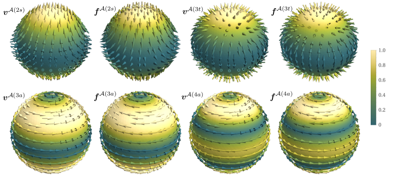
Figure 1: Panels denoted by $\boldsymbol{v}^{\mathcal{A}(l\sigma)}$ ($\boldsymbol{f}^{\mathcal{A}(l\sigma)}$) show the vector field plots of the slip (traction) due to an isolated $(l\sigma)$ mode of the expansion (4). Here, the irreducible tensors $\boldsymbol{V}^{\lambda(l\sigma)}$ are naturally parametrised in terms of the TSH as follows: $\mathbf{V}^{\lambda(ls)}=V_{ls}^{0,\lambda}\,\mathbf{Y}^{(l)}(\boldsymbol{e}),$ $\mathbf{V}^{\lambda(la)}=V_{la}^{0,\lambda}\,\mathbf{Y}^{(l-1)}(\boldsymbol{e}),$ and $\mathbf{V}^{\lambda(lt)}=V_{lt}^{0,\lambda}\,\mathbf{Y}^{(l-2)}(\boldsymbol{e}),$ where the uniaxial parameterisations are defined in terms of the orientation vector $\boldsymbol{e}$ of the active particle and $V_{l\sigma}^{0,\lambda}$ are the scalar strengths of the modes. From this parametrisation, it follows that the $\mathbf{V}^{\lambda(l\sigma)}$ are either even (apolar) or odd (polar) under inversion symmetry $\boldsymbol{e}\rightarrow-\boldsymbol{e}$ with respect to the orientation of the particle. The figure shows the vector fields $\boldsymbol{v}^{\mathcal{A}}$ and $\boldsymbol{f}^{\mathcal{A}}$ due to the leading modes of apolar $(2s)$, polar $(3t)$, achiral $(3a)$, and chiral $(4a)$ symmetry. The fields have been plotted on the surface of the particle with orientation $\boldsymbol{e}$ along the north pole. For clarity, we have lifted the vector field off the surface slightly, while its magnitude has been overlaid on the surface. It follows directly from the scalar friction coefficients of the generalised Stokes laws (8) that both slip and traction exhibit the same symmetry.

	Boundary condition	Expansion basis	Methodology
Stokes (Stokes, 1850)	No-slip (passive)
Lighthill (Lighthill, 1952) and Blake (Blake, 1971a)	Axisymmetric slip (active)	Scalar harmonics	Lamb’s general solution and scalar harmonic expansion of boundary condition to obtain coefficients of the expansion
Felderhof and Schmitz (Felderhof, 1976a, b; Schmitz and Felderhof, 1982)	Mixed slip-stick (passive) in imposed flow	Vector spherical harmonics (VSH)	BIE for a passive no-slip sphere. Single-layer diagonalises under VSH (Antenna theorems), obtained $\gamma$
Brunn (Brunn, 1976, 1979)	Mixed slip-stick (passive) in imposed flow	Tensor spherical harmonics (TSH)	Lamb’s general solution in terms of multipole potentials, using boundary conditions to find coefficients, obtained $\gamma$
Ghose and Adhikari (Ghose and Adhikari, 2014)	General slip	TSH	Indirect formulation of the BIE. Friction tensors for the first few modes.
Pak and Lauga (Pak and Lauga, 2014), Pedley et al (Pedley, 2016; Pedley et al., 2016)	General slip	Scalar harmonics	Extend Lighthill and Blake’s calculation to include azimuthal slip using Lamb’s general solution
This paper	General slip	TSH	Direct formulation of the BIE, introduced in (Singh et al., 2015; Singh and Adhikari, 2018). Friction tensors for all modes due to slip and imposed flow.

Table 1: Chronology of analytical results for the traction on a single spherical particle in an unbounded Stokes flow. Here “active” implies a sphere with active surface slip, while “passive” implies a sphere with no-slip, or alternatively a slip-stick boundary condition. In the latter, passive case, slip must be interpreted as a passive feature, comparable to the slippage at a boundary of the fluid domain (Barrat, 1999; Lauga and Squires, 2005; Ketzetzi et al., 2020). The two main approaches to obtain higher order friction coefficients are (a) using Lamb’s general solution to obtain the flow field around a particle, from which the stress tensor and thus the traction can be derived, and (b) solving the boundary integral equation (BIE) to obtain the traction directly.

It is intuitive that in the unbounded domain the generalised Stokes laws, expressing the linear relations between the irreducible modes of the traction and the corresponding modes of the boundary velocity, must be scalar relations due to symmetry considerations. A visualisation of this in terms of the active slip velocity and the resulting hydrodynamic traction due to a given ($l\sigma$) mode is shown in Figure 1.

III Derivation

This section is dedicated to the derivation of the generalised Stokes laws, Eq. (8). We revisit the boundary integral formulation of the Stokes equation and define the linearly independent boundary integral equations for the contributions to the force per unit area (traction) on the particle due to (a) rigid body motion, (b) imposed flow, and (c) active slip. We then solve these boundary integral equations exactly, using spectral expansions and Ritz-Galerkin discretisation. The matrix elements of the resulting linear system of equations are solved for in Fourier space, and found to diagonalise simultaneously in a basis of tensorial spherical harmonics. This diagonalisation results directly in the generalised Stokes laws.

III.1 Boundary integral formulation of the Stokes equation

We recall the boundary integral equation for a particle with boundary conditions given by Eq. (1) in an imposed flow $\boldsymbol{v}^{\infty}(\boldsymbol{r})$. Incompressibility of the fluid implies $\boldsymbol{\nabla}\cdot\boldsymbol{v}=0$. At the colloidal scale, the fluid satisfies the Stokes equation, $\boldsymbol{\nabla}\cdot\boldsymbol{\sigma}=0$, with the Cauchy stress tensor $\sigma_{\alpha\beta}=-p\delta_{\alpha\beta}+\eta\left(\nabla_{\alpha}v_{\beta}+\nabla_{\beta}v_{\alpha}\right)$, where $p$ is the fluid pressure and $\boldsymbol{\delta}$ is the Kronecker-delta. The boundary integral representation of the Stokes equation is then used to write the flow produced by an active particle in an imposed velocity field $\boldsymbol{v}^{\infty}(\boldsymbol{r})$ (Lorentz, 1907; Odqvist, 1930; Ladyzhenskaia, 1969; Youngren and Acrivos, 1975; Zick and Homsy, 1982; Muldowney and Higdon, 1995; Pozrikidis, 1992; Cheng and Cheng, 2005; Leal, 2007; Singh et al., 2015), using the Einstein summation convention for repeated Cartesian indices,

$$v_{\alpha}(\boldsymbol{r}) =v_{\alpha}^{\infty}(\boldsymbol{r})-\int G_{\alpha\beta}(\boldsymbol{r},\boldsymbol{r}^{\prime})f_{\beta}(\boldsymbol{r}^{\prime})\,d\mathcal{S}+\int K_{\beta\alpha\nu}(\boldsymbol{r}^{\prime},\boldsymbol{r})\hat{\rho}_{\nu}^{\prime}v_{\beta}(\boldsymbol{r}^{\prime})\,d\mathcal{S},\qquad\boldsymbol{r}\in\mathcal{V},\quad\boldsymbol{r}^{\prime}=\boldsymbol{R}+\boldsymbol{\rho}^{\prime}\in\mathcal{S}.$$ (10)

An outline of the derivation of this classical result is presented in Appendix A in the notation of this paper. In the above, $\mathcal{V}$ indicates the volume of the surrounding fluid. The integral kernels for the fluid velocity are the Green’s function $\boldsymbol{G}$ of Stokes flow and the stress tensor $\boldsymbol{K}$ associated with it. Together with the pressure field $\boldsymbol{P}$ they satisfy (Pozrikidis, 1992)

$$\nabla_{\alpha}G_{\alpha\beta}(\boldsymbol{r},\boldsymbol{r}^{\prime})=0,\quad-\nabla_{\alpha}P_{\beta}(\boldsymbol{r},\boldsymbol{r}^{\prime})+\eta\nabla^{2}G_{\alpha\beta}(\boldsymbol{r},\boldsymbol{r}^{\prime})=-\delta(\boldsymbol{r}-\boldsymbol{r}^{\prime})\delta_{\alpha\beta},$$

$$K_{\alpha\beta\nu}(\boldsymbol{r},\boldsymbol{r}^{\prime})=-\delta_{\alpha\nu}P_{\beta}(\boldsymbol{r},\boldsymbol{r}^{\prime})+\eta\left[\nabla_{\nu}G_{\alpha\beta}(\boldsymbol{r},\boldsymbol{r}^{\prime})+\nabla_{\alpha}G_{\nu\beta}(\boldsymbol{r},\boldsymbol{r}^{\prime})\right],$$ (11)

where the derivatives are taken with respect to the first argument; here $\boldsymbol{\nabla}=\boldsymbol{\nabla}_{\boldsymbol{r}}$. Furthermore, the Green’s function satisfies the symmetry $G_{\alpha\beta}(\boldsymbol{r},\boldsymbol{r}^{\prime})=G_{\beta\alpha}(\boldsymbol{r}^{\prime},\boldsymbol{r}).$ By analogy with potential theory, the terms in (13) containing the Green’s function $\boldsymbol{G}$ and the stress tensor $\boldsymbol{K}$ are referred to as “single-layer” integral and “double-layer” integral, respectively (Kim and Karrila, 1991). The traction $\boldsymbol{f}$ is the normal component of the Cauchy stress tensor evaluated at the surface of the colloid. For $\boldsymbol{r=\boldsymbol{R}}+\boldsymbol{\rho}\in\mathcal{S}$ being evaluated on the surface of the colloid, and thus evaluating the double-layer integral as a principal value, we have (Lorentz, 1907; Odqvist, 1930; Ladyzhenskaia, 1969; Youngren and Acrivos, 1975; Zick and Homsy, 1982; Muldowney and Higdon, 1995; Pozrikidis, 1992; Cheng and Cheng, 2005; Leal, 2007; Singh et al., 2015)

$$\tfrac{1}{2}v_{\alpha}(\boldsymbol{r}) =v_{\alpha}^{\infty}(\boldsymbol{r})-\int G_{\alpha\beta}(\boldsymbol{r},\boldsymbol{r}^{\prime})f_{\beta}(\boldsymbol{r}^{\prime})\,d\mathcal{S}+\int K_{\beta\alpha\nu}(\boldsymbol{r}^{\prime},\boldsymbol{r})\hat{\rho}_{\nu}^{\prime}v_{\beta}(\boldsymbol{r}^{\prime})\,d\mathcal{S},\quad\boldsymbol{r},\boldsymbol{r}^{\prime}\in\mathcal{S}.$$ (12)

This is a Fredholm integral equation of the first kind for the unknown traction $\boldsymbol{f}$, defined in Eq. (3). By linearity of Stokes flow, the three distinct contributions to the traction satisfy independent boundary integral equations. These are

$$v_{\alpha}^{\mathcal{D}}(\boldsymbol{r})=-\int G_{\alpha\beta}(\boldsymbol{r},\boldsymbol{r}^{\prime})f_{\beta}^{\mathcal{D}}(\boldsymbol{r}^{\prime})\,d\mathcal{S},$$ (rigid body),

$$v_{\alpha}^{\infty}(\boldsymbol{r})=\int G_{\alpha\beta}(\boldsymbol{r},\boldsymbol{r}^{\prime})f_{\beta}^{\infty}(\boldsymbol{r}^{\prime})\,d\mathcal{S},$$ (imposed flow),

$$\tfrac{1}{2}v_{\alpha}^{\mathcal{A}}(\boldsymbol{r})=-\int\left[G_{\alpha\beta}(\boldsymbol{r},\boldsymbol{r}^{\prime})f_{\beta}^{\mathcal{A}}(\boldsymbol{r}^{\prime})-K_{\beta\alpha\nu}(\boldsymbol{r}^{\prime},\boldsymbol{r})\hat{\rho}_{\nu}^{\prime}v_{\beta}^{\mathcal{A}}(\boldsymbol{r}^{\prime})\right]d\mathcal{S}, \text{(active slip)}.$$ (13)

In writing the rigid body part of Eq. (13), we have used the well-known result that rigid body motion is an eigenfunction of the double-layer integral operator with eigenvalue $-1/2$ (Kim, 2015) [see Eqs. (32) for a proof]. In the following, we shall solve these integral equations to find the exact solution for the Stokes traction on an active particle in an arbitrary imposed flow given in (8).

III.2 Exact solution of the boundary integral equation

To solve the integral equations (13) for the unknown surface tractions, we parametrise the surface fields in terms of TSH as prescribed in (4). We can use the orthogonality of the basis functions,

$$\int\mathbf{Y}^{(l)}\mathbf{Y}^{(l^{\prime})}d\mathcal{S}=\delta_{ll^{\prime}}\frac{1}{w_{l+1}\tilde{w}_{l+1}}\mathbf{\boldsymbol{\Delta}}^{(l)},$$ (14)

to obtain the expansion coefficients

$$\boldsymbol{V}^{\lambda(l)}=\tilde{w}_{l}\int\boldsymbol{v}^{\lambda}(\boldsymbol{R}+\boldsymbol{\rho})\boldsymbol{Y}^{(l-1)}(\hat{\boldsymbol{\rho}})d\mathcal{S},\quad\boldsymbol{F}^{\lambda(l)}=w_{l}\int\boldsymbol{f}^{\lambda}(\boldsymbol{R}+\boldsymbol{\rho})\boldsymbol{Y}^{(l-1)}(\hat{\boldsymbol{\rho}})d\mathcal{S}.$$ (15)

Having expanded the boundary fields in (13) in an orthogonal basis, we use the Ritz-Galerkin method of minimising the residual to obtain a self-adjoint linear system for the expansion coefficients (Singh et al., 2015; Singh and Adhikari, 2018). By multiplying the boundary integral equation by $\boldsymbol{Y}^{(l-1)}(\hat{\boldsymbol{\rho}}),$ and integrating it over the surface of the colloid we obtain the linear system of equations for the velocity and traction coefficients

$$\boldsymbol{V}^{\mathcal{D}(l)}=-\boldsymbol{\mathcal{G}}^{(l,l^{\prime})}\odot\mathbf{F}^{\mathcal{D}(l^{\prime})}, \text{(rigid body)},$$

$$\boldsymbol{V}^{\mathcal{\infty}(l)}=\boldsymbol{\mathcal{G}}^{(l,l^{\prime})}\odot\mathbf{F}^{\infty(l^{\prime})},$$ (imposed flow),

$$\tfrac{1}{2}\boldsymbol{V}^{\mathcal{A}(l)}=-\boldsymbol{\mathcal{G}}^{(l,l^{\prime})}\odot\mathbf{F}^{\mathcal{A}(l^{\prime})}+\boldsymbol{\mathcal{K}}^{(l,l^{\prime})}\odot\boldsymbol{V}^{\mathcal{A}(l^{\prime})}, \text{(active slip)},$$ (16)

where the matrix elements $\boldsymbol{\mathcal{G}}^{(l,l^{\prime})}$ and $\boldsymbol{\mathcal{K}}^{(l,l^{\prime})}$ are due to the single-layer and double-layer, respectively. These matrix elements can be evaluated exactly for a spherical colloid in an unbounded fluid. The two key identities necessary for this are the expansion of the reducible symmetric tensor $\hat{\rho}_{\alpha_{1}}\dots\hat{\rho}_{\alpha_{l}}$ in the TSH basis (Mazur and Saarloos, 1982; Hess, 2015; Singh, 2018)

$$\hat{\rho}_{\alpha_{1}}\dots\hat{\rho}_{\alpha_{l-1}}=\frac{Y_{\alpha_{1}\dots\alpha_{l-1}}^{(l-1)}}{(2l-3)!!}+\frac{1}{2l-3}\sum_{jk\,\text{pairs}}\delta_{\alpha_{j}\alpha_{k}}\frac{Y_{\alpha_{1}\dots\alpha_{j-1}\alpha_{j+1}\dots\alpha_{k-1}\alpha_{k+1}\dots\alpha_{l-1}}^{(l-3)}}{(2l-7)!!}+\mathcal{O}\left(\boldsymbol{Y}^{(l-5)}\right),$$ (17)

where the big $\mathcal{O}$ notation stands for terms involving components of TSH of rank $\leq l-5$, and the expansion of the plane wave in the TSH basis

$$e^{i\boldsymbol{k}\cdot\boldsymbol{\rho}}=4\pi b^{2}\sum_{m=1}^{\infty}i^{m-1}w_{m}\tilde{w}_{m}j_{m-1}(k\rho)\,\boldsymbol{Y}^{(m-1)}(\hat{k})\odot\boldsymbol{Y}^{(m-1)}(\hat{\rho}),$$ (18)

where $j_{m}(k\rho$) are spherical Bessel functions, $\rho=\left\|\boldsymbol{\rho}\right\|_{2}=b$, and $i=\sqrt{-1}$ is the imaginary unit. For the one-body problem, both the single- and double-layer integrals exhibit singular kernels and thus the boundary integral equations cannot simply be Taylor expanded as in (Ishikawa et al., 2006; Swan et al., 2011; Singh et al., 2015; Singh and Adhikari, 2018). However, exploiting translational invariance, we can solve them in Fourier space. For this, we use the following Fourier representation of fields $\varphi(\boldsymbol{r})$,

$$\varphi(\boldsymbol{s})=\int\hat{\varphi}(\boldsymbol{k})e^{i\boldsymbol{k}\cdot\boldsymbol{s}}\frac{d\boldsymbol{k}}{\left(2\pi\right)^{3}},\quad\hat{\varphi}(\boldsymbol{k})=\int\varphi(\boldsymbol{s})e^{-i\boldsymbol{k}\cdot\boldsymbol{s}}d\boldsymbol{s}.$$ (19)

We now turn to the evaluation of the matrix elements.

III.2.1 Single-layer matrix element

The single-layer matrix element of Eq. (16) is given by

$$\boldsymbol{\mathcal{G}}^{(l,l^{\prime})} =\tilde{w}_{l}\tilde{w}_{l^{\prime}}\int\boldsymbol{Y}^{(l-1)}(\hat{\boldsymbol{\rho}})\boldsymbol{G}(\boldsymbol{r},\boldsymbol{r}^{\prime})\boldsymbol{Y}^{(l^{\prime}-1)}(\hat{\boldsymbol{\rho}}^{\prime})d\mathcal{S}d\mathcal{S}^{\prime},\quad\boldsymbol{r},\boldsymbol{r}^{\prime}\in\mathcal{S}.$$ (20)

In an unbounded fluid we have for the Green’s function of Stokes flow and its Fourier transform (Pozrikidis, 1992)

$$\boldsymbol{G}(\boldsymbol{s})=\frac{1}{8\pi\eta}\frac{1}{s}\left(\boldsymbol{\delta}+\hat{\boldsymbol{s}}\hat{\boldsymbol{s}}\right),\qquad\hat{\boldsymbol{G}}(\boldsymbol{k})=\frac{1}{\eta k^{2}}\left(\boldsymbol{\delta}-\hat{\boldsymbol{k}}\hat{\boldsymbol{k}}\right)=\frac{1}{3\eta k^{2}}\left(2\boldsymbol{\delta}-\boldsymbol{Y}^{(2)}(\hat{\boldsymbol{k}})\right),$$ (21)

where $\boldsymbol{s}=\boldsymbol{\rho}-\boldsymbol{\rho}^{\prime}$, and we have used Eq. (17). Using the Fourier transform, together with the plane wave expansion (18) in the matrix element (20), we obtain

$$\mathcal{G}_{\alpha\nu_{1}\dots\nu_{l-1}\beta\kappa_{1}\dots\kappa_{l^{\prime}-1}}^{(l,l^{\prime})}=\sum_{m,m^{\prime}=1}^{\infty}\tau_{ll^{\prime}mm^{\prime}}^{G}\int d\mathcal{S}\,Y_{\nu_{1}\dots\nu_{l-1}}^{(l-1)}(\hat{\rho})Y_{\mu_{1}\dots\mu_{m-1}}^{(m-1)}(\hat{\rho})\int dk\,j_{m-1}(kb)j_{m^{\prime}-1}(kb)\\ \times\int d\mathcal{S}^{\prime}\,Y_{\kappa_{1}\dots\kappa_{l^{\prime}-1}}^{(l^{\prime}-1)}(\hat{\rho}^{\prime})Y_{\eta_{1}\dots\eta_{m^{\prime}-1}}^{(m^{\prime}-1)}(\hat{\rho}^{\prime})\int d\Omega_{k}\,Y_{\mu_{1}\dots\mu_{m-1}}^{(m-1)}(\hat{k})k^{2}\hat{G}_{\alpha\beta}(\boldsymbol{k})Y_{\eta_{1}\dots\eta_{m^{\prime}-1}}^{(m^{\prime}-1)}(\hat{k}),$$ (22)

where $\int d\mathcal{S}$ implies the integral over the surface of a sphere with radius $b$, $\int d\Omega$ the integral over the surface of a unit-sphere, and $\int dk$ a scalar definite integral from $0$ to $\infty$, and with

$$\tau_{ll^{\prime}mm^{\prime}}^{G}=\frac{2\eta b^{4}}{\pi}i^{m+3m^{\prime}}\tilde{w}_{l}\tilde{w}_{l^{\prime}}w_{m}w_{m^{\prime}}\tilde{w}_{m}\tilde{w}_{m^{\prime}}.$$

The integral over the pair of spherical Bessel functions can be found in (Gradshteyn and Ryzhik, 2014). With this, the results for surface integrals over outer products of multiple TSH in (Brunn, 1979), and the properties of the isotropic tensor $\boldsymbol{\Delta}$ (Brunn, 1976, 1979; Hess, 2015), we eventually obtain the result for the single-layer matrix element

$$\mathcal{G}_{\alpha\nu_{1}\dots\nu_{l-1}\beta\kappa_{1}\dots\kappa_{l^{\prime}-1}}^{(l,l^{\prime})}=\delta_{ll^{\prime}}\mathcal{G}_{0}^{(l)}\left[\delta_{\alpha\beta}\Delta_{\nu_{1}\dots\nu_{l-1},\kappa_{1}\dots\kappa_{l-1}}^{(l-1)}-\frac{l\left(2l-1\right)}{2\left(l-1\right)\left(2l+1\right)}\,\,\Lambda_{\alpha\nu_{1}\dots\nu_{l-1}\beta\kappa_{1}\dots\kappa_{l-1}}^{(l)}\right].$$ (23)

Here, $\mathcal{G}_{0}^{(l)}=(l-1)^{2}/(2\pi\eta bw_{l-1})$ and $\Lambda_{\alpha\nu_{1}\dots\nu_{l-1}\beta\kappa_{1}\dots\kappa_{l-1}}^{(l)}=$ $\Delta_{\nu_{1}\dots\nu_{l-1}\alpha,\beta\kappa_{1}\dots\kappa_{l-1}}^{(l)}+$ $\Delta_{\nu_{1}\dots\nu_{l-1}\beta,\alpha\kappa_{1}\dots\kappa_{l-1}}^{(l)}$.

III.2.2 Double-layer matrix element

The double-layer matrix element of Eq. (16) is given by

$$\boldsymbol{\mathcal{K}}^{(l,l^{\prime})} =\tilde{w}_{l}w_{l^{\prime}}\int\boldsymbol{Y}^{(l-1)}(\hat{\boldsymbol{\rho}})\boldsymbol{K}(\boldsymbol{r}^{\prime},\boldsymbol{r})\cdot\hat{\boldsymbol{\rho}}^{\prime}\boldsymbol{Y}^{(l^{\prime}-1)}(\hat{\boldsymbol{\rho}}^{\prime})d\mathcal{S}d\mathcal{S}^{\prime},\quad\boldsymbol{r},\boldsymbol{r}^{\prime}\in\mathcal{S}.$$ (24)

In the unbounded domain the stress tensor corresponding to the Green’s function (21) and its Fourier transform are (Pozrikidis, 1992)

$$\boldsymbol{K}(\boldsymbol{s})=-\frac{3}{4\pi}\frac{1}{s^{2}}\hat{\boldsymbol{s}}\hat{\boldsymbol{s}}\hat{\boldsymbol{s}},\qquad\hat{\boldsymbol{K}}(\boldsymbol{k})=\frac{2i}{k}\left[3\left(\hat{\boldsymbol{k}}\boldsymbol{\delta}\right)^{\text{sym}}-\hat{\boldsymbol{k}}\hat{\boldsymbol{k}}\hat{\boldsymbol{k}}\right]=\frac{2i}{5k}\left[9\left(\boldsymbol{Y}^{(1)}(\hat{\boldsymbol{k}})\boldsymbol{\delta}\right)^{\text{sym}}-\frac{1}{3}\boldsymbol{Y}^{(3)}(\hat{\boldsymbol{k}})\right],$$ (25)

where $\boldsymbol{s}=\boldsymbol{\rho}-\boldsymbol{\rho}^{\prime}$, and the notation $\left(\dots\right)^{\text{sym}}$ implies a projection onto the symmetric part of the tensor, eg $\left(\hat{\rho}_{\alpha}\hat{\rho}^{\prime}_{\beta}\right)^{\text{sym}}$$=\tfrac{1}{2}\left(\hat{\rho}_{\alpha}\hat{\rho}^{\prime}_{\beta}+\hat{\rho}_{\beta}\hat{\rho}^{\prime}_{\alpha}\right)$. We have once again used Eq. (17). Using this Fourier transform and the plane wave expansion (18) in the matrix element (24) the expression for the double-layer matrix element becomes

$$K_{\alpha\nu_{1}\dots\nu_{l-1}\beta\kappa_{1}\dots\kappa_{l^{\prime}-1}}^{(l,l^{\prime})}=\sum_{m,m^{\prime}=1}^{\infty}\tau_{ll^{\prime}mm^{\prime}}^{K}\int d\mathcal{S}\,Y_{\nu_{1}\dots\nu_{l-1}}^{(l-1)}(\hat{\rho})Y_{\mu_{1}\dots\mu_{m-1}}^{(m-1)}(\hat{\rho})\int dk\,kj_{m-1}(kb)j_{m^{\prime}-1}(kb)\\ \times\int d\mathcal{S}^{\prime}\,\hat{\rho}_{\eta}^{\prime}Y_{\kappa_{1}\dots\kappa_{l^{\prime}-1}}^{(l^{\prime}-1)}(\hat{\rho}^{\prime})Y_{\eta_{1}\dots\eta_{m^{\prime}-1}}^{(m^{\prime}-1)}(\hat{\rho}^{\prime})\int d\Omega_{k}\,Y_{\mu_{1}\dots\mu_{m-1}}^{(m-1)}(\hat{k})k\hat{K}_{\beta\alpha\eta}(\boldsymbol{k})Y_{\eta_{1}\dots\eta_{m^{\prime}-1}}^{(m^{\prime}-1)}(\hat{k})$$ (26)

with

$$\tau_{ll^{\prime}mm^{\prime}}^{K}=\frac{2b^{4}}{\pi}i^{m^{\prime}+3m}\tilde{w}_{l}w_{l^{\prime}}w_{m}w_{m^{\prime}}\tilde{w}_{m}\tilde{w}_{m^{\prime}}.$$

Again, the relevant integral over spherical Bessel functions can be found in (Gradshteyn and Ryzhik, 2014). Using the results for integrals over multiple TSH obtained by Brunn (Brunn, 1979), and the properties of the $\boldsymbol{\Delta}$-tensor, we find the double-layer matrix element after lengthy manipulation,

$$\mathcal{K}_{\alpha\nu_{1}\dots\nu_{l-1}\beta\kappa_{1}\dots\kappa_{l^{\prime}-1}}^{(l,l^{\prime})}=\delta_{ll^{\prime}}\mathcal{K}_{0}^{(l)}\left[\delta_{\alpha\beta}\Delta_{\nu_{1}\dots\nu_{l-1},\kappa_{1}\dots\kappa_{l-1}}^{(l-1)}-\frac{2l}{2l+1}\,\Lambda_{\alpha\nu_{1}\dots\nu_{l-1}\beta\kappa_{1}\dots\kappa_{l-1}}^{(l)}\right],$$ (27)

where $\mathcal{K}_{0}^{(l)}=3/\left(4l-6\right)$.

III.3 Diagonalisation of the linear system of equations

In the following, we explicitly define the irreducible representation of the coefficients of the boundary velocity and traction in (7). We then use this to project the linear system (16) onto its irreducible subspaces. By doing so, the linear system diagonalises and thus can be solved trivially. This results directly in the generalised Stokes laws in Eq. (8).

As is evident from the single-layer, Eq. (23), and double-layer, Eq. (27), matrix elements, the linear system (31) naturally diagonalises in the modes $(l)$ of the expansion coefficients. We will now show that it is in fact diagonal in all its irreducible subspaces. First, we define the decomposition operators used in Eq. (7) as

$$\left[\boldsymbol{D}^{(ls)}\odot\boldsymbol{F}^{\lambda(ls)}\right]_{\alpha\nu_{1}\dots\nu_{l-1}}\,=\Delta_{\alpha\nu_{1}\dots\nu_{l-1},\beta\kappa_{1}\dots\kappa_{l-1},}^{(l)}F_{\beta\kappa_{1}\dots\kappa_{l-1}}^{\lambda(ls)},$$

$$\left[\boldsymbol{D}^{(la)}\odot\boldsymbol{F}^{\lambda(la)}\right]_{\alpha\nu_{1}\dots\nu_{l-1}}=-\tfrac{l-1}{l}\Delta_{\nu_{1}\dots\nu_{l-1},\kappa_{1}\dots\kappa_{l-1}}^{(l-1)}\epsilon_{\alpha\kappa_{1}\beta}F_{\beta\kappa_{2}\dots\kappa_{l-1}}^{\lambda(la)},$$

$$\left[\boldsymbol{D}^{(lt)}\odot\boldsymbol{F}^{\lambda(lt)}\right]_{\alpha\nu_{1}\dots\nu_{l-1}}\,\,=\tfrac{2l-3}{2l-1}\Delta_{\nu_{1}\dots\nu_{l-1},\kappa_{1}\dots\kappa_{l-1}}^{(l-1)}\delta_{\alpha\kappa_{1}}F_{\kappa_{2}\dots\kappa_{l-1}}^{\lambda(lt)},$$ (28)

with the corresponding projection operators $\boldsymbol{P}^{(l\sigma)}$

$$\left[\boldsymbol{P}^{(ls)}\odot\boldsymbol{F}^{\lambda(l)}\right]_{\beta\kappa_{1}\cdots\kappa_{l-1}}=\,\Delta_{\beta\kappa_{1}\cdots\kappa_{l-1},\sigma\mu_{1}\dots\mu_{l-1}}^{(l)}F_{\sigma\mu_{1}\dots\mu_{l-1}}^{\lambda(l)},\quad\,\,$$

$$\left[\boldsymbol{P}^{(la)}\odot\boldsymbol{F}^{\lambda(l)}\right]_{\lambda\kappa_{2}\dots\kappa_{l-1}}=\,\Delta_{\lambda\kappa_{2}\dots\kappa_{l-1},\mu\eta_{2}\dots\eta_{l-1}}^{(l-1)}\epsilon_{\mu\beta\alpha}F_{\alpha\beta\eta_{2}\dots\eta_{l-1}}^{\lambda(l)},\quad\,\,$$

$$\left[\boldsymbol{P}^{(lt)}\odot\boldsymbol{F}^{\lambda(l)}\right]_{\kappa_{2}\dots\kappa_{l-1}}\,\,\,\,=\,\delta_{\mu\lambda}F_{\mu\lambda\kappa_{2}\dots\kappa_{l-1}}^{\lambda(l)}.\quad\,\,$$ (29)

Here, $\boldsymbol{\epsilon}$ is the Levi-Civita tensor and $\boldsymbol{\delta}$ is the Kronecker delta. With this we can define what we call the “irreducible matrix elements”

$$\boldsymbol{\mathcal{G}}^{(l\sigma,l^{\prime}\sigma^{\prime})}=\boldsymbol{P}^{(l\sigma)}\odot\boldsymbol{\mathcal{G}}^{(l,l^{\prime})}\odot\boldsymbol{D}^{(l^{\prime}\sigma^{\prime})},\qquad\boldsymbol{\mathcal{K}}^{(l\sigma,l^{\prime}\sigma^{\prime})}=\boldsymbol{P}^{(l\sigma)}\odot\boldsymbol{\mathcal{K}}^{(l,l^{\prime})}\odot\boldsymbol{D}^{(l^{\prime}\sigma^{\prime})}.$$ (30)

Using these in the linear system (16), the result is a self-adjoint linear system in the irreducible expansion coefficients,

$$\boldsymbol{V}^{\mathcal{D}(l\sigma)}=-\boldsymbol{\mathcal{G}}^{(l\sigma,l^{\prime}\sigma^{\prime})}\odot\mathbf{F}^{\mathcal{D}(l^{\prime}\sigma^{\prime})},$$ (rigid body)

$$\boldsymbol{V}^{\infty(l\sigma)}=\boldsymbol{\mathcal{G}}^{(l\sigma,l^{\prime}\sigma^{\prime})}\odot\mathbf{F}^{\infty(l^{\prime}\sigma^{\prime})},$$ (imposed flow)

$$\tfrac{1}{2}\boldsymbol{V}^{\mathcal{A}(l\sigma)}=-\boldsymbol{\mathcal{G}}^{(l\sigma,l^{\prime}\sigma^{\prime})}\odot\mathbf{F}^{\mathcal{A}(l^{\prime}\sigma^{\prime})}+\boldsymbol{\mathcal{K}}^{(l\sigma,l^{\prime}\sigma^{\prime})}\odot\boldsymbol{V}^{\mathcal{A}(l^{\prime}\sigma^{\prime})}.$$ (active slip) (31)

Inserting the matrix elements (23) and (27), together with the definitions of the decomposition (28) and projection (29) operators, into Eq. (30), it is straightforward to show that

$$\boldsymbol{\mathcal{G}}^{(l\sigma,l^{\prime}\sigma^{\prime})}\odot\boldsymbol{F}^{\mathcal{\lambda}(l^{\prime}\sigma^{\prime})}=\delta_{ll^{\prime}}\delta_{\sigma\sigma^{\prime}}\,\,g_{l\sigma}\boldsymbol{F}^{\lambda(l\sigma)},\qquad\boldsymbol{\mathcal{K}}^{(l\sigma,l^{\prime}\sigma^{\prime})}\odot\boldsymbol{V}^{\mathcal{\lambda}(l^{\prime}\sigma^{\prime})}=\delta_{ll^{\prime}}\delta_{\sigma\sigma^{\prime}}\,\,k_{l\sigma}\boldsymbol{V}^{\lambda(l\sigma)}$$ (32)

Here, the scalar $l$-dependent coefficients $g_{l\sigma}$ and $k_{l\sigma}$ are

$$g_{ls}=\frac{l+1}{2l+1}g_{la}, g_{la}=\frac{1}{4\pi\eta b\,w_{l}}, g_{lt}=\frac{l-2}{2l-3}g_{la},$$

$$k_{ls}=\frac{1}{2l+1}k_{la}, k_{la}=-\frac{3}{2(2l-1)}, k_{lt}=-\frac{1}{2l-3}k_{la}.$$ (33)

It is worth noting that both single- and double-layer irreducible matrix elements vanish identically for non-diagonal combinations of modes $(l\sigma,l^{\prime}\sigma^{\prime})$, i.e., when $l\sigma\neq l^{\prime}\sigma^{\prime}$, apart from $(l\sigma,l^{\prime}\sigma^{\prime})=(lt,la)$. However, upon contraction with an irreducible tensor these too vanish, i.e., $\boldsymbol{\mathcal{G}}^{(lt,la)}\odot\boldsymbol{F}^{(la)}=0$ and $\boldsymbol{\mathcal{K}}^{(lt,la)}\odot\boldsymbol{V}^{(la)}=0.$ Thus the linear system arising from (13) is diagonal not only in $(l)$, but also in all its irreducible subspaces labelled by $(l\sigma)$.

Using this diagonal solution for the linear system (31), we can straightforwardly write down the generalised Stokes laws in (8) for an isolated active particle in an unbounded domain. To summarise, we have derived exact expressions for the friction coefficients $\gamma_{l\sigma}$ and $\hat{\gamma}_{l\sigma}$ due to imposed flow and active surface slip, obtained using the direct formulation of the boundary integral equation.

IV Applications

In this section we briefly discuss some applications of the above results. First, the connection of our results with the generalised Faxén relations are made explicit. Subsequently, we express the irreducible expansion coefficients $\boldsymbol{V}^{\lambda(l\sigma)}$ and $\boldsymbol{F}^{\lambda(l\sigma)}$ in terms of standard physical quantities. In doing so, we make the observation that the symmetric-irreducible dipole on the particle depends on whether it is strained by its active surface slip or by an imposed shear flow. We then obtain a simple expression for the power dissipation of an active colloid in an imposed flow in terms of the generalised friction coefficients in (9) and the modes $\boldsymbol{V}^{\lambda(l\sigma)}$. Finally, we consider thermal fluctuations in the fluid and the associated traction modes acting on the particle. Using the diagonalisation of the matrix elements in a basis of TSH (32) and the results in (Singh and Adhikari, 2017) on fluctuating hydrodynamics, we give an explicit expression for the variance of the fluctuation traction modes.

IV.1 Generalised Faxén relations

Here, we derive the relation between a Taylor expansion of the imposed flow about the centre of the particle and its expansion coefficients. The derivation for a similar relation regarding the boundary integral of the Green’s function can be found in (Singh et al., 2015). The expansion coefficients $\boldsymbol{V}^{\infty(l)}$ are defined in (15). The Taylor expansion of the imposed flow about the centre of the sphere is given as

$$\boldsymbol{v}^{\infty}(\boldsymbol{R}+\boldsymbol{\rho})=\sum_{l=1}^{\infty}\frac{1}{(l-1)!}\left(\boldsymbol{\rho}\cdot\boldsymbol{\nabla}\right)^{(l-1)}\left.\boldsymbol{v}^{\infty}(\boldsymbol{R}+\boldsymbol{\rho})\right|_{\boldsymbol{\rho}=\boldsymbol{0}},$$

where we have defined

$$\left(\boldsymbol{\rho}\cdot\boldsymbol{\nabla}\right)^{(l-1)}=\rho_{\alpha_{1}}\rho_{\alpha_{2}}\dots\rho_{\alpha_{l-1}}\nabla_{\alpha_{1}}\nabla_{\alpha_{2}}\dots\nabla_{\alpha_{l-1}}.$$

Using (17) we can write this in terms of TSH

$$\left(\boldsymbol{\rho}\cdot\boldsymbol{\nabla}\right)^{(l-1)}=b^{l-1}\left[\frac{\boldsymbol{Y}^{(l-1)}\odot\boldsymbol{\nabla}^{(l-1)}}{(2l-3)!!}+\frac{1}{2l-3}\sum_{jk\,\text{pairs}}\frac{\boldsymbol{Y}^{(l-3)}\odot\boldsymbol{\nabla}^{(l-3)}\nabla^{2}}{(2l-7)!!}+\mathcal{O}\left(\boldsymbol{Y}^{(l-5)}\odot\boldsymbol{\nabla}^{(l-5)}\right)\right].$$

Due to orthogonality of the TSH, only two terms remain upon integration over the surface of the sphere in the definition of the expansion coefficients (15). In the irreducible subspaces, therefore, a Taylor expansion of the imposed flow and its expansion coefficients are related as

$$\boldsymbol{V}^{\infty(l\sigma)}=\boldsymbol{P}^{(l\sigma)}\odot\left[b^{l-1}\boldsymbol{\Delta}^{(l-1)}\left(1+\frac{b^{2}}{4l+2}\nabla^{2}\right)\boldsymbol{\nabla}^{(l-1)}\boldsymbol{v}^{\infty}\right]_{\boldsymbol{R}}.$$ (34)

Here $[\dots]_{\boldsymbol{R}}$ denotes that the function inside the bracket is evaluated at the centre $\boldsymbol{R}$ of the particle. In this paper, we have used the approach to expand the boundary fields in TSH for both imposed flow and active surface slip. It should be noted that a corresponding Taylor expansion about the centre of the particle is not possible for the active slip which is only defined at the surface of the particle. Using a different method, Brunn (Brunn, 1980) has obtained relations analogous to (34) and termed them Faxén relations.

IV.2 Symmetric-irreducible dipole and stresslet

With (15) and (7) the irreducible expansion coefficients are readily expressed in terms of commonly used physical quantities. The rigid body motion velocity expansion coefficients $\boldsymbol{V}^{\mathcal{D}(l\sigma)}$ only have two non-vanishing modes, corresponding to translational velocity $\boldsymbol{V}=\boldsymbol{V}^{\mathcal{D}(1s)}$ and rotational velocity $\boldsymbol{\Omega}=\boldsymbol{V}^{\mathcal{D}(2a)}/2b$, with $\boldsymbol{V}^{\mathcal{D}(l\sigma)}=0\,\forall\,l\sigma\notin\left\{1s,2a\right\}$. Similarly, the first two modes of the imposed flow are $\boldsymbol{V}^{\infty(1s)}=\boldsymbol{V}^{\infty}$ and $\boldsymbol{V}^{\infty(2a)}=2b\boldsymbol{\Omega}^{\infty}$, while the first two modes of activity are $\boldsymbol{V}^{\mathcal{A}(1s)}=-\boldsymbol{V}^{\mathcal{A}}$ and $\boldsymbol{V}^{\mathcal{A}(2a)}=-2b\boldsymbol{\Omega}^{\mathcal{A}}$. Here, the active translational velocity $\boldsymbol{V}^{\mathcal{A}}$ and the active angular velocity $\boldsymbol{\Omega}^{\mathcal{A}}$ of a spherical active particle (Anderson and Prieve, 1991; Stone and Samuel, 1996; Ghose and Adhikari, 2014) are given by

$$\boldsymbol{V}^{\mathcal{A}}=-\frac{1}{4\pi b^{2}}\int\boldsymbol{v}^{\mathcal{A}}(\boldsymbol{\rho})d\mathcal{S},\qquad\boldsymbol{\Omega}^{\mathcal{A}}=-\frac{3}{8\pi b^{4}}\int\boldsymbol{\rho}\times\boldsymbol{v}^{\mathcal{A}}(\boldsymbol{\rho})d\mathcal{S}.$$ (35)

We also define the rate of strain dyadic $\boldsymbol{E}^{\lambda}=\boldsymbol{V}^{\lambda(2s)}/b$, due to activity or imposed flow, as

$$E_{\alpha\beta}^{\lambda}=\frac{3}{8\pi b}\int\left(\hat{\rho}_{\alpha}v_{\beta}^{\lambda}+v_{\alpha}^{\lambda}\hat{\rho}_{\beta}\right)d\mathcal{S}.$$ (36)

Analogously, we identify the most commonly used traction tensors produced by the corresponding velocity fields

$$\boldsymbol{F}^{\lambda(1s)}=\boldsymbol{F}^{\lambda},\qquad\boldsymbol{F}^{\lambda(2a)}=\frac{1}{b}\boldsymbol{T}^{\lambda},\qquad\boldsymbol{F}^{\lambda(2s)}=\frac{1}{b}\boldsymbol{S}^{\lambda},$$ (37)

where $\boldsymbol{F},$ $\boldsymbol{T}$ and $\boldsymbol{S}$ are the familiar hydrodynamic force and torque and the symmetric-irreducible second moment of the traction, the symmetric-irreducible dipole. The latter is

$$S_{\alpha\beta}^{\lambda}=\int\left[\tfrac{1}{2}\left(f_{\alpha}^{\lambda}\rho_{\beta}+f_{\beta}^{\lambda}\rho_{\alpha}\right)-\tfrac{\delta_{\alpha\beta}}{3}f_{\nu}^{\lambda}\rho_{\nu}\right]d\mathcal{S}.$$ (38)

We note that this is different from the combination of traction and velocity $(2s)$ mode, first introduced by Landau and Lifshitz (Landau and Lifshitz, 1959), and subsequently called the stresslet by Batchelor (Batchelor, 1970) and derived by various authors since, where more recent derivations include (Ishikawa et al., 2006; Swan et al., 2011; Lauga and Michelin, 2016; Nasouri and Elfring, 2018). While Batchelor’s stresslet is defined as the contribution of a particle to the bulk stress, the above, $\boldsymbol{S}^{\lambda}$, describes the hydrodynamic stress experienced by the particle itself, either due to its active surface slip or due to an imposed shear flow. In particular, we want to draw the attention of the reader to the differing symmetric-irreducible dipoles acting on the colloid, depending on whether an imposed straining flow $\boldsymbol{E}^{\infty}$ or a straining flow due to the active surface slip $\boldsymbol{E}^{\mathcal{A}}$ is applied:

$$\boldsymbol{S}^{\infty}=\frac{20\pi\eta b^{3}}{3}\boldsymbol{E}^{\infty},\qquad\boldsymbol{S}^{\mathcal{A}}=-4\pi\eta b^{3}\boldsymbol{E}^{\mathcal{A}}.$$ (39)

This result is readily explained by the contribution of the double-layer integral in (13) for the active surface slip velocity. Using the above correspondences between the irreducible modes and the velocity (angular velocity) and the force (torque) in the generalised Stokes laws (9) we correctly recover Stokes law for the translation (rotation) of a spherical object in a viscous fluid with a friction coefficient of $6\pi\eta b$ ($8\pi\eta b^{3})$.

IV.3 Power dissipation

The power dissipation in the volume of the fluid is $\dot{\mathcal{E}}=\int\boldsymbol{\sigma}\colon\left(\boldsymbol{\nabla}\boldsymbol{v}\right)\,d\mathcal{V}$ (Landau and Lifshitz, 1959). Using the divergence theorem to rewrite this as an integral over the surface of the sphere, we obtain for the power dissipation due to an active colloid in an imposed flow

$$\dot{\mathcal{E}}=\sum_{\lambda,\lambda^{\prime}}\left(\gamma_{ls}^{\lambda}\,\,\boldsymbol{V}^{\lambda(ls)}\odot\boldsymbol{V}^{\lambda^{\prime}(ls)}+\tfrac{2}{2l-3}\left(\tfrac{l-1}{l}\right)^{2}\gamma_{la}^{\lambda}\,\,\boldsymbol{V}^{\lambda(la)}\odot\boldsymbol{V}^{\lambda^{\prime}(la)}+\tfrac{2l-3}{2l-1}\,\gamma_{lt}^{\lambda}\,\,\boldsymbol{V}^{\lambda(lt)}\odot\boldsymbol{V}^{\lambda^{\prime}(lt)}\right),\\ \text{where }\gamma_{l\sigma}^{\lambda}=\begin{cases}\gamma_{l\sigma},&\text{for }\lambda\in\left\{\mathcal{D},\infty\right\},\\ \hat{\gamma}_{l\sigma},&\text{for }\lambda=\mathcal{A}.\end{cases}$$ (40)

Here, we sum over both, $\lambda,\,\lambda^{\prime}\in\left\{\mathcal{D},\infty,\mathcal{A}\right\}$, while the sum over the existing modes $(l\sigma)$ is left implicit. In obtaining this result, we have used the generalised Stokes laws (8). It correctly follows that $\dot{\mathcal{E}}\geq 0$, i.e., the power dissipation is always positive definite. It is readily checked that we recover the correct result for the power dissipation due to rigid body motion, $\dot{\mathcal{E}}^{\mathcal{D}}=6\pi\eta b\,\boldsymbol{V}\cdot\boldsymbol{V}+8\pi\eta b^{3}\,\boldsymbol{\Omega}\cdot\boldsymbol{\Omega}$. In Appendix B we simplify the result for the power dissipation due to active slip only, $\dot{\mathcal{E}}^{\mathcal{A}}$, further by making use of the uniaxial parametrisation introduced in the caption of Figure 1.

IV.4 Fluctuating hydrodynamics

So far, we have ignored the role of thermal fluctuations in the fluid. At a non-zero temperature $k_{B}T$, considering thermal fluctuations of the surrounding fluid, we must rewrite Eq. (3) as

$$\boldsymbol{f}=\boldsymbol{f}^{\mathcal{D}}+\boldsymbol{f}^{\infty}+\boldsymbol{f}^{\mathcal{A}}+\boldsymbol{f}^{\mathcal{B}},$$ (41)

where the term $\boldsymbol{f}^{\mathcal{B}}$ now captures the fluctuating contribution to the traction (Hauge and Martin-Löf, 1973; Fox and Uhlenbeck, 1970; Bedeaux and Mazur, 1974; Roux, 1992; Zwanzig, 1964). By linearity of Stokes flow, this contribution can be solved for independently. The Brownian traction is a zero-mean Gaussian random variable and so it is of particular interest to find an explicit expression for its variance. Using the fluctuation-dissipation relation, and an expansion of $\boldsymbol{f}^{\mathcal{B}}$ in TSH analogous to (4), (Singh and Adhikari, 2017) have found a formal expression for the variance of the irreducible fluctuating traction modes $\boldsymbol{F}^{\mathcal{B}(l\sigma)}$ by “projecting out” the fluid using the boundary-domain integral representation of Stokes flow. We can now use the results of Section III.3 to write the variance of these zero-mean Gaussian random modes explicitly for an active colloid in an unbounded thermally fluctuating system. The explicit form of the variance for the fluctuating traction is then

$$\left\langle\boldsymbol{F}^{\mathcal{B}(l\sigma)}(t)\boldsymbol{F}^{\mathcal{B}(l^{\prime}\sigma^{\prime})}(t^{\prime})\right\rangle=\delta_{ll^{\prime}}\delta_{\sigma\sigma^{\prime}}\,2k_{B}T\,\delta(t-t^{\prime})\begin{cases}\gamma_{ls}\,\boldsymbol{\Delta}^{(l)},&\text{for }\sigma=s,\\ \tfrac{2l-3}{2}\left(\tfrac{l}{l-1}\right)^{2}\gamma_{la}\,\text{$\boldsymbol{\Delta}^{(l-1)}$},&\text{for }\sigma=a,\\ \tfrac{2l-1}{2l-3}\,\gamma_{lt}\,\boldsymbol{\Delta}^{(l-2)},&\text{for }\sigma=t,\end{cases}$$ (42)

where $\gamma_{l\sigma}$ are the scalar friction coefficients in (9). With this we readily recover the well-known variances for the Brownian force and torque (Zwanzig, 1964; Chow, 1973). Canonically denoting the moments of the fluctuating traction by the superscript $\lambda=\mathcal{B}$, we obtain

$$\left\langle F_{\alpha}^{\mathcal{B}}(t)F_{\beta}^{\mathcal{B}}(t^{\prime})\right\rangle =2k_{B}T\,6\pi\eta b\,\delta_{\alpha\beta}\delta(t-t^{\prime}),$$

$$\left\langle T_{\alpha}^{\mathcal{B}}(t)T_{\beta}^{\mathcal{B}}(t^{\prime})\right\rangle =2k_{B}T\,8\pi\eta b^{3}\,\delta_{\alpha\beta}\delta(t-t^{\prime}).$$

Furthermore, we give the variance of the fluctuating symmetric-irreducible dipole

$$\left\langle S_{\alpha\beta}^{\mathcal{B}}(t)S_{\gamma\kappa}^{\mathcal{B}}(t^{\prime})\right\rangle=2k_{B}T\,\,\frac{10\pi\eta b^{3}}{3}\,\left(\delta_{\alpha\gamma}\delta_{\beta\kappa}+\delta_{\alpha\kappa}\delta_{\beta\gamma}-\tfrac{2}{3}\delta_{\alpha\beta}\delta_{\gamma\kappa}\right)\delta(t-t^{\prime}).$$

V Conclusion and outlook

We used the direct boundary integral formulation of the Stokes equation and Ritz-Galerkin discretisation in a basis of tensorial spherical harmonics to simultaneously diagonalise the single-layer and double-layer integral operators and, thereby, obtain an exact solution for the traction on a spherical active particle in an unbounded fluid. The central result of this paper, Eq. (8), are expressions for the linear response of an arbitrary traction mode to a forcing by the corresponding mode of the active slip and the imposed flow. We call these linear relations generalised Stokes laws.

The boundary integral formulation of Stokes flow, spectral expansion of the surface fields in a basis of polynomials, scalar or vector spherical harmonics, and Ritz-Galerkin discretisation are classical methods in computing the slow viscous flows of colloidal particles (Youngren and Acrivos, 1975; Felderhof, 1976a, b; Zick and Homsy, 1982; Schmitz and Felderhof, 1982; Cichocki et al., 1994, 2000; Corona et al., 2017). It is then worthwhile to compare our main results in Sections III.2 and III.3 to related work in the literature. In Table 1 we have listed some important contributions in chronological order that have (a) analytically obtained the traction on a single spherical particle in unbounded Stokes flow or (b), alternatively, obtained the flow field around such a particle, from which the stress tensor and thus the traction can be derived. This list by no means is exhaustive and is meant as a chronological overview, rather than a collection of every relevant contribution to the field. The present paper fits into the context of other related previous work by some of the authors (Singh et al., 2015; Singh and Adhikari, 2018) as follows. Despite the treatment of rather general problems, such as many-body problems in arbitrary confining geometries, the simplest possible system of a single active colloid in an unbounded and arbitrary imposed flow was not solved. In particular, it was not known whether the single- and double-layer integral operators could be diagonalised simultaneously in a basis of TSH. The present work completes these developments that follow from (Singh et al., 2015; Singh and Adhikari, 2018).

In future work, we will extend our calculations to obtain explicit results for the traction on an active particle near surfaces such as an infinite plane no-slip wall or fluid-fluid interface (Blake, 1971b; Felderhof, 1976a, b; Aderogba and Blake, 1978; Lee et al., 1979; Yang and Leal, 1984; Falade, 1986; Cichocki et al., 2000; Swan and Brady, 2007; Bławzdziewicz et al., 2010; Liu and Prosperetti, 2010; Singh and Adhikari, 2017). The exact one-body solution presented here will be particularly useful in obtaining efficient iterative numerical solutions of the boundary integral equation for many particles (Zick and Homsy, 1982; Ladd, 1988; Brady and Bossis, 1988; Ichiki, 2002; Swan and Brady, 2007; Fiore and Swan, 2018; Singh et al., 2015; Ishikawa et al., 2006; Swan et al., 2011). In this case, the one-body solution can be used to initialise iterations that converge to the diagonally dominant numerical solutions (Singh and Adhikari, 2018). The complete set of modes of the traction derived here can also be used to study the rheology of active suspensions (Batchelor, 1970; Brunn, 1976; Ishikawa and Pedley, 2007). In a many-body setting, using TSH as a basis for expansion of the surface fields has the additional advantage of the basis functions and the expansion coefficients being irreducible with respect to rotations (Damour and Iyer, 1991; Applequist, 2002). This allows for the simplified use of the rotation based fast multipole method (FMM) in summing long-ranged harmonics (Greengard and Rokhlin, 1987; White and Head-Gordon, 1996; Dachsel, 2006; Shanker and Huang, 2007). So far, our approach is limited to spherical particles. There exist a number of papers that have extended related analyses to close-to-spherical (Brunn, 1979), ellipsoidal (Lauga and Michelin, 2016), and arbitrarily shaped particles (Youngren and Acrivos, 1975; Power and Miranda, 1987; Stone and Samuel, 1996; Nasouri and Elfring, 2018), the latter of which tend to use either the reciprocal theorem to obtain quite general results, or numerics. In future work, we will aim to extend our results of arbitrary order to more complex particle shapes. All of these directions present exciting avenues for future work on the mechanics and statistical mechanics of active colloidal suspensions.

Appendix A Derivation of the boundary integral representation in an imposed flow

Starting from the well-known integral representation of the Stokes equation in the absence of any background flow (Ladyzhenskaia, 1969)

$$v^{\prime}_{\alpha}(\boldsymbol{r})=-\int G_{\alpha\beta}(\boldsymbol{r},\boldsymbol{r}^{\prime})f_{\beta}(\boldsymbol{r}^{\prime})\,d\mathcal{S}+\int K_{\beta\alpha\nu}(\boldsymbol{r}^{\prime},\boldsymbol{r})\hat{\rho}_{\nu}^{\prime}v^{\prime}_{\beta}(\boldsymbol{r}^{\prime})\,d\mathcal{S},\qquad\boldsymbol{r}\in\mathcal{V},\quad\boldsymbol{r}^{\prime}=\boldsymbol{R}+\boldsymbol{\rho}^{\prime}\in\mathcal{S},$$ (43)

we follow the derivations in (Pozrikidis, 1992; Leal, 2007) for a situation involving an undisturbed imposed velocity field $\boldsymbol{v}^{\infty}(\boldsymbol{r})$. In this case, $\boldsymbol{v}^{\prime}$ can be interpreted as a disturbance field due to the colloid being present in the fluid. We can thus write $\boldsymbol{v}^{\prime}=\boldsymbol{v}-\boldsymbol{v}^{\infty},$ with $\boldsymbol{v}$ now being the true velocity field. We can use the Lorentz reciprocal theorem (Lorentz, 1907)

$$\boldsymbol{\nabla}\cdot\left(\boldsymbol{v}^{*}\cdot\boldsymbol{\sigma}^{\infty}-\boldsymbol{v}^{\infty}\cdot\boldsymbol{\sigma}^{*}\right)=0,$$ (44)

for the regular imposed flow $\boldsymbol{v}^{\infty}$ and an arbitrary regular flow $\boldsymbol{v}^{*}$, with associated stress tensors $\boldsymbol{\sigma}^{\infty}$ and $\boldsymbol{\sigma}^{*}$, respectively, to further simplify the result. Choosing $\boldsymbol{v}^{*}$ to be the flow due to a Stokeslet of strength $\boldsymbol{g}$ located at $\boldsymbol{r}$ we have the fundamental solution of the Stokes equation

$$\boldsymbol{v}^{*}(\boldsymbol{r}^{\prime})=\boldsymbol{G}(\boldsymbol{r}^{\prime},\boldsymbol{r})\cdot\boldsymbol{g},\qquad\boldsymbol{\sigma}^{*}(\boldsymbol{r}^{\prime})=\boldsymbol{K}(\boldsymbol{r}^{\prime},\boldsymbol{r})\cdot\boldsymbol{g}.$$

Using this in the reciprocal theorem gives

$$\boldsymbol{\nabla}\cdot\left(\boldsymbol{G}(\boldsymbol{r},\boldsymbol{r}^{\prime})\cdot\boldsymbol{\sigma}^{\infty}-\boldsymbol{v}^{\infty}\cdot\boldsymbol{K}(\boldsymbol{r}^{\prime},\boldsymbol{r})\right)=0.$$ (45)

Choosing $\boldsymbol{r}$ to lie outside the (arbitrary) fluid domain $\mathcal{V}$ and noting that the above expression in brackets is then regular in $\mathcal{V}$, we can integrate this over $\mathcal{V}$ and use the divergence theorem to convert it into a surface integral over the bounding surface of the chosen fluid domain, which in our case is the surface of the colloid, to obtain

$$\int\left(\boldsymbol{G}(\boldsymbol{r},\boldsymbol{r}^{\prime})\cdot\boldsymbol{\sigma}^{\infty}-\boldsymbol{v}^{\infty}\cdot\boldsymbol{K}(\boldsymbol{r}^{\prime},\boldsymbol{r})\right)\cdot\hat{\boldsymbol{\rho}}^{\prime}\,d\mathcal{S}=0.$$

Writing $\boldsymbol{f}^{\infty}=\hat{\boldsymbol{\rho}}\cdot\boldsymbol{\sigma}^{\infty}$ on the surface of the sphere, we have the identity

$$\int\left(\boldsymbol{G}(\boldsymbol{r},\boldsymbol{r}^{\prime})\cdot\boldsymbol{f}^{\infty}-\boldsymbol{v}^{\infty}\cdot\boldsymbol{K}(\boldsymbol{r}^{\prime},\boldsymbol{r})\cdot\hat{\boldsymbol{\rho}}^{\prime}\right)\,d\mathcal{S}=0.$$

This yields the boundary integral representation (10),

$$v_{\alpha}(\boldsymbol{r})=v_{\alpha}^{\infty}(\boldsymbol{r})-\int G_{\alpha\beta}(\boldsymbol{r},\boldsymbol{r}^{\prime})f_{\beta}(\boldsymbol{r}^{\prime})\,d\mathcal{S}+\int K_{\beta\alpha\nu}(\boldsymbol{r}^{\prime},\boldsymbol{r})\hat{\rho}_{\nu}^{\prime}v_{\beta}(\boldsymbol{r}^{\prime})\,d\mathcal{S},\qquad\boldsymbol{r}\in\mathcal{V},\quad\boldsymbol{r}^{\prime}=\boldsymbol{R}+\boldsymbol{\rho}^{\prime}\in\mathcal{S}.$$ (46)

Here, we can also define the three contributions to the traction in Eq. (3) as follows. Consider the boundary integral equation, Eq. (12), for a rigid body with boundary condition $\boldsymbol{v}(\boldsymbol{R}+\boldsymbol{\rho})=\boldsymbol{V}+\boldsymbol{\Omega}\times\boldsymbol{\rho}=\boldsymbol{v}^{\mathcal{D}}(\boldsymbol{\rho})$. We use that rigid body motion is an eigenfunction of the double-layer integral operator with eigenvalue $-1/2$ (Kim, 2015) to obtain

$$\boldsymbol{v}^{\mathcal{D}}(\boldsymbol{r})=\boldsymbol{v}^{\infty}(\boldsymbol{r})-\int\boldsymbol{G}(\boldsymbol{r},\boldsymbol{r}^{\prime})\cdot\boldsymbol{f}(\boldsymbol{r}^{\prime})\,d\mathcal{S},$$

If the rigid body is held stationary, i.e., $\boldsymbol{v}^{\mathcal{D}}=0,$ in the imposed flow we have

$$\boldsymbol{v}^{\infty}(\boldsymbol{r})=\int\boldsymbol{G}(\boldsymbol{r},\boldsymbol{r}^{\prime})\cdot\boldsymbol{f}^{\infty}(\boldsymbol{r}^{\prime})\,d\mathcal{S},$$

which defines $\boldsymbol{f}^{\infty}$ as the traction necessary to keep a rigid body stationary when exposed to an imposed flow $\boldsymbol{v}^{\infty}(\boldsymbol{r})$. Using the linearity of Stokes flow, we can write for a non-stationary rigid particle

$$\boldsymbol{v}^{\mathcal{D}}(\boldsymbol{r})=\boldsymbol{v}^{\infty}(\boldsymbol{r})-\int\boldsymbol{G}(\boldsymbol{r},\boldsymbol{r}^{\prime})\cdot\left(\boldsymbol{f}^{\mathcal{D}}(\boldsymbol{r}^{\prime})+\boldsymbol{f}^{\infty}(\boldsymbol{r}^{\prime})\right)\,d\mathcal{S}.$$

Let us now look at an active particle with boundary condition given by (1). Following the same steps as above we obtain

$$\boldsymbol{v}^{\mathcal{D}}(\boldsymbol{r})+\tfrac{1}{2}\boldsymbol{v}^{\mathcal{A}}(\boldsymbol{r})=\boldsymbol{v}^{\infty}(\boldsymbol{r})-\int\boldsymbol{G}(\boldsymbol{r},\boldsymbol{r}^{\prime})\cdot\left(\boldsymbol{f}^{\mathcal{D}}(\boldsymbol{r}^{\prime})+\boldsymbol{f}^{\infty}(\boldsymbol{r}^{\prime})+\boldsymbol{f}^{\mathcal{A}}(\boldsymbol{r}^{\prime})\right)\,d\mathcal{S}+\int\boldsymbol{v}^{\mathcal{A}}(\boldsymbol{r}^{\prime})\cdot\boldsymbol{K}(\boldsymbol{r}^{\prime},\boldsymbol{r})\cdot\hat{\boldsymbol{\rho}}^{\prime}\,d\mathcal{S},$$

with $\boldsymbol{f}^{\mathcal{A}}$ the traction caused by the active slip. By linearity, this equation contains the three independent boundary integral equations (12). As can be seen from this derivation, the boundary integral equations for the imposed background flow $\boldsymbol{v}^{\infty}$ and activity $\boldsymbol{v}^{\mathcal{A}}$, with the present definitions of the three distinct contributions to the traction as in (3), cannot be written in equivalent form. This possibly unintuitive result has been noted before in (Singh and Adhikari, 2018), although without derivation.

Appendix B Power dissipation for uniaxial slip flow

With the uniaxial parametrisation introduced in the caption of Figure 1 we can rewrite the power dissipation due to activity $\dot{\mathcal{E}}^{\mathcal{A}}$ in the following way. We have

$$\boldsymbol{V}^{\mathcal{A}(ls)}\odot\boldsymbol{V}^{\mathcal{A}(ls)} =\left(V_{ls}^{0,\mathcal{A}}\right)^{2}\boldsymbol{Y}^{(l)}(\boldsymbol{e})\odot\boldsymbol{Y}^{(l)}(\boldsymbol{e}),$$ (47a)

$$\boldsymbol{V}^{\mathcal{A}(la)}\odot\boldsymbol{V}^{\mathcal{A}(la)} =\left(V_{la}^{0,\mathcal{A}}\right)^{2}\boldsymbol{Y}^{(l-1)}(\boldsymbol{e})\odot\boldsymbol{Y}^{(l-1)}(\boldsymbol{e}),$$ (47b)

$$\boldsymbol{V}^{\mathcal{A}(lt)}\odot\boldsymbol{V}^{\mathcal{A}(lt)} =\left(V_{lt}^{0,\mathcal{A}}\right)^{2}\boldsymbol{Y}^{(l-2)}(\boldsymbol{e})\odot\boldsymbol{Y}^{(l-2)}(\boldsymbol{e}),$$ (47c)

and with the orthogonality relation of TSH (14) and the identity $\Delta_{\mu_{1}\dots\mu_{l},\mu_{1}\dots\mu_{l}}^{(l)}=2l+1$ (Brunn, 1976) one can show that

$$\boldsymbol{Y}^{(l)}(\boldsymbol{e})\odot\boldsymbol{Y}^{(l)}(\boldsymbol{e})=\frac{1}{w_{l+1}}.$$ (48)

Thus the power dissipation in terms of the friction coefficients and the strengths of the slip modes is

$$\dot{\mathcal{E}}^{\mathcal{A}}=\frac{\hat{\gamma}_{ls}}{w_{l+1}}\,\left(V_{ls}^{0,\mathcal{A}}\right)^{2}+\frac{2}{2l-3}\left(\frac{l-1}{l}\right)^{2}\frac{\hat{\gamma}_{la}}{w_{l}}\,\left(V_{la}^{0,\mathcal{A}}\right)^{2}+\frac{2l-3}{2l-1}\frac{\hat{\gamma}_{lt}}{w_{l-1}}\,\left(V_{lt}^{0,\mathcal{A}}\right)^{2}$$ (49)

implicitly summing over all slip modes that are present. With this we can compute the power dissipated by any isolated mode of slip, which is potentially useful in optimisation problems such as the question for the most efficient way to swim for a certain microorganism (Lighthill, 1952; Daddi-Moussa-Ider et al., 2021; Guo et al., 2021).

References

- Paxton et al. (2004) W. F. Paxton, K. C. Kevin C., C. C. Olmeda, A. Sen, S. K. St. Angelo, Y. Cao, T. E. Mallouk, P. E. Lammert, and V. H. Crespi, “Catalytic nanomotors: Autonomous movement of striped nanorods,” J. Am. Chem. Soc. 126, 13424–13431 (2004).
- Howse et al. (2007) J. R. Howse, R. A. L. Jones, A. J. Ryan, T. Gough, R. Vafabakhsh, and R. Golestanian, “Self-motile colloidal particles: From directed propulsion to random walk,” Phys. Rev. Lett. 99, 048102 (2007).
- Jiang et al. (2010) H.-R. Jiang, N. Yoshinaga, and M. Sano, “Active motion of a janus particle by self-thermophoresis in a defocused laser beam,” Phys. Rev. Lett. 105, 268302 (2010).
- Ebbens and Howse (2010) S. J. Ebbens and J. R. Howse, “In pursuit of propulsion at the nanoscale,” Soft Matter 6, 726–738 (2010).
- Palacci et al. (2013) J. Palacci, S. Sacanna, A. P. Steinberg, D. J. Pine, and P. M. Chaikin, “Living crystals of light-activated colloidal surfers,” Science 339, 936–940 (2013).
- Brennen and Winet (1977) C. Brennen and H. Winet, “Fluid mechanics of propulsion by cilia and flagella,” Annu. Rev. Fluid Mech. 9, 339–398 (1977).
- Lighthill (1952) M. J. Lighthill, “On the squirming motion of nearly spherical deformable bodies through liquids at very small Reynolds numbers,” Commun. Pure. Appl. Math. 5, 109–118 (1952).
- Blake (1971a) J. R. Blake, “A spherical envelope approach to ciliary propulsion,” J. Fluid Mech. 46, 199–208 (1971a).
- Anderson (1989) J. L. Anderson, “Colloid transport by interfacial forces,” Annu. Rev. Fluid Mech. 21, 61–99 (1989).
- Stokes (1850) George Gabriel Stokes, On the effect of the internal friction of fluids on the motion of pendulums (Cambridge University Press, Cambridge, 1850).
- Landau and Lifshitz (1959) L. D. Landau and E. M. Lifshitz, Fluid mechanics, Vol. 6 (Pergamon Press, New York, 1959).
- Brunn (1976) P. Brunn, “The effect of Brownian motion for a suspension of spheres,” Rheol. Acta 15, 104–119 (1976).
- Brunn (1979) P. Brunn, “The motion of a slightly deformed sphere in a viscoelastic fluid,” Rheologica Acta 18, 229–243 (1979).
- Pak and Lauga (2014) O. S. Pak and E. Lauga, “Generalized squirming motion of a sphere,” J. Eng. Math. 88, 1–28 (2014).
- Pedley (2016) T. J. Pedley, “Spherical squirmers: models for swimming micro-organisms,” IMA J. Appl. Math. 81, 488–521 (2016).
- Pedley et al. (2016) T. J. Pedley, D. R. Brumley, and R. E. Goldstein, “Squirmers with swirl: a model for volvox swimming,” J. Fluid Mech. 798, 165–186 (2016).
- Rojas-Pérez et al. (2021) F. Rojas-Pérez, B. Delmotte, and S. Michelin, “Hydrochemical interactions of phoretic particles: a regularized multipole framework,” J. Fluid Mech. 919, A22 (2021).
- Lorentz (1907) H. A. Lorentz, “A general theory concerning the motion of a viscous fluid,” Abhandl. Theor. Phys 1, 23–42 (1907).
- Odqvist (1930) F. K. G. Odqvist, “Über die bandwertaufgaben der hydrodynamik zäher flüssig-keiten,” Mathematische Zeitschrift 32, 329–375 (1930).
- Ladyzhenskaia (1969) O. A. Ladyzhenskaia, The mathematical theory of viscous incompressible flow, Mathematics and its applications (Gordon and Breach, 1969).
- Cheng and Cheng (2005) A. H.-D. Cheng and D. T. Cheng, “Heritage and early history of the boundary element method,” Eng. Anal. Bound. Elem. 29, 268–302 (2005).
- Youngren and Acrivos (1975) G. Youngren and A. Acrivos, “Stokes flow past a particle of arbitrary shape: a numerical method of solution,” J. Fluid Mech. 69, 377–403 (1975).
- Felderhof (1976a) B. U. Felderhof, “Force density induced on a sphere in linear hydrodynamics: I. Fixed sphere, stick boundary conditions,” Physica A 84, 557–568 (1976a).
- Felderhof (1976b) B. U. Felderhof, “Force density induced on a sphere in linear hydrodynamics: II. Moving sphere, mixed boundary conditions,” Physica A: Statistical Mechanics and its Applications 84, 569–576 (1976b).
- Zick and Homsy (1982) A. A. Zick and G. M. Homsy, “Stokes flow through periodic arrays of spheres,” J. Fluid Mech. 115, 13–26 (1982).
- Schmitz and Felderhof (1982) R. Schmitz and B. U. Felderhof, “Creeping flow about a spherical particle,” Physica A: Statistical Mechanics and its Applications 113, 90–102 (1982).
- Ghose and Adhikari (2014) S. Ghose and R. Adhikari, “Irreducible representations of oscillatory and swirling flows in active soft matter,” Phys. Rev. Lett. 112, 118102 (2014).
- Singh et al. (2015) R. Singh, S. Ghose, and R. Adhikari, “Many-body microhydrodynamics of colloidal particles with active boundary layers,” J. Stat. Mech 2015, P06017 (2015).
- Singh and Adhikari (2017) R. Singh and R. Adhikari, “Fluctuating hydrodynamics and the Brownian motion of an active colloid near a wall,” Eur. J. Comp. Mech 26, 78–97 (2017).
- Singh and Adhikari (2018) R. Singh and R. Adhikari, “Generalized Stokes laws for active colloids and their applications,” J. Phys. Commun. 2, 025025 (2018).
- Boyd (2000) J. P. Boyd, Chebyshev and Fourier spectral methods (Dover, 2000).
- Finlayson and Scriven (1966) B. A. Finlayson and L. E. Scriven, “The method of weighted residuals - a review,” Appl. Mech. Rev 19, 735–748 (1966).
- Happel and Brenner (1965) J. Happel and H. Brenner, Low Reynolds number hydrodynamics: with special applications to particulate media, Vol. 1 (Prentice-Hall, 1965).
- Brunn (1980) P. Brunn, “Faxén relations of arbitrary order and their application,” Zeitschrift für angewandte Mathematik und Physik ZAMP 31, 332–343 (1980).
- Hess (2015) S. Hess, Tensors for physics (Springer, 2015).
- Faxén (1922) H. Faxén, “Der widerstand gegen die bewegung einer starren kugel in einer zähen flüssigkeit, die zwischen zwei parallelen ebenen wänden eingeschlossen ist,” Ann. der Physik 373, 89–119 (1922).
- Batchelor and Green (1972) G. K. Batchelor and J. T. Green, “The hydrodynamic interaction of two small freely-moving spheres in a linear flow field,” J. Fluid Mech. 56, 375–400 (1972).
- Rallison (1978) J. M. Rallison, “Note on the Faxén relations for a particle in Stokes flow,” J. Fluid Mech. 88, 529–533 (1978).
- Barrat (1999) Jean-Louis Barrat, “Influence of wetting properties on hydrodynamic boundary conditions at a fluid/solid interface,” Faraday Discuss. 112, 119–128 (1999).
- Lauga and Squires (2005) Eric Lauga and Todd M. Squires, “Brownian motion near a partial-slip boundary: A local probe of the no-slip condition,” Physics of Fluids 17, 103102 (2005).
- Ketzetzi et al. (2020) Stefania Ketzetzi, Joost de Graaf, Rachel P. Doherty, and Daniela J. Kraft, “Slip Length Dependent Propulsion Speed of Catalytic Colloidal Swimmers near Walls,” Physical Review Letters 124, 048002 (2020).
- Muldowney and Higdon (1995) G. P. Muldowney and J. J. L. Higdon, “A spectral boundary element approach to three-dimensional Stokes flow,” J. Fluid Mech. 298, 167–192 (1995).
- Pozrikidis (1992) C. Pozrikidis, Boundary Integral and Singularity Methods for Linearized Viscous Flow (Cambridge University Press, 1992).
- Leal (2007) L. G. Leal, Advanced transport phenomena: Fluid mechanics and convective transport processes (Cambridge University Press, 2007).
- Kim and Karrila (1991) S. Kim and S. J. Karrila, Microhydrodynamics: Principles and Selected Applications (Butterworth-Heinemann, Boston, 1991).
- Kim (2015) S. Kim, “Ellipsoidal microhydrodynamics without elliptic integrals and how to get there using linear operator theory,” Ind. Eng. Chem. Res. 54, 10497–10501 (2015).
- Mazur and Saarloos (1982) P. Mazur and W. van Saarloos, “Many-sphere hydrodynamic interactions and mobilities in a suspension,” Physica A: Stat. Mech. Appl. 115, 21–57 (1982).
- Singh (2018) R. Singh, Microhydrodynamics of active colloids [HBNI Th131], Ph.D. thesis, HBNI (2018).
- Ishikawa et al. (2006) T. Ishikawa, M. P. Simmonds, and T. J. Pedley, “Hydrodynamic interaction of two swimming model micro-organisms,” J. Fluid Mech. 568, 119–160 (2006).
- Swan et al. (2011) James W. Swan, John F. Brady, Rachel S. Moore, and ChE 174, “Modeling hydrodynamic self-propulsion with Stokesian Dynamics. Or teaching Stokesian Dynamics to swim,” Physics of Fluids 23, 071901 (2011).
- Gradshteyn and Ryzhik (2014) I. S. Gradshteyn and I. M. Ryzhik, Table of integrals, series, and products (Academic press, 2014).
- Anderson and Prieve (1991) J. L. Anderson and D. C. Prieve, “Diffusiophoresis caused by gradients of strongly adsorbing solutes,” Langmuir 7, 403–406 (1991).
- Stone and Samuel (1996) H. A. Stone and A. D. T. Samuel, “Propulsion of microorganisms by surface distortions,” Phys. Rev. Lett. 77, 4102–4104 (1996).
- Batchelor (1970) G. K. Batchelor, “The stress system in a suspension of force-free particles,” J. Fluid Mech. 41, 545–570 (1970).
- Lauga and Michelin (2016) Eric Lauga and Sébastien Michelin, “Stresslets Induced by Active Swimmers,” Physical Review Letters 117, 148001 (2016).
- Nasouri and Elfring (2018) Babak Nasouri and Gwynn J. Elfring, “Higher-order force moments of active particles,” Physical Review Fluids 3, 044101 (2018), publisher: American Physical Society.
- Hauge and Martin-Löf (1973) E. H. Hauge and A. Martin-Löf, “Fluctuating hydrodynamics and Brownian motion,” J. Stat. Phys. 7, 259–281 (1973).
- Fox and Uhlenbeck (1970) R. F. Fox and G. E. Uhlenbeck, “Contributions to non-equilibrium thermodynamics. I. Theory of hydrodynamical fluctuations,” Phys. Fluids 13, 1893–1902 (1970).
- Bedeaux and Mazur (1974) D. Bedeaux and P. Mazur, “Brownian motion and fluctuating hydrodynamics,” Physica 76, 247–258 (1974).
- Roux (1992) J.-N. Roux, “Brownian particles at different times scales: a new derivation of the Smoluchowski equation,” Physica A: Stat. Mech. Appl. 188, 526–552 (1992).
- Zwanzig (1964) R. Zwanzig, “Hydrodynamic fluctuations and Stokes law friction,” J. Res. Natl. Bur. Std.(US) 68B, 143–145 (1964).
- Chow (1973) T. S. Chow, “Simultaneous translational and rotational Brownian movement of particles of arbitrary shape,” The Physics of Fluids 16, 31–34 (1973), publisher: American Institute of Physics.
- Cichocki et al. (1994) B. Cichocki, B. U. Felderhof, K. Hinsen, E. Wajnryb, and J. Blawzdziewicz, “Friction and mobility of many spheres in Stokes flow,” J. Chem. Phys. 100, 3780–3790 (1994).
- Cichocki et al. (2000) B. Cichocki, R. B. Jones, Ramzi Kutteh, and E. Wajnryb, “Friction and mobility for colloidal spheres in Stokes flow near a boundary: The multipole method and applications,” J. Chem. Phys. 112, 2548–2561 (2000).
- Corona et al. (2017) Eduardo Corona, Leslie Greengard, Manas Rachh, and Shravan Veerapaneni, “An integral equation formulation for rigid bodies in stokes flow in three dimensions,” Journal of Computational Physics 332, 504–519 (2017).
- Blake (1971b) J. R. Blake, “A note on the image system for a Stokeslet in a no-slip boundary,” Proc. Camb. Phil. Soc. 70, 303–310 (1971b).
- Aderogba and Blake (1978) K. Aderogba and J. R. Blake, “Action of a force near the planar surface between semi-infinite immiscible liquids at very low Reynolds numbers,” Bull. Australian Math. Soc. 19, 309–318 (1978).
- Lee et al. (1979) S. H. Lee, R. S. Chadwick, and L. G. Leal, “Motion of a sphere in the presence of a plane interface. Part 1. An approximate solution by generalization of the method of Lorentz,” J. Fluid Mech. 93, 705–726 (1979), publisher: Cambridge University Press.
- Yang and Leal (1984) S.-M. Yang and L. G. Leal, “Particle motion in Stokes flow near a plane fluid–fluid interface. Part 2. Linear shear and axisymmetric straining flows,” J. Fluid Mech. 149, 275–304 (1984), publisher: Cambridge University Press.
- Falade (1986) A. Falade, “Hydrodynamic resistance of an arbitrary particle translating and rotating near a fluid interface,” International Journal of Multiphase Flow 12, 807–837 (1986).
- Swan and Brady (2007) J. W. Swan and J. F. Brady, “Simulation of hydrodynamically interacting particles near a no-slip boundary,” Phys. Fluids 19, 113306 (2007).
- Bławzdziewicz et al. (2010) J. Bławzdziewicz, M. L. Ekiel-Jezewska, and E. Wajnryb, “Motion of a spherical particle near a planar fluid-fluid interface: The effect of surface incompressibility,” J. Chem. Phys. 133, 114702 (2010), publisher: American Institute of Physics.
- Liu and Prosperetti (2010) Qianlong Liu and Andrea Prosperetti, “Wall effects on a rotating sphere,” J. Fluid Mech. 657, 1–21 (2010).
- Ladd (1988) A. J. C. Ladd, “Hydrodynamic interactions in a suspension of spherical particles,” J. Chem. Phys. 88, 5051–5063 (1988).
- Brady and Bossis (1988) J. F. Brady and G. Bossis, “Stokesian dynamics,” Annu. Rev. Fluid Mech. 20, 111–157 (1988).
- Ichiki (2002) K. Ichiki, “Improvement of the Stokesian dynamics method for systems with a finite number of particles,” J. Fluid Mech. 452, 231–262 (2002).
- Fiore and Swan (2018) Andrew M. Fiore and James W. Swan, “Rapid sampling of stochastic displacements in Brownian dynamics simulations with stresslet constraints,” J. Chem. Phys. 148, 044114 (2018), publisher: American Institute of Physics.
- Ishikawa and Pedley (2007) T. Ishikawa and T. J. Pedley, “The rheology of a semi-dilute suspension of swimming model micro-organisms,” J. Fluid Mech 588, 399–435 (2007).
- Damour and Iyer (1991) T. Damour and Bala R. Iyer, “Multipole analysis for electromagnetism and linearized gravity with irreducible cartesian tensors,” Phys. Rev. D 43, 3259–3272 (1991).
- Applequist (2002) Jon Applequist, “Maxwell-Cartesian spherical harmonics in multipole potentials and atomic orbitals,” Theoretical Chemistry Accounts 107, 103–115 (2002).
- Greengard and Rokhlin (1987) L. Greengard and Vladimir Rokhlin, “A fast algorithm for particle simulations,” J. Comp. Phys. 73, 325–348 (1987).
- White and Head-Gordon (1996) Christopher A. White and Martin Head-Gordon, “Rotating around the quartic angular momentum barrier in fast multipole method calculations,” The Journal of Chemical Physics 105, 5061–5067 (1996), publisher: American Institute of Physics.
- Dachsel (2006) Holger Dachsel, “Fast and accurate determination of the Wigner rotation matrices in the fast multipole method,” The Journal of Chemical Physics 124, 144115 (2006), publisher: American Institute of Physics.
- Shanker and Huang (2007) B. Shanker and H. Huang, “Accelerated Cartesian expansions–a fast method for computing of potentials of the form R-ν for all real ,” J. Comput. Phys. 226, 732–753 (2007).
- Power and Miranda (1987) H. Power and G. Miranda, “Second kind integral equation formulation of Stokes flows past a particle of arbitrary shape,” SIAM J. Appl. Math. 47, 689–698 (1987).
- Crameri (2021) Fabio Crameri, “Scientific colour maps,” (2021).
- Crameri et al. (2020) Fabio Crameri, Grace E. Shephard, and Philip J. Heron, “The misuse of colour in science communication,” Nature Communications 11, 5444 (2020), number: 1 Publisher: Nature Publishing Group.
- Daddi-Moussa-Ider et al. (2021) Abdallah Daddi-Moussa-Ider, Babak Nasouri, Andrej Vilfan, and Ramin Golestanian, “Optimal swimmers can be pullers, pushers or neutral depending on the shape,” Journal of Fluid Mechanics 922, R5 (2021).
- Guo et al. (2021) Hanliang Guo, Hai Zhu, Ruowen Liu, Marc Bonnet, and Shravan Veerapaneni, “Optimal slip velocities of micro-swimmers with arbitrary axisymmetric shapes,” Journal of Fluid Mechanics 910, A26 (2021).