Investigating the coronal structure by studying time lags in the Atoll source 4U 1705-44 using AstroSat

S. Malu ^1,*, S. Harikrishna ¹, K. Sriram ¹, Vivek. K. Agrawal ²

Abstract

We performed a detailed timing study of the Atoll source 4U 1705-44 in order to understand the accretion disk geometry. Cross correlation function (CCF) studies were performed between soft (3-5 keV) and hard energy (15-30 keV) bands using the AstroSat LAXPC data. We detected hard as well as soft lags of the order of few ten to hundred seconds. A dynamical CCF study was performed in the same energy bands for one of the light curves and we found smaller lags of few tens of seconds ( $<$ 50 s) suggesting that the variation is probably originating from the corona. We found a broad noise component around $\sim$ 13 Hz in the 3-10 keV band which is absent in 10-20 keV band. We interpret the observed lags as the readjustment timescales of the corona or a boundary layer around the neutron star and constrain the height of this structure to few tens of km. We independently estimated the coronal height to be around 15 km assuming that the 13 Hz feature in the PDS is originating from the oscillation of the viscous shell around the neutron star.

⁰⁰footnotetext: malu.sudhaj@gmail.com⁰⁰footnotetext: ¹Department of Astronomy, Osmania University, Hyderabad, 500007, India.
⁰⁰footnotetext: ²Space Astronomy Group, ISITE Campus,U R Rao Satellite Center, Bangalore, 560037, India.

Keywords accretion, accretion disk—binaries: close—stars: individual (4U 1705-44)—X-rays: binaries

1 Introduction

Weakly magnetized Neutron Star Low mass X-ray binaries(NS LMXBs) can be broadly classified into Z and Atoll sources. Z sources, which are highly X-ray luminous (0.5-1 L_E : van der Klis 2005), are those that trace out a Z shaped track in their Hardness Intensity Diagrams (HID) or Colour-Colour Diagrams (CCDs), while Atoll sources, emitting with lower X-ray luminosity $\sim$ 0.001-0.5 L_Edd (see e.g. Ford et al. 2000, van der Klis 2006 for a review), show two prominent branches, namely, the island and banana states (Hasinger & van der Klis 1989; van der Klis 2006). Also, the island state can further be divided into upper branch (UB) and lower branch (LB). NS LMXB in island state is found to have lower luminosities and a harder spectra while in the banana state it is found to have higher luminosities and a softer spectra (Barret 2001; Church et al. 2014). While the general idea has been that of the source traversing along the HID/CCD due to varying mass accretion rate, with $\dot{m}$ increasing from the island state towards the banana state, another scenario discusses the possibility of $\dot{m}$ remaining constant along the track and the instabilities being caused by different accretion flow solutions or radiation pressure at the inner radius or boundary layer or being the causative factor of the track traced in the HID (Homan et al. 2002, 2010; Lin et al. 2007). Atoll sources are considered to have lower magnetic field and accretion rate compared to Z sources. In the island state, it is hypothesized that the disk is truncated relatively further away from the NS, while in the banana state the accretion disk approaches the NS (see Barret & Olive 2002, Egron et al. 2013).

Although the truncated accretion disk model (Esin et al. 1997; see Done et al. 2007 for a review) and accretion disk-corona models (e.g., Church et al. 2006) propose geometrical configuration and evolution of LMXBs, questions still remain regarding the location and physical variability of the coronal structure, which has remained more elusive for NS LMXBs compared to BH XRBs (Black Hole X-ray Binaries).

Cross-Correlation Function (CCF) studies between softer and harder X-ray energy bands reveal important information regarding the soft and hard X-ray emitting regions and the overall accretion disk- corona geometry. The delay (or the relation in general) between soft and hard photons can be interpreted in the context of relative physical variations between the soft and hard X-ray emitting regions.

Considering the soft photons, from say, the inner disk region to be reprocessed into hard photons in the hotter Comptonization region, there must exist a few milli-second time lag/delay in the arrival of the reprocessed photons. Such milli-second lags noticed in Z sources and BHXRBs are indicative of the Comptonization process in the corona/jet leading to hard lags (Vaughan et al. 1999; Kotov et al. 2001; Qu et al. 2001; Arevalo & Uttley 2006; Reig & Kylafis 2016). Soft milli-second lags where the soft photons lag the hard photons, maybe explained by a shot model (Alpar & Shaham 1985) or by a two-layer Comptonization model (Nobili et al. 2000).

Longer anticorrelated soft and hard delays, such as few tens to thousand second were initially interpreted as viscous timescales (readjustment timescales) of the flow of matter in an optically thick accretion disk (Choudhary & Rao 2004, Choudhary et al. 2005, Sriram et al. 2007, 2009, 2010) based on CCF studies of BH XRBs. For the CCF study Choudhary et al. (2005) used 2-7 keV (soft) and 20-50 keV (hard) energy bands, while Sriram et al. (2007, 2009, 2010) used 2-5 keV (soft) and 25-30 keV, 20-40 keV, 20-50 keV (hard) energy bands. Here the geometrical picture used was that of a truncated accretion disk (soft photon emitting region) with a hot compton cloud (source of hard photons) residing within the inner region of the disk, wherein any change in the disk structure will have to take place in viscous timescales with a corresponding change in the Compton cloud/corona. This disk readjustment timescale would therefore reflect the location of the truncation radius. An accretion disk front moving toward the compact object (disk increasing in size) would result in more influx or increase of soft photons that would cool down the corona/Compton cloud and vice versa, causing variations in the geometry/size. Hence this association between the disk and the corona, was considered to be the cause of soft/hard delays.

But most recently, Sriram et al. (2019) performed CCF studies (2-5 keV and 16-30 keV) on the Z source GX 17+2, where few hundred second anticorrelated and correlated soft and hard time delays were detected when the source was in the HB and NB and even when the source was found to be close to the last stable orbit. Viscous timescale/readjustment timescale of the inner disk was estimated to be few tens of seconds, which falls short of what was observationally detected. Moreover lags were observed even on occasions when the estimated inner disk front (radius obtained from spectral fit) remained almost stationary. Hence the consideration that it is not just the disk but the readjustment of the entire disk-corona structure that leads to a few hundred second delays, resulted in the height of the coronal structure being constrained (see equation 2, Sriram et al. 2019). This was obtained by equating the observed CCF delay to the viscous timescale of the disk plus that of the coronal structure, where the coronal velocity was assumed to be a fraction of the disk velocity ( $\beta$ $\leq$ 1). Size of the coronal structure was constrained to be of the order of few tens of kilometres. Several other Z and atoll sources have also been found to exhibit delays of the same nature viz. Cyg X-2 (Lei et al. 2008), GX 5-1 (Sriram et al. 2012), 4U 1735-44 (Lei et al. 2013), 4U 1608-52 (Wang et al. 2014) and it has been suggested that these lags could be readjustment in the inner region of the accretion disk. Lags were observed in GX 349+2 (Ding et al. 2016) where an extended accretion disc corona model was used for explaining them.

A similar study on the nature of lags in atoll sources to constrain the coronal size can help in throwing some light on the structural configuration of the coronal/sub-keplerian flow and maybe contribute towards resolving the dichotomy between atoll and Z sources.

4U 1705-44 is an atoll NS LMXB source (Hasinger & van der Klis 1989). It is a type 1 X-ray burster at a distance of 7.8 kpc (Galloway et al. 2008). It is a persistently bright source with an inclination angle of 20^∘ - 50^∘ (Piraino et al. 2007). Di Salvo et al. (2009) estimated the inner disk radius to be $\sim$ 2.3 ISCO, based on the reflection modeling of a relativistically smeared iron emission line identified in the XMM-Newton spectral data of the source. While, from reflection spectral modeling of the iron line using Suzaku observations, Reis et al. (2009) estimated an inner disk radius of $\sim$ 1.75 ISCO. Cackett et al. (2010) estimated an inner disk radius of 1.0–6.5 ISCO by considering a blurred reflection model, with a blackbody component illuminating the disk in order to model the asymmetric Fe K emission lines in the Suzaku and XMM-Newton spectra. The estimated inner disk radius was compared to that obtained from Diskbb model (continuum model) normalization parameter (R_in (km) = $\sqrt{(N/cosi)}$ $\times$ D / 10 kpc) and it was noted that R_in from the continuum model is slightly lesser than that obtained from Fe line modeling. Most recently, based on AstroSat LAXPC observations, Agrawal et al. (2018) found the inner disk radius to be 9–23 km ( $<$ 2 ISCO) (before applying the spectral hardening/ colour correction factor) based on DiskBB normalization. On applying the correction, the effective radius estimated was $\sim$ 26–68 km. Although, the short coming of R_in estimation from the Diskbb model would be the uncertainty involved due to the dependency on inclination and source distance which are not well constrained quantities. Ford et al. (1998) and Olive et al. (2003) reported a low frequency noise around 10 Hz using RXTE observations. Agrawal et al. (2018) found a broad Peaked Noise (PN) component centered at 1-13 Hz, which was attributed to the corona in the accretion disk.

The energy dependent CCF studies of 4U 1705–44 are being reported here for the first time in LAXPC 3-5 keV vs. 15-30 keV energy bands in order to understand the accretion disk corona geometry.

2 Observations

Regular pointing observations of 4U 1705-44, based on our proposal in AO cycle 3, were made by AstroSat for 12 satellite orbits (Obs ID: A03_073T01_9000001498). Observations were performed from 2017, August 29, 01:53:37 up to August 30, 01:06:48 for an effective exposure time of $\sim$ 36.8 ks (Dataset 1, see Table 1). Apart from this data, we have also used the AstroSat archival data of 4U 1705-44 from March 2, 2017 to March 5, 2017 (Guaranteed Time (GT) phase) (Agrawal et al. 2018). This data spans an exposure time duration of 100 ks (Dataset 2, see table 1). For this work we have used the LAXPC (Large Area X-ray Proportional Counter) data of the source. Data obtained in the Event Analysis (EA) mode has been used, which gives a time resolution of 10 $\mu$ s.

Table 1 : Details of datasets used for analysis.

ObsID	Orbit	Start Time	Stop Time
A03_073T01_9000001498 (Dataset 1)	10375	2017-08-29 01:53:37	2017-08-29 02:27:33
"	10376	2017-08-29 02:03:33	2017-08-29 04:10:17
"	10377	2017-08-29 03:31:39	2017-08-29 05:55:03
"	10378	2017-08-29 05:18:27	2017-08-29 07:37:15
"	10379	2017-08-29 07:01:41	2017-08-29 09:21:29
"	10380	2017-08-29 08:42:28	2017-08-29 11:05:56
"	10381	2017-08-29 10:52:25	2017-08-29 12:51:19
"	10382	2017-08-29 12:34:15	2017-08-29 14:38:52
"	10383	2017-08-29 14:25:58	2017-08-29 16:22:09
"	10386	2017-08-29 15:57:33	2017-08-29 21:36:13
"	10387	2017-08-29 21:15:20	2017-08-29 23:17:44
"	10389	2017-08-29 22:38:47	2017-08-30 01:06:48
G06_064T01_9000001066 (Dataset 2)	7718	2017-03-02 13:45:37	2017-03-02 14:41:46
"	7719	2017-03-02 14:18:40	2017-03-02 16:26:30
"	7720	2017-03-02 15:56:07	2017-03-02 18:09:16
"	7722	2017-03-02 17:33:46	2017-03-02 19:27:04
"	7723	2017-03-02 19:07:41	2017-03-02 23:23:33
"	7724	2017-03-02 22:43:44	2017-03-03 01:06:58
"	7726	2017-03-03 00:23:19	2017-03-03 02:50:50
"	7727	2017-03-03 02:26:18	2017-03-03 04:39:58
"	7728	2017-03-03 04:22:54	2017-03-03 06:18:59
"	7729	2017-03-03 06:01:29	2017-03-03 08:02:35
"	7730	2017-03-03 07:41:01	2017-03-03 09:47:51
"	7731	2017-03-03 09:36:58	2017-03-03 11:35:55
"	7732	2017-03-03 11:09:18	2017-03-03 13:21:46
"	7733	2017-03-03 12:52:45	2017-03-03 15:04:49
"	7734	2017-03-03 14:44:10	2017-03-03 16:48:47
"	7737	2017-03-03 16:17:07	2017-03-03 22:03:14
"	7738	2017-03-03 21:22:08	2017-03-03 23:45:13
"	7740	2017-03-03 23:23:43	2017-03-04 01:29:44
"	7741	2017-03-04 01:01:14	2017-03-04 03:19:43
"	7742	2017-03-04 03:05:52	2017-03-04 04:56:56
"	7743	2017-03-04 04:45:48	2017-03-04 06:41:58
"	7744	2017-03-04 06:26:40	2017-03-04 08:26:15
"	7745	2017-03-04 08:08:54	2017-03-04 10:10:15
"	7746	2017-03-04 09:52:44	2017-03-04 12:01:17
"	7747	2017-03-04 11:35:23	2017-03-04 13:44:45
"	7748	2017-03-04 13:16:25	2017-03-04 15:27:58
"	7749	2017-03-04 14:53:49	2017-03-04 17:12:44
"	7751	2017-03-04 16:49:47	2017-03-04 18:44:10
"	7752	2017-03-04 18:43:21	2017-03-04 22:23:57
"	7753	2017-03-04 21:58:07	2017-03-05 00:07:27
"	7755	2017-03-04 23:33:10	2017-03-05 01:52:42
"	7756	2017-03-05 01:15:47	2017-03-05 03:42:19
"	7757	2017-03-05 03:21:18	2017-03-05 05:21:04
"	7759	2017-03-05 05:15:32	2017-03-05 08:51:08

LAXPC has three co-aligned identical proportional counters viz. LAXPC 10, 20 and 30 each with a total effective area of 6000 cm² at 15 keV. It operates in the 3-80 keV energy range (Yadav et al. 2016a; Antia et al. 2017). It has a field of view of 1^∘ $\times$ 1 ^∘ and a moderate energy resolution of 15 %, 12 % and 11 % at 30 keV for LAXPC 10, 20 and 30 respectively (Yadav et al. 2016; Antia et al. 2017).

3 Data Reduction and Analysis

For reducing the Event Analysis (EA) mode LAXPC level 1 data, we have used the LAXPC software (format A, 2018 May 19 version) provided by the AstroSat Science Support Center (ASSC). Following the standard procedures of laxpc_make_event and laxpc_make_stdgti, the event file and good time interval file (GTI), with the Earth occultation and South Atlantic Anomaly (SAA) removed, was generated. The event file and GTI file were used to generate the light curves using the standard routine of laxpc_make_lightcurve. LAXPC 10 data was used for producing the light curves for the timing analysis.

4 Timing Analysis

Lightcurves from LAXPC 10 were generated for timing analysis. Figure 1 shows the 32 s binned background subtracted lightcurves in the 3-30 keV energy range. Top panel shows the light curve obtained from dataset 1 which spans $\sim$ 36.8 ks and the bottom panel shows the same for dataset 2 which spans $\sim$ 100 ks.

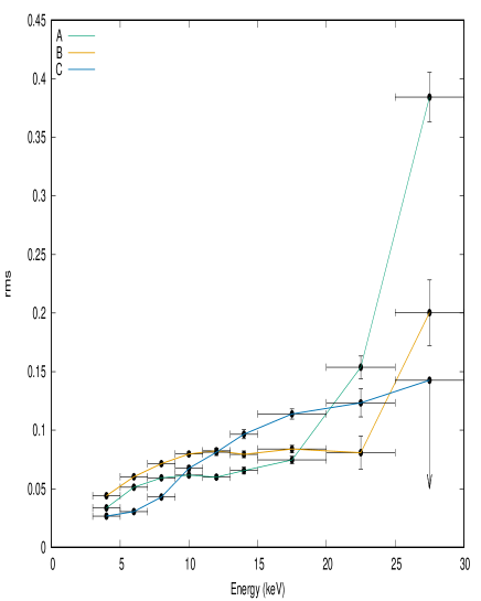
For obtaining the HID for dataset 1, lightcurves were generated in the energy bands viz. 3.0-18.0 keV, 7.5-10.5 keV and 10.5-18.0 keV energy range (Agrawal et al. 2018), where hardness ratio is that between the count rates in 7.5-10.5 keV and 10.5-18.0 keV energy bands and intensity is that in the 3.0-18.0 keV energy range (Fig. 2, For more details see Malu et al. (2021)). Based on the HID of both datasets, 4U 1705-44 is found to be in the banana state. The HID was divided into 3 parts for Dataset 1 - A, B and C sections in order to study the energy-rms relation, Power Density Spectra (PDS) and CCFs. Figure 3 shows that energy-rms plot for light curves of the three sections - A, B and C. Light curves where obtained in the 3-5 keV, 5-7 keV, 7-9 keV, 9-11 keV, 11-13 keV, 13-15 keV, 15-20 keV, 20-25 keV and 25-30 keV in order to determine the fractional rms variation in the light curve. The trend is found to be increasing in all the three cases, as often seen in these sources. Right panel of the figure gives the PDS of the three sections respectively in the 3-30 keV energy range using a lightcurve of 1/512 s binsize (described later in detail).

Refer to caption — Fig. 1 : Top: Lightcurve (dataset 1) of 4U 1705-44 obtained from LAXPC 10 binned with 32 s binsize in the 3-30 keV energy band. Bottom: Same for dataset 2.

4.1 Cross-Correlation Function study

Lightcurves in the 3-5 keV (soft) and 15-30 keV (hard) energy bands were extracted for performing CCF studies. The crosscor tool available in the XRONOS package was utilized for performing the cross correlation analysis (see Sriram et al. 2007, 2011, 2012, 2019, Lei et al. 2008, 2013 and Malu et al. 2020). The crosscor tool uses a FFT or a direct slow (option fast=no) algorithm to compute cross-correlation between two simultaneous light curves and gives an output of CC value as a function of time delay. We have used the slow direct mode and in this mode the CCF error bars are obtained by propagating the theoretical error bars of the cross correlations from individual intervals that are in turn obtained by propagating the newbin error bars through the cross correlation formula¹¹1https://heasarc.gsfc.nasa.gov/docs/xanadu/xronos/help/crosscor.html. These cross-correlations are then normalized by dividing them by the square root of the product of the number of good newbins of the two time series in each interval, to obtain the cross covariances.

A 10 s bin size was used during the CCF analysis and lags were obtained in ten different light curve segments of the order of hundred seconds (Fig. 4, 5). Gaussian function was fitted on the data points around the most significant peak in the CCF profile with a 90% confidence level (Fig. 6). A $\chi$ ² minimization method with the criterion of $\Delta$ $\chi$ ² = 2.7, was used in order to determine the CCF lag values and the corresponding errors (Table 2).

Asymmetric CCF profiles are difficult to judge and they clearly can not be approximated by a Gaussian profile. We have used the Gaussian profile fitting method only on those CCF profiles that are relatively symmetric and could be approximated to a Gaussian profile. For this we have set a criterion of $\chi$ ²/dof $<$ 2. Even so, the lags thus estimated should be cautiously taken. For further results we have only considered those lag values that were best constrained with lower error bars following our set criterion. Larger uncertainties in the CCF lag estimation would directly lead to larger disparities in the results further discussed. The $\chi$ ²/dof values would depend upon the number of points around the peak CC that are considered for the fit. Errors and lag values would depend upon this consideration eventually.

For dataset 1, amongst the observation during 12 orbits, three lightcurve segments exhibited lags. Figure 4a-c shows the lightcurve segments and the corresponding CCFs of each segment. Segments that showed delays had symmetric profiles and low error bars. Hence, all the three sections that showed lags were considered for further studies. While one light curve segment showed anti-correlated hard lags of 371 $\pm$ 7 s (CC = -0.53 $\pm$ 0.06), one segment showed an anti-correlated soft lag of 163 $\pm$ 9 s (CC = -0.47 $\pm$ 0.08) (see fig. 4a-c. Table 2). CCF in Fig. 4c. (top panel) peaks positively at 0 and negatively at $\sim$ 258 s (hard lag) both with similar CC values, hence in such a case specifying the exact nature and occurrence of the lag is rather tough.

By hard lag we are referring to the hard photons lagging the soft photons and the opposite scenario for the soft lags. Most of the remaining segments were positively correlated with no lag (CC $\sim$ 0.6-0.8) while few other segments were uncorrelated. All the lags noted lie in section A and B of the HID.

Table 2 : Obtained CCF lags in dataset 1 and 2 with their corresponding errors (90 % confidence limits) and the best fit

\chi

²/dof.

	Dataset 1
CCF lag $\pm$ error (s)	CC $\pm$ error	$\chi$ ²/dof	Corresponding Figures
371 $\pm$ 7	-0.53 $\pm$ 0.06	46.13/66	Fig. 4a (bottom panel)
-163 $\pm$ 9	-0.47 $\pm$ 0.08	22.24/29	Fig. 4b (bottom panel)
	Dataset 2
64 $\pm$ 6	0.53 $\pm$ 0.10	22.64/27	Fig. 5a (bottom panel)
-274 $\pm$ 21	-0.27 $\pm$ 0.09	52.05/77	Fig. 5b
-137 $\pm$ 14	-0.28 $\pm$ 0.05	146.3/109	Fig. 5c (top panel)
-533 $\pm$ 8	-0.50 $\pm$ 0.06	69.92/109	Fig. 5d (bottom panel)
573 $\pm$ 28	-0.31 $\pm$ 0.05	391.8/276	Fig. 5e
-450 $\pm$ 21	0.31 $\pm$ 0.05	140.9/197	Fig. 5f
238 $\pm$ 15	-0.31 $\pm$ 0.10	47.64/70	Fig. 5g (bottom panel)