Broken-FEEC discretizations and Hodge Laplace problems

Abstract

This article studies structure-preserving discretizations of Hilbert complexes with nonconforming (broken) spaces that rely on projection operators onto an underlying conforming subcomplex. This approach follows the conforming/nonconforming Galerkin (CONGA) method introduced in [15, 16, 17] to derive efficient structure-preserving finite element schemes for the time-dependent Maxwell and Maxwell-Vlasov systems by relaxing the curl-conforming constraint in finite element exterior calculus (FEEC) spaces. Here, it is extended to the discretization of full Hilbert complexes with possibly nontrivial harmonic fields, and the properties of the resulting CONGA Hodge Laplacian operator are investigated.

By using block-diagonal mass matrices which may be locally inverted, this framework possesses a canonical sequence of dual commuting projection operators which are local in standard finite element applications, and it naturally yields local discrete coderivative operators, in contrast to conforming FEEC discretizations. The resulting CONGA Hodge Laplacian operator is also local, and its kernel consists of the same discrete harmonic fields as the underlying conforming operator, provided that a symmetric stabilization term is added to handle the space nonconformities.

Under the assumption that the underlying conforming subcomplex admits a bounded cochain projection, and that the conforming projections are stable with moment-preserving properties, a priori convergence results are established for both the CONGA Hodge Laplace source and eigenvalue problems. Our theory is finally illustrated with a spectral element method, and numerical experiments are performed which corroborate our results. Applications to spline finite elements on multi-patch mapped domains are described in a related article [22], for which the present work provides a theoretical background.

1 Introduction

Over the last few decades, an important body of work has been devoted to the development of compatible finite element methods that preserve the structure of de Rham complexes involved in fluid and electromagnetic models. In addition to providing faithful approximations of the Hodge-Helmholtz decompositions at the discrete level, such discretizations indeed possess intrinsic stability and spectral correctness properties [9, 23, 1, 6, 12]. A notable step has been the unifying analysis of finite element exterior calculus (FEEC) [2, 3] developped in the general framework of Hilbert complexes with further applications in solid mechanics, and where the existence of bounded cochain projections, i.e. sequences of commuting projection operators with uniform stability properties, has been identified as a key ingredient for discrete stability and structure preservation.

More recently, structure-preserving discretizations have been extended to nonconforming (broken) finite element spaces associated to sequences of conforming subspaces via stable projection operators. The primary motivation for this was to improve the computational efficiency of numerical approximations to time-dependent Maxwell [15] and Maxwell-Vlasov equations [16, 17], where conforming FEEC schemes with high order elements, non-cartesian coordinates or non-scalar permittivities usually require a global inversion of the mass matrix, which in turn results in the discrete coderivatives being global operators. This difficulty is naturally resolved with broken spaces as the mass matrices become block diagonal. In contractible domains where the de Rham sequence is exact, the resulting conforming/nonconforming Galerkin (CONGA) method has been shown to have long time stability, be spectrally correct and preserve key physical invariants such as the Gauss laws, without requiring numerical stabilization mechanisms as commonly used in discontinuous Galerkin schemes.

In this article we extend these works in several directions. First, we consider the discretization of full Hilbert complexes with general Hodge cohomology, and we exhibit a canonical mechanism to build stable commuting projections for the dual (weak) discrete complex. This shows in particular that broken FEEC discretizations provide a ready-to-use framework for nonconforming Hamiltonian particle approximations to Maxwell-Vlasov equations, with either strong or weak particle-field coupling. We then study the associated CONGA Hodge Laplacian operator with a stabilization term for the space nonconformity. For arbitrary positive values of the stabilization parameter, we find that this operator has the same kernel as its conforming counterpart, namely discrete harmonic fields, and we establish several decompositions of the broken spaces that generalize the discrete Hodge-Helmholtz decompositions of conforming FEEC spaces. The associated source problem is next shown to be well-posed. Under the assumption that the conforming projection operators are uniformly stable with moment-preserving properties, we establish a priori error estimates that allow us to recover the main stability and convergence properties of conforming FEEC approximations. For stronger penalization regimes, our error estimates also show the spectral correctness of the CONGA Hodge Laplacian operator. Finally we describe an application to polynomial finite elements, where this framework naturally yields local discrete differential operators for both the primal (strong) and dual (weak) sequences, as well as local $L^{2}$-stable dual commuting projection operators.

We point out that for Cartesian meshes or low-order elements, there exist lumping methods based on approximate quadrature rules which allow one to derive local approximations of the inverse mass matrices, see e.g. [19, 20], as well as local dual differential operators [27, 26]. While the extension of these methods to high-order elements on unstructured or curvilinear cells is yet unclear, the CONGA method has no such limitations: the theory presented in this article naturally extends to curvilinear grids (see [22] for an application to spline finite elements on multi-patch mapped domains) as well as unstructured grids (following the same lines as in [16, 17]).

The outline is as follows. After recalling the main ingredients of conforming FEEC discretizations of closed Hilbert complexes in Section 2, we describe its extension on broken spaces with projection-based differential operators in Section 3, where the CONGA Hodge Laplacian operator is also presented. The source and eigenvalue problems are then studied in Section 4, where the a priori convergence results are established. We conclude with an application to polynomial finite elements in Section 5, and exhibit numerical results which confirm some of our theoretical findings.

2 Hilbert complexes and FEEC discretizations

Following [3] we consider a closed Hilbert complex $(W,d)=(W^{\ell},d^{\ell})_{\ell\in\mathbbm{N}}$ involving unbounded, closed operators $d^{\ell}:W^{\ell}\to W^{\ell+1}$ with dense domains $V^{\ell}$ and closed images $d^{\ell}V^{\ell}\subset\ker d^{\ell+1}$ implying in particular $d^{\ell+1}d^{\ell}=0$. Denoting by $\lVert\cdot\rVert$ the Hilbert norms of the $W$ spaces, and droping the $\ell$ indices when they are clear from the context, the domain spaces are equipped with the graph norm $\lVert v\rVert^{2}_{V}=\lVert v\rVert^{2}+\lVert dv\rVert^{2}$, which makes the domain complex

$$V^{\ell-1}~{}\xrightarrow{\hskip 2.0pt\displaystyle d^{\ell-1}\hskip 2.0pt}~{}V^{\ell}~{}\xrightarrow{\hskip 2.0pt\displaystyle d^{\ell}\hskip 2.0pt}~{}V^{\ell+1}$$ (2.1)

a bounded Hilbert complex. By identifying each $W^{\ell}$ space with its dual, we obtain a dual complex (denoted with lower indices to reflect its reverse order)

$$V^{*}_{\ell-1}~{}\xleftarrow{\hskip 2.0pt\displaystyle d^{*}_{\ell}\hskip 2.0pt}~{}V^{*}_{\ell}~{}\xleftarrow{\hskip 2.0pt\displaystyle d^{*}_{\ell+1}\hskip 2.0pt}~{}V^{*}_{\ell+1}$$ (2.2)

where the operators $d^{*}=d^{*}_{\ell+1}:W^{\ell+1}\to W^{\ell}$ are the unbounded adjoints of the $d^{\ell}$’s. We remind that they are characterized by the relations

$$\langle d^{*}_{\ell+1}w,v\rangle=\langle w,d^{\ell}v\rangle\qquad\forall w\in V^{*}_{\ell+1},~{}v\in V^{\ell}$$ (2.3)

on their domains $V^{*}_{\ell+1}:=\{w\in W^{\ell+1}:\lvert\langle w,d^{\ell}v\rangle\rvert\leq C_{w}\lVert v\rVert,\forall v\in V^{\ell}\}$, see e.g. [10], where $\langle\cdot,\cdot\rangle$ denotes the Hilbert product in the $W$ spaces, so that (2.3) essentially amounts to an integration by parts with no boundary terms. As in [3] we denote the ranges and kernels of the primal operators by

$$\mathfrak{B}^{\ell}:=\operatorname{Im}(d^{\ell-1})=dV^{\ell-1}\subset V^{\ell}\qquad\text{ and }\qquad\mathfrak{Z}^{\ell}:=\ker(d^{\ell})\subset V^{\ell}$$

and similarly for the dual operators,

$$\mathfrak{B}^{*}_{\ell}:=\operatorname{Im}(d^{*}_{\ell+1})=d^{*}V^{*}_{\ell+1}\subset V^{*}_{\ell}\qquad\text{ and }\qquad\mathfrak{Z}^{*}_{\ell}:=\ker(d^{*}_{\ell})\subset V^{*}_{\ell}.$$

Since the operators are closed and densely defined with closed ranges we have

$$\mathfrak{B}^{\ell}=(\mathfrak{Z}^{*}_{\ell})^{{\perp_{W}}}\qquad\text{ and }\qquad\mathfrak{B}^{*}_{\ell}=(\mathfrak{Z}^{\ell})^{{\perp_{W}}}$$

see [10], where ${\perp_{W}}$ denotes the orthogonal complement in the proper $W$ space.

2.1 Hodge Laplacian operator

The Hodge Laplacian operator

$$L:=dd^{*}+d^{*}d$$ (2.4)

is a self-adjoint unbounded operator $L^{\ell}=d^{\ell-1}d^{*}_{\ell}+d^{*}_{\ell+1}d^{\ell}:W^{\ell}\to W^{\ell}$ with domain

$$D(L^{\ell})=\{u\in V^{\ell}\cap V^{*}_{\ell}:d^{\ell}u\in V^{*}_{\ell+1},d^{*}_{\ell}u\in V^{\ell-1}\}.$$ (2.5)

Its kernel and image spaces read

$$\ker L^{\ell}=(\mathfrak{B}^{\ell})^{\perp_{W}}\cap\mathfrak{Z}^{\ell}=:\mathfrak{H}^{\ell}\qquad\text{ and }\qquad\operatorname{Im}L^{\ell}=(\mathfrak{H}^{\ell})^{{\perp_{W}}}$$

where $\mathfrak{H}^{\ell}$ is the space of harmonic fields. If the latter is not trivial, the source problem

$$L^{\ell}u=f$$ (2.6)

is ill-posed, but it can be corrected by projecting a general source $f\in W^{\ell}$ and constraining the solution. The resulting problem consists of finding $u\in(\mathfrak{H}^{\ell})^{{\perp_{W}}}$ such that $L^{\ell}u=f-Q_{\mathfrak{H}}f$, where $Q_{\mathfrak{H}}$ is the $W$-orthogonal projection on $\mathfrak{H}^{\ell}$. It may be recast in a mixed form:

$$\text{ Find }\quad(\sigma,u,p)\in X:=V^{\ell-1}\times V^{\ell}\times\mathfrak{H}^{\ell},\quad\text{ such that }$$ (2.7)

$$\left\{\begin{aligned} \langle\sigma,\tau\rangle-\langle d\tau,u\rangle&=0\qquad&&\forall\tau\in V^{\ell-1}\\ \langle d\sigma,v\rangle+\langle du,dv\rangle+\langle v,p\rangle&=\langle f,v\rangle\qquad&&\forall v\in V^{\ell}\\ \langle u,q\rangle&=0\qquad&&\forall q\in\mathfrak{H}^{\ell}.\end{aligned}\right.$$

An equivalent formulation is to find $(\sigma,u,p)\in X$ such that

$$b(\sigma,u,p;\tau,v,q)=\langle f,v\rangle\qquad\forall(\tau,v,q)\in X$$ (2.8)

with the bilinear form

$$b(\sigma,u,p;\tau,v,q):=\langle\sigma,\tau\rangle-\langle d\tau,u\rangle+\langle d\sigma,v\rangle+\langle du,dv\rangle+\langle v,p\rangle-\langle u,q\rangle.$$ (2.9)

The well-posedness of this problem essentially relies on the closed complex property which leads to a generalized Poincaré inequality of the form

$$\lVert v\rVert_{V}\leq c_{P}\lVert dv\rVert,\qquad v\in V^{\ell}\cap(\mathfrak{Z}^{\ell})^{{\perp_{W}}}$$ (2.10)

using Banach’s bounded inverse theorem. It is indeed shown in [3, Th. 3.2] that for all $(\sigma,u,p)\in X$, there exists $(\tau,v,q)\in X$ for which

$$b(\sigma,u,p;\tau,v,q)\geq\gamma(\lVert\sigma\rVert_{V}+\lVert u\rVert_{V}+\lVert p\rVert)(\lVert\tau\rVert_{V}+\lVert v\rVert_{V}+\lVert q\rVert)$$ (2.11)

holds with a constant $\gamma>0$ depending only on the Poincaré constant $c_{P}$. Noting that $b(\sigma,u,p;\tau,v,q)=b(\tau,-v,q;\sigma,-u,p)$, this leads to the inf-sup condition

$$\inf_{y\in X}\sup_{x\in X}\frac{b(x,y)}{\lVert x\rVert_{X}\lVert y\rVert_{X}}\geq\gamma>0$$ (2.12)

where $X=V^{\ell-1}\times V^{\ell}\times\mathfrak{H}^{\ell}$ is equipped with $\lVert(\tau,v,q)\rVert_{X}=\lVert\tau\rVert_{V}+\lVert v\rVert_{V}+\lVert q\rVert$. Classically, the inf-sup condition (2.12) implies that the operator $B:X\to X^{\prime}$ defined by $\langle Bx,y\rangle_{X^{\prime}\times X}=b(x,y)$ is surjective [7], and it is clearly injective by (2.11). Hence (2.8) admits a unique solution, which satisfies

$$\lVert\sigma\rVert_{V}+\lVert u\rVert_{V}+\lVert p\rVert\leq\gamma^{-1}\lVert f\rVert.$$

2.2 Conforming FEEC discretization

The usual discretization is provided by a finite dimensional subcomplex of the form

$$V^{\ell-1,c}_{h}~{}\xrightarrow{\hskip 2.0pt\displaystyle d^{\ell-1,c}_{h}\hskip 2.0pt}~{}V^{\ell,c}_{h}~{}\xrightarrow{\hskip 2.0pt\displaystyle d^{\ell,c}_{h}\hskip 2.0pt}~{}V^{\ell+1,c}_{h}$$ (2.13)

where the discrete differential operators are the restrictions of the continuous ones,

$$d^{\ell,c}_{h}=d^{\ell}:V^{\ell,c}_{h}\to V^{\ell+1,c}_{h}~{}.$$ (2.14)

Here the $c$ superscript indicates that these discrete spaces are conforming in the sense that $V^{\ell,c}_{h}\subset V^{\ell}$. This notation somehow deviates from the usual one ($V^{\ell}_{h}$) which we will use for the broken spaces in Section 3, since they are the focus of this article. A key result [2, 3] is that the stability of the conforming discretization relies on the existence of a bounded cochain projection $\pi_{h}$, i.e. projection operators $\pi^{\ell}_{h}:V^{\ell}\to V^{\ell,c}_{h}$ that satisfy the commuting diagram property

$$d^{\ell}\pi^{\ell}_{h}=\pi^{\ell+1}_{h}d^{\ell}\qquad\text{ on }~{}V^{\ell}$$ (2.15)

such that $\lVert\pi_{h}v\rVert_{V}\leq\lVert\pi_{h}\rVert_{V}\lVert v\rVert_{V}$ for all $v\in V^{\ell}$, with an operator norm $\lVert\pi_{h}\rVert_{V}$ bounded independent of $h$. Throughout the article the notation $\lVert\cdot\rVert_{V}$ will be used for both the $V$ norm and the operator norm in $V$.

Remark 2.1 (discretization parameter $h$).

Here and below, the subscript $h$ loosely represents a discretization parameter that can be varied to improve the resolution of the discrete spaces. Typically this parameter corresponds to a mesh size, but in most places (and unless specified otherwise) it may represent arbitrary discretization parameters. What matters in the analysis is that several properties will hold with constants independent of it. Classically these constants will be denoted with the generic letter $C$, whose value may change at each occurrence.

The dual discrete complex involves the same discrete spaces: it reads

$$V^{\ell-1,c}_{h}~{}\xleftarrow{\hskip 2.0pt\displaystyle d^{*,c}_{\ell,h}\hskip 2.0pt}~{}V^{\ell,c}_{h}~{}\xleftarrow{\hskip 2.0pt\displaystyle d^{*,c}_{\ell+1,h}\hskip 2.0pt}~{}V^{\ell+1,c}_{h}$$ (2.16)

where $d^{*,c}_{\ell+1,h}:V^{\ell+1,c}_{h}\to V^{\ell,c}_{h}$ is the adjoint of $d^{\ell,c}_{h}$, i.e.

$$\langle d^{*,c}_{\ell+1,h}q,v\rangle=\langle q,d^{\ell}v\rangle,\qquad\forall v\in V^{\ell,c}_{h}.$$ (2.17)

In similarity to the continuous case (and omitting again the $\ell$ indices when they are clear from the context), we denote the discrete kernels and ranges by

$$\mathfrak{B}^{\ell,c}_{h}:=\operatorname{Im}d^{\ell-1,c}_{h}=d^{c}_{h}V^{\ell-1,c}_{h}\qquad\text{ and }\qquad\mathfrak{Z}^{\ell,c}_{h}:=\ker d^{\ell,c}_{h}$$ (2.18)

and similarly for the discrete adjoint operators,

$$\mathfrak{B}^{*,c}_{\ell,h}:=\operatorname{Im}d^{*,c}_{\ell+1,h}=d^{*,c}_{h}V^{\ell+1,c}_{h}\qquad\text{ and }\qquad\mathfrak{Z}^{*,c}_{\ell,h}:=\ker d^{*,c}_{\ell,h}$$ (2.19)

where we notice that these four spaces are all subspaces of $V^{\ell,c}_{h}$. As the discrete operators are all closed and bounded with closed range, we also have

$$\mathfrak{B}^{\ell,c}_{h}=V^{\ell,c}_{h}\cap(\mathfrak{Z}^{*,c}_{\ell,h})^{\perp_{W}}=:\mathfrak{Z}^{*,c\perp}_{\ell,h}$$ (2.20)

and similarly

$$\mathfrak{B}^{*,c}_{\ell,h}=V^{\ell,c}_{h}\cap(\mathfrak{Z}^{\ell,c}_{h})^{\perp_{W}}=:\mathfrak{Z}^{\ell,c\perp}_{h}~{}.$$ (2.21)

It follows from the basic sequence property $d^{\ell,c}_{h}d^{\ell+1,c}_{h}=0$ that $\mathfrak{B}^{\ell,c}_{h}\subset\mathfrak{Z}^{\ell,c}_{h}$, in particular $\mathfrak{B}^{\ell,c}_{h}$ and $\mathfrak{B}^{*,c}_{\ell,h}=\mathfrak{Z}^{\ell,c\perp}_{h}$ are orthogonal. Denoting the complement space as

$$\mathfrak{H}^{\ell,c}_{h}:=(\mathfrak{B}^{\ell,c}_{h})^{\perp_{W}}\cap\mathfrak{Z}^{\ell,c}_{h}\subset V^{\ell,c}_{h},$$ (2.22)

yields a discrete Hodge-Helmholtz decomposition for the conforming space,

$$V^{\ell,c}_{h}=\mathfrak{B}^{\ell,c}_{h}\overset{\perp}{\oplus}\mathfrak{H}^{\ell,c}_{h}\overset{\perp}{\oplus}\mathfrak{B}^{*,c}_{\ell,h}.$$ (2.23)

2.3 Discrete Hodge Laplacian operator

The conforming discrete Hodge Laplacian operator is

$$L^{c}_{h}:=d^{c}_{h}d^{*,c}_{h}+d^{*,c}_{h}d^{c}_{h}$$ (2.24)

specifically, $L^{c}_{h}=L^{\ell,c}_{h}=d^{\ell-1,c}_{h}d^{*,c}_{\ell,h}+d^{*,c}_{\ell+1,h}d^{\ell,c}_{h}:V^{\ell,c}_{h}\to V^{\ell,c}_{h}$. Its kernel consists of the discrete harmonic fields, namely the $v\in V^{\ell}_{h}$ for which both $d^{*,c}_{\ell,h}=0$ and $d^{\ell,c}_{h}v=0$. From (2.18)–(2.23) one infers that

$$\ker L^{\ell,c}_{h}=\mathfrak{Z}^{*,c}_{\ell,h}\cap\mathfrak{Z}^{\ell,c}_{h}=\mathfrak{H}^{\ell,c}_{h}.$$ (2.25)

Using the fact that $d^{c}_{h}=d$ on the discrete conforming spaces, the corresponding source problem in mixed form reads:

$$\text{ Find }\quad(\sigma^{c}_{h},u^{c}_{h},p^{c}_{h})\in X^{c}_{h}:=V^{\ell-1,c}_{h}\times V^{\ell,c}_{h}\times\mathfrak{H}^{\ell,c}_{h}\quad\text{ such that }$$ (2.26)

$$\left\{\begin{aligned} \langle\sigma^{c}_{h},\tau\rangle-\langle d\tau,u^{c}_{h}\rangle&=0\qquad&&\forall\tau\in V^{\ell-1,c}_{h}\\ \langle d\sigma^{c}_{h},v\rangle+\langle du^{c}_{h},dv\rangle+\langle v,p^{c}_{h}\rangle&=\langle f,v\rangle\qquad&&\forall v\in V^{\ell,c}_{h}\\ \langle u^{c}_{h},q\rangle&=0\qquad&&\forall q\in\mathfrak{H}^{\ell,c}_{h}~{}.\end{aligned}\right.$$

The stability of Problem (2.26) then relies on a discrete Poincaré inequality

$$\lVert v\rVert_{V}\leq c_{P,h}\lVert dv\rVert,\qquad v\in\mathfrak{Z}^{\ell,c\perp}_{h}$$ (2.27)

see (2.21), which itself follows from the existence of a bounded cochain projection. Indeed the following results holds, see [3, Th. 3.6 and 3.8], which leads to the well-posedness of Problem (2.26) in similarity to the continuous case.

Theorem 2.2.

If the conforming discrete complex $(V^{c}_{h},d)$ admits a $V$-bounded cochain projection (2.15), then the discrete Poincaré inequality (2.27) holds with a constant $c_{P,h}=c_{P}\lVert\pi_{h}\rVert_{V}$ where $c_{P}$ is from (2.10). Moreover, for any $(\sigma,u,p)\in X^{c}_{h}=V^{\ell-1,c}_{h}\times V^{\ell,c}_{h}\times\mathfrak{H}^{\ell,c}_{h}$, there exists $(\tau,v,q)\in X^{c}_{h}$ such that

$$b(\sigma,u,p;\tau,v,q)\geq\gamma(\lVert\sigma\rVert_{V}+\lVert u\rVert_{V}+\lVert p\rVert)(\lVert\tau\rVert_{V}+\lVert v\rVert_{V}+\lVert q\rVert)$$

holds for some $\gamma>0$ depending only on the discrete Poincaré constant $c_{P,h}$. In particular, Problem (2.26) is well-posed.

We finally remind that Problem (2.26) is equivalent to finding $u^{c}_{h}\in V^{\ell,c}_{h}\cap(\mathfrak{H}^{\ell,c}_{h})^{\perp_{W}}$ such that $L^{\ell,c}_{h}u^{c}_{h}=Q_{V^{c}_{h}}f-Q_{\mathfrak{H}^{c}_{h}}f$, with $\sigma^{c}_{h}=d^{*,c}_{\ell,h}u^{c}_{h}$ and $p^{c}_{h}=Q_{\mathfrak{H}^{c}_{h}}f$. (Throughout the article $Q_{U}$ denotes the $W$-orthogonal projection onto a closed subspace $U$.) Indeed, each component of the solution in the discrete decomposition

$$u^{c}_{h}=u^{c}_{\mathfrak{B}}+u^{c}_{\mathfrak{H}}+u^{c}_{\mathfrak{B}^{*}}~{}\in~{}\mathfrak{B}^{\ell,c}_{h}\overset{\perp}{\oplus}\mathfrak{H}^{\ell,c}_{h}\overset{\perp}{\oplus}\mathfrak{B}^{*,c}_{\ell,h}$$ (2.28)

may be characterized by taking test functions in the suitable subspaces: we have

$$\left\{\begin{aligned} \langle\sigma^{c}_{h},\tau\rangle-\langle d\tau,u^{c}_{\mathfrak{B}}\rangle&=0\qquad&&\forall\,\tau\in V^{\ell-1,c}_{h}\\ \langle d\sigma^{c}_{h},v\rangle&=\langle f,v\rangle\qquad&&\forall\,v\in\mathfrak{B}^{\ell,c}_{h}~{},\end{aligned}\right.$$ (2.29)

the harmonic component is $u^{c}_{\mathfrak{H}}=0$, and

$$\langle du^{c}_{\mathfrak{B}^{*}},dv\rangle=\langle f,v\rangle\qquad\forall\,v\in\mathfrak{B}^{*,c}_{\ell,h}~{}.$$ (2.30)

Taking $v\in\mathfrak{H}^{\ell,c}_{h}$ finally yields $p^{c}_{h}=Q_{\mathfrak{H}^{c}_{h}}f$.

3 Broken FEEC discretization

We now study a discretization of the Hilbert complex (2.1) where the conformity requirement is relaxed. Specifically, we assume in this section that we are given a conforming discretization (2.13) and we consider at each level $\ell$ a discrete space $V^{\ell}_{h}\subset W^{\ell}$ that contains the conforming one,

$$V^{\ell,c}_{h}\subset V^{\ell}_{h}$$ (3.1)

but is not necessarily a subspace of $V^{\ell}$. The typical situation that we have in mind is the one where the conforming spaces have some finite element structure of the form $V^{\ell,c}_{h}=\big{(}\mathbbm{V}^{\ell}(\Omega_{1})\times\dots\times\mathbbm{V}^{\ell}(\Omega_{K})\big{)}\cap V^{\ell}$ on a partition of the domain $\Omega$ into subdomains $\Omega_{k}$, $k=1,\dots K$, and where the conformity $V^{\ell,c}_{h}\subset V^{\ell}$ amounts to continuity constraints on the subdomain interfaces, see e.g. [7, 22] and Section 5. Working with the broken spaces $V^{\ell}_{h}=\mathbbm{V}^{\ell}(\Omega_{1})\times\dots\times\mathbbm{V}^{\ell}(\Omega_{K})$ allows one to lift these constraints, yielding more locality for the discrete operators and more flexibility in the numerical modelling.

Since our analysis is based on a stable conforming discretization, we make this assumption explicit.

Assumption 3.1.

The conforming sequence $V^{c}_{h}$ admits a uniformly $V$-bounded cochain projection (2.15). According to Theorem 2.2 this implies that the discrete Poincaré inequality (2.27) holds with a constant

$$0<c_{P,h}\leq\bar{c}_{P}$$ (3.2)

where $\bar{c}_{P}$ is independent of the discretization parameter $h$.

3.1 Projection-based differential operators

A discrete Hilbert complex involving the broken spaces can be obtained by considering projection operators onto the conforming subspaces,

$$P^{\ell}_{h}:V^{\ell}_{h}\to V^{\ell,c}_{h}\subset V^{\ell}_{h}$$ (3.3)

and by defining discrete differential operators on the broken spaces as

$$d^{\ell}_{h}:=d^{\ell}P^{\ell}_{h}~{}.$$ (3.4)

These operators map $V^{\ell}_{h}$ to $V^{\ell+1,c}_{h}\subset V^{\ell+1}_{h}$, and by the projection property they satisfy $d^{\ell}_{h}d^{\ell-1}_{h}=d^{\ell}d^{\ell-1}P^{\ell-1}_{h}=0$, hence we indeed obtain a discrete Hilbert complex,

$$V^{\ell-1}_{h}\xrightarrow{\mbox{$~{}d^{\ell-1}_{h}~{}$}}V^{\ell}_{h}\xrightarrow{\mbox{$~{}d^{\ell}_{h}~{}$}}V^{\ell+1}_{h}.$$ (3.5)

This construction may be summarized by the following diagram where the horizontal sequences are Hilbert complexes and the vertical arrows denote projection operators.

We note that this diagram commutes, since the strong differential operators map onto the conforming spaces. For the subsequent analysis we equip the broken spaces with Hilbert norms

$$\lVert v\rVert_{V_{h}}^{2}=\lVert v\rVert^{2}+\lVert dP_{h}v\rVert^{2},\qquad v\in V^{\ell}_{h},$$ (3.6)

and assume that the operators $P_{h}$ are bounded uniformly in $W$, namely that

$$\lVert P_{h}v\rVert\leq C\lVert v\rVert\quad\forall v\in V^{\ell}_{h}$$ (3.7)

holds with a constant independent of $h$, see Remark 2.1. Again, for conciseness we sometimes drop the level indices $\ell$ when they are clear from the context.

As in the conforming case, a dual discrete sequence is built on the same spaces

$$V^{\ell-1}_{h}~{}\xleftarrow{\hskip 2.0pt\displaystyle d^{*}_{\ell,h}\hskip 2.0pt}~{}V^{\ell}_{h}~{}\xleftarrow{\hskip 2.0pt\displaystyle d^{*}_{\ell+1,h}\hskip 2.0pt}~{}V^{\ell+1}_{h}$$ (3.8)

by introducing the discrete adjoint operators $d^{*}_{\ell+1,h}:=(d^{\ell}_{h})^{*}:V^{\ell+1}_{h}\to V^{\ell}_{h}$ defined as

$$\langle d^{*}_{\ell+1,h}q,v\rangle=\langle q,d^{\ell}P^{\ell}_{h}v\rangle,\qquad\forall v\in V^{\ell}_{h}.$$ (3.9)

The CONGA (broken FEEC) Hodge Laplacian operator is then defined as

$$L_{h}:=d_{h}d^{*}_{h}+d^{*}_{h}d_{h}$$ (3.10)

and a stabilized version is

$$L_{h,\alpha}:=L_{h}+\alpha(I-P_{h}^{*})(I-P_{h})$$ (3.11)

namely, $L^{\ell}_{h,\alpha}=d^{\ell-1}_{h}d^{*}_{\ell,h}+\alpha(I-(P^{\ell}_{h})^{*})(I-P^{\ell}_{h})+d^{*}_{\ell+1,h}d^{\ell}_{h}:V^{\ell}_{h}\to V^{\ell}_{h}$. Here the stabilization term involves the adjoint $P_{h}^{*}:=(P^{\ell}_{h})^{*}:V^{\ell}_{h}\to V^{\ell}_{h}$ of the discrete conforming projection, and a parameter $\alpha\geq 0$. In the regimes where $\alpha\to\infty$ as the discretization parameter $h$ is refined, this term may be seen as a penalization of the nonconformities. However, an arbitrary positive stabilization is sufficient to recover the conforming harmonic fields (2.22) as the kernel of the broken operator.

Theorem 3.2.

The CONGA Hodge Laplacian operator is a symmetric positive semi-definite operator in $V^{\ell}_{h}$. For a stabilization parameter $\alpha>0$, its kernel coincides with that of the conforming operator (2.25), i.e.

$$\ker L^{\ell}_{h,\alpha}=\mathfrak{H}^{\ell,c}_{h}$$ (3.12)

and its image is

$$\operatorname{Im}L^{\ell}_{h,\alpha}=\big{(}\mathfrak{H}^{\ell,c}_{h}\big{)}^{\perp_{h}}$$ (3.13)

where the ${\perp_{h}}$ exponent on a discrete space denotes the $W$-orthogonal complement in the natural broken space $V^{\ell}_{h}$.

The proof of this result relies on some decompositions of the nonconforming space $V^{\ell}_{h}$, which we will present in Section 3.3. Before doing so, we describe projections operators that commute with the dual differentials.

3.2 Commuting diagrams for strong and weak broken FEEC complexes

Before turning to the analysis of the Hodge Laplacian operator (3.10), we formalize and extend an observation previously made in [15], where it was shown that the adjoint of the conforming projection composed with the (local) $L^{2}$ projection onto the broken $H(\operatorname{curl})$ space commutes with the weak CONGA curl operator. In the full broken FEEC setting considered here this principle is generalized to the construction of a canonical sequence of stable projections that commute with the dual differential operators. These dual projections are defined as

$$\tilde{\pi}^{\ell}_{h}:=(P^{\ell}_{h})^{*}Q_{V^{\ell}_{h}}:W^{\ell}\to V^{\ell}_{h}$$ (3.14)

where we remind that $Q_{V^{\ell}_{h}}$ is the $W$-orthogonal projection onto $V^{\ell}_{h}$. Namely they are characterized by the relations

$$\langle\tilde{\pi}^{\ell}_{h}w,v\rangle=\langle w,P^{\ell}_{h}v\rangle,\quad\forall w\in W^{\ell},~{}v\in V^{\ell}_{h}.$$ (3.15)

Together with the stable commuting projection operators $\pi^{\ell}_{h}$ available for the conforming spaces $V^{\ell,c}_{h}\subset V^{\ell}_{h}$, this leads to a commuting diagram for both the primal (strong) and dual (weak) complexes.

Theorem 3.3.

The operators $\tilde{\pi}^{\ell}_{h}$ are uniformly $W$-stable projections onto the spaces

$$\operatorname{Im}\tilde{\pi}^{\ell}_{h}=(P^{\ell}_{h})^{*}V^{\ell}_{h}=\{v\in V^{\ell}_{h}:\langle v,(I-P^{\ell}_{h})w\rangle=0,~{}\forall w\in V^{\ell}_{h}\}~{}.$$ (3.16)

Moreover they commute with the dual differential operators:

$$d^{*}_{\ell,h}\tilde{\pi}^{\ell}_{h}=\tilde{\pi}^{\ell-1}_{h}d^{*}_{\ell}\qquad\text{ on }~{}V^{*}_{\ell}~{}.$$ (3.17)

In particular, under Assumption 3.1 we find that both the primal (top) and dual (bottom) diagram below commute.

Remark 3.4.

The projections $\tilde{\pi}^{\ell}_{h}$ are the broken-FEEC analogue of the $W$-orthogonal projection operators which commute with the dual differential operators in the conforming FEEC model. A key point is that here the broken nature of the spaces $V^{\ell}_{h}$ naturally leads to dual projection operators that are local when applied to standard finite elements spaces (see for instance Theorem 5.3 below), in contrast to what happens in the conforming case.

Proof. .

The $W$ stability is easily derived from that of $P^{\ell}_{h}$, indeed (3.7) allows us to write $\langle\tilde{\pi}^{\ell}_{h}w,v\rangle\leq\lVert w\rVert\lVert P^{\ell}_{h}v\rVert\leq C\lVert w\rVert\lVert v\rVert$, hence $\lVert\tilde{\pi}^{\ell}_{h}w\rVert\leq C\lVert w\rVert$ with the same constant as in (3.7). The projection property is also straightforward: given that $P^{\ell}_{h}$ is itself a projection, we see that $(\tilde{\pi}^{\ell}_{h})^{2}w\in V^{\ell}_{h}$ is characterized by

$$\langle(\tilde{\pi}^{\ell}_{h})^{2}w,v\rangle=\langle\tilde{\pi}^{\ell}_{h}w,P^{\ell}_{h}v\rangle=\langle w,(P^{\ell}_{h})^{2}v\rangle=\langle w,P^{\ell}_{h}v\rangle\quad\forall~{}v\in V^{\ell}_{h}$$

hence $(\tilde{\pi}^{\ell}_{h})^{2}w=\tilde{\pi}^{\ell}_{h}w$, and (3.16) follows from the fact that $\operatorname{Im}\tilde{\pi}^{\ell}_{h}=\operatorname{Im}(P^{\ell}_{h})^{*}=(\ker P^{\ell}_{h})^{{\perp_{h}}}$ (the symbol ${\perp_{h}}$ was introduced in Theorem 3.2) and $\ker P^{\ell}_{h}=\operatorname{Im}(I-P^{\ell}_{h})$. Finally the commuting property is a consequence of the weak definition of the dual differential operators: indeed for $v\in V^{*}_{\ell}$ and $\tau\in V^{\ell-1}_{h}$ it holds

$$\langle d^{*}_{\ell,h}\tilde{\pi}^{\ell}_{h}v,\tau\rangle=\langle\tilde{\pi}^{\ell}_{h}v,d^{\ell-1}_{h}\tau\rangle=\langle v,P^{\ell}_{h}d^{\ell-1}_{h}\tau\rangle=\langle v,d^{\ell-1}_{h}\tau\rangle\\ =\langle v,d^{\ell-1}P^{\ell-1}_{h}\tau\rangle=\langle d^{*}_{\ell}v,P^{\ell-1}_{h}\tau\rangle=\langle\tilde{\pi}^{\ell-1}_{h}d^{*}_{\ell}v,\tau\rangle$$

where the third equality uses the fact that $d^{\ell-1}_{h}$ maps into the conforming space $V^{\ell,c}_{h}$ where $P^{\ell}_{h}$ is the identity, and the fifth one uses the adjoint property (2.3) and the fact that $P^{\ell-1}_{h}\tau$ is in $V^{\ell-1,c}_{h}$, hence in $V^{\ell-1}$. ∎

An important by-product of our analysis is that broken-FEEC Maxwell solvers may be used to derive structure-preserving particle schemes, following the GEMPIC approach [24, 14]. Indeed the latter applies to general commuting de Rham diagrams, with no assumption of conformity.

Corollary 3.5.

By applying the variational discretization method from [14] to either the primal broken-FEEC sequence (3.5) or the dual one (3.8), and its associated primal or dual commuting projection operators, one obtains a Hamiltonian particle discretization of the Vlasov-Maxwell system with broken spaces for the field solver.

3.3 Broken Hodge-Helmholtz decompositions

As with the conforming operators, we define

$$\left\{\begin{aligned} &\mathfrak{B}^{\ell}_{h}:=\operatorname{Im}d^{\ell-1}_{h}\\ &\mathfrak{B}^{*}_{\ell,h}:=\operatorname{Im}d^{*}_{\ell+1,h}\end{aligned}\right.\quad\text{ and }\qquad\left\{\begin{aligned} &\mathfrak{Z}^{\ell}_{h}:=\ker d^{\ell}_{h}\\ &\mathfrak{Z}^{*}_{\ell,h}:=\ker d^{*}_{\ell,h}~{}.\end{aligned}\right.$$ (3.18)

These spaces may be related with the conforming ones in several ways. First, using (3.4) and the fact that $P^{\ell}_{h}$ is a projection onto the conforming space $V^{\ell,c}_{h}$, we observe that

$$\mathfrak{B}^{\ell}_{h}=d^{\ell-1}P^{\ell-1}_{h}V^{\ell-1}_{h}=d^{\ell-1}V^{\ell-1,c}_{h}=\mathfrak{B}^{\ell,c}_{h}$$ (3.19)

see (2.18). Next by using the analysis in [13] and (2.22) we obtain

$$\mathfrak{Z}^{\ell}_{h}=\mathfrak{Z}^{\ell,c}_{h}\oplus(I-P_{h}^{\ell})V^{\ell}_{h}=\mathfrak{B}^{\ell,c}_{h}\oplus\mathfrak{H}^{\ell,c}_{h}\oplus(I-P_{h})V^{\ell}_{h}$$ (3.20)

which also yields

$$\mathfrak{Z}^{\ell}_{h}\cap V^{\ell,c}_{h}=\mathfrak{Z}^{\ell,c}_{h}~{}.$$ (3.21)

Using the ${\perp_{h}}$ exponent to denote $W$-orthogonal complements in the natural $V^{\ell}_{h}$ space, as introduced in Theorem 3.2, we then write analogs to (2.21) and (2.20), namely

$$\mathfrak{B}^{\ell}_{h}=(\mathfrak{Z}^{*}_{\ell,h})^{\perp_{h}}=:\mathfrak{Z}^{*\perp}_{\ell,h}\qquad\text{ and }\qquad\mathfrak{B}^{*}_{\ell,h}=(\mathfrak{Z}^{\ell}_{h})^{\perp_{h}}=:\mathfrak{Z}^{\ell,\perp}_{h}$$ (3.22)

and similarly we observe that

$$(I-P_{h}^{*})V^{\ell}_{h}=\operatorname{Im}(I-P_{h}^{\ell})^{*}=(\ker(I-P_{h}^{\ell}))^{\perp_{h}}=(V^{\ell,c}_{h})^{\perp_{h}}~{}.$$ (3.23)

These relations allow us to study the kernel of the stabilized CONGA Hodge Laplacian operator.

Proof of Theorem 3.2. .

The first statement is obvious, since $L^{\ell}_{h,\alpha}$ (and $L^{\ell}_{h}$) is a sum of symmetric positive semi-definite operators. To show (3.12), we test $L^{\ell}_{h,\alpha}u=0$ against $u$: this yields

$$0=\langle L^{\ell}_{h,\alpha}u,u\rangle=\lVert d^{*}_{\ell,h}u\rVert^{2}+\alpha\lVert(I-P_{h})u\rVert^{2}+\lVert d^{\ell}_{h}u\rVert^{2}.$$

For $\alpha>0$ we thus have

$$\ker L^{\ell}_{h,\alpha}=\ker d^{*}_{\ell,h}\cap\ker(I-P_{h})\cap\ker d^{\ell}_{h}=\mathfrak{Z}^{*}_{\ell,h}\cap V^{\ell,c}_{h}\cap\mathfrak{Z}^{\ell}_{h}=\mathfrak{Z}^{*}_{\ell,h}\cap\mathfrak{Z}^{\ell,c}_{h}$$

where the last equality is (3.21). Using next (3.22) and (3.19) gives $\mathfrak{Z}^{*}_{\ell,h}=(\mathfrak{B}^{\ell,c}_{h})^{\perp_{h}}$, hence

$$\ker L^{\ell}_{h,\alpha}=(\mathfrak{B}^{\ell,c}_{h})^{\perp_{h}}\cap\mathfrak{Z}^{\ell,c}_{h}=(\mathfrak{B}^{\ell,c}_{h})^{\perp_{W}}\cap\mathfrak{Z}^{\ell,c}_{h}=\mathfrak{H}^{\ell,c}_{h}$$

according to the definition of the discrete harmonic forms (2.22). Finally (3.13) follows from the usual property $\operatorname{Im}A=(\ker A)^{\perp_{h}}$ for a symmetric operator $A:V_{h}\to V_{h}$. ∎

We conclude this section by establishing some generalized Hodge-Helmholtz decompositions for the broken spaces.

Lemma 3.6.

The broken space $V^{\ell}_{h}$ admits one orthogonal decomposition:

$$V^{\ell}_{h}=\mathfrak{B}^{\ell,c}_{h}\overset{\perp}{\oplus}\mathfrak{H}^{\ell,c}_{h}\overset{\perp}{\oplus}\mathfrak{B}^{*,c}_{\ell,h}\overset{\perp}{\oplus}(I-P_{h}^{*})V^{\ell}_{h}$$ (3.24)

and several non-orthogonal ones:

$$V^{\ell}_{h}=\mathfrak{B}^{\ell,c}_{h}\oplus\mathfrak{H}^{\ell,c}_{h}\oplus\mathfrak{B}^{*,c}_{\ell,h}\oplus(I-P_{h})V^{\ell}_{h}$$ (3.25)

$$V^{\ell}_{h}=\mathfrak{B}^{\ell}_{h}\oplus\mathfrak{H}^{\ell,c}_{h}\oplus\mathfrak{B}^{*}_{\ell,h}\oplus(I-P_{h})V^{\ell}_{h}$$ (3.26)

$$V^{\ell}_{h}=\mathfrak{B}^{\ell}_{h}\oplus\mathfrak{H}^{\ell,c}_{h}\oplus\mathfrak{B}^{*}_{\ell,h}\oplus(I-P_{h}^{*})V^{\ell}_{h}$$ (3.27)

where we remind that $\mathfrak{B}^{\ell}_{h}=\mathfrak{B}^{\ell,c}_{h}$, see (3.19).

Proof. .

The first decomposition follows from writing $V^{\ell}_{h}=V^{\ell,c}_{h}\overset{\perp}{\oplus}(V^{\ell,c}_{h})^{\perp_{h}}$ and using (3.23) together with the conforming decomposition (2.23). Similarly we derive (3.25) from $V^{\ell}_{h}=V^{\ell,c}_{h}\oplus(I-P_{h})V^{\ell}_{h}$, and (3.26) is easily obtained from (3.20) and the second relation in (3.22). To show the last decomposition (3.27) we start from (3.24) and write an arbitrary $u\in V^{\ell}_{h}$ as

$$u=d\rho+r+d^{*,c}_{h}\phi+(I-P_{h}^{*})w$$

with $\rho\in V^{\ell-1,c}_{h}$, $r\in\mathfrak{H}^{\ell,c}_{h}$, $\phi\in V^{\ell+1,c}_{h}$ and $w\in V^{\ell}_{h}$. Since for all $v\in V^{\ell}_{h}$ we have

$$\langle d^{*}_{h}\phi,v\rangle=\langle\phi,dP_{h}v\rangle=\langle d^{*,c}_{h}\phi,P_{h}v\rangle=\langle P^{*}_{h}d^{*,c}_{h}\phi,v\rangle$$

we infer that $d^{*}_{h}\phi=P_{h}^{*}d^{*,c}_{h}\phi$, hence $u=d\rho+r+d^{*}_{h}\phi+(I-P_{h}^{*})(w+d^{*,c}_{h}\phi)$ which establishes the sum $V^{\ell}_{h}=\mathfrak{B}^{\ell,c}_{h}+\mathfrak{H}^{\ell,c}_{h}+\mathfrak{B}^{*}_{\ell,h}+(I-P_{h}^{*})V^{\ell}_{h}$. To show that this sum is direct, given (3.24) and (3.26) it suffices to show that the last two spaces are disjoint, or equivalently that $\mathfrak{Z}^{\ell,\perp}_{h}\cap(I-P_{h}^{*})V^{\ell}_{h}=\{0\}$, see (3.22). This is verified by observing that any $v=(I-P_{h}^{*})v\in\mathfrak{Z}^{\ell,\perp}_{h}$ satisfies $\lVert v\rVert^{2}=\langle(I-P_{h}^{*})v,v\rangle=\langle v,(I-P_{h})v\rangle=0$ where we have used the fact that $(I-P_{h})V^{\ell}_{h}=\ker P_{h}^{\ell}\subset\ker d_{h}^{\ell}=\mathfrak{Z}^{\ell}_{h}$. ∎

4 Analysis of broken-FEEC Hodge Laplace problems

We now turn to the analysis of broken-FEEC approximations to Hodge Laplace source and eigenvalue problems. In this article we shall focus on the properties of the stabilized Hodge Laplacian operator $L^{\ell}_{h,\alpha_{h}}$ with a positive parameter $\alpha_{h}$ bounded away from zero. Throughout this section we make the following assumption, in addition to Assumption 3.1.

Assumption 4.1.

The stabilization parameter $\alpha_{h}$ satisfies

$$\alpha_{h}\geq\underline{\alpha}>0$$ (4.1)

for some constant $\underline{\alpha}$ independent of the discretization parameter $h$.

4.1 The Hodge Laplace source problem

In our broken-FEEC framework we approximate the source problem (2.7) using a product space

$$X_{h}:=V^{\ell-1}_{h}\times V^{\ell}_{h}\times\mathfrak{H}^{\ell,c}_{h}$$ (4.2)

equipped with a Hilbert norm derived from that of the broken spaces (3.6),

$$\lVert(\tau,v,q)\rVert_{X_{h}}^{2}:=\lVert\tau\rVert_{V_{h}}^{2}+\lVert v\rVert_{V_{h}}^{2}+\lVert q\rVert^{2}.$$ (4.3)

We then consider the following mixed problem: Given $f\in W^{\ell}$, find $(\sigma_{h},u_{h},p_{h})\in X_{h}$, such that

$$\left\{\begin{aligned} \langle\sigma_{h},\tau\rangle-\langle dP_{h}\tau,u_{h}\rangle&=0\\ \langle dP_{h}\sigma_{h},v\rangle+\langle dP_{h}u_{h},dP_{h}v\rangle+\alpha_{h}\langle(I-P_{h})u_{h},(I-P_{h})v\rangle+\langle P_{h}v,p_{h}\rangle&=\langle f,P_{h}v\rangle\\ \langle P_{h}u_{h},q\rangle&=0\end{aligned}\right.$$ (4.4)

for all $(\tau,v,q)\in X_{h}$. Here the filtering of the source by the adjoint conforming projection $P_{h}^{*}$ corresponds to using the dual commuting projection (3.14) in the source approximation. This is motivated by the structure-preserving properties of the first CONGA method developped for Maxwell equations in [15], and is convenient to avoid introducing source approximation errors in the a priori error analysis below. Another option is to replace

$$\langle f,P_{h}v\rangle~{}\rightarrow~{}\langle f,v\rangle$$ (4.5)

in (4.4), which corresponds to a simple $L^{2}$ projection for the source and will be useful for the study of the eigenvalue problem. This is better seen by rewriting the mixed problem in operator form.

Lemma 4.2.

Problem (4.4) amounts to finding $u_{h}\in(P_{h}^{*}\mathfrak{H}^{\ell,c}_{h})^{\perp_{h}}=V^{\ell}_{h}\cap\big{(}P_{h}^{*}\mathfrak{H}^{\ell,c}_{h}\big{)}^{\perp_{W}}$, such that

$$L^{\ell}_{h,\alpha_{h}}u_{h}=f_{h}$$ (4.6)

with $f_{h}=\tilde{\pi}^{\ell}_{h}(f-Q_{\mathfrak{H}^{c}_{h}}f)$, or $f_{h}=Q_{V_{h}}f-P_{h}^{*}Q_{\mathfrak{H}^{c}_{h}}f$ in the case of an unfiltered source (4.5). Here we remind that $\tilde{\pi}^{\ell}_{h}$ is the dual commuting projection (3.14) and $Q_{V_{h}}$, resp $Q_{\mathfrak{H}^{c}_{h}}$, is the $W$-orthogonal projection onto $V^{\ell}_{h}$, resp $\mathfrak{H}^{\ell,c}_{h}$. The remaining parts of the solution are then given by

$$p_{h}=Q_{\mathfrak{H}^{c}_{h}}f\quad\text{ and }\quad\sigma_{h}=d^{*}_{\ell,h}u_{h}.$$ (4.7)

Proof. .

We begin by observing that the first equation in (4.4) amounts to $\sigma_{h}=d^{*}_{\ell,h}u_{h}$ thanks to (3.9), and that the last one amounts to the constraint that $u_{h}$ is in the orthogonal complement of $P_{h}^{*}\mathfrak{H}^{\ell,c}_{h}$. Testing the second equation with $v\in\mathfrak{H}^{\ell,c}_{h}$ then yields $p_{h}=Q_{\mathfrak{H}^{c}_{h}}f$ (both in the filtered and unfiltered cases). Finally the equivalence between (4.6) and the second equation from (4.4), using (4.7), is easily derived from the definition of the CONGA Hodge Laplacian operator (3.10)–(3.11). ∎

Remark 4.3.

In addition to the simple (unfiltered) $L^{2}$ projection of the source described in (4.5), one may consider an unfiltered projection of the harmonic terms in the left-hand side, i.e., replace

$$\langle P_{h}v,p_{h}\rangle~{}\rightarrow~{}\langle v,p_{h}\rangle\quad\text{ and }\quad\langle P_{h}u_{h},q\rangle~{}\rightarrow~{}\langle u_{h},q\rangle$$ (4.8)

in (4.4). This option corresponds to finding $u_{h}\in(\mathfrak{H}^{\ell,c}_{h})^{\perp_{h}}$ such that $L^{\ell}_{h,\alpha_{h}}u_{h}=f_{h}$ with $f_{h}=Q_{V_{h}}(f-Q_{\mathfrak{H}^{c}_{h}}f)$, and $p_{h}$, $\sigma_{h}$ given again by (4.7). This problem admits a unique solution and it leads to a stable approximation, but under a slightly stronger condition: see Remarks 4.5 and 4.7.

Before turning to the actual stability analysis, we observe that the existence and uniqueness of a solution is easily infered from Lemma 4.2.

Lemma 4.4.

Both Problem (4.4) and its “unfiltered” version (4.5) admit a unique solution.

Proof. .

We will show that there exists a unique solution to (4.6) satisfying the proper orthogonality constraint and the result will follow from Lemma 4.2. Using the orthogonal projections, (3.14) and the fact that $P_{h}$ is the identity on $\mathfrak{H}^{\ell,c}_{h}\subset V^{\ell,c}_{h}$, we first verify that both the sources $f_{h}=\tilde{\pi}^{\ell}_{h}(f-Q_{\mathfrak{H}^{c}_{h}}f)$ and $f_{h}=Q_{V_{h}}f-P_{h}^{*}Q_{\mathfrak{H}^{c}_{h}}f$ belong to $(\mathfrak{H}^{\ell,c}_{h})^{\perp_{h}}$. Since $\alpha_{h}>0$ by assumption 4.1, Theorem 3.2 applies and this shows that there exists $v_{h}\in V^{\ell}_{h}$ such that $L^{\ell}_{h,\alpha_{h}}v_{h}=f_{h}$. Let then $u_{h}=v_{h}-Q_{\mathfrak{H}^{c}_{h}}P_{h}v_{h}$. This function still satisfies $L^{\ell}_{h,\alpha_{h}}u_{h}=f_{h}$ since $u_{h}-v_{h}\in\mathfrak{H}^{\ell,c}_{h}$ (again by Theorem 3.2) and it also satisfies the orthogonal constraint since for all $q\in\mathfrak{H}^{\ell,c}_{h}$ it holds $\langle u_{h},P_{h}^{*}q\rangle=\langle v_{h}-Q_{\mathfrak{H}^{c}_{h}}P_{h}v_{h},P_{h}^{*}q\rangle=\langle P_{h}v_{h}-Q_{\mathfrak{H}^{c}_{h}}P_{h}v_{h},q\rangle=0$ where we have used again that $P_{h}$ is the identity on $\mathfrak{H}^{\ell,c}_{h}$. To show the uniqueness, further assume that $L^{\ell}_{h,\alpha_{h}}u_{h}=0$. This would imply $u_{h}\in\mathfrak{H}^{\ell,c}_{h}$, and using the orthogonal constraint $u_{h}\in\big{(}P_{h}^{*}\mathfrak{H}^{\ell,c}_{h}\big{)}^{\perp_{W}}$ we would have $0=\langle u_{h},P_{h}^{*}u_{h}\rangle=\langle P_{h}u_{h},u_{h}\rangle=\lVert u_{h}\rVert^{2}$. This shows that there exists a unique solution to (4.6) that satisfies the orthogonal constraint and ends the proof. ∎

Remark 4.5.

One can verify that the “fully unfiltered” problem described in Remark 4.3 also admits a unique solution, by a straightforward adaptation of the above arguments (the source $f_{h}=Q_{V_{h}}(f-Q_{\mathfrak{H}^{c}_{h}}f)$ belongs to $(\mathfrak{H}^{\ell,c}_{h})^{\perp_{h}}$, so that $L^{\ell}_{h,\alpha_{h}}v_{h}=f_{h}$ holds for some $v_{h}\in V^{\ell}_{h}$, and $u_{h}:=v_{h}-Q_{\mathfrak{H}^{c}_{h}}v_{h}$ is a solution which is orthogonal to the kernel of $L^{\ell}_{h,\alpha_{h}}$).

To study the well-posedness of (4.4) we recast it in the form

$$b_{h}(\sigma_{h},u_{h},p_{h};\tau,v,q)=\langle f,P_{h}v\rangle\qquad\forall(\tau,v,q)\in X_{h}$$ (4.9)

with a new bilinear form on $X_{h}$ defined as

$$b_{h}(\sigma_{h},u_{h},p_{h};\tau,v,q):=\langle\sigma_{h},\tau\rangle-\langle dP_{h}\tau,u_{h}\rangle+\langle dP_{h}\sigma_{h},v\rangle+\langle dP_{h}u_{h},dP_{h}v\rangle\\ +\alpha_{h}\langle(I-P_{h})u_{h},(I-P_{h})v\rangle+\langle P_{h}v,p_{h}\rangle-\langle P_{h}u_{h},q\rangle.$$ (4.10)

We note that the unfiltered version (4.5) corresponds to

$$b_{h}(\sigma_{h},u_{h},p_{h};\tau,v,q)=\langle f,v\rangle,\qquad\forall(\tau,v,q)\in X_{h}.$$ (4.11)

Using (3.7) we verify that $b_{h}$ is continuous on $X_{h}$, namely

$$b_{h}(x,y)\leq C(1+\alpha_{h})\lVert x\rVert_{X_{h}}\lVert y\rVert_{X_{h}}\qquad\forall x,y\in X_{h}~{}.$$ (4.12)

Thus, the continuity constant may depend on $h$ through $\alpha_{h}$. However it is easily verified that this dependency disappears if one considers functions in the conforming subspace $V^{\ell,c}_{h}$. We then have the following result.

Lemma 4.6.

For all $(\sigma,u,p)\in X_{h}$, there exists $(\tau,v,q)\in X_{h}$ such that

$$b_{h}(\sigma,u,p;\tau,v,q)\geq\gamma(\lVert\sigma\rVert_{V_{h}}+\lVert u\rVert_{V_{h}}+\lVert p\rVert)(\lVert\tau\rVert_{V_{h}}+\lVert v\rVert_{V_{h}}+\lVert q\rVert)$$ (4.13)

holds for some $\gamma>0$ which only depends on $\underline{\alpha}$ and $\bar{c}_{P}$ from (4.1) and (3.2), moreover $(I-P_{h})v=(I-P_{h})u$.

Remark 4.7.

A similar stability result holds for the bilinear form corresponding to an unfiltered projection of the harmonic terms as described in Remark 4.3, under the stronger condition $\frac{1}{4}<\underline{\alpha}$.

Proof. .

We extend the proof of [3, Th. 3.2] to the case of broken spaces. According to (2.23) or (3.25), any $u\in V^{\ell}_{h}$ decomposes into

$$u=P_{h}u+(I-P_{h})u=u_{\mathfrak{B}}+u_{\mathfrak{H}}+u_{\mathfrak{B}^{*}}+(I-P_{h})u~{}\in~{}\big{(}\mathfrak{B}^{\ell,c}_{h}\overset{\perp}{\oplus}\mathfrak{H}^{\ell,c}_{h}\overset{\perp}{\oplus}\mathfrak{B}^{*,c}_{\ell,h}\big{)}\oplus(I-P_{h})V^{\ell}_{h}$$

and with $\rho\in\mathfrak{Z}^{\ell-1,c\perp}_{h}$ such that $d\rho=u_{\mathfrak{B}}$, the discrete Poincaré inequality (2.27) yields

$$\lVert\rho\rVert_{V_{h}}=\lVert\rho\rVert_{V}\leq\bar{c}_{P}\lVert u_{\mathfrak{B}}\rVert,\qquad\lVert u_{\mathfrak{B}^{*}}\rVert_{V_{h}}=\lVert u_{\mathfrak{B}^{*}}\rVert_{V}\leq\bar{c}_{P}\lVert dP_{h}u\rVert$$ (4.14)

where we have used (3.2), $P_{h}\rho=\rho$ and $dP_{h}u_{\mathfrak{B}^{*}}=du_{\mathfrak{B}^{*}}=dP_{h}u$. We then set

$$\tau=\sigma-\frac{1}{\bar{c}_{P}^{2}}\rho\in V^{\ell-1}_{h},\qquad v=u+dP_{h}\sigma+p\in V^{\ell}_{h},\qquad q=p-u_{\mathfrak{H}}\in\mathfrak{H}^{\ell,c}_{h}$$

and we first infer from (4.14) and $(\lVert u_{\mathfrak{B}}\rVert^{2}+\lVert u_{\mathfrak{H}}\rVert^{2})^{\frac{1}{2}}\leq\lVert P_{h}u\rVert\leq C\lVert u\rVert$, see (3.7), that

$$\lVert\tau\rVert_{V_{h}}+\lVert v\rVert_{V_{h}}+\lVert q\rVert\leq C(\lVert\sigma\rVert_{V_{h}}+\lVert u\rVert_{V_{h}}+\lVert p\rVert)$$ (4.15)

with a constant independent of $h$. Recalling that the $V_{h}$ norm (3.6) involves $dP_{h}$, we then compute

$$b_{h}(\sigma,u,p;\tau,v,q) =\langle\sigma,\sigma-\frac{1}{\bar{c}_{P}^{2}}\rho\rangle+\frac{1}{\bar{c}_{P}^{2}}\langle d\rho,u\rangle+\langle dP_{h}\sigma,dP_{h}\sigma\rangle+\langle dP_{h}u,dP_{h}u\rangle$$

$$\mspace{50.0mu}+\alpha_{h}\langle(I-P_{h})u,(I-P_{h})u\rangle+\langle dP_{h}\sigma+p,p\rangle+\langle P_{h}u,u_{\mathfrak{H}}\rangle$$

$$=\lVert\sigma\rVert_{V_{h}}^{2}-\frac{1}{\bar{c}_{P}^{2}}\langle\sigma,\rho\rangle+\frac{1}{\bar{c}_{P}^{2}}\big{(}\lVert u_{\mathfrak{B}}\rVert^{2}+\langle u_{\mathfrak{B}},(I-P_{h})u\rangle\big{)}+\lVert dP_{h}u\rVert^{2}$$

$$\mspace{50.0mu}+\alpha_{h}\lVert(I-P_{h})u\rVert^{2}+\lVert p\rVert^{2}+\lVert u_{\mathfrak{H}}\rVert^{2}$$

where we have used in several places the orthogonality of the conforming Hodge-Helmholtz decomposition and the fact that $d$ and $dP_{h}$ vanish on $\mathfrak{B}^{c}_{h}$ and $\mathfrak{H}^{c}_{h}$. In the last sum, the products’ amplitude may be bounded from above

$$\frac{1}{\bar{c}_{P}^{2}}\lvert\langle\sigma,\rho\rangle\rvert\leq\frac{1}{\bar{c}_{P}^{2}}\lVert\sigma\rVert\lVert\rho\rVert\leq\frac{1}{\bar{c}_{P}}\lVert\sigma\rVert\lVert u_{\mathfrak{B}}\rVert\leq\frac{1}{2}\lVert\sigma\rVert^{2}+\frac{1}{2\bar{c}_{P}^{2}}\lVert u_{\mathfrak{B}}\rVert^{2}~{},$$

$$\text{and}\qquad\frac{1}{\bar{c}_{P}^{2}}\lvert\langle u_{\mathfrak{B}},(I-P_{h})u\rangle\rvert\leq\frac{\beta\alpha_{h}}{2\bar{c}_{P}^{2}}\lVert(I-P_{h})u\rVert^{2}+\frac{1}{2\beta\alpha_{h}\bar{c}_{P}^{2}}\lVert u_{\mathfrak{B}}\rVert^{2}$$

for an arbitrary $\beta>0$. This allows us to bound the sum from below

$$b_{h}(\sigma,u,p;\tau,v,q) \geq\frac{1}{2}\lVert\sigma\rVert_{V_{h}}^{2}+\frac{1}{\bar{c}_{P}^{2}}\Big{(}1-\frac{1}{2\beta\alpha_{h}}-\frac{1}{2}\Big{)}\lVert u_{\mathfrak{B}}\rVert^{2}$$

$$\qquad+\lVert dP_{h}u\rVert^{2}+\alpha_{h}\Big{(}1-\frac{\beta}{2\bar{c}_{P}^{2}}\Big{)}\lVert(I-P_{h})u\rVert^{2}+\lVert p\rVert^{2}+\lVert u_{\mathfrak{H}}\rVert^{2}.$$

Up to using a larger constant $\bar{c}_{P}\leftarrow\max(\bar{c}_{P},\underline{\alpha}^{-1/2})$, we can assume $\alpha^{-1}_{h}\leq\underline{\alpha}^{-1}\leq\bar{c}_{P}^{2}$ so that taking $\beta=\frac{3}{2}\bar{c}_{P}^{2}$ yields

$$b_{h}(\sigma,u,p;\tau,v,q)\geq C\big{(}\lVert\sigma\rVert_{V_{h}}^{2}+\lVert u_{\mathfrak{B}}\rVert^{2}+\lVert dP_{h}u\rVert^{2}+\lVert(I-P_{h})u\rVert^{2}+\lVert p\rVert^{2}+\lVert u_{\mathfrak{H}}\rVert^{2}\big{)}$$

with $C=C(\underline{\alpha},\bar{c}_{P})$. (For the bilinear form described in Remark 4.3, the same reasonning yields a term $\langle(I-P_{h})u,u_{\mathfrak{H}}\rangle$ which may be bounded from below by $-\frac{1}{2}(\mu\lVert(I-P_{h})u\rVert^{2}+\mu^{-1}\lVert u_{\mathfrak{H}}\rVert^{2})$: the latter can be absorbed in the above bound under the condition that $\frac{\mu}{2}<\underline{\alpha}$ and $\frac{1}{2\mu}<1$, hence the result stated in Remark 4.7.) Since $\lVert u\rVert^{2}\leq C(\lVert u_{\mathfrak{H}}\rVert^{2}+\lVert u_{\mathfrak{B}}\rVert^{2}+\lVert dP_{h}u\rVert^{2}+\lVert(I-P_{h})u\rVert^{2})$ according to the decomposition of $u$ and (4.14), we find $b_{h}(\sigma,u,p;\tau,v,q)\geq C(\lVert\sigma\rVert_{V_{h}}^{2}+\lVert u\rVert_{V_{h}}^{2}+\lVert p\rVert^{2})$ and the desired estimate follows from (4.15). Finally we observe that the identity $(I-P_{h})v=(I-P_{h})u$ is clear in this construction. ∎

Reasoning as in Section 2.1, one infers from Lemma 4.6 that the CONGA Hodge Laplace source problem is well-posed. Specifically, the following result holds.

Theorem 4.8.

Problem (4.4) admits a unique solution $(\sigma_{h},u_{h},p_{h})\in X_{h}$ which satisfies

$$\lVert\sigma_{h}\rVert_{V_{h}}+\lVert u_{h}\rVert_{V_{h}}+\lVert p_{h}\rVert\leq C\lVert f\rVert$$ (4.16)

with a constant which only depends on $\bar{c}_{P}$ and $\underline{\alpha}$ from (3.2) and (4.1). The same result holds for the unfiltered variant (4.5).

According to (3.25) and (2.23) we can decompose the solution to Problem (4.4) as

$$u_{h}=u_{\mathfrak{B}}+u_{\mathfrak{H}}+u_{\mathfrak{B}^{*}}+(I-P_{h})u_{h}~{}\in~{}\big{(}\mathfrak{B}^{\ell,c}_{h}\overset{\perp}{\oplus}\mathfrak{H}^{\ell,c}_{h}\overset{\perp}{\oplus}\mathfrak{B}^{*,c}_{\ell,h}\big{)}\oplus(I-P_{h})V^{\ell}_{h}$$ (4.17)

and observe that some components may be characterized using different types of test functions, as with the conforming solution $u^{c}_{h}=u^{c}_{\mathfrak{B}}+u^{c}_{\mathfrak{H}}+u^{c}_{\mathfrak{B}^{*}}$ in (2.28)–(2.30). One has for instance

$$\langle du_{\mathfrak{B}^{*}},dv\rangle=\langle f,v\rangle\quad\forall\,v\in\mathfrak{B}^{*,c}_{\ell,h}~{},\quad\text{ hence }\quad u_{\mathfrak{B}^{*}}=u^{c}_{\mathfrak{B}^{*}}$$ (4.18)

where we have used (2.30), and with $v\in\mathfrak{B}^{\ell,c}_{h}$ we obtain

$$\left\{\begin{aligned} \langle\sigma_{h},\tau\rangle-\langle dP_{h}\tau,u_{h}\rangle&=0\quad&&\forall\,\tau\in V^{\ell-1}_{h}\\ \langle dP_{h}\sigma_{h},v\rangle&=\langle f,v\rangle\quad&&\forall\,v\in\mathfrak{B}^{\ell,c}_{h}~{}.\end{aligned}\right.$$ (4.19)

Meanwhile, taking $v$ and $q$ in the harmonic subspace $\mathfrak{H}^{\ell,c}_{h}$ gives

$$p_{h}=Q_{\mathfrak{H}^{c}_{h}}f=p^{c}_{h}\quad\text{ and }\quad u_{\mathfrak{H}}=0=u^{c}_{\mathfrak{H}}$$ (4.20)

and with $v=(I-P_{h})v\in(I-P_{h})V^{\ell}_{h}$ we further find

$$\langle dP_{h}\sigma_{h},(I-P_{h})v\rangle+\alpha_{h}\langle(I-P_{h})u_{h},(I-P_{h})v\rangle=0,\qquad\forall\,v\in V^{\ell}_{h}~{}.$$ (4.21)

From this last equality one may infer an a priori bound on the nonconforming part $(I-P_{h})u_{h}$. Indeed, (4.19) shows that $dP_{h}\sigma_{h}=Q_{\mathfrak{B}^{c}_{h}}f$. Setting $v=u_{h}$ in (4.21) gives then

$$\lVert(I-P_{h})u_{h}\rVert\leq\alpha_{h}^{-1}\lVert dP_{h}\sigma_{h}\rVert\leq\alpha_{h}^{-1}\lVert f\rVert.$$ (4.22)

Remark 4.9.

The solution to the unfiltered problem (4.11) may be decomposed as above, with the only difference that (4.21) holds with a right-hand side $\langle f,(I-P_{h})v\rangle$. In turn, we obtain a bound similar to (4.22) for the solution jumps, i.e. $\lVert(I-P_{h})u_{h}\rVert\leq\alpha_{h}^{-1}\big{(}\lVert(I-Q_{\mathfrak{B}^{c}_{h}})f\rVert\big{)}\leq\alpha_{h}^{-1}\lVert f\rVert$.

4.2 A priori error analysis

To establish error bounds we now assume that the conforming projection operator $P^{\ell}_{h}$ can be extended to the full space $W^{\ell}$ into some $\bar{P}_{h}=\bar{P}^{\ell}_{h}:W^{\ell}\to V^{\ell,c}_{h}$ that is uniformly bounded in $W$ and $V$, i.e.

$$\lVert\bar{P}_{h}v\rVert\leq C\lVert v\rVert\qquad\text{ and }\qquad\lVert\bar{P}_{h}v\rVert_{V}\leq C\lVert v\rVert_{V}$$ (4.23)

hold on $W^{\ell}$ and $V^{\ell}$ with constants independent of $h$. As a bounded operator on $W$, $\bar{P}_{h}$ has an adjoint $\bar{P}^{*}_{h}=(\bar{P}^{\ell}_{h})^{*}:W^{\ell}\to W^{\ell}$ which is also a bounded projection, and its image

$$M^{\ell}_{h}:=\bar{P}^{*}_{h}W^{\ell}$$ (4.24)

corresponds to the moments preserved by $\bar{P}_{h}$, as we have

$$\langle\bar{P}_{h}v,w\rangle=\langle v,\bar{P}^{*}_{h}w\rangle=\langle v,w\rangle,\qquad\forall v\in W^{\ell},~{}~{}w\in M^{\ell}_{h}~{}.$$ (4.25)

As uniformly bounded projections, these operators satisfy

$$\lVert(I-\bar{P}_{h})v\rVert\leq C\inf_{w\in V^{\ell,c}_{h}}\lVert v-w\rVert,\qquad\lVert(I-\bar{P}_{h})v\rVert_{V}\leq C\inf_{w\in V^{\ell,c}_{h}}\lVert v-w\rVert_{V}$$ (4.26)

(these estimates follow by writing $(I-\bar{P}_{h})v=(I-\bar{P}_{h})(v-w)$ for all $w\in V^{l,c}_{h}$, and using (4.23)) and similarly

$$\lVert(I-\bar{P}_{h}^{*})v\rVert\leq C\inf_{w\in M^{\ell}_{h}}\lVert v-w\rVert$$ (4.27)

with constants independent of $h$. Note that no $V$-error estimate holds for $\bar{P}_{h}^{*}$, as this operator may not map onto $V^{\ell}$. We also introduce an extended Hilbert space that contains both the exact and discrete solutions,

$$X(h):=V^{\ell-1}(h)\times V^{\ell}(h)\times W^{\ell}\quad\text{ with }\quad\lVert(\tau,v,q)\rVert_{X(h)}^{2}:=\lVert\tau\rVert_{V(h)}^{2}+\lVert v\rVert_{V(h)}^{2}+\lVert q\rVert^{2}$$ (4.28)

where we have set $V(h)=V+V_{h}$ with $\lVert v\rVert_{V(h)}^{2}=\lVert v\rVert^{2}+\lVert d\bar{P}_{h}v\rVert^{2}$. We see that both $X$ and $X_{h}$ are indeed subspaces of $X(h)$, see (2.7), (4.2) (their sum being a proper subspace, as $\mathfrak{H}^{\ell}$ and $\mathfrak{H}^{\ell,c}_{h}$ are proper subspaces of $W^{\ell}$) and that the norm of $V(h)$, resp. $X(h)$, coincides with that of $V_{h}$, resp. $X_{h}$, on the latter space, since $\bar{P}_{h}$ coincides with $P_{h}$ on $V_{h}$. From (4.23) one also infers

$$\lVert(\tau,v,q)\rVert_{X(h)}\leq C(\lVert\tau\rVert_{V}+\lVert v\rVert_{V}+\lVert q\rVert)\quad\text{ for }(\tau,v,q)\in V^{\ell-1}\times V^{\ell}\times W^{\ell}.$$ (4.29)

Accordingly, we extend the broken bilinear form $b_{h}$, see (4.10), into

$$\bar{b}_{h}(\sigma,u,p;\tau,v,q):=\langle\sigma,\tau\rangle-\langle d\bar{P}_{h}\tau,u\rangle+\langle d\bar{P}_{h}\sigma,v\rangle+\langle d\bar{P}_{h}u,d\bar{P}_{h}v\rangle\\ +\alpha_{h}\langle(I-\bar{P}_{h})u,(I-\bar{P}_{h})v\rangle+\langle\bar{P}_{h}v,p\rangle-\langle\bar{P}_{h}u,q\rangle,$$ (4.30)

defined on $X(h)$. This bilinear form is again continuous thanks to (4.23),

$$\bar{b}_{h}(x,y)\leq C(1+\alpha_{h})\lVert x\rVert_{X(h)}\lVert y\rVert_{X(h)}\qquad\forall x,y\in X(h)$$ (4.31)

however no stability holds on $X(h)$, due to the fact that the extented space for harmonic fields is the full space $W^{\ell}$. We further note that $\bar{b}_{h}$ coincides with $b_{h}$ on $X_{h}$ since again $\bar{P}_{h}$ coincides with $P_{h}$ on $V_{h}$, but it does not coincide with $b$ on $X$, see (2.9). In our nonconforming framework, we then extend [3, Th. 3.9] as follows.

Theorem 4.10.

Let $x=(\sigma,u,p)$ and $x_{h}=(\sigma_{h},u_{h},p_{h})$ be the solutions to the continuous and discrete problems (2.8) and (4.9) respectively. The estimate

$$\lVert x-x_{h}\rVert_{X_{h}}\leq C\Big{(}\eta(x)+\min\big{(}\alpha_{h}\eta(x),\alpha_{h}^{-1}\lVert f\rVert\big{)}\Big{)}$$ (4.32)

holds with

$$\eta(x) =\inf_{\rho\in V^{\ell-1,c}_{h}}\lVert\sigma-\rho\rVert_{V}+\inf_{w\in V^{\ell,c}_{h}}\lVert u-w\rVert_{V}+\inf_{w\in V^{\ell,c}_{h}}\lVert p-w\rVert_{V}+\lVert Q_{\mathfrak{H}^{c}_{h}}u\rVert$$ (4.33)

$$\mspace{300.0mu}+\inf_{\rho\in M^{\ell-1}_{h}}\lVert\sigma-\rho\rVert+\inf_{w\in M^{\ell}_{h}}\lVert d\sigma-w\rVert$$

and a constant independent of $h$.

Remark 4.11.

This estimate suggests two stabilization/penalization strategies. In a “weak” stabilization regime where $\alpha_{h}$ is uniformly bounded with $h$, the error is bounded by the error term $\eta(x)$ which, up to the approximation errors from the moment spaces $M^{\ell-1}_{h}$ and $M^{\ell}_{h}$, is similar to the one involved in [3, Th. 3.9] and leads to high order convergence rates for smooth solutions. Another option is to choose a “strong” penalization regime with $\alpha_{h}\to\infty$ as $h$ is refined (see Remark 2.1), in which case high order convergence rates are also possible. In view of Theorem 4.13 below, and as our numerical result suggest, this latter strategy seems to give better results for the eigenvalue problem.

Remark 4.12.

For the unfiltered source problem (4.11), it also holds that

$$\lVert x-x_{h}\rVert_{X_{h}}\leq C\big{(}\eta(x)+\alpha_{h}^{-1}\lVert f\rVert\big{)}$$ (4.34)

which is a useful estimate for a strong penalization regime. A converging estimate for the weak stabilization regime can also be established, with an additional source approximation error in the upper bound.

Proof of Theorem 4.10 and Remark 4.12. .

Given an arbitrary test tuple $(\tau,v,q)\in X_{h}$, we recall that the discrete solution satisfies

$$b_{h}(x_{h};\tau,v,q)=\langle f,P_{h}v\rangle,$$ (4.35)

wheras for the exact solution we may write

$$b(x;P_{h}\tau,P_{h}v,q)=\langle f,P_{h}v\rangle-\langle u,q\rangle=\langle f,P_{h}v\rangle-\langle Q_{\mathfrak{H}^{c}_{h}}u,q\rangle$$ (4.36)

the latter term being a priori non zero since $\mathfrak{H}^{\ell,c}_{h}\not\subset\mathfrak{H}^{\ell}$ in general. To handle the discrepancy between the discrete and continuous bilinear forms we next use the extended bilinear form (4.30) and compute that

$$\bar{b}_{h}(x;\tau,v,q)=b(x;P_{h}\tau,P_{h}v,q)+r(x;\tau,v,q)$$ (4.37)

with a remainder term

$$r(x;\tau,v,q) =\langle(I-\bar{P}_{h}^{*})\sigma,\tau\rangle+\langle d(\bar{P}_{h}-I)\sigma,v\rangle+\langle(I-\bar{P}_{h}^{*})d\sigma,v\rangle$$ (4.38)

$$\quad+\langle d(\bar{P}_{h}-I)u,dP_{h}v\rangle+\alpha_{h}\langle(I-\bar{P}_{h}^{*})(I-\bar{P}_{h})u,v\rangle+\langle(I-\bar{P}_{h})u,q\rangle$$

$$\leq C(1+\alpha_{h}){\varepsilon}(x)\lVert(\tau,v,q)\rVert_{X_{h}}$$

where ${\varepsilon}(x):=\lVert(I-\bar{P}_{h}^{*})\sigma\rVert+\lVert d(I-\bar{P}_{h})\sigma\rVert+\lVert(I-\bar{P}_{h}^{*})d\sigma\rVert+\lVert(I-\bar{P}_{h})u\rVert_{V}$ satisfies

$${\varepsilon}(x) \leq C\Big{(}\inf_{\rho\in M^{\ell-1}_{h}}\lVert\sigma-\rho\rVert+\inf_{\rho\in V^{\ell-1,c}_{h}}\lVert\sigma-\rho\rVert_{V}+\inf_{w\in M^{\ell}_{h}}\lVert d\sigma-w\rVert+\inf_{w\in V^{\ell,c}_{h}}\lVert u-w\rVert_{V}\Big{)}$$ (4.39)

$$\leq C\eta(x)$$

by using (4.26)–(4.27), and the definition of $\eta$ in (4.33). Since $b_{h}$ and $\bar{b}_{h}$ coincide on $X_{h}$ this yields an error equation,

$$\bar{b}_{h}(x-x_{h};\tau,v,q)=r(x;\tau,v,q)-\langle Q_{\mathfrak{H}^{c}_{h}}u,q\rangle.$$ (4.40)

To use the stability Lemma 4.6 we next let $\tilde{x}^{c}_{h}=(\tilde{\sigma}_{h},\tilde{u}_{h},\tilde{p}_{h})\in X^{c}_{h}\subset X_{h}$ be the $V$-projection of the exact solution $x=(\sigma,u,p)$ onto the discrete conforming spaces $V^{\ell-1,c}_{h}$, $V^{\ell,c}_{h}$ and $\mathfrak{H}^{\ell,c}_{h}$: by optimality of the orthogonal projections this gives

$$\lVert\tilde{\sigma}_{h}-\sigma\rVert_{V}=\inf_{\rho\in V^{\ell-1,c}_{h}}\lVert\sigma-\rho\rVert_{V}\quad\text{ and }\quad\lVert\tilde{u}_{h}-u\rVert_{V}=\inf_{w\in V^{\ell,c}_{h}}\lVert u-w\rVert_{V}.$$

For the projection error on $\mathfrak{H}^{\ell,c}_{h}$ we invoke equation (33) from the proof of [3, Th. 3.9], which reads with the present notation

$$\lVert\tilde{p}_{h}-p\rVert\leq C\lVert(I-\pi_{h})p\rVert\leq C\inf_{w\in V^{\ell,c}_{h}}\lVert p-w\rVert_{V}.$$

This shows that $\lVert\tilde{\sigma}_{h}-\sigma\rVert_{V}+\lVert\tilde{u}_{h}-u\rVert_{V}+\lVert\tilde{p}_{h}-p\rVert\leq C\eta(x)$. Using (4.29) we next find that $\lVert\tilde{x}^{c}_{h}-x\rVert_{X(h)}\leq C(\lVert\tilde{\sigma}_{h}-\sigma\rVert_{V}+\lVert\tilde{u}_{h}-u\rVert_{V}+\lVert\tilde{p}_{h}-p\rVert)$, so that the previous bound and (4.39) yield

$$\lVert\tilde{x}^{c}_{h}-x\rVert_{X(h)}+{\varepsilon}(x)\leq C\eta(x).$$ (4.41)

Using next the error equation (4.40), the continuity (4.31) in the extended space $X(h)$ and the estimate (4.38), we write for $\tilde{x}^{c}_{h}-x_{h}\in X_{h}$

$$b_{h}(\tilde{x}^{c}_{h}-x_{h};\tau,v,q)=\bar{b}_{h}(\tilde{x}^{c}_{h}-x_{h};\tau,v,q)=\bar{b}_{h}(\tilde{x}^{c}_{h}-x;\tau,v,q)+\bar{b}_{h}(x-x_{h};\tau,v,q)\\ \leq C(1+\alpha_{h})\eta(x)\lVert(\tau,v,q)\rVert_{X_{h}},$$

hence the stability Lemma 4.6 applies. Together with (4.41), it allows us to write

$$\lVert x-x_{h}\rVert_{X(h)}\leq\lVert x-\tilde{x}^{c}_{h}\rVert_{X(h)}+\lVert\tilde{x}^{c}_{h}-x_{h}\rVert_{X_{h}}\leq C(1+\alpha_{h})\eta(x)$$

where we have used that the norms of $X(h)$ and $X_{h}$ coincide on the latter space. This shows the first part of estimate (4.32). To show the second part (and the estimate (4.34) in the case of the unfiltered source problem) we consider the modified (partially conforming) solution $\tilde{x}_{h}:=(\sigma_{h},P_{h}u_{h},p_{h})$ and write, in place of (4.35),

$$b_{h}(\tilde{x}_{h};\tau,P_{h}v,q) =b_{h}(x_{h};\tau,P_{h}v,q)-b_{h}(0,(I-P_{h})u_{h},0;\tau,P_{h}v,q)$$ (4.42)

$$=\langle f,P_{h}v\rangle+\langle dP_{h}\tau,(I-P_{h})u_{h}\rangle,$$

which leads to a modified error equation

$$\bar{b}_{h}(x-\tilde{x}_{h};\tau,P_{h}v,q)=r(x;\tau,P_{h}v,q)-\langle Q_{\mathfrak{H}^{c}_{h}}u,q\rangle-\langle dP_{h}\tau,(I-P_{h})u_{h}\rangle.$$ (4.43)

We then observe that for such a partially conforming test function, one may drop the parameter $\alpha_{h}$ in the continuity (4.12) and in the estimate (4.38), leading to

$$b_{h}(\tilde{x}^{c}_{h}-\tilde{x}_{h};\tau,P_{h}v,q) =\bar{b}_{h}(\tilde{x}^{c}_{h}-x;\tau,P_{h}v,q)+\bar{b}_{h}(x-\tilde{x}_{h};\tau,P_{h}v,q)$$

$$\leq C\big{(}\eta(x)+\lVert(I-P_{h})u_{h}\rVert\big{)}\lVert(\tau,P_{h}v,q)\rVert_{X_{h}}$$

where we have also used (4.41). We then invoke again Lemma 4.6 with the partially conforming $\tilde{x}^{c}_{h}-\tilde{x}_{h}$: this allows us to use a conforming test function $v=P_{h}v$, hence

$$\lVert x-\tilde{x}_{h}\rVert_{X(h)}\leq\lVert x-\tilde{x}^{c}_{h}\rVert_{X(h)}+\lVert\tilde{x}^{c}_{h}-\tilde{x}_{h}\rVert_{X_{h}}\leq C\big{(}\eta(x)+\lVert(I-P_{h})u_{h}\rVert\big{)},$$

where (4.41) has been used again to bound $\lVert x-\tilde{x}^{c}_{h}\rVert_{X(h)}$. To complete the proof we observe that $\lVert x-x_{h}\rVert_{X(h)}\leq\lVert x-\tilde{x}_{h}\rVert_{X(h)}+\lVert(I-P_{h})u_{h}\rVert$ and bound the jump terms with (4.22) (or Remark 4.9 for the unfiltered problem). ∎

4.3 The Hodge Laplace eigenvalue problem

The eigenvalue problem for the Hodge Laplacian operator is to find $\lambda\in\mathbbm{R}$ and $u\in D(L^{\ell})\setminus\{0\}$, solution to

$$L^{\ell}u=\lambda u.$$ (4.44)

In our broken-FEEC framework we consider its approximation by the CONGA operator (3.11) with positive stabilization parameter $\alpha_{h}>0$, see assumption 4.1. The associated problem thus consists of finding $\lambda_{h}\in\mathbbm{R}$ and $u_{h}\in V^{\ell}_{h}\setminus\{0\}$ such that

$$L^{\ell}_{h,\alpha_{h}}u_{h}=\lambda_{h}u_{h}.$$ (4.45)

In the conforming case the convergence of discrete eigenvalue problems in the sense of [5] has been established for various discretizations of the de Rham sequence [4, 28, 18], and for general $L^{2}$ Hilbert complexes on $s$-regular domains $\Omega$ with $0<s\leq 1$, see [2, Sec. 7.7], under the assumption that the cochain projection $\pi_{h}$ is uniformly bounded in $W^{\ell}=L^{2}(\Omega)$ and satisfies (assuming now that $h\to 0$ represents a mesh size)

$$\lVert(I-\pi_{h})v\rVert\leq Ch^{s}\lVert v\rVert_{H^{s}},\quad\text{ for }v\in H^{s}(\Omega),~{}0\leq s\leq 1$$ (4.46)

with a constant independent of $h$. Then, it is shown that the solution to the discrete conforming problem (2.26) satisfies the refined error estimate

$$\lVert\sigma-\sigma^{c}_{h}\rVert+\lVert u-u^{c}_{h}\rVert+\lVert du-du^{c}_{h}\rVert+\lVert p-p^{c}_{h}\rVert\leq Ch^{s}\lVert f\rVert$$ (4.47)

see [2, Th. 7.10]. The convergence of the eigenvalue problem follows by applying arguments from the perturbation theory of linear operators. Specifically, introducing the solution operators $K:f\to u+p$ and $K^{c}_{h}:f\to u^{c}_{h}+p^{c}_{h}$ associated with the continuous and discrete source problems, (2.8) and (2.26), estimate (4.47) yields

$$\lVert K-K^{c}_{h}\rVert_{\mathcal{L}(L^{2},L^{2})}\leq Ch^{s}$$ (4.48)

so that the convergence $K^{c}_{h}\to K$ holds in $L^{2}$ operator norm as $h\to 0$, which itself is a necessary and sufficient condition for the convergence of the eigenvalue problem, see [8] or [2, Sec. 8.3].

To establish a similar result for our CONGA Hodge Laplacian operator we consider the solution operator $K_{h}:f\to u_{h}+p_{h}$ associated with the unfiltered nonconforming source problem (4.11). We also complete assumption (4.46) with a similar approximation property for the conforming projection and its adjoint, namely

$$\lVert(I-\bar{P}_{h})v\rVert,\lVert(I-\bar{P}^{*}_{h})v\rVert\leq Ch^{s}\lVert v\rVert_{H^{s}(\Omega)}\quad\text{ for }~{}0\leq s\leq 1$$ (4.49)

which, given (4.26)–(4.27), essentially amounts to a first-order approximation property for the spaces $V^{\ell,c}_{h}$ and $M^{\ell}_{h}$. We then have the following refined estimate.

Theorem 4.13.

Assume that the domain $\Omega$ is $s$-regular for some $0<s\leq 1$, and that the projection operators satisfy (4.46) and (4.49). Then for a penalization parameter such that

$$\alpha_{h}\geq Ch^{-s}$$ (4.50)

the solutions to the continuous and unfiltered discrete problems (2.8), (4.11) satisfy

$$\lVert\sigma-\sigma_{h}\rVert+\lVert u-u_{h}\rVert+\lVert du-dP_{h}u_{h}\rVert+\lVert p-p_{h}\rVert\leq Ch^{s}\lVert f\rVert$$ (4.51)

with a constant independent of $h$.

Remark 4.14.

This refined error estimate (and the proof below) also apply to the filtered source problem (4.9).

Proof. .

To bound the error we will use (4.47) and estimate the quantity

$$\lVert\sigma^{c}_{h}-\sigma_{h}\rVert+\lVert u^{c}_{h}-u_{h}\rVert+\lVert du^{c}_{h}-dP_{h}u_{h}\rVert+\lVert p^{c}_{h}-p_{h}\rVert.$$

We start by decomposing the solution as in (4.17), and we use (4.18) and (4.20) (valid for both the filtered and the unfiltered problems, see Remark 4.9): this yields $p_{h}=p^{c}_{h}$, as well as

$$P_{h}u_{h}-u_{\mathfrak{B}}=u_{\mathfrak{H}}+u_{\mathfrak{B}^{*}}=u^{c}_{\mathfrak{H}}+u^{c}_{\mathfrak{B}^{*}}=u^{c}_{h}-u^{c}_{\mathfrak{B}},$$

that is, $u^{c}_{h}-P_{h}u_{h}=u^{c}_{\mathfrak{B}}-u_{\mathfrak{B}}$. This readily gives $du^{c}_{h}-dP_{h}u_{h}=0$, so that we have

$$\lVert u^{c}_{h}-u_{h}\rVert+\lVert du^{c}_{h}-dP_{h}u_{h}\rVert+\lVert p^{c}_{h}-p_{h}\rVert\leq\lVert u^{c}_{\mathfrak{B}}-u_{\mathfrak{B}}\rVert+\lVert(I-P_{h})u_{h}\rVert.$$ (4.52)

For the latter term we use the last bound in (4.22) (and Remark 4.9), together with the penalization scaling (4.50): this yields

$$\lVert(I-P_{h})u_{h}\rVert\leq\alpha_{h}^{-1}\lVert f\rVert\leq Ch^{s}\lVert f\rVert.$$ (4.53)

Hence, it remains to study the errors in $u_{\mathfrak{B}}$ and $\sigma_{h}$. For this we remind systems (2.29) and (4.19) which correspond to test functions $v$ in $\mathfrak{B}^{\ell,c}_{h}=\mathfrak{B}^{\ell}_{h}$: they read

$$\left\{\begin{aligned} \langle\sigma^{c}_{h},\tau^{c}\rangle&=\langle d\tau^{c},u^{c}_{\mathfrak{B}}\rangle\\ \langle d\sigma^{c}_{h},v\rangle&=\langle f,v\rangle\end{aligned}\right.\qquad\text{ and }\qquad\left\{\begin{aligned} \langle\sigma_{h},\tau\rangle-\langle dP_{h}\tau,u_{h}\rangle&=0\\ \langle dP_{h}\sigma_{h},v\rangle&=\langle f,v\rangle\end{aligned}\right.$$ (4.54)

for all $\tau^{c}\in V^{\ell-1,c}_{h}$, $\tau\in V^{\ell-1}_{h}$ and all $v\in\mathfrak{B}^{\ell,c}_{h}$. These systems characterize $\sigma^{c}_{h}\in\mathfrak{B}^{*,c}_{\ell,h}$ by the relation $d\sigma^{c}_{h}=Q_{\mathfrak{B}_{h}}f$ and similarly $\sigma_{h}\in\mathfrak{B}^{*}_{\ell,h}$ by the relation $dP_{h}\sigma_{h}=Q_{\mathfrak{B}_{h}}f$. This shows in particular that $dP_{h}(\sigma^{c}_{h}-\sigma_{h})=0$, so that using $\tau^{c}=\sigma^{c}_{h}-P_{h}\sigma_{h}$ in the conforming system yields

$$\langle\sigma^{c}_{h},\sigma^{c}_{h}-P_{h}\sigma_{h}\rangle=0,$$ (4.55)

while taking $\tau=\sigma^{c}_{h}-\sigma_{h}$ in the nonconforming one gives

$$\langle\sigma_{h},\sigma^{c}_{h}-\sigma_{h}\rangle=0.$$ (4.56)

We then use successively (4.56) and (4.55) to compute

$$\lVert\sigma^{c}_{h}-\sigma_{h}\rVert^{2} =\langle\sigma^{c}_{h},\sigma^{c}_{h}-\sigma_{h}\rangle=\langle\sigma^{c}_{h},(P_{h}-I)\sigma_{h}\rangle$$

$$=\langle\sigma,(P_{h}-I)\sigma_{h}\rangle+\langle\sigma^{c}_{h}-\sigma,(P_{h}-I)\sigma_{h}\rangle$$

$$=\langle\sigma,(P_{h}-I)(\sigma_{h}-\sigma^{c}_{h})\rangle+\langle\sigma^{c}_{h}-\sigma,(P_{h}-I)(\sigma_{h}-\sigma^{c}_{h})\rangle$$

where the last step uses $(P_{h}-I)\sigma^{c}_{h}=0$ which follows from $\sigma^{c}_{h}\in V^{\ell,c}_{h}$. We handle the second term by using the stability of $P_{h}$ and the estimate (4.47):

$$\langle\sigma^{c}_{h}-\sigma,(P_{h}-I)(\sigma_{h}-\sigma^{c}_{h})\rangle\leq\lVert\sigma^{c}_{h}-\sigma\rVert\lVert(P_{h}-I)(\sigma_{h}-\sigma^{c}_{h})\rVert\leq Ch^{s}\lVert f\rVert\lVert\sigma_{h}-\sigma^{c}_{h}\rVert.$$

We next use our assumption that $P_{h}$ can be extended by $\bar{P}_{h}$ on $W^{\ell}$, with adjoint $\bar{P}^{*}_{h}$: this allows us to write

$$\langle\sigma,(P_{h}-I)(\sigma_{h}-\sigma^{c}_{h})\rangle=\langle(\bar{P}^{*}_{h}-I)\sigma,\sigma_{h}-\sigma^{c}_{h}\rangle\leq\lVert(\bar{P}^{*}_{h}-I)\sigma\rVert\lVert\sigma_{h}-\sigma^{c}_{h}\rVert.$$

Since $\Omega$ is $s$-regular, [2, Eq. (7.29)] gives us an a priori bound $\lVert\sigma\rVert_{H^{s}(\Omega)}\leq C\lVert f\rVert$, so that (4.49) yields

$$\lVert(I-\bar{P}_{h}^{*})\sigma\rVert\leq Ch^{s}\lVert f\rVert.$$ (4.57)

Gathering the above bounds yields $\lVert\sigma^{c}_{h}-\sigma_{h}\rVert^{2}\leq Ch^{s}\lVert f\rVert\lVert\sigma_{h}-\sigma^{c}_{h}\rVert$, which leads to the desired estimate for the $\sigma$ error, namely

$$\lVert\sigma^{c}_{h}-\sigma_{h}\rVert\leq Ch^{s}\lVert f\rVert.$$ (4.58)

Turning to the error in $u_{\mathfrak{B}}$, we now take $\tau=\tau^{c}\in V^{\ell-1,c}_{h}$ in (4.54): this yields

$$\langle\sigma^{c}_{h}-\sigma_{h},\tau^{c}\rangle=\langle d\tau^{c},u^{c}_{\mathfrak{B}}-u_{h}\rangle=\langle d\tau^{c},u^{c}_{\mathfrak{B}}-Q_{\mathfrak{B}_{h}}u_{h}\rangle\quad\forall\,\tau^{c}\in V^{\ell-1,c}_{h}$$ (4.59)

where the second equation follows from the fact that $d\tau^{c}\in\mathfrak{B}_{h}$. We then let $\tau^{c}\in\mathfrak{B}^{*,c}_{\ell-1,h}$ be such that $d\tau^{c}=u^{c}_{\mathfrak{B}}-Q_{\mathfrak{B}_{h}}u_{h}\in\mathfrak{B}^{\ell,c}_{h}$. This allows us to compute

$$\lVert u^{c}_{\mathfrak{B}}-Q_{\mathfrak{B}_{h}}u_{h}\rVert^{2} =\langle d\tau^{c},u^{c}_{\mathfrak{B}}-Q_{\mathfrak{B}_{h}}u_{h}\rangle=\langle\sigma^{c}_{h}-\sigma_{h},\tau^{c}\rangle\leq\lVert\sigma^{c}_{h}-\sigma_{h}\rVert\lVert\tau^{c}\rVert$$

$$\leq c_{P,h}\lVert\sigma^{c}_{h}-\sigma_{h}\rVert\lVert d\tau^{c}\rVert=c_{P,h}\lVert\sigma^{c}_{h}-\sigma_{h}\rVert\lVert u^{c}_{\mathfrak{B}}-Q_{\mathfrak{B}_{h}}u_{h}\rVert$$

where the second equality is (4.59) and the second bound is the discrete Poincaré inequality (2.27). Using Assumption 3.1 and the bound (4.58), this gives

$$\lVert u^{c}_{\mathfrak{B}}-Q_{\mathfrak{B}_{h}}u_{h}\rVert\leq C\lVert\sigma^{c}_{h}-\sigma_{h}\rVert\leq Ch^{s}\lVert f\rVert.$$ (4.60)

Writing next $u_{\mathfrak{B}}=Q_{\mathfrak{B}_{h}}P_{h}u_{h}=Q_{\mathfrak{B}_{h}}u_{h}+Q_{\mathfrak{B}_{h}}(P_{h}-I)u_{h}$, we then estimate

$$\lVert u^{c}_{\mathfrak{B}}-u_{\mathfrak{B}}\rVert\leq\lVert u^{c}_{\mathfrak{B}}-Q_{\mathfrak{B}_{h}}u_{h}\rVert+\lVert Q_{\mathfrak{B}_{h}}(I-P_{h})u_{h}\rVert\leq Ch^{s}\lVert f\rVert$$ (4.61)

where the second inequality follows from (4.60), (4.53) and the fact that $Q_{\mathfrak{B}_{h}}$ is stable (actually of unit norm) in $W^{\ell}$. The desired result follows by gathering estimates (4.47), (4.52), (4.53), (4.58) and (4.61).

∎

As a consequence of the above result, we find that the solution operator $K_{h}$ for the unfiltered source problem converges in operator norm towards $K$,

$$\lVert K-K_{h}\rVert_{\mathcal{L}(L^{2},L^{2})}\leq Ch^{s}.$$ (4.62)

Invoking the same arguments as above this leads to the following result.

Theorem 4.15.

Under the same assumptions as Th. 4.13, the discrete eigenvalue problem (4.45) converges to the continuous problem (4.44) in the sense of [5, Def. 2.1].

We remind that this result guarantees that all the exact eigenvalues with their respective eigenspaces are well approximated as $h\to 0$, which in particular means that the exact multiplicies are preserved at convergence, and that the discrete operator is free of spurious eigenvalues.

5 Application to polynomial finite elements

In this section we describe how the above theory applies to tensor-product polynomial finite elements on a 2D Cartesian domain $\Omega=]0,a[\times]0,a[$. Application to unstructured elements is also possible following the same lines as in [16, 17] and we refer to [22] for an application to mapped spline elements involving multiple patches on complex domains, where the CONGA operators are used to approximate various electromagnetic problems.

5.1 Tensor-product local spaces

We partition the domain $\Omega$ into a collection of Cartesian cells $\Omega_{{\boldsymbol{k}}}=]h(k_{1}-1),hk_{1}[\,\times\,]h(k_{2}-1),hk_{2}[$ of step size $h=a/K$ with $k_{1},k_{2}=1,\dots,K$, and on each cell we consider a local de Rham sequence of tensor-product polynomial spaces, of the form

$$\mathbbm{V}^{0}(\Omega_{\boldsymbol{k}})\xrightarrow{\mbox{$~{}\operatorname{{\bf grad}}~{}$}}\mathbbm{V}^{1}(\Omega_{\boldsymbol{k}})\xrightarrow{\mbox{$~{}\operatorname{curl}~{}$}}\mathbbm{V}^{2}(\Omega_{\boldsymbol{k}})$$ (5.1)

with $\operatorname{curl}v=\partial_{1}v_{2}-\partial_{2}v_{1}$ the scalar curl in 2D, and local spaces defined as

$$\mathbbm{V}^{0}(\Omega_{\boldsymbol{k}})=\mathbbm{Q}_{p,p}(\Omega_{\boldsymbol{k}}),\quad\mathbbm{V}^{1}(\Omega_{\boldsymbol{k}})=\begin{pmatrix}\mathbbm{Q}_{p-1,p}(\Omega_{\boldsymbol{k}})\\ \mathbbm{Q}_{p,p-1}(\Omega_{\boldsymbol{k}})\end{pmatrix},\quad\mathbbm{V}^{2}(\Omega_{\boldsymbol{k}})=\mathbbm{Q}_{p-1,p-1}(\Omega_{\boldsymbol{k}})$$

where $\mathbbm{Q}_{p_{1},p_{2}}:=\operatorname{Span}\big{\{}x_{1}^{r_{1}}x_{2}^{r_{2}}:r_{d}=0,\dots,p_{d}\big{\}}$. The global broken spaces are then defined as the Cartesian product of the local spaces

$$V^{\ell}_{h}:=\mathbbm{V}^{\ell}(\Omega_{(1,1)})\times\cdots\times\mathbbm{V}^{\ell}(\Omega_{(K,K)})$$ (5.2)

which can also be seen as a sum of spaces if one extends the local spaces by 0 outside of their cell. For the global conforming spaces we consider $V^{\ell,c}_{h}:=V^{\ell}_{h}\cap V^{\ell}$ with $V^{\ell}$ defined as the usual Hilbert spaces of the 2D grad-curl de Rham sequence with homogeneous boundary conditions, namely

$$V^{0}=H^{1}_{0}(\Omega)\xrightarrow{\mbox{$~{}\operatorname{{\bf grad}}~{}$}}V^{1}=H_{0}(\operatorname{curl};\Omega)\xrightarrow{\mbox{$~{}\operatorname{curl}~{}$}}V^{2}=L^{2}(\Omega).$$ (5.3)

Here the $W^{\ell}$ spaces are

$$W^{0}=L^{2}(\Omega)~{},\qquad W^{1}=L^{2}(\Omega)^{2}~{},\qquad W^{2}=L^{2}(\Omega)$$ (5.4)

and the dual sequence (2.2) is devoid of boundary conditions: it reads

$$V^{*}_{0}=L^{2}(\Omega)\xleftarrow{\mbox{$~{}-\operatorname{div}~{}$}}V^{*}_{1}=H(\operatorname{div};\Omega)\xleftarrow{\mbox{$~{}\operatorname{{\bf curl}}~{}$}}V^{*}_{2}=H(\operatorname{{\bf curl}};\Omega)$$ (5.5)

where $\operatorname{{\bf curl}}v=(\partial_{2}v,-\partial_{1}v)$ is the vector-valued curl operator in 2D.

5.2 Geometric degrees of freedom

On each local space we consider degrees of freedom corresponding to the interpolation / histopolation approach of [29, 21, 25] and also used in recent plasma-related applications [14]. We equip every interval $I_{k}=]h(k-1),hk[$ with a Gauss-Lobatto grid $h(k-1)=\zeta_{k,0}<\cdots<\zeta_{k,p}=hk,$ leading to subgrids of the cells $\Omega_{\boldsymbol{k}}$ made of nodes, (small) edges and subcells:

$$\left\{\begin{aligned} &{\mathtt{n}}_{{\boldsymbol{k}},{\boldsymbol{i}}}:=(\zeta_{k_{1},i_{1}},\zeta_{k_{2},i_{2}})\quad&&\text{ for }({\boldsymbol{k}},{\boldsymbol{i}})\in\mathcal{M}^{0}_{h}\\ &{\mathtt{e}}_{{\boldsymbol{k}},d,{\boldsymbol{i}}}:=[{\mathtt{n}}_{{\boldsymbol{k}},{\boldsymbol{i}}},{\mathtt{n}}_{{\boldsymbol{k}},{\boldsymbol{i}}+{{\boldsymbol{e}}}_{d}}]\quad&&\text{ for }({\boldsymbol{k}},d,{\boldsymbol{i}})\in\mathcal{M}^{1}_{h}\\ &{\mathtt{c}}_{{\boldsymbol{k}},{\boldsymbol{i}}}:={\mathtt{e}}_{{\boldsymbol{k}},1,{\boldsymbol{i}}}\times{\mathtt{e}}_{{\boldsymbol{k}},2,{\boldsymbol{i}}}\quad&&\text{ for }({\boldsymbol{k}},{\boldsymbol{i}})\in\mathcal{M}^{2}_{h}~{}.\end{aligned}\right.$$ (5.6)

Here the square brackets $[\cdot]$ denote a convex hull, ${{\boldsymbol{e}}}_{d}$ is the canonical basis vector of $\mathbbm{R}^{2}$ along dimension $d\in\{1,2\}$, and we have used the multi-index sets

$$\left\{\begin{aligned} &\mathcal{M}^{0}_{h}:=\{({\boldsymbol{k}},{\boldsymbol{i}}):{\boldsymbol{k}}\in\{1\dots K\}^{2},{\boldsymbol{i}}\in\{0\dots p\}^{2}\}\\ &\mathcal{M}^{1}_{h}:=\{({\boldsymbol{k}},d,{\boldsymbol{i}}):{\boldsymbol{k}}\in\{1\dots K\}^{2},d\in\{1,2\},{\boldsymbol{i}}\in\{0\dots p\}^{2},i_{d}<p\}\\ &\mathcal{M}^{2}_{h}:=\{({\boldsymbol{k}},{\boldsymbol{i}}):{\boldsymbol{k}}\in\{1\dots K\}^{2},{\boldsymbol{i}}\in\{0\dots p-1\}^{2}\}.\end{aligned}\right.$$

On these geometrical elements we define pointwise and integral degrees of freedom,

$$\left\{\begin{aligned} &\sigma^{0}_{{\boldsymbol{k}},{\boldsymbol{i}}}({\varphi}):=({\varphi}|_{\Omega_{\boldsymbol{k}}})({\mathtt{n}}_{{\boldsymbol{k}},{\boldsymbol{i}}})\quad&&\text{ for }({\boldsymbol{k}},{\boldsymbol{i}})\in\mathcal{M}^{0}_{h}\\ &\sigma^{1}_{{\boldsymbol{k}},d,{\boldsymbol{i}}}({\boldsymbol{v}}):=\int_{{\mathtt{e}}_{{\boldsymbol{k}},d,{\boldsymbol{i}}}}{{\boldsymbol{e}}}_{d}\cdot({\boldsymbol{v}}|_{\Omega_{\boldsymbol{k}}})\quad&&\text{ for }({\boldsymbol{k}},d,{\boldsymbol{i}})\in\mathcal{M}^{1}_{h}\\ &\sigma^{2}_{{\boldsymbol{k}},{\boldsymbol{i}}}(\rho):=\int_{{\mathtt{c}}_{{\boldsymbol{k}},{\boldsymbol{i}}}}\rho|_{\Omega_{\boldsymbol{k}}}\quad&&\text{ for }({\boldsymbol{k}},{\boldsymbol{i}})\in\mathcal{M}^{2}_{h}~{}.\end{aligned}\right.$$ (5.7)

5.3 Broken basis functions

The local spaces are then spanned with tensor-products of univariate polynomials: on an arbitrary interval we let $\phi_{k,i}\in\mathbbm{P}_{p}(I_{k})$ be the interpolation (Lagrange) polynomials associated with the Gauss-Lobatto nodes,

$$\phi_{k,i}(\zeta_{k,j})=\delta_{i,j},\quad i,j=0,\dots,p,$$

and we let $\psi_{k,i}\in\mathbbm{P}_{p-1}(I_{k})$ be the histopolation polynomials associated with the Gauss-Lobatto sub-intervals, which are characterized by the relations

$$\int_{\zeta_{k,j}}^{\zeta_{k,j+1}}\psi_{k,i}=\delta_{i,j},\quad i,j=0,\dots,p-1.$$

The local tensor-product basis functions are then defined as

$$\left\{\begin{aligned} &\Lambda^{0}_{{\boldsymbol{k}},{\boldsymbol{i}}}({\boldsymbol{x}}):=\phi_{k_{1},i_{1}}(x_{1})\phi_{k_{2},i_{2}}(x_{2})\quad&&\text{ for }({\boldsymbol{k}},{\boldsymbol{i}})\in\mathcal{M}^{0}_{h}\\ &\Lambda^{1}_{{\boldsymbol{k}},d,{\boldsymbol{i}}}({\boldsymbol{x}}):={{\boldsymbol{e}}}_{d}\psi_{k_{d},i_{d}}(x_{d})\phi_{k_{d^{\prime}},i_{d^{\prime}}}(x_{d^{\prime}})\quad&&\text{ for }({\boldsymbol{k}},d,{\boldsymbol{i}})\in\mathcal{M}^{1}_{h},~{}d^{\prime}=3-d\\ &\Lambda^{2}_{{\boldsymbol{k}},{\boldsymbol{i}}}({\boldsymbol{x}}):=\psi_{k_{1},i_{1}}(x_{1})\psi_{k_{2},i_{2}}(x_{2})\quad&&\text{ for }({\boldsymbol{k}},{\boldsymbol{i}})\in\mathcal{M}^{2}_{h}.\end{aligned}\right.$$ (5.8)

As such, they provide a basis for the respective broken spaces $V^{\ell}_{h}$ which is dual to the degrees of freedom (5.7), i.e. $\sigma^{\ell}_{{\boldsymbol{m}}}\bigl{(}\Lambda^{\ell}_{{\boldsymbol{n}}}\bigr{)}=\delta_{{\boldsymbol{m}},{\boldsymbol{n}}}\ \forall{\boldsymbol{m}},{\boldsymbol{n}}\in\mathcal{M}_{h}^{\ell}$ for $\ell=0,1,2$. They also allow the derivation of simple expressions for the conforming projection operators $P^{\ell}_{h}$.

5.4 Conforming projection

In this Cartesian setting, it is easy to verify that a function $v$ in the space $V^{\ell}_{h}$ belongs to the conforming subspace $V^{\ell,c}_{h}$ if it possesses the proper continuity across cell interfaces, namely if it is continuous for $\ell=0$, and if its tangential traces are continuous for $\ell=1$. Given the form of the geometric degrees of freedom (5.7), these continuity conditions may be expressed by the equality of the coefficients associated with a single geometrical element. Specifically, let us denote by ${\mathtt{g}}^{\ell}_{\mu}$ the geometrical element of dimension $\ell$ associated with the multi-index $\mu\in\mathcal{M}^{\ell}_{h}$. Then $v=\sum_{\mu\in\mathcal{M}^{\ell}_{h}}v_{\mu}\Lambda^{\ell}_{\mu}$ belongs to $V^{\ell,c}_{h}$ if the continuity conditions are satisfied, i.e.,

$$v_{\mu}=v_{\nu}\qquad\text{ for all $\mu,\nu$ such that ${\mathtt{g}}^{\ell}_{\mu}={\mathtt{g}}^{\ell}_{\nu}$}$$

and the homogeneous boundary conditions are satisfied if in addition we have

$$v_{\mu}=0\qquad\text{ for all $\mu$ such that ${\mathtt{g}}^{\ell}_{\mu}\in\partial\Omega$}.$$

In particular, a natural basis for the conforming space $V^{\ell,c}_{h}$ is obtained by stitching together the broken basis functions associated with a single interior geometrical element, and by discarding the boundary ones. Gathering the former in the sets ${\mathtt{G}}^{\ell}_{h}:=\{{\mathtt{g}}^{\ell}_{\mu}:\mu\in\mathcal{M}^{\ell}_{h},{\mathtt{g}}^{\ell}_{\mu}\not\in\partial\Omega\},$ the resulting conforming basis functions read

$$\Lambda^{\ell,c}_{\mathtt{g}}:=\sum_{\mu\in\mathcal{M}^{\ell}_{h}({\mathtt{g}})}\Lambda^{\ell}_{\mu}\quad\text{ for }~{}{\mathtt{g}}\in{\mathtt{G}}^{\ell}_{h}$$ (5.9)

where $\mathcal{M}^{\ell}_{h}({\mathtt{g}}):=\{\mu\in\mathcal{M}^{\ell}_{h}:{\mathtt{g}}^{\ell}_{\mu}={\mathtt{g}}\}$ denote the multi-indices associated with a given geometrical element. A simple conforming projection then consists of an averaging

$$P^{\ell}_{h}\Lambda^{\ell}_{\nu}:=\frac{1}{\#\mathcal{M}^{\ell}_{h}({\mathtt{g}}^{\ell}_{\nu})}\sum_{\mu\in\mathcal{M}^{\ell}_{h}({\mathtt{g}}^{\ell}_{\nu})}\Lambda^{\ell}_{\mu}.$$ (5.10)

It is easily verified that this defines a projection $P^{\ell}_{h}:V^{\ell}_{h}\to V^{\ell}_{h}$ onto the conforming subspace $V^{\ell,c}_{h}\subset V^{\ell}_{h}$, with matrix entries (assuming some implicit numbering of the degrees of freedom)

$$\mathbb{P}^{\ell}_{\mu,\nu}:=\sigma^{\ell}_{\mu}(P^{\ell}_{h}\Lambda^{\ell}_{\nu})=\begin{cases}\big{(}\#\mathcal{M}^{\ell}_{h}({\mathtt{g}}^{\ell}_{\nu})\big{)}^{-1}\quad&\text{ if }{\mathtt{g}}^{\ell}_{\mu}={\mathtt{g}}^{\ell}_{\nu}\\ 0\quad&\text{ otherwise }\end{cases},\qquad\text{ for }\mu,\nu\in\mathcal{M}^{\ell}_{h}.$$

Denoting by

$$\mathbb{M}^{\ell}:=\Big{(}\langle\Lambda^{\ell}_{\mu},\Lambda^{\ell}_{\nu}\rangle)\Big{)}_{\mu,\nu\in\mathcal{M}^{\ell}_{h}}$$ (5.11)

the mass matrix in the broken basis of $V^{\ell}_{h}$ (remind that $\langle\cdot,\cdot\rangle$ is the $L^{2}$ scalar product in the proper $W^{\ell}$ space, see (5.4)), we then find that the matrix of the adjoint projection $(P^{\ell}_{h})^{*}:V^{\ell}_{h}\to V^{\ell}_{h}$ takes the form

$$\Big{(}\sigma^{\ell}_{\mu}((P^{\ell}_{h})^{*}\Lambda^{\ell}_{\nu})\Big{)}_{\mu\in\mathcal{M}^{\ell}_{h},\nu\in\mathcal{M}^{\ell+1}_{h}}=(\mathbb{M}^{\ell})^{-1}(\mathbb{P}^{\ell})^{T}\mathbb{M}^{\ell}.$$ (5.12)

An attracting feature of Gauss-Lobatto nodes is that this simple averaging procedure automatically yields moment preservation.

Lemma 5.1.

The conforming projection defined by (5.10) preserves polynomial moments of degree $p-1$ with homogeneous boundary conditions. Namely, for all $v\in V^{\ell}_{h}$ it holds

$$\langle P^{\ell}_{h}v,\psi\rangle=\langle v,\psi\rangle\qquad\text{for all }\psi\in\mathbbm{Q}_{p-1,p-1}(\Omega)\cap V^{\ell}.$$ (5.13)

Remark 5.2.

If the spaces $V^{\ell}$ (and the conforming subspaces $V^{\ell,c}_{h}$) are defined without boundary conditions, then the result (5.13) holds in the same form.

Proof.

Given the tensor-product structure, it is enough to verify that the property holds in the univariate case ($\Omega=]0,a[$) where the only nontrivial projection is $P^{0}_{h}$, defined on $V^{0}_{h}$ the space of piecewise polynomials of degree $p$, onto its continuous subspace with boundary condition $V^{0,c}_{h}=V^{0}_{h}\cap H^{1}_{0}(\Omega)$. Thus, for $v\in V^{0}_{h}$ written in the form $v=\sum_{k,i}v_{k,i}\phi_{k,i}$ and $\psi$ a polynomial of degree $p-1$, we observe that the Gauss-Lobatto quadrature formulas are exact on any cell:

$$\int_{\Omega_{k}}v\psi=\sum_{i,j=0}^{p}\omega_{j}v_{k,i}\phi_{k,i}(\zeta_{k,j})\psi(\zeta_{k,j})=\sum_{i=0}^{p}\omega_{i}v_{k,i}\psi(\zeta_{k,i}).$$ (5.14)

From (5.10) we have $(P^{0}_{h}v)_{k,p}=(P^{0}_{h}v)_{k+1,0}:=\frac{1}{2}(v_{k,p}+v_{k+1,0})$ for every cell vertex $\zeta_{k,p}=hk$ with $1\leq k<K$, $(P^{0}_{h}v)_{k,i}:=0$ on boundary vertices $\zeta_{k,i}\in\partial\Omega$ and $(P^{0}_{h}v)_{k,i}:=v_{k,i}$ on every other node. Applying (5.14) to $v\leftarrow P^{0}_{h}v-v$, using the weights symmetry $\omega_{p}=\omega_{0}$ and the boundary condition $\psi=0$ on $\partial\Omega$, we thus find

$$\int_{\Omega}(P^{0}_{h}v-v)\psi=\sum_{1\leq k<K}\omega_{0}\big{(}(P^{0}_{h}v)_{k,p}-v_{k,p}+(P^{0}_{h}v)_{k+1,0}-v_{k+1,0}\big{)}\psi(hk)=0,$$

hence the claim. ∎

According to the error analysis in section 4.2, this moment-preserving property makes $P^{\ell}_{h}$ a good candidate for a CONGA scheme of order $p$. We do not know, however, if the conforming projections (5.10) can be extended by $V$-stable projection operators $\bar{P}^{\ell}_{h}$ on $V^{\ell}$, so that we question as to whether our analysis applies here remains open for the time being.

5.5 Differential operators in matrix form

Using the broken degrees of freedom (5.7) and basis functions (5.8), we let $\mathbb{D}^{\ell}$ be the matrix of the piecewise differential operator defined on each cell as $d^{\ell}_{\rm pw}:=d^{\ell}:\mathbbm{V}^{\ell}(\Omega_{\boldsymbol{k}})\to\mathbbm{V}^{\ell+1}(\Omega_{\boldsymbol{k}})$, ${\boldsymbol{k}}\in\{1\dots K\}^{2}$,

$$\mathbb{D}^{\ell}_{\mu,\nu}:=\sigma^{\ell+1}_{\mu}(d^{\ell}_{\rm pw}\Lambda^{\ell}_{\nu})\qquad\text{ for }~{}\mu\in\mathcal{M}^{\ell+1}_{h},\nu\in\mathcal{M}^{\ell}_{h},$$ (5.15)

(on conforming functions $v\in V^{\ell}$ this is just the usual differential $d^{\ell}$). By construction, both $\mathbb{D}^{\ell}$ and $\mathbb{M}^{\ell}$ have a cell-diagonal structure in the sense that they do not couple different cells. Moreover, the geometric nature of the degrees of freedom (5.7) leads to differential matrices (5.15) which are connectivity matrices, i.e. they are composed of $0$ or $\pm 1$ entries corresponding to the connectivity of the subgrids, see e.g. [21, 25, 14]. Observing that the piecewise and global differential operators coincide on conforming functions, we find that the matrix of the CONGA differential operator $d^{\ell}_{h}=d^{\ell}P^{\ell}_{h}=d^{\ell}_{\rm pw}P^{\ell}_{h}:V^{\ell}_{h}\to V^{\ell+1}_{h}$ reads

$$\Big{(}\sigma^{\ell+1}_{\mu}(d^{\ell}_{h}\Lambda^{\ell}_{\nu})\Big{)}_{\mu\in\mathcal{M}^{l+1}_{h},\nu\in\mathcal{M}^{\ell}_{h}}=\mathbb{D}^{\ell}\mathbb{P}^{\ell}~{}.$$ (5.16)

This matrix is local (two entries can only be connected if they belong to adjacent cells) since $\mathbb{D}^{\ell}$ and $\mathbb{P}^{\ell}$ are respectively cell-diagonal and local (in the same sense).

It is a key feature of the broken FEEC discretization that not only the primal differential operators $d^{\ell}_{h}$ are local, but also the dual ones $d^{*}_{l+1,h}=(d^{\ell}_{h})^{*}:V^{\ell+1}_{h}\to V^{\ell}_{h}$. This is easily seen by writing their matrix,

$$\Big{(}\sigma^{\ell}_{\mu}(d^{*}_{\ell+1,h}\Lambda^{\ell+1}_{\nu})\Big{)}_{\mu\in\mathcal{M}^{\ell}_{h},\nu\in\mathcal{M}^{\ell+1}_{h}}=(\mathbb{M}^{\ell})^{-1}(\mathbb{D}^{\ell}\mathbb{P}^{\ell})^{T}\mathbb{M}^{\ell+1}$$ (5.17)

and by observing that its locality is the same as that of $\mathbb{D}^{\ell}\mathbb{P}^{\ell}$, since the broken mass matrices are cell-diagonal. In addition, the dual commuting projection operators (3.14) are also local.

We emphasize that this is in general not the case with conforming finite elements: indeed the matrix of the primal (strong) differential operator (2.14),

$$\mathbb{D}^{\ell,c}:=\Big{(}\sigma^{\ell+1,c}_{{\mathtt{g}}^{\prime}}(d^{\ell}\Lambda^{\ell}_{{\mathtt{g}}})\Big{)}_{{\mathtt{g}}^{\prime}\in{\mathtt{G}}^{\ell+1}_{h},{\mathtt{g}}\in{\mathtt{G}}^{\ell}_{h}}$$ (5.18)

is also local, but this is no longer the case for that of the weak codifferential (2.17), which reads

$$\Big{(}\sigma^{\ell,c}_{{\mathtt{g}}}(d^{*,c}_{\ell+1,h}\Lambda^{\ell+1,c}_{{\mathtt{g}}^{\prime}})\Big{)}_{{\mathtt{g}}\in{\mathtt{G}}^{\ell}_{h},{\mathtt{g}}^{\prime}\in{\mathtt{G}}^{\ell+1}_{h}}=(\mathbb{M}^{\ell,c})^{-1}(\mathbb{D}^{\ell,c})^{T}\mathbb{M}^{\ell+1,c}.$$ (5.19)

Here $\sigma^{\ell,c}_{\mathtt{g}}$, ${\mathtt{g}}\in{\mathtt{G}}^{\ell}_{h}$, denote degrees of freedom associated with the conforming basis functions (5.9), (for instance the geometric ones (5.7) attached to a single cell $\Omega_{k}$ per geometrical element ${\mathtt{g}}$) and

$$\mathbb{M}^{\ell,c}=\Big{(}\langle\Lambda^{\ell,c}_{\mathtt{g}},\Lambda^{\ell,c}_{{\mathtt{g}}^{\prime}}\rangle)\Big{)}_{{\mathtt{g}},{\mathtt{g}}^{\prime}\in{\mathtt{G}}^{\ell}_{h}}$$

is the mass matrix in the conforming space. Since this matrix is local but not block-diagonal in general, it has no local inverse, which results in (5.19) being dense. We point out that for structured meshes or low order elements, lumping methods based on local quadrature rules do exists which allow one to derive local approximations of the inverse mass matrices, see e.g. [19, 20], as well as local dual differential operators [27, 26]. However it is not clear yet how to extend these methods to high order elements on unstructured or curvilinear cells. We summarize the above observations as follows.

Theorem 5.3.

The primal and dual discrete differential operators are local in the sense that their matrices (5.16) and (5.17) only couple degrees of freedom belonging to adjacent cells. The dual commuting projection operator (3.14) is also local, in the sense that the values of $\tilde{\pi}^{\ell}_{h}f$ in a given cell only depend on the values of $f$ in the adjacent cells.

Remark 5.4.

These properties follow from the locality of the conforming projections and the broken nature of the discrete spaces. In particular they would also hold on broken FEEC unstructured elements with conforming projections designed following the method of [15].

Proof.

As discussed above the locality of the primal differential operators follow directly from that of the conforming projections, and that of the dual ones follow from the cell-diagonal structure of the mass matrices. To show the locality of the dual commuting projection, let us denote its coefficients vector by ${\boldsymbol{\mathsf{f}}}:=(\sigma^{\ell}_{\mu}(\tilde{\pi}^{\ell}_{h}f))_{\mu\in\mathcal{M}^{\ell}_{h}}$, where $f\in W^{\ell}$ belongs to the proper $L^{2}$ space according to (5.4). Using (3.15) we find that

$${\boldsymbol{\mathsf{f}}}=(\mathbb{M}^{\ell})^{-1}(\mathbb{P}^{\ell})^{T}\tilde{{\boldsymbol{\mathsf{f}}}}\quad\text{ where }\quad\tilde{{\boldsymbol{\mathsf{f}}}}=(\langle\Lambda^{\ell}_{\mu},f\rangle)_{\mu\in\mathcal{M}^{\ell}_{h}}.$$ (5.20)

The result follows again from the fact that $\mathbb{M}^{\ell}$ (and its inverse) are cell-diagonal, and that $\mathbb{P}^{\ell}$ only couples adjacent cells. ∎

5.6 Hodge Laplace problem in matrix form

Denoting by $\Lambda^{\ell,\mathfrak{H}}_{j}$, $j=1,\dots,N^{\ell,\mathfrak{H}}_{h}$ a basis of the discrete harmonic space $\mathfrak{H}^{\ell,c}_{h}$ (which in practice can be computed by solving the equation $L^{\ell}_{h,\alpha}v=0$ in the broken space $V^{\ell}_{h}$ for an arbitrary $\alpha>0$, see Th. 3.2) we may introduce the rectangular (reduced) mass matrix

$$\mathbb{M}^{\ell,\mathfrak{H}}:=\Big{(}\langle\Lambda^{\ell}_{\mu},\Lambda^{\ell,\mathfrak{H}}_{j}\rangle\Big{)}_{\mu\in\mathcal{M}^{\ell}_{h},j=1,\dots,N^{\ell,\mathfrak{H}}_{h}}$$ (5.21)

to describe the discrete harmonic fields. Using the matrices described in the above sections and letting

$$\mathbb{S}^{\ell}:=(\mathbb{I}-\mathbb{P}^{\ell})^{T}\mathbb{M}^{\ell}(\mathbb{I}-\mathbb{P}^{\ell})=\Big{(}\langle(I-P^{\ell}_{h})\Lambda^{\ell}_{\mu},(I-P^{\ell}_{h})\Lambda^{\ell}_{\nu}\rangle)\Big{)}_{\mu,\nu\in\mathcal{M}^{\ell}_{h}}$$ (5.22)

denote the jump stabilization matrix in $V^{\ell}_{h}$, we then find that the broken FEEC Hodge Laplacian source problem (4.4) takes the following matrix form:

$$\left\{\begin{aligned} \mathbb{M}^{\ell-1}{\boldsymbol{\mathsf{\sigma}}}-(\mathbb{D}^{\ell-1}\mathbb{P}^{\ell-1})^{T}\mathbb{M}^{\ell}{\boldsymbol{\mathsf{u}}}&=0\\ \mathbb{M}^{\ell}\mathbb{D}^{\ell-1}\mathbb{P}^{\ell-1}{\boldsymbol{\mathsf{\sigma}}}+\big{(}(\mathbb{D}^{\ell}\mathbb{P}^{\ell})^{T}\mathbb{M}^{\ell+1}(\mathbb{D}^{\ell}\mathbb{P}^{\ell})+\alpha_{h}\mathbb{S}^{\ell}\big{)}{\boldsymbol{\mathsf{u}}}+(\mathbb{P}^{\ell})^{T}\mathbb{M}^{\ell,\mathfrak{H}}{\boldsymbol{\mathsf{p}}}&=(\mathbb{P}^{\ell})^{T}\tilde{{\boldsymbol{\mathsf{f}}}}\\ (\mathbb{M}^{\ell,\mathfrak{H}})^{T}\mathbb{P}^{\ell}{\boldsymbol{\mathsf{u}}}&=0\end{aligned}~{}.\right.$$ (5.23)

Here, ${\boldsymbol{\mathsf{\sigma}}}$, ${\boldsymbol{\mathsf{u}}}$ and ${\boldsymbol{\mathsf{p}}}$ are the column arrays containing the coefficients of $\sigma_{h}$, $u_{h}$ and $p_{h}$ in the bases of $V^{\ell-1}_{h}$, $V^{\ell}_{h}$ and $\mathfrak{H}^{\ell,c}_{h}$ and $\tilde{{\boldsymbol{\mathsf{f}}}}$ is the array containing the moments of $f$ against the basis functions of $V^{\ell}_{h}$, as in (5.20), so that $(\mathbb{P}^{\ell})^{T}\tilde{{\boldsymbol{\mathsf{f}}}}$ corresponds to the moments of the dual commuting projection $\tilde{\pi}^{\ell}_{h}f$.

In the case where the harmonic space $\mathfrak{H}^{\ell,c}_{h}$ is trivial, we note that the above problem may be written in a simpler form

$$(\mathbb{M}^{\ell}\mathbb{L}^{\ell}+\alpha_{h}\mathbb{S}^{\ell}){\boldsymbol{\mathsf{u}}}=(\mathbb{P}^{\ell})^{T}\tilde{{\boldsymbol{\mathsf{f}}}}$$ (5.24)

(completed with ${\boldsymbol{\mathsf{\sigma}}}=(\mathbb{M}^{\ell-1})^{-1}(\mathbb{D}^{\ell-1}\mathbb{P}^{\ell-1})^{T}\mathbb{M}^{\ell}{\boldsymbol{\mathsf{u}}}$ and ${\boldsymbol{\mathsf{p}}}=0$), where

$$\mathbb{L}^{\ell}:=\mathbb{D}^{\ell-1}\mathbb{P}^{\ell-1}(\mathbb{M}^{\ell-1})^{-1}(\mathbb{D}^{\ell-1}\mathbb{P}^{\ell-1})^{T}\mathbb{M}^{\ell}+(\mathbb{M}^{\ell})^{-1}(\mathbb{D}^{\ell}\mathbb{P}^{\ell})^{T}\mathbb{M}^{\ell+1}\mathbb{D}^{\ell}\mathbb{P}^{\ell}$$ (5.25)

is the matrix of the unpenalized Hodge Laplacian operator $L^{\ell}_{h}=d^{\ell-1}_{h}d^{*}_{\ell,h}+d^{*}_{\ell+1,h}d^{\ell}_{h}$. Equation (5.24) corresponds to $L^{\ell}_{h,\alpha_{h}}u_{h}=\tilde{\pi}^{\ell}_{h}f$ tested against the basis functions of $V^{\ell}_{h}$, which according to our analysis is well-posed for $\alpha_{h}>0$ in the absence of harmonic forms. Again, due to the cell-diagonal structure of the mass matrices, we observe that the problem matrix appearing the LHS of (5.24) is local in the sense of Theorem 5.3.

5.7 Numerical results

In this section we assess the accuracy and robustness of the above discretization for the Hodge Laplacian operator corresponding to the vector-valued case in 2D, i.e. $L^{1}=d^{0}d^{*}_{1}+d^{*}_{2}d^{1}=-\operatorname{{\bf grad}}\operatorname{div}+\operatorname{{\bf curl}}\operatorname{curl}$. Working with $\Omega=]0,2\pi[^{2}$ and adopting the boundary conditions from (5.3)–(5.5), we find that the domain space (2.5) is

$$D(L^{1})=\{v\in H_{0}(\operatorname{curl};\Omega):\operatorname{div}v\in H^{1}_{0}(\Omega),\operatorname{curl}v\in H(\operatorname{{\bf curl}};\Omega)\}.$$ (5.26)

We first consider a Helmholtz-like source problem

$$-\omega^{2}u+L^{1}u=f$$ (5.27)

which corresponds to extending the plain Hodge Laplace problem (2.6) to the case of a sign-indefinite operator. Here the source is smooth,

$$f({\boldsymbol{x}})=\begin{pmatrix}-\sin(2x_{2})\cos(x_{1})\big{(}(13-\omega^{2})\cos^{2}(x_{1})-6\big{)}\\ \vskip 3.0pt plus 1.0pt minus 1.0pt\cr\phantom{-}\sin(2x_{1})\cos(x_{2})\big{(}(13-\omega^{2})\cos^{2}(x_{2})-6\big{)}\end{pmatrix}\qquad\text{ on }~{}\Omega=]0,2\pi[^{2}$$ (5.28)

and the parameter is taken as $\omega=3.5$, so that $\omega^{2}$ is not an eigenvalue of the Hodge Laplacian operator. As the domain is contractible there are no harmonic fields and the problem is well-posed. The exact solution is

$$u({\boldsymbol{x}})=\begin{pmatrix}-\sin(2x_{2})\cos^{3}(x_{1})\\ \vskip 3.0pt plus 1.0pt minus 1.0pt\cr\phantom{-}\sin(2x_{1})\cos^{3}(x_{2})\end{pmatrix}\in D(L^{1}).$$

In Figure 1 we show the $L^{2}$ convergence curves corresponding to a conforming approximation (2.24) of the Hodge Laplacian operator (left plot) and a CONGA (broken FEEC) approximation (3.10) (right plot), using the polynomial elements described in this section, with degrees $p=1$ to 4 as indicated. We observe that the convergence rates of both methods are similar, although some reduction in the accuracy can be seen for the low order CONGA solutions. (In the lowest order case the convergence of the nonconforming scheme is not clear from this plot but on a finer mesh corresponding to $K=160$ the accuracy improves with a rate of $1.56$, comparable to the rate of $1.8$ shown by the conforming solutions between the grids $K=40$ and $80$).

Here the penalization parameter has been set to

$$\alpha_{h}=\frac{10(p+1)^{2}}{h}$$ (5.29)

as motivated by [11]. For completeness we have also run the same problem with weaker penalization parameters such as $\alpha_{h}=1$ or even $0$ (in the latter case the broken Hodge Laplacian operator (3.10) has a large kernel but the Helmholtz source problem (5.27)–(5.28) is still well-posed). As expected these choices lead to larger jumps in the broken solution $u_{h}$, but by measuring the conforming error $\lVert P_{h}u_{h}-u\rVert$ we recover almost identical convergence curves, which is a practical evidence of the robustness of the method with respect to the penalization parameter.

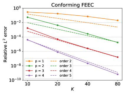
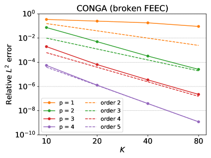
Figure 1: Convergence curves for the Hodge Laplace source problem, discretized with a conforming (left) and broken FEEC (right) method. For the latter, various penalization regimes lead to similar curves, as described in the text. On the horizontal axis we report the number of cells $K$ along each direction, hence $h=2\pi/K$; on the vertical axis we report the $L^{2}$ norm of the error, divided by the $L^{2}$ norm of the exact solution.

We next study the CONGA (broken FEEC) approximation of the eigenproblem (4.44). On the square $\Omega=]0,2\pi[^{2}$, the eigenvalues of the Hodge Laplacian operator $L^{1}=-\operatorname{{\bf grad}}\operatorname{div}+\operatorname{{\bf curl}}\operatorname{curl}$ with $D(L^{1})$ given by (5.26), read $\lambda_{\boldsymbol{n}}=\frac{1}{4}(n_{1}^{2}+n_{2}^{2})$ for ${\boldsymbol{n}}\in\mathbbm{N}^{2}$, with separable eigenmodes of the form

$$u_{1,{\boldsymbol{n}}}=\begin{pmatrix}\cos\big{(}\frac{n_{1}x_{1}}{2}\big{)}\sin\big{(}\frac{n_{2}x_{2}}{2}\big{)}\\ 0\end{pmatrix}\quad\text{ and }\quad u_{2,{\boldsymbol{n}}}=\begin{pmatrix}0\\ \sin\big{(}\frac{n_{1}x_{1}}{2}\big{)}\cos\big{(}\frac{n_{2}x_{2}}{2}\big{)}\end{pmatrix}$$

where we must of course discard the zero fields, and in particular the index ${\boldsymbol{n}}=(0,0)$. Note that each eigenvalue comes with an even multiplicity, namely 2 if $n_{1}=n_{2}$ or $n_{1}n_{2}=0$, or higher. In Figure 2 we show the eigenvalues of the discrete CONGA operator (4.45) corresponding to spaces of degree $p=2$ and different mesh sizes. On the left panel we show the first 40 eigenvalues of the operator associated with the penalization parameters (5.29). The convergence there seems to be rapid, which is confirmed in Figure 3 where the eigenvalue errors $\lvert\lambda_{\boldsymbol{n}}-\lambda_{{\boldsymbol{n}},h}\rvert$ are plotted in logscale for the same parameters. These results can be compared with the analog quantities corresponding to a penalization $\alpha_{h}=1$, shown on the right panels of Figure 2 and 3. For this weak penalization regime we see a clear issue: the first six eigenvalues do not converge, but rather stagnate around a value close to 1.22 which is related with the jump penalization operator $(I-P^{*}_{h})(I-P_{h})$. This spurious eigenvalue has actually a large multiplicity (indeed the 40 eigenvalues shown here are those which are closer to the exact ones, but not the smallest ones) and other runs have shown that it varies with the degree $p$.

Overall, these results provide a numerical validation of Theorems 4.10 and 4.15. We finally show in Figure 4 the non-zero eigenvalues and associated eigenvalue errors obtained with the unpenalized operator corresponding to the limit value $\alpha_{h}=0$. As expected the unpenalized operator has a large (spurious) kernel, but by plotting the first 40 non-zero eigenvalues we obtain curves which are virtually on top of those of the strongly penalized case, seen in the left panels of Figure 2 and 3. Thus, these numerical results suggest that the nontrivial discrete spectrum converges towards the exact one with no need of a stabilization. If true, this result would extend a similar one proven in [15] for the unpenalized CONGA approximation of the curl-curl eigenvalue problem. Although the unpenalized case is not covered by the analysis presented in this article, our explanation for this behaviour is that in the weakly penalized case the spurious eigenvalues are close to the correct ones, and their large multiplicity leads to a mixing of the spurious and correct eigenspaces. In the unpenalized case the spurious eigenmodes essentially correspond to the kernel of $L_{h,0}$, hence they are clearly separated from the correct ones which are associated with positive eigenvalues $\lambda_{h}=(\lVert d^{*}_{h}u_{h}\rVert^{2}+\lVert d_{h}u_{h}\rVert^{2})/\lVert u_{h}\rVert^{2}>0$. In particular the respective eigenspaces are orthogonal, owing to the symmetry of the discrete Hodge Laplacian operator.

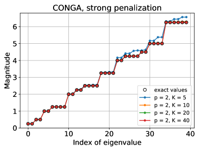
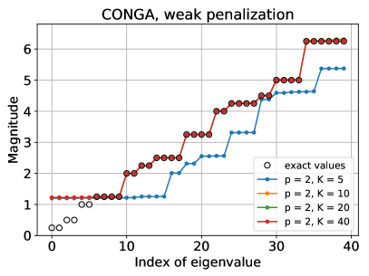
Figure 2: Discrete eigenvalues of the CONGA Hodge Laplacian operator on the square, with strong (left) and weak (right) penalization regimes, as discussed in the text.

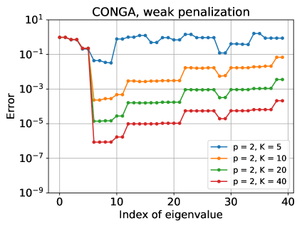
Figure 3: Eigenvalue errors for the CONGA Hodge Laplacian operator on the square, for the same parameters as in Figure 2.

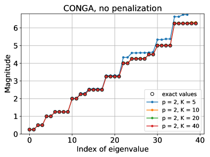
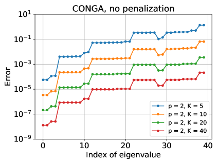
Figure 4: Positive eigenvalues and errors for the unpenalized ($\alpha_{h}=0$) CONGA Hodge Laplacian operator on the square.

6 Conclusion

In this article we have studied general discretizations of Hilbert complexes $(V,d)$ where the conformity constraint is relaxed while preserving most of the intrinsic stability and structure-preservation properties of conforming Finite Element Exterior Calculus (FEEC) discretizations. In our approach the nonconforming complexes $(V_{h},d_{h})$ rely on stable conforming discretizations, i.e. discrete subcomplexes $(V^{c}_{h},d)$ admitting a bounded cochain projection $\pi_{h}:V\to V^{c}_{h}$, and the discrete differential operators $d_{h}=dP_{h}$ are based on conforming projections $P_{h}:V_{h}\to V_{h}$ which are stable projection operators onto the underlying subcomplex $V^{c}_{h}=V_{h}\cap V$.

This broken FEEC approach has been originally introduced in the conforming/nonconforming Galerkin (CONGA) approximations to time-dependent Maxwell equations [15], where the curl-conformity constraint was relaxed while preserving the de Rham structure properties in the case of an exact sequence. Here we have extended this approach to the discretization of full Hilbert complexes with nontrivial harmonic spaces, and we have completed the construction with stable commuting projections $\tilde{\pi}_{h}$ for the dual (weak) discrete sequence. We have also studied the properties of the associated CONGA Hodge Laplacian operator, in particular we have shown that it has the same kernel as the underlying conforming FEEC Hodge Laplacian operator (namely, conforming discrete harmonic fields), provided an arbitrary stabilization term is used to handle the space nonconformities.

In a second part, we have studied the CONGA Hodge Laplace source and eigenvalue problems. Under stability and moment-preserving assumptions for the conforming projections we have shown that the source problem is well–posed, and we have derived a priori error estimates that allowed us to demonstrate the spectral correctness of the penalized CONGA Hodge Laplacian operator. This guarantees in particular that the latter is free of spurious eigenvalues.

In a third part we have applied our broken FEEC discretization method to polynomial finite elements where the cell-diagonal structure of the mass matrices naturally yields local discrete differential operators, both for the primal (strong) and dual (weak) sequences, as well as local $L^{2}$ stable dual commuting projection operators. Finally we have validated our theoretical study with numerical examples on a simple square domain, and we have assessed their dependency with respect to the stabilization parameter. We point out that these results have been extended to mapped spline elements on multi-patch non-contractible domains in a recent article [22] where CONGA schemes have been also proposed for several electromagnetic problems, including time-harmonic Maxwell and magnetostatic problems. Our results also seem to indicate that the CONGA Hodge Laplacian is spectrally correct in the absence of stabilization. This property however falls outside the scope of the present analysis, and remains a subject for further investigation.

References

• [1] Douglas N. Arnold, Pavel B. Bochev, Richard B. Lehoucq, Roy A. Nicolaides, and Mikhail Shashkov (eds.), Compatible spatial discretizations, The IMA Volumes in Mathematics and its Applications, vol. 142, Springer, New York, 2006, Papers from the IMA Hot Topics Workshop on Compatible Spatial Discretizations for Partial Differential Equations held at the University of Minnesota, Minneapolis, MN, May 11–15, 2004. MR 2256572
• [2] Douglas N. Arnold, Richard S. Falk, and Ragnar Winther, Finite element exterior calculus, homological techniques, and applications, Acta Numerica 15 (2006), 1–155 (English).
• [3]  , Finite element exterior calculus: From Hodge theory to numerical stability, Bull. Am. Math. Soc., New Ser. 47 (2010), no. 2, 281–354 (English).
• [4] Daniele Boffi, Fortin operator and discrete compactness for edge elements, Numerische Mathematik 87 (2000), no. 2, 229–246.
• [5]  , Compatible Discretizations for Eigenvalue Problems, Compatible Spatial Discretizations, Springer New York, New York, NY, 2006, pp. 121–142.
• [6]  , Finite element approximation of eigenvalue problems, Acta Numerica 19 (2010), 1–120 (English).
• [7] Daniele Boffi, Franco Brezzi, and M Fortin, Mixed finite element methods and applications, Springer Series in Computational Mathematics, vol. 44, Springer, 2013.
• [8] Daniele Boffi, Franco Brezzi, and Lucia Gastaldi, On the problem of spurious eigenvalues in the approximation of linear elliptic problems in mixed form, Mathematics of Computation 69 (2000), 121 – 140.
• [9] Alain Bossavit, Computational electromagnetism. Variational formulations, complementarity, edge elements, Orlando, FL: Academic Press, 1998 (English).
• [10] Haim Brezis, Functional analysis, Sobolev spaces and partial differential equations, Universitext, New York, NY: Springer, 2011 (English).
• [11] Annalisa Buffa, Ilaria. Perugia, and Tim Warburton, The Mortar-Discontinuous Galerkin Method for the 2D Maxwell Eigenproblem - Springer, Journal of Scientific Computing (2009).
• [12] Annalisa Buffa, Giancarlo Sangalli, and Rafael Vázquez, Isogeometric analysis in electromagnetics: B-splines approximation, Computer Methods in Applied Mechanics and Engineering 199 (2010), no. 17, 1143–1152.
• [13] Martin Campos Pinto, Constructing exact sequences on non-conforming discrete spaces, Comptes Rendus Mathematique 354 (2016), no. 7, 691–696.
• [14] Martin Campos Pinto, Katharina Kormann, and Eric Sonnendrücker, Variational framework for structure-preserving electromagnetic particle-in-cell methods, J. Sci. Comput. 91 (2022), no. 2, 39 (English), Id/No 46.
• [15] Martin Campos Pinto and Eric Sonnendrücker, Gauss-compatible Galerkin schemes for time-dependent Maxwell equations, Math. Comput. 85 (2016), no. 302, 2651–2685 (English).
• [16]  , Compatible Maxwell solvers with particles I: conforming and non-conforming 2D schemes with a strong Ampere law, The SMAI Journal of Computational Mathematics 3 (2017), 53–89. MR 3695788
• [17]  , Compatible Maxwell solvers with particles II: conforming and non-conforming 2D schemes with a strong Faraday law, The SMAI Journal of Computational Mathematics 3 (2017), 91–116. MR 3695789
• [18] Salvatore Caorsi, Paolo Fernandes, and Mirco Raffetto, On the convergence of Galerkin finite element approximations of electromagnetic eigenproblems, SIAM Journal on Numerical Analysis 38 (2000), no. 2, 580–607 (electronic).
• [19] Gary Cohen and Peter Monk, Gauss point mass lumping schemes for Maxwell’s equations, Numer. Methods Partial Differ. Equations 14 (1998), no. 1, 63–88 (English).
• [20] Herbert Egger and Bogdan Radu, A second-order finite element method with mass lumping for Maxwell’s equations on tetrahedra, SIAM J. Numer. Anal. 59 (2021), no. 2, 864–885 (English).
• [21] Marc Gerritsma, Edge functions for spectral element methods, Spectral and High Order Methods for Partial Differential Equations, Springer, Heidelberg, 2011, pp. 199–207.
• [22] Yaman Güçlü, Said Hadjout, and Martin Campos Pinto, A broken FEEC framework for electromagnetic problems on mapped multipatch domains, Journal of Scientific Computing 97 (2023), no. 2, 52.
• [23] Ralf Hiptmair, Finite elements in computational electromagnetism, Acta Numerica 11 (2002), 237–339 (English).
• [24] Michael Kraus, Katharina Kormann, Philip J. Morrison, and Eric Sonnendrücker, GEMPIC: Geometric electromagnetic particle-in-cell methods, Journal of Plasma Physics 83 (2017), no. 4.
• [25] Jasper Kreeft, Artur Palha, and Marc Gerritsma, Mimetic framework on curvilinear quadrilaterals of arbitrary order, 2011.
• [26] Jeonghun J. Lee, High order approximation of Hodge Laplace problems with local coderivatives on cubical meshes, ESAIM, Math. Model. Numer. Anal. 56 (2022), no. 3, 867–891 (English).
• [27] Jeonghun J. Lee and Ragnar Winther, Local coderivatives and approximation of Hodge Laplace problems, Math. Comput. 87 (2018), no. 314, 2709–2735 (English).
• [28] Peter Monk and Leszek Demkowicz, Discrete compactness and the approximation of Maxwell’s equations in $\mathbb{R}^{3}$, Math. Comput. 70 (2001), no. 234, 507–523 (English).
• [29] Nicolas Robidoux, Polynomial histopolation, superconvergent degrees of freedom and pseudo-spectral discrete Hodge operators, Unpublished, 2008.