Settling an old story: solution of the Thirring model in thimble regularization

Abstract

Thimble regularisation of lattice field theories has been proposed as a solution to the infamous sign problem. It is conceptually very clean and powerful, but it is in practice limited by a potentially very serious issue: in general many thimbles can contribute to the computation of the functional integrals. Semiclassical arguments would suggest that the fundamental thimble could be sufficient to get the correct answer, but this hypothesis has been proven not to hold true in general. A first example of this failure has been put forward in the context of the Thirring model: the dominant thimble approximation is valid only in given regions of the parameter space of the theory. Since then a complete solution of this (simple) model in thimble regularisation has been missing. In this paper we show that a full solution (taking the continuum limit) is indeed possible. It is possible thanks to a method we recently proposed which de facto evades the need to simulate on many thimbles.

1 Introduction

The lattice regularization of a Quantum Field Theory (QFT) enables access to non-perturbati-ve aspects of the theory by numerical simulations. On the lattice physical quantities are defined as high-dimensional integrals which can be computed via importance sampling by interpreting the factor $e^{-S}$ that appears in the integrands as a probability distribution. This technique has proven to be very effective to understand, for instance, the phenomenon of confinement in QCD. Unfortunately there are very interesting theories whose action $S$ is complex, so that $e^{-S}$ is not a well-defined probability distribution. This is the so-called sign problem and it affects for instance QCD at finite density. For this very reason the phase diagram of QCD remains largely unexplored by lattice simulations.

Not so long ago, following earlier work by Witten [1, 2], it was proposed that one could evade the sign problem by regularizing a QFT on Lefschetz thimbles [3, 4]. The idea is simple. After complexifying the degrees of freedom one can define a set of manifolds attached to the critical (stationary) points of the theory. These manifolds are called Lefschetz thimbles. The Lefschetz thimbles are a basis for the original integration circle in the homological sense, i.e. the original integrals can be decomposed to a linear combination of integrals over the thimbles. In other terms the thimble decomposition defines a convenient deformation of the original domain of integration (as a result the value of the integral does not change). It is a convenient deformation because on the thimbles the imaginary part of the action stays constant. Thus every contribution is free of the sign problem, apart from a residual phase coming from the orientation of the thimble in the embedding manifold. This gives rise to a residual sign problem, which is in practice found to be a (quite) milder one. Also, the coefficients appearing in the decomposition (the so-called intersection numbers) are integers and they can be zero, meaning that not all the thimbles do necessarily contribute.

Semiclassical arguments would suggest that the thimble attached to the critical point having the minimum real part of the action (aka the fundamental thimble) gives the dominant contribution. This contribution is expected to be further enhanced in the continuum limit. Since the theory formulated on a single thimble has the same symmetries and the same perturbative expansion as the original theory, it was conjectured that the contribution coming from the fundamental thimble could be considered a good approximation for the complete theory. This conjecture is known as the single-thimble dominance hypothesis. Soon it was discovered that this hypothesis holds true in some cases, but does not hold true in general. Various counter-examples have been found, such as the ($0$+$1$)-dimensional QCD [5] and heavy-dense QCD [6], where the single-thimble approximation fails. To our knowledge, the first counter-example that has been discovered is the one-dimensional Thirring model. In refs. [7, 8, 9, 10] it was shown that taking into account the fundamental thimble alone is not enough to reproduce the correct results, not even in the continuum limit. Indeed how to address the failure of the single-thimble approximation for this theory has been an open question that we want to settle in this paper. There is little doubt that a convenient thimble regularisation of the theory will work, but this is expected to take into account contributions from many thimbles and of course “How many?” is a key issue. We will show that we can indeed compute the solution of the theory by thimble regularisation (and the continuum limit can be taken). Quite interestingly, this will be most effectively achieved in a way that to a large extent evades the subtleties of collecting contributions from many thimbles.

The problem of collecting the contributions from more than one thimble is non-trivial. The contributions can be individually estimated by importance sampling, but they must be properly weighted in the thimble decomposition. A universal and satisfactory way to obtain the weight is to date still missing. This was a major motivation for the exploration of alternative formulations somehow inspired by thimbles, e.g. the holomorphic flow [10, 11] or various definitions of sign-optimised manifolds, possibly selected by deep-learning techniques [12, 13, 14, 15]. Still, some proposals for multi-thimbles simulations have been made in the literature [5, 6, 16, 17]. In particular, in ref. [6] we proposed a two-steps process in which one first computes the weights in the semiclassical approximation and then computes the relevant corrections. This worked fairly well for the simple version of heavy-dense QCD we had considered. Nonetheless it turned out that this method doesn’t work that well for the Thirring model. Therefore we turned back to the method we had thought of in ref. [5], where the weights are obtained by using a few known observables as normalization points. We also applied the method we have proposed in ref. [18] in which observables are reconstructed by merging via Padé approximants different Taylor series carried out around points where the single-thimble approximation is a good one. This last method proved to be more effective and it allowed to repeat the simulations towards the continuum limit.

The paper is organized as follows. In section 2 we discuss the strategy we’ve put in place to perform one-thimble simulations, in particular summarizing the algorithm we have adopted for the Monte Carlo integration. In section 3 we report the numerical results we have obtained for the Thirring model from one-thimble simulations. Not surprisingly we observe the failure of the single-thimble approximations as it was already reported in refs. [7, 8, 9, 10]. In section 4 we show how we can address the issue by collecting the contributions from the sub-dominant thimbles. The relative weight between the dominant and the sub-dominant thimbles is obtained by the method proposed in ref. [5]. Finally in section ref. 5 we apply the strategy outlined in ref. [18]. This strategy allowed to carry out the study of the continuum limit.

2 Monte Carlo integration on thimbles

The thimble decomposition for a given observable $\langle O\rangle$ can be stated as

$$\left\langle O\right\rangle\, =\,Z^{-1}\,\int dx\;e^{-S(x)}\,O(x)$$ (1a)

$$=\,{{\sum_{\sigma}\;n_{\sigma}\,e^{-i\,S_{I}(p_{\sigma})}\,\int_{\mathcal{J}_{\sigma}}dz\;e^{-S_{R}(z)}\;O(z)\;e^{i\,\omega(z)}}\over{\sum_{\sigma}\;n_{\sigma}\,e^{-i\,S_{I}(p_{\sigma})}\,\int_{\mathcal{J}_{\sigma}}dz\;e^{-S_{R}(z)}\;e^{i\,\omega(z)}}}$$ (1b)

$$=\,{{\sum_{\sigma}\;n_{\sigma}\,e^{-i\,S_{I}(p_{\sigma})}\,Z_{\sigma}\left\langle O\,e^{i\,\omega}\right\rangle_{\sigma}}\over{\sum_{\sigma}\;n_{\sigma}\,e^{-i\,S_{I}(p_{\sigma})}\,\,Z_{\sigma}\left\langle e^{i\,\omega}\right\rangle_{\sigma}}}$$ (1c)

Eq. 1a defines the physical quantity we want to calculate, where $x$ is a short-hand notation for the fields configurations and $S(x)=S_{R}(x)+iS_{I}(x)$ is the complex-valued action of the system.

In eq. 1b the real degrees of freedom have been complexified, i.e. $x\mapsto z$. The integrals at the numerator and at the denominator have been rewritten as linear combinations of integrals over the stable thimbles $\mathcal{J}_{\sigma}$ attached to the critical points $p_{\sigma}$ (in this context we call critical points the stationary points of the complexified action, i.e. the points such that $\partial_{z}S(p_{\sigma})=0$). The stable thimble attached to a given critical point $p_{\sigma}$ is the union of the solutions of the steepest-ascent (SA) equations stemming from the critical point,

$${{d}\over{dt}}z_{i}={{\partial\bar{S}}\over{\partial\bar{z}_{i}}}\mbox{ , \hskip 7.11317pt}z_{i}(-\infty)=p_{\sigma,i}\mbox{ . }$$ (2)

Along each SA path the real part of the action is always increasing. On the other hand the imaginary part of the action stays constant, therefore the expressions $e^{-i\,S_{I}(p_{\sigma})}$ have been factorized in front of the integrals. The $n_{\sigma}$ are integer coefficients known as intersection numbers. These count the number of intersections between the original integration contour and the unstable thimbles $\mathcal{K_{\sigma}}$, which are defined as the unions of the solutions of the steepest-descent (SD) equations leaving the critical point. Along each SD path the real part of the action is always decreasing. In eq. 1b a so-called residual phase $e^{i\,\omega(z)}$ appears in the integrals. This phase comes from the orientation of the thimble in the embedding manifold and it introduces a residual sign problem, though this is usually found to be a mild one.

In eq. 1c the thimble decomposition has been reformulated in a way that is amenable to numerical simulations. We have defined an expectation value on the thimble $\mathcal{J}_{\sigma}$,

$$\langle f\rangle_{\sigma}={{\int_{\mathcal{J}_{\sigma}}dz~{}f~{}e^{-S_{R}}}\over{\int_{\mathcal{J}_{\sigma}}dz~{}e^{-S_{R}}}}={{\int_{\mathcal{J}_{\sigma}}dz~{}f~{}e^{-S_{R}}}\over{Z_{\sigma}}}\mbox{ , }$$ (3)

that we plan to evaluate stochastically. Notice that in order to make use of the thimble decomposition, one has to carry out two tasks. In addition to computing the thimble contributions $\langle f\rangle_{\sigma}$ one also has to calculate their associated weights $Z_{\sigma}$. Now we summarize the procedure we have put in place to numerically compute $\langle f\rangle_{\sigma}$. This is all that is needed in the single-thimble approximation, where one only takes into account the contribution coming from the fundamental thimble. Later on we will also discuss the issue of computing the weights in a generic thimble decomposition.

By solving the Takagi’s problem for the Hessian of the action $H(S;z)$

$$H(S;p_{\sigma})\,v^{(i)}=\lambda_{i}\,\bar{v}^{(i)}$$

one can find a set of Takagi vectors $v^{(i)}$ and their associated Takagi values $\lambda_{i}$. The Takagi vectors are a basis for the tangent space at the critical point. After having fixed a normalization $\mathcal{R}$, the direction associated to a given (infinitesimal) displacement from the critical point (a sort of initial condition for a given SA path) can be expressed as $\sum n_{i}v^{(i)}$, with $\hat{n}\in\mathcal{S}^{n-1}_{\mathcal{R}}$, where $\mathcal{S}^{n-1}_{\mathcal{R}}$ is the $(n-1)$-dimensional hypersphere of radius $\mathcal{R}$. A point on the thimble can be singled out by the initial direction of the flow $\hat{n}$ and by the integration time $t$,

$$z\in\mathcal{J_{\sigma}}\leftrightarrow(\hat{n},t)\in\mathcal{S}^{n-1}_{\mathcal{R}}\times\mathbb{R}\mbox{ . }$$

Let’s first consider the denominator of eq. 3, which we somehow improperly refer to as a partition function. We can rewrite it in terms of the integration measure $\mathcal{D}\hat{n}=\prod_{k}dn_{k}\delta(|\hat{n}|^{2}-\mathcal{R}^{2})$,

$$Z_{\sigma}=\int_{\mathcal{J}_{\sigma}}dz~{}e^{-S_{R}(z)}=\int\mathcal{D}\hat{n}~{}\int dt~{}\Delta_{\hat{n}}^{\sigma}(\hat{n},t)~{}e^{-S_{R}(\hat{n},t)}\equiv\int\mathcal{D}\hat{n}~{}Z_{\hat{n}}^{\sigma}\mbox{ , }$$

where $\Delta_{\hat{n}}^{\sigma}(\hat{n},t)$ is a leftover from the change of variables. An explicit expression for $\Delta_{\hat{n}}^{\sigma}(\hat{n},t)$ was worked out in ref. [19]. One finds the following expression for the partial partition function,

$$Z_{\hat{n}}^{\sigma}=2(\sum_{i}\lambda_{i}n_{i}^{2})\int dt~{}e^{-S_{eff}(\hat{n},t)}\mbox{ . }$$

Notice that we have defined the effective action $S_{eff}(\hat{n},t)=S_{R}(\hat{n},t)-log|det~{}V(\hat{n},t)|$ from the real part of the action $S_{R}(\hat{n},t)$ and the matrix $V(\hat{n},t)$ having as columns the basis vectors of the tangent space at the time $t$. In order to compute the partial partition function one has to parallel transport the basis vectors along the flow starting from the critical point, where a basis is known (the Takagi vectors). This requires integrating the parallel transport equations

$${{dV_{j}^{(h)}}\over{dt}}=\sum_{i}\overline{V}_{i}^{(h)}\overline{\partial^{2}_{z_{i}z_{j}}S}\mbox{ . }$$ (4)

The partial partition function can be interpreted as the contribution to the partition function coming from an entire SA path. Similarly for the numerator one finds

$$\int_{\mathcal{J}_{\sigma}}dz~{}f~{}e^{-S_{R}(z)}=\int\mathcal{D}\hat{n}~{}f_{\hat{n}}$$

$$f_{\hat{n}}=2(\sum_{i}\lambda_{i}n_{i}^{2})\int dt~{}f(\hat{n},t)~{}e^{-S_{eff}(\hat{n},t)}\mbox{ . }$$

All in all the expectation value $\langle f\rangle_{\sigma}$ becomes

$$\langle f\rangle_{\sigma}={{\int\mathcal{D}\hat{n}~{}f_{\hat{n}}}\over{Z_{\sigma}}}=\int\mathcal{D}\hat{n}~{}{{Z_{\hat{n}}^{\sigma}}\over{Z_{\sigma}}}~{}{{f_{\hat{n}}}\over{Z_{\hat{n}}^{\sigma}}}$$

This expectation value can be computed by importance sampling, sampling entire SA paths $\propto{{Z_{\hat{n}}^{\sigma}}\over{Z_{\sigma}}}$ and estimating the result from the sample mean ${{1}\over{N}}\sum_{\hat{n}}{{f_{\hat{n}}}\over{Z_{\hat{n}}}}$. All in all, in the following we have to think of a SA (parametrised by a direction $\hat{n}$) as we think of a configuration in a standard Monte Carlo. The algorithm proceeds in two steps.

1. First we make a Metropolis proposal starting from the previous configuration $\hat{n}$. The proposal is generated by making $N$ consecutive rotations in planes defined by random directions. That is we pick two random integers $i\neq j$ and we perform a rotation in the place singled out by the $i$-th and the $j$-th direction, i.e. we (propose an) update $(n_{i},n_{j})\mapsto(n_{i}^{\prime},n_{j}^{\prime})$ subject to the normalization condition. Then we pick another random integer $k\neq j$ and we perform a rotation in the plane singled out by the $j$-th and the $k$-th direction. We iterate until we have made $N$ rotations. Each rotation is obtained by parametrizing $(n_{i},n_{j})$ as

   $$\begin{cases}n_{i}=\sqrt{C}~{}sin(\phi)\\ n_{j}=\sqrt{C}~{}cos(\phi)\\ \end{cases}$$

   and proposing

   $$\begin{cases}n^{\prime}_{i}=\sqrt{C}~{}sin(\phi+\phi_{0})\\ n^{\prime}_{j}=\sqrt{C}~{}cos(\phi+\phi_{0})\mbox{ , }\\ \end{cases}$$

   where $C=n_{i}^{2}+n_{j}^{2}$ and $\phi_{0}$ has been uniformly extracted in $[-\alpha,\alpha]$.

2. Once we have proposed a new configuration $\hat{n}^{\prime}$, we perform a Metropolis accept/reject test by accepting the proposal with probability $P_{acc}(\hat{n}^{\prime}\leftarrow\hat{n})=min\left(1,{{Z_{\hat{n}^{\prime}}^{\sigma}}\over{Z_{\hat{n}}^{\sigma}}}\right)$. Since the Metropolis proposal is symmetric, this is enough to satisfy the detailed balance principle and the Markov chain will converge to the targeted probability distribution ${{Z_{\hat{n}}^{\sigma}}\over{Z_{\sigma}}}$.

The key ingredients that we need to compute are the partial partition function $Z_{\hat{n}}$ and the (contribution from the current SA path to the) observable $f_{\hat{n}}$. These are time integrals whose computation requires to integrate the differential equations for both the fields and the basis vectors given in eq. 2 and eq. 4 starting from an initial condition close to the critical point,

$$\begin{cases}z=z_{\sigma}+n_{i}e^{\lambda_{i}t}v^{(i)}\\ V^{(h)}=v^{(h)}e^{\lambda_{h}t}\mbox{ . }\end{cases}$$

Actually in our calculations we integrate in action instead of integrating in time. Since the real part of the action is monotonic in time, one can make the change of variable

$${{dS_{R}}\over{dt}}={{1}\over{2}}{{d}\over{dt}}(S+\overline{S})=|\nabla S|^{2}\mapsto dt=dS_{R}~{}|\nabla S|^{-2}=ds~{}|\nabla S|^{-2}\mbox{ . }$$

In the last step we have also defined a second change of variable $s=S_{R}-S_{R}(z_{\sigma})$. In terms of $s$, the differential equations for the fields and the basis become

$${{dz_{i}}\over{ds}}=|\nabla S|^{-2}~{}{{\partial\overline{S}}\over{\partial\overline{z}_{i}}}$$

$${{dV_{j}^{(h)}}\over{ds}}=|\nabla S|^{-2}~{}\sum_{i}\overline{V}_{i}^{(h)}\overline{\partial^{2}_{z_{i}z_{j}}S}\mbox{ . }$$

The change of variable is also performed for the time integrals defining $Z_{\hat{n}}$ and $f_{\hat{n}}$, yielding

$$Z_{\hat{n}}=2\sum_{i}\lambda_{i}n_{i}^{2}e^{-S_{R}(z_{\sigma})}\int_{0}^{\infty}ds~{}|\nabla S|^{-2}~{}e^{-s+log|det~{}V(s)|}$$ (5)

$$f_{\hat{n}}=2\sum_{i}\lambda_{i}n_{i}^{2}e^{-S_{R}(z_{\sigma})}\int_{0}^{\infty}ds~{}f~{}|\nabla S|^{-2}~{}e^{-s+log|det~{}V(s)|}\mbox{ . }$$

The advantage is twofold. First, the integration in action has the effect of decreasing the number of iterations required to reach convergence. Second, one can immediately recognize from eqs. 5 that the integrals can be calculated using the Gauss-Laguerre quadrature, i.e.

$$\int_{0}^{\infty}f(x)e^{-x}dx=\sum w_{i}f(x_{i})\mbox{ . }$$

where $\{x_{i}\}$ and $\{w_{i}\}$ are the quadrature points and their associated weights. The calculation of the determinant (which is computationally quite expensive) is required only at the quadrature points.

3 One-thimble simulations

We now discuss the thimble regularization of the one-dimensional Thirring model. As we have remarked in the introduction, historically this is one of the very first examples that have shown the inadequacy of the single-thimble approximation (see refs [7, 8, 9, 10]). The lattice action for this theory can be written down as

$$S=\beta\sum_{n=1\ldots L}(1-cos(\phi_{n}))-log~{}det~{}D\mbox{,}$$

where $det~{}D={{1}\over{2^{L-1}}}\left(cosh(L\hat{\mu}+i\sum_{n}\phi_{n})+cosh(L~{}asinh(\hat{m}))\right)$ is the fermionic determinant. The parameters $\hat{\mu}=\mu a$ and $\hat{m}=ma$ are respectively the chemical potential and the fermion mass in lattice units, $\beta=(2g^{2}a)^{-1}$ is the inverse coupling constant and $\phi_{n}$ is a scalar field discretized on a one-dimensional lattice of length $L$. The theory features a sign problem originating from the fermionic determinant, which is complex at finite $\hat{\mu}$.

An analytical solution is known for the partition function. This is given in term of the modified Bessel functions of the first kind $I_{n}(x)$,

$$Z={{1}\over{2^{L-1}}}e^{-L\beta}\left[I_{1}(\beta)^{L}cosh(L\hat{\mu})+I_{0}(\beta)^{L}cosh(L~{}asinh(\hat{m}))\right]\mbox{ . }$$

From the partition function one can derive closed-form expressions for the physical observables, such the scalar condensate $\langle\bar{\chi}\chi\rangle$ and the fermion density $\langle n\rangle$,

$$\langle\bar{\chi}\chi\rangle={{1}\over{L}}{{\partial log~{}Z}\over{\partial\hat{m}}}={{1}\over{cosh(asinh(\hat{m}))}}{{I_{0}(\beta)^{L}sinh(L~{}asinh(\hat{m}))}\over{I_{1}(\beta)^{L}cosh(L\hat{\mu})+I_{0}(\beta)^{L}cosh(L~{}asinh(\hat{m}))}}\mbox{ . }$$

$$\langle n\rangle={{1}\over{L}}{{\partial log~{}Z}\over{\partial\hat{\mu}}}={{I_{1}(\beta)^{L}sinh(L\hat{\mu})}\over{I_{1}(\beta)^{L}cosh(L\hat{\mu})+I_{0}(\beta)^{L}cosh(L~{}asinh(\hat{m}))}}$$

A solution by numerical methods, on the other hand, is difficult to obtain because of the sign problem. In this paper we explore the feasibility of using the thimble regularization method to study the Thirring model. The first step consists in complexifying the degrees of freedom. In this case, each real degree of freedom $\phi_{n}$ is replaced by a complex degree of freedom $z_{n}$. The action is now given in terms of $z_{n}$,

$$\beta\sum_{n=1\ldots L}(1-cos(z_{n}))-log~{}detD\mbox{ , }$$

where $detD={{1}\over{2^{L-1}}}\left(cosh(L\hat{\mu}+i\sum_{n}z_{n})+cosh(L~{}asinh(\hat{m}))\right)$. The critical points of the theory are found by requiring a vanishing gradient,

$${{\partial S}\over{\partial z_{n}}}=\beta sin(z_{n})-i~{}{{sinh(L\hat{\mu}+i\sum_{i}z_{i})}\over{cosh(L\hat{\mu}+i\sum_{i}z_{i})+cosh(L~{}asinh(\hat{m}))}}=0\mbox{ . }$$ (6)

From this condition one can see that $sin(z_{n})$ takes for all $n=1\ldots L$ always the same value, which we denote by $sin(z)$ and which depends on $z_{n}$ only through the sum $\sum_{n}z_{n}$. Therefore the critical points are given by field configurations where $z_{i}=z$ for any $i$ but a number $n_{-}$ of lattice points where $z_{i}$ can take the value $\pi-z$ (without changing $sin(z_{n})$). For a fixed $n_{-}$ the values admitted for $z$ are found by numerically solving

$$sin(z)={{i}\over{\beta}}{{sinh(L\hat{\mu}+i(L-2n_{-})z+in_{-}\pi)}\over{cosh(L\hat{\mu}+i(L-2n_{-})z+in_{-}\pi)+cosh(L~{}asinh(\hat{m}))}}\mbox{ . }$$ (7)

This equation follows directly from eq. 6. For instance let’s consider the critical points in the $n_{-}=0$ sector, which are expected to give the leading contributions [8]. The solutions corresponding to the parameters $L=4$, $\beta=1$ and $ma=1$ are graphically shown in fig. 1. The top left figure shows the solutions for $z$ of eq. 7, while the top right figure shows how they move when we add a finite chemical potential.

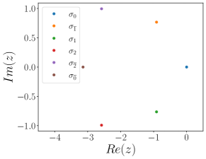
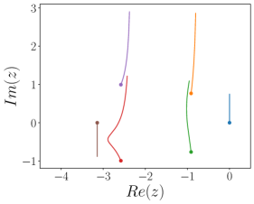
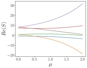
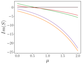
Figure 1: Critical points for $L=4$, $\beta=1$ and $ma=1$: solutions for $\hat{\mu}=0$ (top left), solutions for $\hat{\mu}\in[0.0,~{}2.0]$ (top right), real part of the action as a function of $\hat{\mu}$ (bottom left) and imaginary part of the action as a function of $\hat{\mu}$ (bottom right).

Notice that only the left complex half-plane is shown. Since eq. 7 is invariant under $z\mapsto-\bar{z}$, if $z$ defines a critical point so does $-\bar{z}$. Therefore each critical point $\sigma_{i}$ has a counterpart $\sigma_{-i}$ in the right complex half-plane. However these mirrored critical point do not give rise to independent contributions. Indeed the action displays a symmetry $S(-\bar{z})=\overline{S(z)}$ which ensures that the thimble contributions from the member of each pair $\sigma_{i}$, $\sigma_{-i}$ are conjugate contributions.

If we look at the bottom left picture of fig. 1 we can see that the fundamental thimble, the one attached to the critical point having the minimum (real part of the) action, is $\mathcal{J}_{\sigma_{0}}$. Actually from some chemical potential $\mu_{0}$ onwards the critical point $\sigma_{\bar{1}}$ has an even lower (real part of the) action, but since this is also lower than the minimum real part of the action on the original domain, the thimble attached to this critical point cannot appear in the thimble decomposition.

In fig. 2 we show the numerical results obtained from numerical simulations performed on the fundamental thimble $\mathcal{J}_{\sigma_{0}}$ for different values of $\beta=1.0$, $1.5$, $2.0$, $4.0$. At strong couplings (i.e. at low $\beta$) the single-thimble approximation yields the wrong results, at least for high chemical potentials. This does not come as a surprise (it is exactly what other authors found previously) and shows that the contribution from the sub-dominant thimbles cannot be neglected.

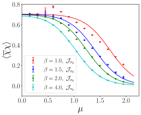
Figure 2: Scalar condensate for $L=4$, $\beta=1.0$, $1.5$, $2.0$, $4.0$ and $ma=1$: results from one-thimble simulations on $\mathcal{J}_{\sigma_{0}}$.

4 Multi-thimble simulations

The reason why the single-thimble approximation fails is that, when the chemical potential is increased starting from zero, different Stokes phenomena take place and the thimble decomposition changes. As a result thimbles other than the fundamental one need to be taken into account at high chemical potentials, even though at zero chemical potential the contribution from the fundamental thimble $\mathcal{J}_{\sigma_{0}}$ is the only non negligible one.

All in all the sub-dominant contribution that one has to take into account is the one from the thimble $\mathcal{J}_{\sigma_{1}}$, which enters the decomposition at $\hat{\mu}\approx 0.56$. Indeed at this chemical potential the imaginary parts of the action at $\sigma_{0}$ and $\sigma_{1}$ are the same, as shown in the bottom right picture of fig. 1. This is a necessary condition for a Stokes phenomenon, that indeed happens. For a very nice and thorough analysis of the Stokes phenomena and their consequences on the thimble decomposition, we refer the reader to ref. [8].

In order to properly collect the contributions from the fundamental thimble $\mathcal{J}_{\sigma_{0}}$ and the sub-dominant thimble $\mathcal{J}_{\sigma_{1}}$, we have to determine the relative weights of the two contributions. The approach we took is the one we’ve followed for ($0$+$1$)-dimensional QCD. Since we are considering only two independent thimble contributions, the expectation value of a generic observable $O$ can be written as

$$\langle O\rangle={{n_{0}e^{-iS_{I}(z_{0})}Z_{0}\langle Oe^{i\omega_{0}}\rangle_{0}+n_{12}e^{-iS_{I}(z_{12})}Z_{12}\langle Oe^{i\omega_{12}}\rangle_{12}}\over{n_{0}e^{-iS_{I}(z_{0})}Z_{0}\langle Oe^{i\omega_{0}}\rangle_{0}+n_{12}e^{-iS_{I}(z_{12})}Z_{12}\langle Oe^{i\omega_{12}}\rangle_{12}}}\mbox{ . }$$

Here we use the subscript $12$ to denote quantities that refer to the critical points $\sigma_{1}$ and $\sigma_{-1}$. As we have already observed these critical points give rise to conjugate contributions (whose sum is purely real). When $\mathcal{J}_{\sigma_{1}}$ enters the thimble decomposition, so does $\mathcal{J}_{\sigma_{-1}}$, but we have only one independent contribution. Now if we divide both the numerator and the denominator by $n_{0}e^{-iS_{I}(z_{0})}Z_{0}$ we obtain

$$\langle O\rangle={{\langle Oe^{i\omega_{0}}\rangle_{0}+\alpha\langle Oe^{i\omega_{12}}\rangle_{12}}\over{\langle e^{i\omega_{0}}\rangle_{0}+\alpha\langle e^{i\omega_{12}}\rangle_{12}}}\mbox{ . }$$

where $\alpha={{n_{12}e^{-iS_{I}(z_{12})}Z_{12}}\over{n_{0}e^{-iS_{I}(z_{0})}Z_{0}}}$. Since $\alpha$ only depends on the thimble structure of the theory, we can determine it by taking some observable $\tilde{O}$ as a normalization point and then use such value to calculate any other observable.

For the Thirring model we fixed $\alpha$ from the (analytical solution of the) number density and we used it to calculate the scalar condensate. The numerical results are shown in fig. 3. The results are now in agreement with the analytical solution: the contribution from the sub-dominant thimble fully accounts for the discrepancies observed in the results from one-thimble simulations (and that’s why we could make a long story short earlier, when we said that the sub-dominant contribution that one has to take into account is the one from the thimble $\mathcal{J}_{\sigma_{1}}$). Notice that the statistical errors are quite large for $\hat{\mu}\approx 0.6\div 0.75$, this is in part due to cancellations in the calculation of $\alpha$ and in part due to numerical difficulties in sampling the non-dominant thimble. The partial partition function (i.e. the probability distribution for importance sampling) shows sharp spikes in some regions of $n_{0}$ (i.e. the initial direction of the SA path on the tangent space along the Takagi vector having the largest Takagi value). Within these regions the partial partition function varies by several order of magnitude and this makes it difficult to keep a good acceptance ratio. Moreover for $\mathcal{J}_{\sigma_{1}}$ the regions are also so thin that the regions of interest cannot represented in double precision and quadruple precision is needed in the simulations, with a noticeable impact on the performance of the code. An example of this last issue is shown in fig. 4, where the logarithm of the partial partition function of $\mathcal{J}_{\sigma_{1}}$ is shown as a function of $n_{0}$ for a $L=2$ lattice.

In the next section we will study the Thirring model using a strategy that will turn out to be much more effective, since (a) it does need to take a known result as a normalisation point and (b) it does not require to sample the sub-dominant thimble.

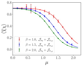
Figure 3: Scalar condensate for $L=4$, $\beta=1.0$, $1.5$, $2.0$ and $ma=1$: results from multi-thimble simulations on $\mathcal{J}_{\sigma_{0}}$ and $\mathcal{J}_{\sigma_{\pm 1}}$.

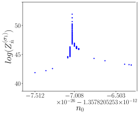
Figure 4: Logarithm of the partial partition function for the critical point $\sigma_{1}$. This is plotted as a function of $n_{0}$, i.e. the initial direction of the SA path on the tangent space along the Takagi vector having the largest Takagi value. Parameters: $L=2$, $\beta=1$ and $ma=1$.

5 Taylor expansions on the fundamental thimble

In this section we follow the approach we proposed in ref. [18] (the interested reader is referred to it for further details on the method itself). The main idea is that we can by-pass the need for multi-thimble simulations by calculating multiple Taylor expansions around points where the single-thimble approximation holds true. As a consequence, the coefficients of such expansions can be computed by one-thimble simulations. The method relies on the fact that while the thimble decomposition can be (highly) discontinuous as we sample different regions in the parameter space of the theory, physical observables (in general) are not. Our strategy is to take advantage of the single-thimble approximation holding true in given regions and bridge these different (disjoint) regions by Taylor expansions. Actually it turns out that the most efficient way to bridge these different regions is by Padé approximants. As a side-effect, having computed Padé approximants, we are able to probe the analytical structure of the observables, i.e. we can locate their singularities. This makes the approach a very powerful tool for theoretical investigations, with applications beyond thimble regularization itself. In a more general framework, one could say that bridging different regions by Padé approximants can be an effective way of studying the phase diagram of a theory for which direct computations can be approached only in given regions of the parameter space. Indeed such a strategy can be e.g. applied to lattice QCD at imaginary chemical potential [20, 21].

From a numerical point of view the method of [18] proved to be quite effective in our case. It allowed to study the Thirring model for (much) larger/finer lattices than the (modest) $L=4$ lattice we have considered in the previous sections.

Let’s start by studying the theory using $L=8$, $\beta=1$ and $ma=2$ as parameters. We need a few expansion points where the Taylor expansion can be calculated by one-thimble simulations:

1. As a first point we selected ${{\mu}\over{m}}=0.4$. This choice can be understood from a simple argument. The range of $S_{I}$ on the real domain of integration is limited. As a result, from explicit computation of $S_{I}^{\sigma}({{\mu}\over{m}})$ we can conclude that below a given value ${{\mu_{0}}\over{m}}$ of the chemical potential there are only two unstable thimbles that can intersect the real domain of integration. These are the one attached to the fundamental critical point $\sigma_{0}$ and the one attached to the critical point $\sigma_{\bar{0}}$. But the contribution from $\mathcal{J}_{\sigma_{\bar{0}}}$ can be neglected, as $S_{R}(\sigma_{\bar{0}})\gg S_{R}(\sigma_{0})$.

2. As a second point we selected ${{\mu}\over{m}}=1.4$. For this value of the chemical potential, all but three the critical points other than the fundamental one have $S_{R}(\sigma)\gg S_{R}(\sigma_{0})$. Hence we can neglect them. We denote the three remaining critical points by $\sigma_{1}$, $\sigma_{\bar{1}}$ and $\sigma_{\bar{2}}$. Two of them (namely $\sigma_{\bar{1}}$ and $\sigma_{\bar{2}}$) have a real part of the action $S_{R}$ less than the minimum $S_{R}^{min}$ of the real action on the original domain of integration. Hence their unstable thimble cannot intersect the original domain of integration. As for $\sigma_{1}$ one can explicitly check that the attached unstable thimble does not intersect the original domain of integration. See the top picture of fig. 5. The critical point $\sigma_{0}$ is represented by the green point sitting at $Re(z)=0$. The critical point $\sigma_{1}$ is represented by the closest green point to $\sigma_{0}$ to the left. The unstable thimbles are displayed in magenta.

3. The very same reasoning applied to ${{\mu}\over{m}}=0.4$ and ${{\mu}\over{m}}=1.4$ can be applied to ${{\mu}\over{m}}=0$ and ${{\mu}\over{m}}=1.8$ (actually at ${{\mu}\over{m}}=0$ there is no sign problem and thimble regularization is not even needed).

We have computed by one-thimble simulations the Taylor coefficients for the scalar condensate at ${{\mu}\over{m}}=0.4$ and ${{\mu}\over{m}}=1.4$ respectively up to orders $2$ and $5$. Then we have constructed a (multi-points) Padé approximation using these coefficients as inputs, adding as extra constraints the coefficients of order $0$ at the boundaries of the region we have considered, i.e. ${{\mu}\over{m}}=0$ and ${{\mu}\over{m}}=1.8$. These extra constraints were also calculated by one-thimble simulations.

The results are shown in the bottom left picture of fig. 5. The expansion points are displayed as black points. The numerical results from the Padé approximants are displayed in black (with error bars): they are in good agreement with the analytical solution (the black line). The bottom right picture of fig. 5 shows the expansion points (the black points) on the complex ${{\mu}\over{m}}$ plane. The picture also shows the pole of the approximant (the blue point) and the true singularity of the observable (the green point). The first matches quite well the latter.

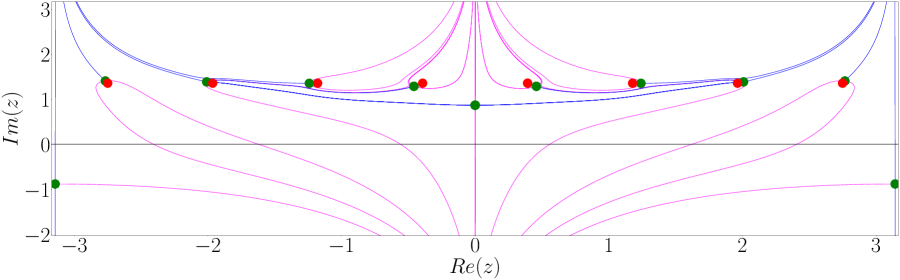
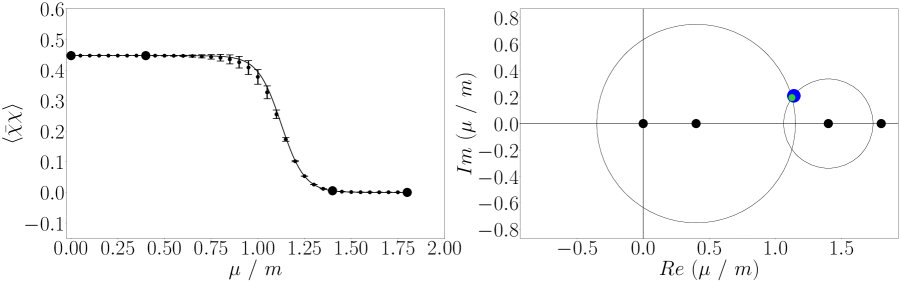
Figure 5: The top picture shows the thimble structure for $L=8$, $\beta=1.0$ and $ma=2$ at ${{\mu}\over{m}}=1.4$. The critical points are represented by the green points, while the stable and unstable thimbles are displayed in blue and magenta. The critical point $\sigma_{0}$ is the one sitting at $Re(z)=0$ and the critical point immediately on the left is $\sigma_{1}$. The unstable thimble attached to the former intersects the original domain of integration (the real axis), while the unstable thimble attached to the latter does not. The bottom left picture shows the results from Padé as black error bars, which are in very good agreement with the expectations from the analytical solution (represented by the black solid line). The expansion points are also shown as black points. In the bottom right picture the expansion points are displayed on the complex ${{\mu}\over{m}}$ plane. On top of these are also shown the singularity of the condensate (the green point) and the stable pole of the Padé approximant (the blue point).

Finally the simulations have been repeated towards the continuum limit. For this theory the continuum limit is reached by increasing $L={{1}\over{Ta}}$ and $\beta={{1}\over{2g^{2}a}}$ while keeping fixed the dimensionless products $L\hat{m}$ and $\beta\hat{m}$. In particular we kept constant $L\hat{m}=16$ and $\beta\hat{m}=2$. The parameters used in the simulations are summarized in tab. 1.

For the finer lattices we proceeded as we did for the $L=8$ lattice. We selected two suitable expansion points and we calculated the Taylor coefficients up to order $2$ and $5$ by one-thimble simulations. As extra constraints we also calculated the coefficients of order $0$ at the boundaries of the $\hat{\mu}$ range. These data were used as inputs to construct the Padé approximants. For the $L=32,64$ lattices the statistical error on the $5$th order Taylor coefficient was quite large and this resulted in a large indetermination on the Padé approximant itself. Fortunately in building our (multi-points) Padé approximants we have two different handles that we can make use of: one handle is the order of the Taylor expansions, the second one is the number of expansion points. For the $L=32,64$ lattices we decided to use an additional extra constraint in the low $\hat{\mu}$ region in place of the $5$th order Taylor coefficient.

The numerical results are shown in fig. 6. The bottom left and bottom right pictures show how the Padé approximants (the colored error bars) converge to the analytical solution (the red line) as we gradually increase the order of the Taylor coefficients calculated at the two (central) expansion points. Specifically these pictures illustrate what happens in the two different cases ($L=16$ and $L=64$) where respectively two and three extra constraints were used and the highest order that has been calculated in the Taylor expansion was respectively $5$ and $4$.

The top picture of fig. 6 summarizes the results we have obtained for all the lattices. Different colors denote different lattices. The analytical solutions are drawn as colored solid lines. The results from the simulations are in good agreement with the analytical solutions and the statistical error are well under control up to $L=64$.

$L$	$\beta$	$ma$
$8$	$1.0$	$2.00$
$16$	$2.0$	$1.00$
$32$	$4.0$	$0.50$
$64$	$8.0$	$0.25$

Table 1: Parameters used for the continuum limit analysis ($L\hat{m}=16$, $\beta\hat{m}=2$).

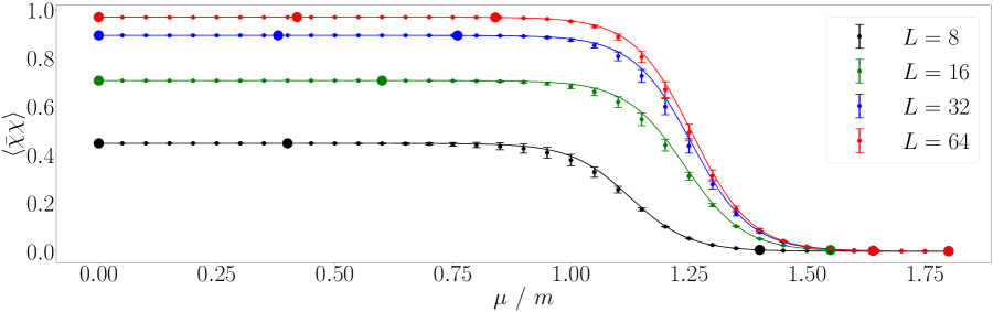
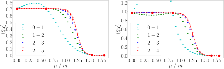
Figure 6: Results from the continuum limit analysis ($L\hat{m}=16$, $\beta\hat{m}=2$). The bottom left and bottom right pictures show how the Padé approximants converge to the correct solution for the $L=16$ and $L=64$ lattices. The expansion points are shown as red points. Different colors are used to denote the Padé approximants obtained by using a gradually increasing order of the Taylor coefficients for the two central expansion points. Respectively two and three extra constraints on the $0$th order Taylor coefficients were used for the two lattices and the highest order Taylor coefficient that was calculated is respectively $5$ and $4$. The top picture summarizes the results we obtained in our analysis. Different colors correspond to different lattice sizes. The analytical solutions are denoted by the colored solid lines.

6 Conclusions

The Thirring model has been extensively studied as a playground to test our ability to tackle finite-density theories plagued by a sign problem. This work aimed at settling an old story: is the thimble approach really failing for the (supposedly simple) Thirring model?
Thimble regularisation of lattice field theories is a conceptually nice solution to the sign problem, but it can be strongly limited by the need for multi-thimbles simulations. The Thirring model has indeed been a first example of the failure of the simplest application of the thimble approach, i.e. the one based on simulations on the dominant thimble alone. While there was little doubt of the conceptual solution to this failure (other thimbles provide an important contribution), an explicit proof of this has been till now missing. We showed that by keeping into account more contributions (on top of the dominant thimble) the (known) analytical solution can indeed be reconstructed. While this is conceptually clean, it is from a numerical point of view quite cumbersome. As a result, the computations we reported on were restricted to a system of modest size.
There is nevertheless a more powerful method to achieve the result we were interested in, which in the end avoids multi-thimbles simulations. We showed that we could successfully take the continuum limit in the computation of the Thirring model making use of the recently introduced method of computing Taylor expansions on thimbles. After calculating multiple Taylor expansions around points where the single-thimble approximation holds true, we could bridge these different (disjoint) regions by computing (multi-points) Padé approximants. The latter also gave us access to the singularity structure of the theory. While this settles the old story of the Thirring model in the thimble approach, at the same time suggests that a similar strategy can be successfully applied to problems beyond thimbles. Bridging different regions by Padé approximants can be an effective way of studying the phase diagram of a theory for which direct computations can be approached only in given regions of the parameter space.

References

- [1] E. Witten, Analytic Continuation Of Chern-Simons Theory, AMS/IP Stud. Adv. Math. 50, 347 (2011) [arXiv:1001.2933 [hep-th]].
- [2] E. Witten, A New Look At The Path Integral Of Quantum Mechanics, arXiv:1009.6032 [hep-th].
- [3] M. Cristoforetti et al. [AuroraScience Collaboration], New approach to the sign problem in quantum field theories: High density QCD on a Lefschetz thimble, Phys. Rev. D 86 (2012) 074506 [arXiv:1205.3996 [hep-lat]].
- [4] H. Fujii, D. Honda, M. Kato, Y. Kikukawa, S. Komatsu and T. Sano, Hybrid Monte Carlo on Lefschetz thimbles - A study of the residual sign problem, JHEP 1310 (2013) 147 [arXiv:1309.4371 [hep-lat]].
- [5] F. Di Renzo and G. Eruzzi, One-dimensional QCD in thimble regularization, Phys. Rev. D 97, no. 1, 014503 (2018) doi:10.1103/PhysRevD.97.014503 [arXiv:1709.10468 [hep-lat]].
- [6] K. Zambello and F. Di Renzo, Towards Lefschetz thimbles regularization of heavy-dense QCD, PoS LATTICE 2018, 148 (2018) doi:10.22323/1.334.0148 [arXiv:1811.03605 [hep-lat]].
- [7] H. Fujii, S. Kamata and Y. Kikukawa, Monte Carlo study of Lefschetz thimble structure in one-dimensional Thirring model at finite density, JHEP 1512 (2015) 125 Erratum: [JHEP 1609 (2016) 172] doi:10.1007/JHEP12(2015)125, 10.1007/JHEP09(2016)172 [arXiv:1509.09141 [hep-lat]].
- [8] H. Fujii, S. Kamata and Y. Kikukawa, Lefschetz thimble structure in one-dimensional lattice Thirring model at finite density, JHEP 1511 (2015) 078 Erratum: [JHEP 1602 (2016) 036] doi:10.1007/JHEP02(2016)036, 10.1007/JHEP11(2015)078 [arXiv:1509.08176 [hep-lat]].
- [9] A. Alexandru, G. Basar and P. Bedaque, Monte Carlo algorithm for simulating fermions on Lefschetz thimbles, Phys. Rev. D 93 (2016) no.1, 014504 doi:10.1103/PhysRevD.93.014504 [arXiv:1510.03258 [hep-lat]].
- [10] A. Alexandru, G. Basar, P. F. Bedaque, G. W. Ridgway and N. C. Warrington, Sign problem and Monte Carlo calculations beyond Lefschetz thimbles, JHEP 05 (2016), 053 doi:10.1007/JHEP05(2016)053 [arXiv:1512.08764 [hep-lat]].
- [11] M. Fukuma and N. Umeda, Parallel tempering algorithm for integration over Lefschetz thimbles, PTEP 2017 (2017) no.7, 073B01 doi:10.1093/ptep/ptx081 [arXiv:1703.00861 [hep-lat]].
- [12] A. Alexandru, P. F. Bedaque, H. Lamm and S. Lawrence, Deep Learning Beyond Lefschetz Thimbles, Phys. Rev. D 96, no. 9, 094505 (2017) doi:10.1103/PhysRevD.96.094505 [arXiv:1709.01971 [hep-lat]].
- [13] A. Alexandru, P. F. Bedaque, H. Lamm and S. Lawrence, Finite-Density Monte Carlo Calculations on Sign-Optimized Manifolds, Phys. Rev. D 97, no. 9, 094510 (2018) doi:10.1103/PhysRevD.97.094510 [arXiv:1804.00697 [hep-lat]].
- [14] Y. Mori, K. Kashiwa and A. Ohnishi, Toward solving the sign problem with path optimization method, Phys. Rev. D 96, no. 11, 111501 (2017) doi:10.1103/PhysRevD.96.111501 [arXiv:1705.05605 [hep-lat]].
- [15] W. Detmold, G. Kanwar, H. Lamm, M. L. Wagman and N. C. Warrington, Path integral contour deformations for observables in gauge theory, Phys. Rev. D 103 (2021) no.9, 094517 doi:10.1103/PhysRevD.103.094517 [arXiv:2101.12668 [hep-lat]].
- [16] S. Bluecher, J. M. Pawlowski, M. Scherzer, M. Schlosser, I. O. Stamatescu, S. Syrkowski and F. P. G. Ziegler, Reweighting Lefschetz Thimbles, SciPost Phys. 5, no. 5, 044 (2018) doi:10.21468/SciPostPhys.5.5.044 [arXiv:1803.08418 [hep-lat]].
- [17] J. M. Pawlowski, M. Scherzer, C. Schmidt, F. P. G. Ziegler and F. Ziesché, Simulating Yang-Mills theories with a complex coupling, Phys. Rev. D 103 (2021) no.9, 094505 doi:10.1103/PhysRevD.103.094505 [arXiv:2101.03938 [hep-lat]].
- [18] F. Di Renzo, S. Singh and K. Zambello, Taylor expansions on Lefschetz thimbles, Phys. Rev. D 103 (2021) no.3, 034513 doi:10.1103/PhysRevD.103.034513 [arXiv:2008.01622 [hep-lat]].
- [19] F. Di Renzo and G. Eruzzi, Thimble regularization at work: from toy models to chiral random matrix theories, Phys. Rev. D 92 (2015) no.8, 085030 doi:10.1103/PhysRevD.92.085030 [arXiv:1507.03858 [hep-lat]].
- [20] C. Schmidt, J. Goswami, G. Nicotra, F. Ziesché, P. Dimopoulos, F. Di Renzo, S. Singh and K. Zambello, Net-baryon number fluctuations, Acta Physica Polonica B Proceedings Supplement 14 (2021) no.2, 241–249 doi:10.5506/APHYSPOLBSUPP.14.241 [arXiv:2101.02254 [hep-lat]].
- [21] P. Dimopoulos, L. Dini, F. Di Renzo, J. Goswami, G. Nicotra, C. Schmidt, S. Singh, K. Zambello, F. Ziesché, A contribution to understanding the phase structure of strong interaction matter: Lee-Yang edge singularities from lattice QCD, in preparation.