All order resummed leading and next-to-leading soft modes of dense QCD pressure

Abstract

The cold and dense QCD equation of state (EoS) at high baryon chemical potential $\mu_{B}$ involves at order $\alpha_{s}^{2}$ an all-loop summation of the soft mode $m_{E}\sim\alpha_{s}^{1/2}\mu_{B}$ contributions. Recently, the complete soft contributions at order $\alpha_{s}^{3}$ were calculated, using the hard thermal loop (HTL) formalism. By identifying massive renormalization group (RG) properties within HTL, we resum to all orders $\alpha_{s}^{p},p\geq 3$ the leading and next-to-leading logarithmic soft contributions. We obtain compact analytical expressions, that show visible deviations from the state-of-the art results, and noticeably reduced residual scale dependence. Our results should help to reduce uncertainties in extending the EoS in the intermediate $\mu_{B}$ regime, relevant in particular for the phenomenology of neutron stars.

Introduction: At sufficiently high temperature or density, the asymptotic freedom property of quantum chromodynamics (QCD) naively provides a weak coupling perturbation theory (PT) to address the quark-gluon plasma physics. However, severe infrared (IR) divergences spoil a naive PT approach, giving poorly convergent results at successive orders, unless at extremely high temperatures and/or densities (see e.g. Trev for reviews). In contrast, the nowadays powerful lattice simulations (LS) offer an alternative numerical nonperturbative ab initio solution. So far LS have been very successful in the description of the QCD crossover transition at finite temperatures and near vanishing baryonic densities, with results lattice also relevant to confront the experimental data from heavy ion collisions in this specific region of the phase diagram. However, the notorious sign problemsign prevents simulations at high densities, equivalently high chemical potential $\mu_{B}$, to explore the more complete QCD phase diagram and in particular at $\mu_{B}$ values pertinent to the physics of neutron starsNSrev . Alternatively, more analytical approaches to resum thermal and in-medium PT have been developed and refined over the years (see e.g. Trev ; HTLpt ; HTLpt2g ; HTLptDense3L ; HTLrev2020 ; EoSFuFu ), improving the bad convergence generically observed even at moderate coupling values. More recently, a RG resummation approach giving sizeably improved renormalization scale uncertainties was developedrgopt_cold ; rgopt_hot .
In the following we focus on cold and dense QCD, $T=0,\mu_{B}\neq 0$, which implies a number of simplifications. For strongly coupled matter at high baryonic density, the dynamical screening of color charges manifests in a screening mass defining a soft scale $m_{E}\sim\sqrt{\alpha_{s}}\mu_{B}\ll\mu_{B}$, where $\alpha_{s}$ is the QCD coupling. This is linked to IR divergences in the naive perturbative pressure, to be appropriately resummed, resulting in nonanalytic $\ln\alpha_{s}$ dependences in the perturbative expansion. This phenomenon occurs first at order $\alpha_{s}^{2}$, giving a contribution $\alpha_{s}^{2}\ln\alpha_{s}$ established for massless quarks long agosoft1 . The pressure was extended much later to massive quarksFraga:2004gz ; LaineSchroder ; coldQM2010 , but for a very long time no higher order was available. These soft terms are not the full contributions at $\alpha_{s}^{p\geq 2}$ orders, and should be completed by hard contributions $\mu^{4}\alpha_{s}^{p}$ calculable from standard PT, known exactly to date up to order $\alpha_{s}^{2}$soft1 ; pQCDmu4L . Yet, the soft terms constitute a well-defined subset, relevant for the convergence of the weak coupling expansion. The combined hard and soft contributions exhibit sizeable residual dependence in the (arbitrary) renormalization scale (although less severe than for thermal QCD), leading to systematic uncertainties. It is therefore crucial to push further the weak coupling expansion, as one expects that higher perturbative orders may reduce uncertainties in the EoS, in particular in a regime presumably relevant to the physics of neutron starsNSrev . Given the abundant new data on compact stellar objects from astrophysics, and the rapidly developing interplay between gravitational wave physics, QCD and nuclear calculations, it is timely to try to further tighten the existing gap in the moderate $\mu_{B}$ regime, between the reliable perturbative QCD at high $\mu_{B}$ and reliable EoS in the low $\mu_{B}$ nuclear regime. Recently, the complete soft terms at the next order, $\alpha_{s}^{3}\ln^{p}(m_{E}),0\leq p\leq 2$, were obtained in Gorda:2018gpy ; Gorda:2021kme ; Gorda:2021znl , from involved calculations using the hard thermal loop (HTL) formalism to unprecedented $m_{E}^{4}\alpha_{s}$ order.
Our main purpose in this letter is to calculate and resum the soft leading logarithms (LL) and next-to-leading logarithms (NLL) to all $\alpha_{s}^{p}$ orders, $p\geq 3$. As particular case it provides an independent simpler derivation of the first LL term $\alpha_{s}^{3}\ln^{2}\alpha_{s}$, consistent with Gorda:2021kme .

Cold quark matter state-of-the-art pressure: For $N_{f}$ massless quarks with $\mu_{q}=\mu\equiv\mu_{B}/3$ the presently known quark matter weak expansion pressure reads

$$P^{cqm}=P_{f}\left[1-\frac{2}{\pi}\alpha_{s}-\frac{N_{f}}{\pi^{2}}\alpha_{s}^{2}\ln\alpha_{s}-0.874355\,\alpha_{s}^{2}\right.$$

$$\left.-2d_{A}\frac{(11N_{c}-2N_{f})}{3(4\pi)^{2}}\ln(\frac{M_{h}}{\mu})\>\alpha_{s}^{2}\right]+P^{soft}_{\alpha_{s}^{3}},$$ (1)

with $d_{A}=N_{c}^{2}-1$ ($N_{c}=3$), and other terms specified and commented below. The leading order (LO) massless quark loop gives the free gas pressure $P_{f}=N_{c}N_{f}\mu^{4}/(12\pi^{2})$, and next-to-leading order (NLO) gluon exchange gives the ${\cal O}(\alpha_{s})$ term. At $\alpha_{s}^{2}$ order the three-loop graphs in standard perturbation givesoft1 ; pQCDmu4L the hard contributions $\sim\alpha_{s}^{2}\mu^{4}/P_{f}$ in Eq.(1), also involving an arbitrary renormalization scale $M_{h}$. The nonanalytic $\alpha_{s}^{2}\ln\alpha_{s}$ term arises from resummingsoft1 the set of all order soft contributions, the “ring” graphs (left in Fig.1).

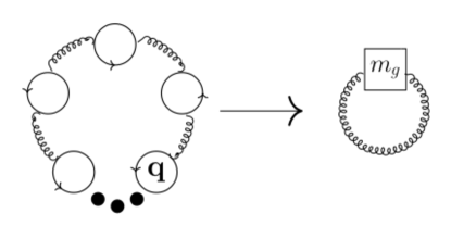
Figure 1: Connection between Ring sum and one-loop HTL.

A well-known important feature is that the all-loop summation gets rid of initially IR divergences, a mechanism related to the dynamical gluon screening mass. At $T=0,\mu\neq 0$, $m_{E}$ is obtained from the sole quark-loop contribution to the self-energy:

$$m^{2}_{E}=2\frac{\alpha_{s}}{\pi}\sum_{f}\mu_{f}^{2}=2\frac{\alpha_{s}}{\pi}N_{f}\mu^{2}.$$ (2)

Accordingly, in a rough picture, the all-loop soft mode summation can be essentially obtained from a one-loop calculation, within an alternative framework with a massive gluon (the graph on the right in Fig. 1), giving a contribution $P\sim m_{E}^{4}\ln m_{E}\sim\mu^{4}\alpha_{s}^{2}\ln\alpha_{s}$. This picture is rigorously embedded in the HTL formalismHTLbasic ; HTLptDense3L , that essentially provides a gauge invariant effective field theory (EFT) consistently including all HTL contributions with dressed momentum-dependent self-energies and vertices, and involving the screening gluon mass. The $\alpha_{s}^{3}$ last contribution in Eq.(1) was calculatedGorda:2018gpy ; Gorda:2021kme from HTL graphs with only gluons, NLO corrections to the right graph in Fig.1. The $m_{E}^{4}\alpha_{s}\ln^{2}(m_{E})\sim\alpha_{s}^{3}\ln^{2}\alpha_{s}$ was first obtained in Gorda:2018gpy , and recently the remnant soft terms were completed, obtainingGorda:2021kme ; Gorda:2021znl :

$$P^{\rm soft}_{\alpha_{s}^{3}}=\frac{N_{c}d_{A}\alpha_{s}m^{4}_{E}}{(8\pi)^{2}}\left(\frac{p_{-2}}{4\epsilon^{2}}+\frac{p_{-1}-2p_{-2}\ln\frac{m_{E}}{M_{s}}}{2\epsilon}\right.$$

$$\left.+2p_{-2}\ln^{2}\frac{m_{E}}{M_{s}}-2p_{-1}\ln\frac{m_{E}}{M_{s}}+p_{0}\right),$$ (3)

$$p_{-2}=\frac{11}{6\pi},\;\;p_{-1}\simeq 1.50731(19),\;\;p_{0}\simeq 2.2125(9).$$ (4)

All the $\mu$-dependence arises solely from the screening electrostatic mass, $m_{E}$ from Eq.(2). Notice in Eqs.(1)(3), besides $M_{h}$, the different scale $M_{s}$ introduced in Gorda:2021znl , for the soft sector. As explained in Gorda:2021kme ; Gorda:2021znl the presently unknown $\alpha_{s}^{3}$ hard (and mixed soft-hard) contributions are expected to cancel the remnant UV divergences and soft $\ln^{p}(m_{E}/M_{s})$ in (3), to let only $\ln^{p}\alpha_{s}$ and $\ln^{p}(M_{h}/\mu)$ terms ($p=1,2$). In absence of such explicit cancellations, since the soft terms can be treated as a separate $m_{E}$-dependent sector, to avoid large logarithms it appears sensible to chooseGorda:2021znl $M_{h}\sim{\cal O}(\mu)$ and $M_{s}\sim{\cal O}(m_{E})$.

HTL one-loop pressure: Our starting expression is the one-loop HTL pressure, calculable from the graph in Fig.1. In the present cold quark matter context it is evaluated at $T=0$, with (yet unspecified) mass $m_{g}$, obtaining

$$P_{\rm LO}^{\rm HTL}=\frac{d_{A}\ m_{g}^{4}}{(8\pi)^{2}}\left[\frac{1}{2\epsilon}+C_{11}-L+\epsilon\left(L^{2}+C_{21}L+C_{22}\right)\right]$$

$$\equiv m_{g}^{4}\left[-\frac{a_{1,0}}{2\epsilon}+a_{1,0}L+a_{1,1}+{\cal O}(\epsilon)\right]$$ (5)

where $L=\ln(\frac{m_{g}}{M})$ and $M$ is an arbitrary $\overline{\rm MS}$ scale. In Eq.(All order resummed leading and next-to-leading soft modes of dense QCD pressure) we also introduced a convenient notation for later purpose. The coefficient $C_{11}\sim 1.17201$ was first obtained in HTLptT0 . As explicited below, however, to work out complete NLL expressions we also need the ${\cal O}(\epsilon)$ terms, not previously available to our knowledge, that we have evaluated. We obtain $C_{21}=-2C_{11},C_{22}\simeq 2.16753$ (details can be found in suppmat ).
RG resummation: We consider the renormalization group (RG) operator (see e.g. Collins ), that parametrizes the scale variation in a (massive) theory:

$$M\frac{d}{dM}\equiv M\frac{\partial}{\partial M}+\beta(g^{2})\frac{\partial}{\partial g^{2}}-\gamma^{g}_{m}(g^{2})m_{g}\frac{\partial}{\partial m_{g}}\,,$$ (6)

where $M$ is a renormalization scale, $\beta(g^{2})\equiv\mbox{d}g^{2}/\mbox{d}\ln M$ dictates the running coupling, and the anomalous mass dimension $\gamma^{g}_{m}(g^{2})\equiv\mbox{d}(\ln m_{g})/\mbox{d}\ln M$ is further discussed below. In our convention with $g^{2}\equiv 4\pi\alpha_{s}$,

$$\beta(g^{2})=-2b_{0}^{g}g^{4}-2b_{1}^{g}g^{6}+\cdots,\;\gamma^{g}_{m}(g^{2})=\gamma^{g}_{0}g^{2}+\gamma^{g}_{1}g^{4}+\cdots$$ (7)

where $b_{0}^{g},b_{1}^{g}$ are the QCD pure gauge contributions

$$(4\pi)^{2}\,b_{0}^{g}=\frac{11N_{c}}{3},\;(4\pi)^{4}\,b_{1}^{g}=\frac{34N_{c}^{2}}{3}.$$ (8)

Given that HTL involves a gluon mass term $m_{g}$, from a RG standpointrgopt_phi4 we consider $m_{g}$ blind to its precise dynamical origin as a screening mass, motivating to use the massive RG Eq.(6). Indeed, despite the nonlocal HTL Lagrangian, the NNLO perturbative HTL calculations give new $m_{g}$-dependent UV divergences and related counterterms having a renormalizable form, as will be seen below, thus defining EFT anomalous dimensions in standard fashion. It is important to stress that the RG coefficients for such a massive theory are $T=0$ entities by definitions, even though they enter thermal or in-medium contributions as well. More precisely, within $T\neq 0$ HTL calculations, the divergences from $m_{g}\neq 0$ occur in two-loop order $\alpha_{s}(m^{2}_{g}T^{2},m^{3}_{g}T)$ terms, and the corresponding (unique) one-loop counterterm $\Delta m_{g}$ was obtained first in HTLpt2g . Using this $\Delta m_{g}$ and the standard relation between bare mass $m_{g}^{B}$, $Z_{m_{g}}$ counterterm and Eq.(7): $m^{B}_{g}\equiv m_{g}\,Z_{m_{g}}\simeq m_{g}(1-g^{2}\,\gamma_{0}^{g}/(2\epsilon)+{\cal O}(g^{4}))$, we easily identify:

$$\gamma^{g}_{0}=\frac{11N_{c}}{3(4\pi)^{2}}\equiv b_{0}^{g}.$$ (9)

Namely, the LO interactions from HTL that contribute to renormalize $m_{g}$ give a divergent contribution identical to the one defining $b_{0}^{g}$. Although striking, this equality of pure gauge $b_{0}^{g}$ and $\gamma_{0}^{g}$ is merely a one-loop order accident. Incidentally, it is worth noting that the same result (9) was obtained independently from a localizable, renormalizable gauge-invariant setup for a (vacuum) gluon massmgvac : this is not a coincidence since those universal RG quantities are vacuum quantities independent of $T,\mu$. The two-loop order $\gamma_{1}^{g}$, entering the NLO RG Eq.(7) in our construction, has also been calculated from the same $T=\mu=0$ formalism, with the resultmgvac2 $(4\pi)^{4}\gamma_{1}^{g}=77N_{c}^{2}/12$. Furthermore, the mass renormalization within Eq.(All order resummed leading and next-to-leading soft modes of dense QCD pressure), $P_{\rm LO}^{\rm HTL}(m_{g}\to m_{g}Z_{m_{g}})$, generates additional terms that combine with genuine two-loop contributions Eq.(3). Importantly, the unwanted nonlocal $\ln(m_{E}/M_{s})/\epsilon$ divergence in Eq.(3) exactly cancels in those combinations, while (local) remnant divergences after mass renormalization are renormalized by vacuum energy ${\cal E}_{0}$ ($\equiv-P$) counterterms, always necessary in a massive theory. According to Weinberg’s theoremCollins , such local counterterms prove the renormalizability of the $T=0$ HTL pressure at NLO $\alpha_{s}m_{g}^{4}$, i.e. NNNLO $\alpha_{s}^{3}$. The LO vacuum energy counterterm is the one determined in HTLHTLpt2g ; HTLptT0 , $\Delta{\cal E}_{0}^{(1)}=d_{A}m_{g}^{4}/(8\pi)^{2}/(2\epsilon)$. At NLO its expression is given in suppmat . Remark that renormalizing $m_{g}$ in Eq.(All order resummed leading and next-to-leading soft modes of dense QCD pressure) also modifies the finite coefficients in Eq.(4), as

$$2p_{-2}\rightarrow\!p_{-2},\;p_{-1}\to\!p_{-1}-\frac{8\pi\gamma_{0}^{g}}{N_{c}}(C_{11}-\!\frac{1}{4})\simeq p_{-1}\!\!-0.5381,$$

$$p_{0}\to p_{0}-\frac{8\pi\gamma_{0}^{g}}{N_{c}}(C_{22}-\frac{C_{11}}{2})\simeq p_{0}-0.9229.$$ (10)

In Gorda:2021kme nontrivial cancellation mechanisms between soft $\alpha_{s}m_{E}^{4}$ and (presently not known) $\alpha_{s}^{3}$ hard contributions are convincingly argued to remove the divergent terms in Eq.(3), and to obtain the correct $\alpha_{s}^{3}\ln^{2}m_{E}$ coefficient, $2p_{-2}\to p_{-2}$. In our massive renormalized scheme the right $p_{-2}$ originates directly from standard mass renormalization cancellation mechanisms. This simple alternative picture appears consistent with generic EFT constructionsEFTrev , where all EFT UV divergences are renormalized, defining EFT anomalous dimensions, sufficient to extract $\ln m_{E}$ dependencies from the RG.
Having identified these key RG ingredients at $T=0$, obtaining the LL and NLL at successive orders follows a well-established procedureCollins . Power countingGorda:2021kme dictates the soft pressure expansion to all orders

$$P^{soft}\sim m^{4}_{g}\sum_{p=1}^{\infty}\left(g^{2}\right)^{p-1}\>\sum_{l=0}^{p}a_{p,l}\ln^{p-l}(\frac{m_{g}}{M})$$ (11)

with $M$ the ($\overline{\rm MS}$ scheme) renormalization scale. The $a_{p,0}\ln^{p}(m_{g}/M),p\geq 1$ are the leading logarithmic (LL), $a_{p,1}\ln^{p-1}(m_{g}/M),p\geq 2$ the next-to-leading logarithmic (NLL) coefficients and so on, with $a_{p,p}$ the non-logarithmic coefficients at successive orders. Upon applying the RG Eq.(6) on Eq.(11) considering $g$ fixed, we obtain recurrence relations. First for the LL series

$$-p\>a_{p,0}=[4\gamma_{0}^{g}+2b_{0}^{g}(p-2)]a_{p-1,0},\;\;p\geq 2$$ (12)

where $a_{1,0}$ is given in Eq.(All order resummed leading and next-to-leading soft modes of dense QCD pressure). Before proceeding it is worth to give a first concrete outcome of Eq.(12), that immediately gives at NLO:

$$a_{2,0}=-2\gamma_{0}^{g}a_{1,0}\equiv-2b_{0}^{g}a_{1,0}$$ (13)

determining the LL term: $g^{2}\,m_{g}^{4}\,a_{2,0}\ln^{2}(m_{g}/M)$, that upon using Eqs.(All order resummed leading and next-to-leading soft modes of dense QCD pressure),(8) gives $(4\pi)a_{2,0}=N_{c}d_{A}/(8\pi)^{2}\,p_{-2}$, that perfectly matches Eqs.(3),(4) for $m_{g}\equiv m_{E}$ with $p_{-2}$ in (10). We stress that all LL in Eq.(12) rely on the sole one-loop $\ln(m_{g}/M)$ coefficient $a_{1,0}$ in Eq.(All order resummed leading and next-to-leading soft modes of dense QCD pressure), thus are completely independent from the results in Gorda:2018gpy ; Gorda:2021kme , where $m_{E}^{4}\alpha_{s}\ln^{2}m_{E}$ was obtained from involved two-loop HTL calculations. The important feature to obtain it from the above simple RG relations is having identified $\gamma_{0}^{g}$. More interestingly, Eq.(12) gives all higher order LL coefficients, a new result that we resum explicitly below.
One obtains similarly the NLL series (defined for $p\geq 2$)

$$(1-p)a_{p,1}=[4\gamma_{0}^{g}+2b_{0}^{g}(p-2)]a_{p-1,1}$$

$$+[4\gamma_{1}^{g}+2b_{1}^{g}(p-3)]a_{p-2,0}+\gamma_{0}^{g}(p-1)a_{p-1,0}.\;\;$$ (14)

We recall that at a given perturbative order $g^{2p}$, the only new terms to calculate are the single logarithm $a_{p,p-1}$ and nonlogarithmic $a_{p,p}$ terms. Both LL and NLL series above are convergent and can thus be resummed.
Perturbatively RG invariant pressure: Before giving resummed LL and NLL expressions, it is convenient to develop a related important ingredient of our construction, namely to restore a RG invariant (RGI) massive pressure. Indeed, applying Eq.(6) to Eq.(All order resummed leading and next-to-leading soft modes of dense QCD pressure) gives a remnant scale dependence at leading HTL order, $\sim m_{g}^{4}\ln M$, a well-known feature of massive theories. The appropriate way to deal with this is to realize that the RG Eq.(6) has an inhomogeneous term, defining a (gluon) vacuum energy anomalous dimension $\hat{\Gamma}_{0}^{g}(g^{2})=\Gamma_{0}^{g}+\Gamma_{1}^{g}g^{2}+\cdots$, by analogy with other massive sector vacuum energiesE0anomdim ; E0phi4 :

$$\frac{d\,P^{\rm HTL}}{d\ln M}\equiv-m_{g}^{4}\hat{\Gamma}_{0}^{g}(g^{2})=\frac{d}{d\ln M}(m_{g}^{4}\sum_{k\geq 0}s_{k}^{g}g^{2k-2}),$$ (15)

$\hat{\Gamma}_{0}^{g}(g^{2})$ being related to the vacuum energy counterterms (see suppmat ). Thus an RGI combination is $P_{RGI}\equiv P^{\rm HTL}-m_{g}^{4}\sum_{k}s_{k}g^{2k-2}$, where the $s_{k}^{g}$ coefficients are most simply determinedrgopt_phi4 perturbatively from the second equality in Eq.(15): at LO and NLO we obtain respectively

$$s_{0}^{g}=-\frac{a_{1,0}}{2(b_{0}^{g}-2\gamma_{0}^{g})}=\frac{-d_{A}}{2(8\pi)^{2}\,b_{0}^{g}},$$ (16)

$$s_{1}^{g}=a_{1,1}+\frac{a_{2,1}}{4\gamma_{0}^{g}}+\frac{a_{1,0}}{4}+\frac{s_{0}^{g}}{2\gamma_{0}^{g}}(b_{1}^{g}-2\gamma_{1}^{g}),$$ (17)

where $a_{1,1}=-a_{1,0}C_{11}$ in Eq.(All order resummed leading and next-to-leading soft modes of dense QCD pressure). Embedding Eq.(16) within Eq.(12) one can easily resum the LL series as

$$P^{\rm sum}_{\rm LL}=-\frac{s_{0}^{g}\>m_{g}^{4}}{g^{2}}f_{1}^{1-4(\frac{\gamma_{0}^{g}}{2b_{0}^{g}})}=-\frac{s_{0}^{g}\>m_{g}^{4}}{g^{2}}f_{1}^{-1},$$

$$f_{1}=1+2b_{0}^{g}\,g^{2}\ln\frac{m_{g}}{M},$$ (18)

where we also used Eq.(9). It is straightforward to check that Eq.(18) reproduces at all orders the coefficients in Eq.(12). The last equality in Eq.(18) tells that the LL series iterates simply like the (pure gauge) running coupling, but this is merely an accident of LO RG Eq.(9).
Similarly, after more algebra one can resum formally the NLL series. Adapting results fromjlrgsum we obtain:

$$P^{\rm sum}_{\rm NLL}=\frac{-s_{0}^{g}\,m_{g}^{4}}{g^{2}\,f_{2}^{4A_{0}-1}}[R(f_{2})]^{B}(1-\frac{a^{\prime}_{1,1}\,g^{2}}{s_{0}^{g}\,f_{2}}-\frac{a_{2,2}\,g^{4}}{s_{0}^{g}\,f_{2}^{2}}),$$ (19)

$$R(f_{2})=(1+g^{2}\,b_{1}^{g}/(b_{0}^{g}f_{2}))/(1+g^{2}\,b_{1}^{g}/b_{0}^{g}),$$

$$\!\!\!f_{2}=1+\left[2b_{0}^{g}\,g^{2}+2(b_{1}^{g}-\gamma_{0}^{g}b_{0}^{g})g^{4}\right]\ln\frac{m_{g}}{M}+{\cal O}(g^{6}),$$ (20)

and $A_{0}=\gamma_{0}^{g}/(2b_{0}^{g}),A_{1}=\gamma_{1}^{g}/(2b_{1}^{g}),B=4(A_{1}-A_{0})$. The exact $f_{2}$ expression, reproducing Eq.(14) to all orders from Eq.(19), is given in suppmat . Eq.(20) gives numerically good approximations as long as the coupling is not too large ($\alpha_{s}\lesssim 0.5$).
A few remarks are worth regarding the input content of Eq.(19): i) It is rather generic, but numerically relies on the lowest order purely soft NLL coefficient $a_{2,1}\propto p_{-1}$ in Eq.(3), calculated in Gorda:2021kme . Accordingly, Eq.(19) does not include the (presently unknown) QCD mixed soft-hard NLL contributions, see Gorda:2021kme . ii) One obtains $a^{\prime}_{1,1}\equiv a_{1,1}-s_{1}^{g}$ with $a_{1,1}$ defined in Eq.(All order resummed leading and next-to-leading soft modes of dense QCD pressure), since the NLO subtraction coefficient $s_{1}^{g}$ in Eq.(17) contributes a correction to $a_{1,1}$. iii) $a_{2,2}$ in Eq.(19) incorporates the ${\cal O}(g^{2}m_{g}^{4})$ non-logarithmic term $p_{0}$ in Eq.(3): the precise connection between the parameters in Eq.(19) and $p_{-1},p_{0}$ in Eqs.(3),(10) is $a_{2,1}=N_{c}/(4\pi)a_{1,0}(2p_{-1})$, $a_{2,2}=-N_{c}/(4\pi)a_{1,0}\,p_{0}$, after modifying $p_{-1},p_{0}$ in Eq.(10).
Soft and hard pressure matching: The massive RG construction above basically concerns the soft pressure contributions, thus $\ln m_{g}/M\to\ln m_{E}/M_{s}$, with overall factor $m_{E}^{4}\sim\alpha_{s}^{2}$, see Eq.(2). While the hard contribution in Eq.(1), known exactly only at $\alpha_{s}^{2}$-order, is added perturbatively to Eqs.(18),(19). The latter RGI expressions formally cancel the soft scale dependence up to neglected ${\cal O}(g^{2}m_{E}^{4})$, ${\cal O}(g^{4}m_{E}^{4})$ terms respectively. At ${\cal O}(\alpha_{s}^{2})$, it is equivalent to the complete soft scale cancellation operating in the factorization picture, thus, we can choose any $M_{s}$. While at $\alpha_{s}^{p\geq 3}$-orders, partial ignorance of hard and mixed contributions incites to take $M_{s}\sim{\cal O}(m_{E})$ in the $\ln m_{E}/M_{s}$ terms.
Another feature to account while combining the soft and hard contributions is that Eq.(19) entails a nonlogarithmic term $\sim\alpha_{s}^{2}a_{1,1}$ with $a_{1,1}$ from Eq.(17), obviously different from the genuine “soft +hard” $\alpha_{s}^{2}$ term in Eq.(1). Since only soft contributions are RG-resummed, to avoid wrong contaminations in nonlogarithmic hard terms from RG-induced NLL soft terms, one should perturbatively subtract $a_{1,1}m_{E}^{4}$ from the total expression (which does not affect higher order NLL terms generated by $a_{1,1}$ within Eq.(19)).
As a last important subtlety, note that although the subtraction terms as above determined, Eqs.(16),(17), are sufficient to define LO and NLO RGI pressures Eqs.(18),(19), actually the complete integration of Eq.(15) entails an extra boundary condition (see suppmat ):

$$P^{\rm BC}_{\rm RGI}=m_{g}^{4}(M_{0})(\frac{s_{0}^{g}}{g^{2}(M_{0})}+s_{1}^{g}),$$ (21)

of similar form as the subtraction terms but involving a (boundary) scale $M_{0}\neq M$. We can use this freedom to set $M_{0}$ such that Eq.(21) provides an appropriate EFT-matchingEFTrev of the soft pressure to the full one at ${\cal O}(\alpha_{s}^{2})$, i.e. with $M_{0}\sim{\cal O}(\mu)$, consistently also with the Stefan-Boltzmann limit.
Collecting all, our final pressure expression is obtained upon formally replacing $P^{\rm soft}_{\alpha_{s}^{3}}$ in Eq.(1) by

$$P^{\rm sum}_{\alpha_{s}^{p\geq 3}}=P^{\rm sum}_{\rm(N)LL}+P^{\rm BC}_{\rm RGI}-m_{E}^{4}(a_{1,1}+a_{1,0}\ln\frac{m_{E}}{M_{s}})-P^{\rm match}_{\alpha_{s}^{2}}$$ (22)

with $a_{1,1}=0$, $s_{1}^{g}\equiv 0$ for $P^{\rm sum}_{\rm LL}$, and $P^{\rm match}_{\alpha_{s}^{2}}$ given in Eq.(B10) in suppmat . The last three terms in Eq.(22) are required to match Eq.(1) consistently (i.e. without double counting), so that all RG-induced extra terms are ${\cal O}(\alpha_{s}^{3})$.

Numerical results and comparisons: In Fig.2 the RGI LL and NLL resummed pressures from Eq.(22) are compared to the present state-of-the-art Eqs.(1),(3) as function of $\mu_{B}=3\mu$. The central scale values $M_{h}=2\mu$ and the $\mu\leq M_{h}\leq 4\mu$ remnant scale dependence are illustrated for the different quantities, using in Eqs.(1),(22) the exact NLO QCD running coupling $\alpha_{s}(M_{h})$ withPDG2018 $\Lambda_{\overline{\rm MS}}\sim 0.32$ GeV. For sensible comparisons we also adopt the minimal sensitivity-determinedpms soft scale in Gorda:2021znl , $M_{s}\sim 0.275m_{E}$. Finally, we fix $M_{0}=2\mu$ in Eq.(21), a natural choice as it calibrates Eq.(22) to the central $M_{h}$ values of the NNLO pressure.
Note first importantly that the sole LL resummation, given by Eq.(18) with $-s_{0}^{g}\to a_{1,0}g^{2}\ln m_{g}/M$, gives a sizeably reduced scale dependence, compared to the NNLO pressure Eq.(1) at ${\cal O}(\alpha_{s}^{2})$, as Eq.(18) induces positive $\alpha_{s}^{p\geq 3}$ contributions partly cancelling the negative $\alpha_{s}^{2}$ coefficient in Eq.(1). However, this effect is approximately cancelled once including $p_{-1},p_{0}$ $\alpha_{s}^{3}$-order terms Eqs.(4),(10). Next, for the LL and NLL RGI pressures, deviations from the state-of-the-art (“NNLO + soft $\rm N^{3}LO$” in Fig.2) are noticeable. The central scale ($M_{h}=2\mu$) RGI pressure is slightly higher for fixed $\mu$ values, with very moderate differences between LL and NLL pressures. Importantly, the remnant scale dependencies of the resummed pressures are reduced as compared to NNLO + soft $\rm N^{3}LO$ results: only slightly for the LL pressure, due to cancellations with $p_{-1},p_{0}$ ${\cal O}(\alpha_{s}^{3})$ terms, but significantly for the NLL one, both for $M_{h}$ and $M_{s}$ variations, due to $\alpha_{s}^{p\geq 3}$ terms induced both by NLL and the RGI-restoring terms in Eqs.(19),(22).

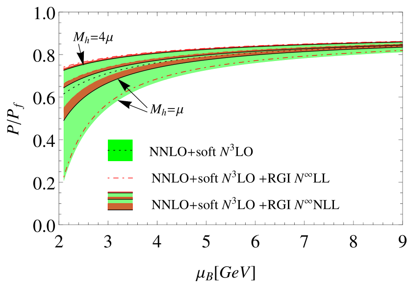
Figure 2: NNLO + soft $\rm N^{3}LO$ Eqs.(1),(3) versus NNLO + soft $\rm N^{3}LO$ +RGI LL, NLL resummed pressures, as function of $\mu_{B}=3\mu$, with $\mu\leq M_{h}\leq 4\mu,M_{s}\simeq 0.275m_{E}$, $M_{0}=2\mu$. For the RGI NLL resummed pressure, $M_{s}$ variations within $[M_{s}/2,2M_{s}]$ are shown in addition as darker bands.

In conclusion, we have obtained compact explicit expressions for the all order “double” resummations of LL and NLL soft contributions to the cold and dense QCD pressure, that goes well beyond previously established results. Our RG resummation construction moreover gives clearly improved residual scale dependence. This should provide improved control towards lower $\mu_{B}$ values to match with the extrapolated EoS from the nuclear matter density region. We thus anticipate that our present results may have strong implications once embedded within a more realistic EoS. It is not difficult to extend our framework to include different chemical potential and nonzero masses for the quarks, in order to more realistically describe the EoS relevant for beta equilibrium and neutron star properties, that we leave for future investigation.

Acknowledgments: We thank Marcus B. Pinto and Aleksi Vuorinen for discussions.

Appendix A One-loop $T=0$ HTL pressure calculation

We give here the main steps of our derivation of Eq.(All order resummed leading and next-to-leading soft modes of dense QCD pressure), where the ${\cal O}(\epsilon)$ contributions is a new result, to the best of our knowledge. For the HTL formalism and relevant expressions of the gluon propagator and self-energies we refer e.g. to HTLpt2g ; HTLrev2020 . We mainly follow the convenient Euclidean $T=0$ conventions and expressions in Gorda:2021kme , to which we refer for more details here skipped. The one-loop graph in the right of Fig.1 gives for the HTL free energy (see e.g. HTLpt2g ; HTLptT0 ):

$$\Omega^{\rm HTL}_{\rm LO}=-\frac{d_{A}}{2}\int_{K}\left((d-1)\ln[\Delta_{T}(K)]+\ln[\Delta_{L}(K)]\right),$$ (23)

where $K^{\mu}=(K_{0},{\bf k})$ is an Euclidean vector in $d+1$ dimensions (the integration measure in (23) will be specified below),

$$\Delta_{T,L}(K)\equiv\frac{1}{K^{2}+\Pi_{T,L}(K)},$$ (24)

$\Pi_{T,L}$ being the transverse and longitudinal components of the one-loop HTL self-energy tensor

$$\Pi^{\mu\nu}(K)=T^{\mu\nu}(\hat{K})\Pi_{T}(K)+L^{\mu\nu}(\hat{K})\Pi_{L}(K),$$ (25)

where the $T,L$ projection operators are

$$T^{\mu\nu}(\hat{K}) \equiv\delta^{\mu i}\delta^{\nu j}\left(\delta^{ij}-\hat{k}^{i}\hat{k}^{j}\right)$$ (26)

$$L^{\mu\nu}(\hat{K}) \equiv\delta^{\mu\nu}-\hat{K}^{\mu}\hat{K}^{\nu}-T^{\mu\nu}(\hat{K})$$

with $\hat{K}=K/|K|$ and $\hat{\bf k}=\bf k/|\bf k|$.
For the HTL approximation relevant for cold quark matter, one has

$$\Pi^{\mu\nu}(K)=m_{g}^{2}\int_{\hat{\mathbf{v}}}\left(\delta^{\mu 0}\delta^{\nu 0}-\frac{iK_{0}}{K\cdot V}V^{\mu}V^{\nu}\right)$$ (27)

where $V^{\mu}\equiv(-i,\hat{\mathbf{v}})$ is a lightlike vector, with $\hat{\mathbf{v}}$ a $d$-dimensional unit vector. Taking the trace and $00$ components of Eq.(25), and Eq.(27) with appropriate $d$-dimensional measures, leads to

$$\Pi^{\mu\mu}(K)=m_{g}^{2}\int_{\hat{\mathbf{v}}}\delta^{00}=m_{g}^{2}$$ (28)

$$\Pi^{00}(K)=m_{g}^{2}\left[1+\int_{\hat{\mathbf{v}}}\frac{iK_{0}}{-iK_{0}+|{\mathbf{k}}|z_{v}}\right]$$

$$=m_{g}^{2}\left[1-_{2}\!{F}_{1}\left(\frac{1}{2},1,\frac{d}{2};-\frac{{\mathbf{k}}^{2}}{K_{0}^{2}}\right)\right],$$ (29)

where ${}_{2}\!\,{F}_{1}$ is the hypergeometric function. From Eq.(29) it is not difficult to derive the Taylor expansion in $\epsilon$ of $\Pi^{00}$, thus of $\Pi_{L},\Pi_{T}$ from successive derivatives $\partial_{c}\,[_{2}\!{F}_{1}(a,b,c;z)]$. Finally, expressing $\Pi_{L,T}$ in terms of the Euclidean $\phi_{K}$ angle, $\tan\phi_{K}\equiv|{\bf k}|/K_{0}$, gives

$$\Pi_{T}(\phi_{K})=\frac{m_{g}^{2}}{2}\cot(\phi_{K})\left[\bar{\phi}_{K}\csc^{2}(\phi_{K})-\cot(\phi_{K})\right]+{\cal O}(\epsilon)$$

$$\Pi_{L}(\phi_{k})=m_{g}^{2}\csc^{2}(\phi_{K})\left[1-\bar{\phi}_{K}\cot(\phi_{K})\right]+{\cal O}(\epsilon),$$ (30)

where $\bar{\phi}_{K}\equiv\arctan[\tan(\phi_{K})]$, and similarly for higher order terms in $\epsilon$. From such expressions we can evaluate Eq.(23), with $\int_{K}\equiv 2\pi^{d/2}/\Gamma(d/2)/(2\pi)^{(d+1)}\int_{0}^{\pi}d\phi_{k}\sin^{d-1}(\phi_{k})\times\int_{0}^{\infty}dk\,k^{d}$. The integral over $k\equiv|K|$ is easily performed analytically, with the leading UV-divergent term $\sim 1/\epsilon$ extracted. To obtain next the finite and ${\cal O}(\epsilon)$ coefficients requires to expand $\Pi_{L,T}$ up to order $\epsilon^{2}$ in Eq.(30). Upon numerical remnant angular integration we obtain after algebra the $T=0$ pressure $P_{\rm LO}^{\rm HTL}=-\Omega_{\rm LO}^{\rm HTL}$ in the $\overline{\rm MS}$-scheme:

$$P_{\rm LO}^{\rm HTL}=-(\frac{e^{\gamma_{E}}M^{2}}{4\pi})^{\epsilon}\,\frac{d_{A}}{2-\epsilon}\,\sec(\pi\frac{d}{2})\frac{2\pi^{\frac{d}{2}}}{\Gamma(\frac{d}{2})}$$

$$\times(\frac{m_{g}}{2\pi})^{d+1}(\frac{\pi^{2}}{16})\left(1+d_{11}\epsilon+d_{12}\epsilon^{2}\right)$$ (31)

where $M$ is the $\overline{\rm MS}$ arbitrary scale and

$$d_{11}\simeq 1.23032,\;d_{12}\simeq 1.04214,$$ (32)

that upon expanding Eq.(31) in $\epsilon$ with $d=3-2\epsilon$ gives Eq.(All order resummed leading and next-to-leading soft modes of dense QCD pressure) with

$$C_{11}=-\frac{1}{2}C_{21}=\frac{5}{4}-\ln 2+\frac{d_{11}}{2}\simeq 1.17201,$$

$$C_{22}=(\frac{5}{4}-\ln 2)d_{11}+\frac{d_{12}}{2}+\ln^{2}2-\frac{5}{2}\ln 2+\frac{21}{8}-\frac{\pi^{2}}{24}\simeq 2.16753,$$ (33)

where $C_{11}$ was first obtained in HTLptT0 .

Appendix B Vacuum energy anomalous dimension and RG-invariant pressure

Once combining the genuine two-loop contributions Eq.(3) and Eq.(31) with renormalized mass, $P_{\rm LO}^{\rm HTL}(m_{g}\to m_{g}Z_{m_{g}})$ where $Z_{m_{g}}\simeq(1-g^{2}\,\gamma_{0}^{g}/(2\epsilon)+{\cal O}(g^{4}))$ in our normalization, the $\ln(m_{E})/\epsilon$ in Eq.(3) cancels, and remnant local divergences are renormalized by minimal subtraction, defining the NLO vacuum energy counterterm:

$$\Delta{\cal E}_{0}^{(2)}=\frac{d_{A}\,m_{g}^{4}}{(8\pi)^{2}}\left\{\frac{1}{2\epsilon}+N_{c}(\frac{g^{2}}{4\pi})\left(-\frac{11}{24\pi\,\epsilon^{2}}+[\frac{p_{-1}}{2\epsilon}-\frac{11}{6\pi\epsilon}(C_{11}-\frac{1}{4})]\right)\right\}\equiv Z_{0}^{g}(g^{2})m_{g}^{4},$$ (34)

where the LO term was derived in standard HTLHTLpt2g . As remarked in the main text, the resulting finite pressure is not RG invariant: rather, Eq.(34) implies a gluon vacuum energy density anomalous dimension $\hat{\Gamma}_{0}^{g}(g^{2})$, modifying the homogeneous RG equation as:

$$\frac{d\,{\cal E}_{0}}{d\ln M}[=-\frac{d\,P^{\rm HTL}}{d\ln M}]\equiv\hat{\Gamma}_{0}^{g}(g^{2})m^{4}_{g},$$ (35)

where $\hat{\Gamma}_{0}^{g}(g^{2})=\Gamma_{0}^{g}+\Gamma_{1}^{g}g^{2}+\cdots$. In other words, the massive pressure (equivalently vacuum energy), considered as a dimension four EFT operator, starts to mix with the unit operator $\sim m_{g}^{4}\mathds{1}$ already at one-loop. $\hat{\Gamma}_{0}^{g}(g^{2})$ can be obtained from the counterterm Eq.(34): we define (see e.g. E0anomdim )

$${\cal E}_{0}^{B}\equiv M^{-2\epsilon}\left({\cal E}_{0}(g^{2})-m_{g}^{4}\,Z_{0}^{g}(g^{2})\right)$$ (36)

with ${\cal E}_{0}^{B},{\cal E}_{0}$ the bare and renormalized vacuum energies respectively and $Z_{0}^{g}$ the (dimensionless) counterterm in Eq.(34). Then applying the RG equation (6): $d({\cal E}_{0}^{B})/d\ln M\equiv 0$ (with $\beta(g^{2})\to\overline{\beta}(g^{2})\equiv-2\epsilon g^{2}+\beta(g^{2})$ as it is appropriate for bare quantities), we obtain after straightforward algebra

$$\hat{\Gamma}_{0}^{g}(g^{2})=(-4\gamma_{m}(g^{2})-2\epsilon)Z_{0}^{g}(g^{2})+\overline{\beta}(g^{2})\frac{\partial}{\partial g^{2}}Z_{0}^{g}(g^{2}).$$ (37)

Up to NLO this gives

$$\Gamma_{0}^{g}=a_{10}=-\frac{d_{A}}{(8\pi)^{2}},\;\;\Gamma_{1}^{g}=2a_{10}\left(\frac{N_{c}}{4\pi}\right)\left(p_{-1}-\frac{11}{3\pi}(C_{11}-\frac{1}{4})\right).$$ (38)

Next we consider the complete integral solution of the RG Eq.(35), formally obtained as (see e.g. Collins )

$$P^{\rm HTL}(g^{2}(M),m(M))=P^{\rm HTL}(g^{2}(M_{0}),m(M_{0}))+\int_{g^{2}(M_{0})}^{g^{2}(M)}dx\left\{\frac{-\hat{\Gamma}_{0}^{g}(x)}{\beta(x)}\exp\left[-4\int_{g^{2}(M_{0})}^{x}dy\frac{\gamma_{m}(y)}{\beta(y)}\right]\right\}m^{4}_{g}(M_{0}),$$ (39)

where $M_{0}$ is a reference or “initial” scale. Working out Eq.(39) explicitly at perturbative NLO, using $\beta(g^{2})$, $\gamma_{m}(g^{2})$ from Eq.(7), we obtain after some algebra the (NLO) RG-invariant combination

$$P^{\rm HTL}_{RGI}\equiv P^{\rm HTL}-\left[m_{g}^{4}(M)\left(\frac{s_{0}^{g}}{g^{2}(M)}+s_{1}^{g}\right)-m_{g}^{4}(M_{0})\left(\frac{s_{0}^{g}}{g^{2}(M_{0})}+s_{1}^{g}\right)+{\cal O}(m_{g}^{4}g^{2})\right].$$ (40)

Note that to obtain the final form of Eq.(40) we have identified the NLO running mass expression:

$$m_{g}(M)\simeq m_{g}(M_{0})\left(\frac{g^{2}(M)}{g^{2}(M_{0})}\right)^{\frac{\gamma_{0}^{g}}{2b_{0}^{g}}}\left[1+\frac{2}{(b_{0}^{g})^{2}}(b_{0}^{g}\gamma_{1}^{g}-b_{1}^{g}\gamma_{0}^{g})\,g^{2}(M_{0})+{\cal O}(g^{4})\right],$$ (41)

and used the relations between $s_{0}^{g},s_{1}^{g}$ in Eqs.(16),(17) and vacuum energy anomalous dimension coefficients $\Gamma_{i}^{g}$:

$$\Gamma_{0}^{g}=-2s_{0}^{g}(b_{0}^{g}-2\gamma_{0}^{g});\;\;\Gamma_{1}^{g}=4\gamma_{0}^{g}s_{1}^{g}-2s_{0}^{g}(b_{1}^{g}-2\gamma_{1}^{g}).$$ (42)

Note that all the terms $\propto m_{g}^{4}(M)$ in Eq.(40), sufficient for restoring RGI with respect to $M$, can be obtained in a more pedestrian way by working out perturbatively the second equality in Eq.(15), however missing the boundary terms $\propto m_{g}^{4}(M_{0})$ of the complete solution Eq.(40). For sufficiently large $M_{0}$, the latter boundary terms behave as $s_{0}^{g}[2b_{0}^{g}\ln(M_{0}/\Lambda_{\overline{\rm MS}})]^{1-4\gamma_{0}^{g}/(2b_{0}^{g})}\sim\ln^{-1}(M_{0}/\Lambda_{\overline{\rm MS}})$, where $\Lambda_{\overline{\rm MS}}$ is the basic QCD scale. The occurrence of $1/g^{2}$ terms in Eq.(40) is related to the LO $\hat{\Gamma}_{0}^{g}(g^{2})$ being ${\cal O}(1)$ in $g$, a consequence of the ${\cal O}(1)$ LO pressure $1/\epsilon$ divergence. However, the difference of the two terms in brackets in Eq.(40) has its leading perturbative contribution starting at ${\cal O}(g^{4})$, more precisely:

$$P^{extra}_{\alpha_{s}^{2}}=P_{f}(\frac{2N_{f}}{\pi^{2}})\alpha_{s}^{2}(M_{0})(\frac{b_{0}}{b_{0}^{g}})\ln\frac{M_{0}}{M}\equiv P^{match}_{\alpha_{s}^{2}},$$ (43)

where $b_{0}\equiv b_{0}^{g}-(2/3)N_{f}/(4\pi)^{2}$, i.e. $b_{0}/b_{0}^{g}=9/11$ for $N_{f}=3$, accounts for the full QCD running coupling used for the total (soft + hard) pressure. We thus subtract Eq.(43) in Eq.(22) to consistently match the NNLO pressure Eq.(1) up to higher order $\alpha_{s}^{p\geq 3}$ terms.
Collecting all relevant terms, a convenient compact expression for the total pressure with Eq.(22) restricted to LL terms reads explicitly:

$$P^{\rm sum,LL}_{\alpha_{s}^{p\geq 3}}=P^{cqm}_{\alpha_{s}^{2}}+P_{f}(\frac{2N_{f}}{\pi^{2}})\left(\frac{1}{8\pi\,b_{0}^{g}}\left[\frac{\alpha_{s}}{1+8\pi b_{0}^{g}\,\alpha_{s}\ln\frac{m_{E}}{M_{s}}}-\alpha_{s}(M_{0})\right]+\alpha_{s}^{2}\ln\frac{m_{E}}{M_{s}}-\alpha_{s}^{2}(M_{0})\frac{b_{0}}{b_{0}^{g}}\,\ln\frac{M_{0}}{M_{h}}\right),$$ (44)

with $P^{cqm}_{\alpha_{s}^{2}}$ given in Eq.(1), $b_{0}^{g}$ in Eq.(8), and $\alpha_{s}\equiv\alpha_{s}(M_{h})$.

Appendix C Compact NLL resummation

In this appendix we give some more details on the NLL resummation. Rather than working out the result Eq.(19) directly from Eq.(14) which is tedious, it is more convenient to equivalently first derive an exact NLO running mass expression $m_{R}(M^{\prime})=m_{R}(M)\exp(-\int^{g^{2}(M^{\prime})}_{g^{2}(M)}\gamma_{m}(g)/\beta(g))$ using Eq.(6), with the boundary conditionjlrgsum $m_{R}(m_{R})\equiv m_{R}$. Then, considering dimensionally dictated expression $\propto m_{R}^{4}$ appropriate to match a vacuum energy and adding nonlogarithmic perturbative contributions, it leads after some algebra to Eq.(19), with

$$f_{2}=1+2b_{0}^{g}\,g^{2}\left\{\ln\frac{m_{g}}{M}+(C-A_{0})\ln f_{2}\right.$$

$$\left.+(C+A_{1}-A_{0})\ln R(f_{2})\right\}$$

$$=1+\left[2b_{0}^{g}\,g^{2}+2(b_{1}^{g}-\gamma_{0}^{g}b_{0}^{g})g^{4}\right]\ln\frac{m_{g}}{M}+{\cal O}(g^{6}).$$ (45)

where $A_{0}=\gamma_{0}^{g}/(2b_{0}^{g})$, $A_{1}=\gamma_{1}^{g}/(2b_{1}^{g})$, $C=b_{1}^{g}/(2(b^{g}_{0})^{2})$ and $R(f_{2})$ is defined after Eqs.(19),(20). Notice that $f_{2}$ in Eq.(45) is an implicit function, that should be iterated to correctly reproduce (analytically) the NLL coefficients in Eq.(14) to all orders. More conveniently truncating it at order $g^{4}$, i.e. using the last line of Eq.(45), numerically gives a very good approximation as long as the coupling is not too large.

Next, we give an alternative exact compact expression of Eq.(19) in terms of explicitly RGI quantities, more convenient than the implicit relation in first line of Eq.(45). Defining the two-loop order RGI massjlrgsum

$$\hat{m}_{g}=2^{C}m_{g}(2b_{0}^{g}\,g^{2})^{-A_{0}}(1+b_{1}^{g}\,g^{2}/b_{0}^{g})^{A_{0}-A_{1}},$$ (46)

$F_{2}=f_{2}/(2b_{0}^{g}\,g^{2})$, and using the exact two-loop running coupling, implicit $g^{2}(M)$ solution of

$$\Lambda_{\overline{\rm MS}}=Me^{-1/(2b_{0}^{g}g^{2})}(b_{0}^{g}\,g^{2}/(1+b_{1}^{g}\,g^{2}/b_{0}^{g}))^{-C},$$ (47)

Eq.(19) with $m_{g}\to m_{E}$ can be rewritten

$$P^{\rm sum}_{NLL}=-2b_{0}^{g}s_{0}^{g}2^{-4C}\hat{m}_{E}^{4}\,F_{2}^{1-4A_{1}}(C+F_{2})^{4(A_{1}-A_{0})}$$

$$\times\left(1-\frac{a^{\prime}_{1,1}}{2s_{0}^{g}b_{0}^{g}F_{2}}-\frac{a_{2,2}}{s_{0}^{g}\,(2b_{0}^{g}F_{2})^{2}}\right),$$ (48)

where $a^{\prime}_{1,1}=a_{1,1}-s_{1}^{g}$ and $F_{2}$ is the solution of

$$e^{F_{2}}F_{2}^{A_{1}}(C+F_{2})^{A_{0}-A_{1}-C}=\frac{\hat{m}_{E}}{\Lambda_{\overline{\rm MS}}}$$ (49)

easily determined numerically for given $g^{2}=4\pi\alpha_{S}$, $m_{E}$ in Eq.(2) and $A_{0},A_{1},C$ coefficients given above. Explicitly, in Eqs.(46)-(49) one has $b_{0}^{g}s_{0}^{g}=-1/(4\pi)^{2}$, $A_{0}=1/2$, $A_{1}=77/272$, $C=51/121$, $a^{\prime}_{1,1}\simeq 0.02385$, $a_{2,2}\simeq 0.00390$. The numerical difference between the exact expression Eq.(48) and the ${\cal O}(g^{4})$ truncation in Eq.(20) is smaller than $10^{-3}$ for $\alpha_{S}\leq 0.5$ and $\leq 10^{-2}$ for $0.5<\alpha_{S}\lesssim 1$. Once embedding Eq.(48) within the complete pressure the difference is hardly visible since the hard contributions largely dominate for small $\mu$ values.
Finally, similarly to Eq.(44), we provide a compact expression for the total pressure with RGI NLL-resummed contributions in Eq.(22):

$$P^{\rm sum,NLL}_{\alpha_{s}^{p\geq 3}} = P^{cqm}_{\alpha_{s}^{2}}+P_{f}(\frac{2N_{f}}{\pi^{2}})\Bigg{(}\frac{1}{8\pi\,b_{0}^{g}}\Bigg{[}\frac{\alpha_{s}}{f_{2}}\left(\frac{1+\frac{51}{22\pi}\frac{\alpha_{s}}{f_{2}}}{1+\frac{51}{22\pi}\alpha_{s}}\right)^{-59/68}\!\!\left(1+d_{1}\frac{\alpha_{s}}{f_{2}}+d_{2}\frac{\alpha_{s}^{2}}{f_{2}^{2}}\right)-\alpha_{s}(M_{0})\Bigg{]}$$ (50)

$$+\alpha_{s}^{2}\left(\ln\frac{m_{E}}{M_{s}}+d_{3}\right)+d_{4}\alpha_{s}^{2}(M_{0})-\alpha_{s}^{2}(M_{0})\frac{b_{0}}{b_{0}^{g}}\,\ln\frac{M_{0}}{M_{h}}\Bigg{)},$$

where $d_{1}\simeq 3.29659\equiv-(4\pi/s_{0}^{g})(a_{1,1}-s_{1}^{g})$, $d_{2}\simeq 6.77276\equiv-((4\pi)^{2}/s_{0}^{g})a_{2,2}$, $d_{3}\simeq-1.17201\equiv-8\pi^{2}a_{1,1}$, $d_{4}\simeq-0.711003\equiv 8\pi^{2}s_{1}^{g}$, and the truncated $f_{2}$ defined in Eq.(20) reading explicitly

$$f_{2}=1+\left(\frac{11}{2\pi}\alpha_{s}-\frac{19}{8\pi^{2}}\alpha_{s}^{2}\right)\ln\frac{m_{E}}{M_{s}}+{\cal O}(\alpha_{s}^{3}).$$ (51)

Re-expanding perturbatively Eq.(50), one reproduces the NNLO pressure and $N^{3}LO$ ${\cal O}(\alpha_{s}^{3})$ terms in Eqs.(1), (3), with modified coefficients in Eq.(10).

References

• (1) J. P. Blaizot, E. Iancu and A. Rebhan, In *Hwa, R.C. (ed.) et al.: Quark gluon plasma* 60-122 [hep-ph/0303185]; U. Kraemmer and A. Rebhan, Rept. Prog. Phys.  67, 351 (2004).
• (2) Y. Aoki, G. Endrodi, Z. Fodor, S. D. Katz and K. K. Szabo, Nature 443, 675 (2006); Y. Aoki, S. Borsanyi, S. Durr, Z. Fodor, S. D. Katz, S. Krieg and K. K. Szabo, JHEP 06, 088 (2009); S. Borsanyi et al. [Wuppertal-Budapest], JHEP 09, 073 (2010); A. Bazavov, T. Bhattacharya, M. Cheng, C. DeTar, H. T. Ding, S. Gottlieb, R. Gupta, P. Hegde, U. M. Heller and F. Karsch, et al. Phys. Rev. D 85, 054503 (2012).
• (3) P. de Forcrand, PoS LAT 2009, 010 (2009); G. Aarts, J. Phys. Conf. Ser.  706, 022004 (2016).
• (4) G. Baym, T. Hatsuda, T. Kojo, P. D. Powell, Y. Song and T. Takatsuka, Rept. Prog. Phys. 81, no.5, 056902 (2018) [arXiv:1707.04966 [astro-ph.HE]].
• (5) J. O. Andersen, E. Braaten and M. Strickland, Phys. Rev. Lett.  83, 2139 (1999); J. O. Andersen, E. Braaten and M. Strickland, Phys. Rev. D 61, 074016 (2000).
• (6) J. O. Andersen, E. Braaten, E. Petitgirard and M. Strickland, Phys. Rev. D 66, 085016 (2002) [arXiv:hep-ph/0205085 [hep-ph]].
• (7) J. O. Andersen, L. E. Leganger, M. Strickland and N. Su, JHEP 1108, 053 (2011); N. Haque, A. Bandyopadhyay, J. O. Andersen, M. G. Mustafa, M. Strickland and N. Su, JHEP 1405, 027 (2014).
• (8) J. Ghiglieri, A. Kurkela, M. Strickland and A. Vuorinen, Phys. Rept. 880, 1 (2020) [arXiv:2002.10188 [hep-ph]].
• (9) Y. Fujimoto and K. Fukushima, [arXiv:2011.10891 [hep-ph]].
• (10) J. L. Kneur, M. B. Pinto and T. E. Restrepo, Phys. Rev. D 100, 114006 (2019) [arXiv:1908.08363 [hep-ph]].
• (11) J. L. Kneur, M. B. Pinto and T. E. Restrepo, Phys. Rev. D 104, no.3, 034003 (2021) [arXiv:2101.08240 [hep-ph]]; Phys. Rev. D 104, no.3, L031502 (2021) [arXiv:2101.02124 [hep-ph]].
• (12) B. A. Freedman and L. D. McLerran, Phys. Rev. D 16,1147 (1977); Phys. Rev. D 16,1169 (1977).
• (13) E. S. Fraga and P. Romatschke, Phys. Rev. D 71, 105014 (2005) [arXiv:hep-ph/0412298 [hep-ph]].
• (14) M. Laine and Y. Schröder, Phys. Rev. D 73, 085009 (2006). [arXiv:hep-ph/0603048 [hep-ph]].
• (15) A. Kurkela, P. Romatschke and A. Vuorinen, Phys. Rev. D 81, 105021 (2010) [arXiv:0912.1856 [hep-ph]].
• (16) A. Vuorinen, Phys. Rev. D 68, 054017 (2003). [arXiv:hep-ph/0305183 [hep-ph]].
• (17) T. Gorda, A. Kurkela, P. Romatschke, M. Säppi and A. Vuorinen, Phys. Rev. Lett. 121, no.20, 202701 (2018) [arXiv:1807.04120 [hep-ph]].
• (18) T. Gorda, A. Kurkela, R. Paatelainen, S. Säppi and A. Vuorinen, Phys. Rev. Lett. 127, no.16, 162003 (2021) [arXiv:2103.05658 [hep-ph]].
• (19) T. Gorda, A. Kurkela, R. Paatelainen, S. Säppi and A. Vuorinen, Phys. Rev. D 104, no.7, 074015 (2021) [arXiv:2103.07427 [hep-ph]].
• (20) E. Braaten and R. D. Pisarski, Phys. Rev. D 45, 1827 (1992).
• (21) S. Mogliacci, J. O. Andersen, M. Strickland, N. Su and A. Vuorinen, JHEP 1312, 055 (2013); [arXiv:1307.8098 [hep-ph]].
• (22) See the Supplemental Material.
• (23) J. C. Collins, Renormalization, Cambridge University Press, Cambridge, England, 1984.
• (24) J. L. Kneur and M. B. Pinto, Phys. Rev. Lett.  116, 031601 (2016) [arXiv:1507.03508 [hep-ph]]; ibid, Phys. Rev. D 92, 116008 (2015) [arXiv:1508.02610 [hep-ph]].
• (25) M. A. L. Capri, D. Dudal, J. A. Gracey, V. E. R. Lemes, R. F. Sobreiro, S. P. Sorella and H. Verschelde, Phys. Rev. D 72, 105016 (2005) [arXiv:hep-th/0510240 [hep-th]].
• (26) M. A. L. Capri, D. Dudal, J. A. Gracey, V. E. R. Lemes, R. F. Sobreiro, S. P. Sorella and H. Verschelde, Phys. Rev. D 74, 045008 (2006) [arXiv:hep-th/0605288].
• (27) H. Georgi, Ann. Rev. Nucl. Part. Sci. 43 (1993), 209-252; A. V. Manohar, Lectures at Les Houches summer school, [arXiv:1804.05863 [hep-ph]].
• (28) V. P. Spiridonov and K. G. Chetyrkin, Sov. J. Nucl. Phys. 47 (1988), 522-527; see for a recent review P. A. Baikov and K. G. Chetyrkin, PoS RADCOR2017, 025 (2018).
• (29) B. M. Kastening, Phys. Rev. D 54, 3965-3975 (1996) [arXiv:hep-ph/9604311 [hep-ph]].
• (30) J. L. Kneur, Phys. Rev. D 57, 2785 (1998). [arXiv:hep-ph/9609265 [hep-ph]].
• (31) M. Tanabashi et al. [Particle Data Group], Phys. Rev. D 98, 030001 (2018).
• (32) P.M. Stevenson, Phys. Rev. D 23, 2916 (1981); Nucl. Phys. B 203, 472 (1982).