Transition of a binary solution into an inhomogeneous phase

Abstract

The thermodynamics of phase transitions of binary solutions into spatially inhomogeneous one-dimensional states is studied theoretically with taking into account nonlinear effects. It is shown that below the spinodal decomposition temperature there first occurs a phase stratification, and at a lower temperature, after reaching the maximum possible stratification, there occurs a second-order transition into the phase with concentration waves. The contribution of inhomogeneity to the entropy and heat capacity of phases is calculated and the phase diagram in the coordinates temperature – average concentration is constructed.
Key words: binary solution, concentration, phase transition, stratification, concentration waves, phase diagram, free energy, spinodal, entropy, heat capacity

I Introduction

The transition of binary solutions into a spatially inhomogeneous state is observed in many systems, such as solid solutions AGK , ³He – ⁴He solutions BE and solutions of other liquids. A loss of stability (spinodal decomposition) has been studied experimentally and theoretically for a long time in binary solutions of normal liquids and polymers SS . At present, more and more attention is paid to the study of inhomogeneous media with a complex internal structure, since it is in such systems that there exists a real prospect of obtaining new materials with unique properties. Therefore, the study of the problem of loss of stability by many-particle physical systems and their transition into spatially inhomogeneous states is of actual practical importance. Such studies are also important from the point of view of constructing a general theory of phase transitions into inhomogeneous states. Although a large number of works have been devoted to the phenomenon of spinodal decomposition, the theory of not only dynamic phenomena but also transitions to equilibrium states arising due to a loss of stability, all the more taking into account nonlinear effects, still cannot be considered complete.

A phenomenological approach to the description of spinodal decomposition was developed by Cahn and Hilliard CH1 ; CH2 ; CH3 , and also by Hillert MH . A somewhat different formulation of the theory was proposed in AGK . The aim of this work is to study the thermodynamics of the phase transition of a binary solution into spatially inhomogeneous states with taking into account nonlinear effects. The developed approach is basically close to the works CH1 ; CH2 ; CH3 ; MH ; AGK , but differs in the implementation of the method. Since in practice the average concentration in a system is initially determined by its composition, in the proposed approach the average concentration is considered to be a fixed parameter.

Based on the choice of a specific type of the free energy in the form of an expansion in powers of the concentration fluctuations, the character of phase transitions of binary solutions with different average concentrations into spatially inhomogeneous states is studied. The stratification of a solution and its subsequent transition into the state with a concentration wave are investigated. Thermodynamic potentials of inhomogeneous phases are calculated and the type of transitions between phases is analyzed. When calculating the entropy and heat capacity, the contribution of all possible inhomogeneous states determined from the solution of the nonlinear equation for concentration is taken into account.

II General thermodynamic relations

We will consider a solution of particles of two types, the number of which is $N_{1}$ and $N_{2}$, occupying a constant volume $V$. We restrict ourselves to the isotropic approximation, assuming that in a spatially homogeneous state the thermodynamics of such a solution can be described by the free energy which is a function of temperature $T,$ volume $V$ and the number of particles of each component: $F=F(T,V,N_{1},N_{2})$. Sometimes it is more convenient to pass to the total number of particles $N=N_{1}+N_{2}$ and the concentration of one of the components $c_{1}\equiv\overline{c}=N_{1}/N$. As is known LL , in a spatially homogeneous state the free energy for the one-component case can be represented in the form $F=N\varphi(n,T)$. In the case of two components, a similar relation takes the form $F=N\varphi(n,T,c)$. In a spatially inhomogeneous state, we will consider the concentration $c=c({\bf r})$ as a continuous function of spatial coordinates. The total density $n$ is assumed to be constant. However, it should be noted that in the case when the masses of atoms or their radii differ greatly, then the observed effects can be noticeably influenced by the change in density, which we do not take into account for now. In this case, the total free energy will be written in the form

$$\begin{array}[]{l}\displaystyle{\overline{F}=n\!\int\!\varphi\big{(}T,n,\overline{c}\,;\delta c({\bf r}),\nabla\delta c({\bf r})\big{)}\,d{\bf r}.}\end{array}$$ (1)

Thermodynamic potentials of this type are called potentials with incomplete thermodynamic equilibrium. This means that temperature and density are assumed to be equilibrium and independent of coordinates, and the order parameters, in our case the deviation of the concentration from the equilibrium mean value $\delta c({\bf r})=c({\bf r})-\overline{c}$, should be found as a result of varying the free energy (1) with respect to the concentration from the condition $\delta\overline{F}=0$, which gives the equation

$$\begin{array}[]{l}\displaystyle{\frac{\partial\varphi}{\partial\delta c}-\nabla\frac{\partial\varphi}{\partial\nabla\delta c}=0.}\end{array}$$ (2)

Usually, the number of particles in a system is assumed to be specified, since it is determined by the composition of a sample; therefore, the average concentration $\overline{c}=N_{1}/N$ will be considered to be a fixed parameter. By virtue of the requirement of conservation of the total number of particles, there should hold the conditions

$$\begin{array}[]{l}\displaystyle{\frac{1}{V}\!\int\!\delta c({\bf r};T,n,\overline{c})\,d{\bf r}=0,\qquad\overline{c}=\frac{1}{V}\!\int\!c({\bf r};T,n,\overline{c})\,d{\bf r}.}\end{array}$$ (3)

The solutions of Eq. (2), depending on temperature, density and the average concentration $\delta c=\delta c({\bf r};T,n,\overline{c})$, should be substituted into the expression for the free energy (1). As a result, one obtains the formula for the equilibrium free energy

$$\begin{array}[]{l}\displaystyle{F=n\!\int\!\varphi\big{(}T,n,\overline{c}\,;\delta c({\bf r};T,n,\overline{c}),\nabla\delta c({\bf r};T,n,\overline{c})\big{)}\,d{\bf r}.}\end{array}$$ (4)

In the following we choose the free energy density in the form

$$\begin{array}[]{l}\displaystyle{\varphi=\frac{K}{2}\big{(}\nabla\delta c\big{)}^{2}+\tilde{\varphi}(T,n,\overline{c};\delta c)+\varphi_{0}(T,n,\overline{c}),}\end{array}$$ (5)

where in the expansion in powers of the concentration fluctuations we restrict ourselves, as is customary in the phenomenological theory of phase transitions LL , to terms no higher than the fourth power including the cubic term, so that

$$\begin{array}[]{l}\displaystyle{\tilde{\varphi}(T,n,\overline{c};\delta c)=a_{2}\frac{(\delta c)^{2}}{2}+a_{3}\frac{(\delta c)^{3}}{3}+a_{4}\frac{(\delta c)^{4}}{4}.}\end{array}$$ (6)

The last term $\varphi_{0}(T,n,\overline{c})$ in (5) describes the contribution of the homogeneous state to the total free energy. The linear term in (6) drops out due to the conservation condition (3). The coefficients in the expansion (5), (6) depend, generally speaking, on temperature, density, and also the average concentration $a_{i}=a_{i}(T,n,\overline{c})$, $K=K(T,n,\overline{c})$. To ensure stability of the homogeneous state in the region of high temperatures, the coefficients $K$ and $a_{4}$ should be considered positive, and the coefficient $a_{3}$ can be either positive or negative. Let us assume that the coefficient $a_{2}$ changes sign at a certain temperature, becoming negative at $T<T_{p}$. This spinodal decomposition temperature is also a function of the average concentration $T_{p}=T_{p}(\overline{c})$. In the following we will use the linear approximation $a_{2}=a_{0}\tau,\,\,\tau\equiv(T-T_{p})\big{/}T_{p}\,\,(a_{0}>0)$. In the phenomenological theory of phase transitions, such a dependence is used within the framework of the mean field theory near the phase transition temperature. We will not introduce this restriction in the proposed model. Above $T_{p}$ at $\tau>0$, the spatially homogeneous state, which we will call the H -phase, remains stable for an arbitrary concentration. In the temperature range $T\leq T_{p}$ of interest to us, the dimensionless relative temperature varies in the range $-1<\tau\leq 0$. The use of such a simple approximation, as we shall see, leads to reasonable results and is consistent with the derivation from the microscopic theory. Note, however, that at low temperatures close to $T=0$, or which is the same to $\tau=-1$, the applicability of the classical description may be violated, since here it is necessary to take into account quantum effects. In this paper we restrict ourselves to only the classical consideration. For the free energy density of the form (5), (6), equation ​(2) gives

$$\begin{array}[]{l}\displaystyle{K\Delta\delta c=a_{2}\delta c+a_{3}(\delta c)^{2}+a_{4}(\delta c)^{3}.}\end{array}$$ (7)

Among all possible solutions of this nonlinear equation, the physically realizable ones are only those for which $0\leq c({\bf r})\leq 1$.

III Spatially inhomogeneous states

Let us consider the transitions of a binary solution into spatially inhomogeneous states, assuming that the concentration can depend only on one spatial coordinate $x$, which varies within the limits $-L/2\leq x\leq L/2$. In this one-dimensional case the total free energy (1) is written in the form

$$\begin{array}[]{l}\displaystyle{\overline{F}=nA\!\int\!dx\left[\frac{K}{2}\left(\frac{d\,\delta c}{dx}\right)^{2}+a_{2}\frac{(\delta c)^{2}}{2}+a_{3}\frac{(\delta c)^{3}}{3}+a_{4}\frac{(\delta c)^{4}}{4}\right],}\end{array}$$ (8)

where $A$ is the area of a sample, the normal to which is parallel to the axis $x$. Equation (7) in this case takes the form

$$\begin{array}[]{l}\displaystyle{K\frac{d^{2}\delta c}{dx^{2}}=a_{2}\delta c+a_{3}(\delta c)^{2}+a_{4}(\delta c)^{3}.}\end{array}$$ (9)

The first integral of this equation is

$$\begin{array}[]{l}\displaystyle{\frac{K}{2}\left(\frac{d\,\delta c}{dx}\right)^{2}=C-U(\delta c),}\end{array}$$ (10)

where $C$ is the constant of integration, and

$$\begin{array}[]{l}\displaystyle{U(\delta c)=-a_{4}\frac{(\delta c)^{4}}{4}-a_{3}\frac{(\delta c)^{3}}{3}-a_{2}\frac{(\delta c)^{2}}{2}.}\end{array}$$ (11)

Equation (10) is similar to the equation of motion of a material point in an external field $U(\delta c)$ (11) with energy $C$. In further analysis it will sometimes be more convenient to pass to dimensionless quantities, which we define by the relations:

$$\begin{array}[]{ccc}\displaystyle{c=\sqrt{g}\,\tilde{c},\qquad x\equiv\xi_{0}\tilde{x},\vspace{3mm}}\\ \displaystyle{g\equiv\frac{a_{0}}{a_{4}}>0,\quad b\equiv\frac{a_{3}}{g^{1\!/2}a_{4}}=g^{1\!/2}\frac{a_{3}}{a_{0}},\vspace{2mm}}\\ \displaystyle{\varepsilon\equiv\frac{C}{a_{4}g^{2}}=\frac{C}{a_{0}g}.}\end{array}$$ (12)

Here is introduced the correlation length $\xi_{0}$:

$$\begin{array}[]{l}\displaystyle{\xi_{0}^{2}\equiv\frac{K}{ga_{4}}=\frac{K}{a_{0}}.}\end{array}$$ (13)

In this notation Eq. (10) and the “field” (11) take the form

$$\begin{array}[]{l}\displaystyle{\frac{1}{2}\!\left(\frac{d\,\delta\tilde{c}}{d\tilde{x}}\right)^{\!2}+\tilde{U}(\delta\tilde{c})=\varepsilon,}\end{array}$$ (14)

$$\begin{array}[]{l}\displaystyle{\tilde{U}(\delta\tilde{c})=-\frac{(\delta\tilde{c})^{4}}{4}-b\frac{(\delta\tilde{c})^{3}}{3}-\tau\frac{(\delta\tilde{c})^{2}}{2}.}\end{array}$$ (15)

The use of the reduced concentration $\tilde{c}$, along with the physical concentration $c$, is convenient because the dependence on the positive parameter $g$ dropped out of the formula (15). As a result, the form of the field (15) is determined by the single dimensionless parameter $b=a_{3}\big{/}a_{4}g^{1\!/2}$ and also by the dimensionless temperature $\tau$. For $b=0$ the field (15) does not depend at all on material constants, but the parameter $g$ determines the region of permissible change in the reduced concentration

$$\begin{array}[]{l}\displaystyle{0\leq\tilde{c}\leq\frac{1}{\sqrt{g}}.}\end{array}$$ (16)

The solution of Eq. (14) in general form is given by the formula

$$\begin{array}[]{l}\displaystyle{\int\!\frac{d\,\delta\tilde{c}}{\sqrt{\varepsilon-\tilde{U}(\delta\tilde{c})}}=\pm\sqrt{2}\,\tilde{x}.}\end{array}$$ (17)

An analysis of possible solutions of Eq. (17) may be more convenient in terms of the total concentration. In this representation the field (15) takes the form

$$\begin{array}[]{l}\displaystyle{\tilde{U}(\tilde{c})=-\frac{1}{4}\left(\tilde{c}-\tilde{\overline{c}}\right)^{2}\left[\tilde{c}^{\,2}+2\!\left(\!-\tilde{\overline{c}}\,+\frac{2}{3}b\right)\!\tilde{c}+\tilde{\overline{c}}^{\,2}\!-\!\frac{4}{3}b\,\tilde{\overline{c}}\,+2\tau\right].}\end{array}$$ (18)

In order to demonstrate the application of the proposed method for describing phase transitions into spatially inhomogeneous states, in this work we restrict ourselves to considering the particular case $b=0$. The conditions to which the crystal symmetry must conform for this purpose in the case of solid solutions are analyzed, for example, in AGK . The analysis of the more general case $b\neq 0$ does not present any fundamental difficulty and can be carried out in a similar way. For $b=0$, the field (18) takes the form

$$\begin{array}[]{l}\displaystyle{\tilde{U}(\tilde{c})=-\frac{1}{4}\left(\tilde{c}-\tilde{\overline{c}}\right)^{2}\left[\left(\tilde{c}-\tilde{\overline{c}}\right)^{2}+2\tau\right].}\end{array}$$ (19)

If $\tau>0$, the field (19) vanishes at $\tilde{c}=\tilde{\overline{c}}$  and takes negative values at all other concentrations. Thus, in this temperature range the field (19) has no minimum and, therefore, only the homogeneous state is possible. If $\tau<0$, then the function $\tilde{U}(\tilde{c})$ has the minimum $\tilde{U}(\tilde{\overline{c}})=0$ and the maximums $\tilde{U}(\tilde{c}_{m1})=\tilde{U}(\tilde{c}_{m2})=|\tau|^{2}\!\big{/}4$ at

$$\begin{array}[]{l}\displaystyle{\tilde{c}_{m1}=\tilde{\overline{c}}\,-\!\sqrt{|\tau|},\qquad\tilde{c}_{m2}=\tilde{\overline{c}}\,+\!\sqrt{|\tau|}.}\end{array}$$ (20)

At concentrations

$$\begin{array}[]{l}\displaystyle{\tilde{c}_{01}=\tilde{\overline{c}}\,-\!\sqrt{2|\tau|},\qquad\tilde{c}_{02}=\tilde{\overline{c}}\,+\!\sqrt{2|\tau|}}\end{array}$$ (21)

the field vanishes $\tilde{U}(\tilde{c}_{01}\!)=\tilde{U}(\tilde{c}_{02}\!)=0$. Taking into account the condition (16) for concentration, there are two qualitatively different possibilities, which are shown in Fig. 1. At concentrations $0<\overline{c}\leq 1/2$ and temperatures $\tau<-\,\overline{c}^{\,2}\!\big{/}g$ (Fig. 1a), as well as $1/2\leq\overline{c}<1$ and $\tau<-(1-\overline{c})^{2}\!\big{/}g$ (Fig. 1b), the maximum possible value of the parameter $\varepsilon=\varepsilon_{m}$ is less than the value of the field at the maximum. Here, as will be shown, there are only solutions in the form of concentration waves. At  $0<\overline{c}\leq 1/2$,  $\tau\geq-\,\overline{c}^{\,2}\!\big{/}g$ and $1/2\leq\overline{c}<1$,  $\tau\geq-(1-\overline{c})^{2}\!\big{/}g$ (Fig. 1c), the maximum possible value of the parameter $\varepsilon=\varepsilon_{m}$ coincides with the value of the field at the maximum. In this case the solution with the minimum energy at $\varepsilon=\varepsilon_{m}$ has the form of a kink (31).

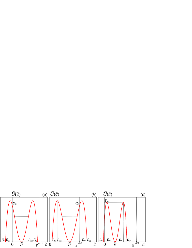
Figure 1: The form of the field $\tilde{U}(\tilde{c})$ at different values of average concentration and temperature. (​a) $0<\overline{c}\leq 1/2$,  $\tau<-\,\overline{c}^{\,2}\!\big{/}g$,  (​b) $1/2\leq\overline{c}<1$,  $\tau<-(1-\overline{c})^{2}\!\big{/}g$   (​W -phase),  (​c) $0<\overline{c}\leq 1/2$,  $\tau\geq-\,\overline{c}^{\,2}\!\big{/}g$; $1/2\leq\overline{c}<1$,  $\tau\geq-(1-\overline{c})^{2}\!\big{/}g$   (K -phase).

Thus, along with the homogeneous H -phase, the stable inhomogeneous K -  and W - phases can exist in binary solutions.

IV Free energy parameters

Further consideration will be based on the expansion of the free energy in powers of the concentration fluctuations (8). To estimate the phenomenological parameters entering in (5), (6) and find their dependence on the average concentration, temperature and density, we use the well-known representation of the free energy AGK ; MT , which in the considered case of an isotropic medium can be represented as

$$\begin{array}[]{l}\displaystyle{\overline{F}=\frac{n^{2}}{2}\!\int\!d{\bf r}d{\bf r}^{\prime}V\big{(}|{\bf r}-{\bf r}^{\prime}|\big{)}c({\bf r})c({\bf r}^{\prime})+nT\!\int\!d{\bf r}\Big{[}c({\bf r})\ln c({\bf r})+\big{(}1-c({\bf r})\big{)}\ln\big{(}1-c({\bf r})\big{)}\Big{]},}\end{array}$$ (22)

where $V\big{(}|{\bf r}-{\bf r}^{\prime}|\big{)}$ is the interaction potential between particles. Expanding (22) in small fluctuations $\delta c({\bf r})=c({\bf r})-\overline{c}$ and comparing with (4) – (6), we obtain the following expressions for the expansion coefficients:

$$\begin{array}[]{ccc}\displaystyle{a_{2}=nV_{0}+\frac{T}{\overline{c}\,(1-\overline{c})},\qquad a_{3}=-\frac{(1-2\overline{c})}{2\,\overline{c}^{\,2}(1-\overline{c})^{2}}\,T,\qquad a_{4}=\frac{(1-3\overline{c}+3\overline{c}^{\,2})}{3\,\overline{c}^{\,3}(1-\overline{c})^{3}}\,T,\vspace{2mm}}\\ \displaystyle{K=-\frac{2\pi}{3}\,n\!\int\!dr\,r^{4}V(r),\qquad\varphi_{0}(T,\overline{c})=\frac{\overline{c}^{\,2}n}{2}\,V_{0}+T\big{[}\,\overline{c}\ln\overline{c}+(1-\overline{c})\ln(1-\overline{c})\big{]},}\end{array}$$ (23)

where $V_{0}=\!\int d{\bf r}V(r)$. When calculating the gradient contribution, we used the expansion $\delta c({\bf r}+{\boldsymbol{\uprho}})\approx\delta c({\bf r})+\rho_{i}\nabla_{i}\,\delta c({\bf r})+\frac{1}{2}\rho_{i}\rho_{k}\nabla_{i}\nabla_{k}\,\delta c({\bf r})$ in the first term in (22), and also took into account that in an isotropic medium

$$\begin{array}[]{ccc}\displaystyle{\int\!d{\boldsymbol{\uprho}}\,\rho_{i}V(\rho)=0,\qquad\int\!d{\boldsymbol{\uprho}}\,\rho_{i}\rho_{k}V(\rho)=\delta_{ik}\,\frac{1}{3}\int\!d\rho\,\rho^{2}V(\rho).}\end{array}$$ (24)

As is seen, the coefficient $a_{2}$ can change sign at a certain temperature, becoming negative if only $V_{0}<0$, so that the possibility of a loss of stability is determined by the character of the interaction between atoms. In the potential of interparticle interaction, as a rule, it is possible to distinguish the region of repulsion at small distances and the region of attraction at large distances. For many model potentials it is assumed that the repulsion at small distances becomes infinitely large, which turns out to be inconvenient in theoretical studies. However, it is quite admissible and natural to consider effective potentials that remain finite at small distances YP1 ; PS . For further estimates we will use the modified Sutherland potential

$$\begin{array}[]{ll}\displaystyle{V(r)=\left\{\begin{array}[]{l}\,\,\,\,v_{0},\qquad\qquad\quad r<r_{0},\vspace{3mm}\\ \displaystyle{-\,v_{m}\!\left(\frac{r_{0}}{r}\right)^{\!6},\quad\,\,\,\,r>r_{0},}\end{array}\right.}\end{array}$$ (25)

where $v_{0}>0$ and $v_{m}>0$. For this potential we obtain

$$\begin{array}[]{l}\displaystyle{V_{0}=\frac{4\pi}{3}r_{0}^{3}(v_{0}-v_{m}),\qquad K=-\frac{2\pi}{15}\,nr_{0}^{5}(v_{0}-5v_{m}).}\end{array}$$ (26)

For a sufficiently deep well in the potential (25) $v_{m}>v_{0}$, there holds the condition $V_{0}<0$. In this case it is also ensured the condition of stability of the homogeneous state $K>0$. The spinodal decomposition temperature is then determined by the formula

$$\begin{array}[]{l}\displaystyle{T_{p}=n|V_{0}|\,\overline{c}\,(1-\overline{c}).}\end{array}$$ (27)

In the coefficient $a_{2}=a_{0}\tau$ the proportionality parameter is

$$\begin{array}[]{l}\displaystyle{a_{0}\equiv\frac{T_{p}}{\overline{c}\,(1-\overline{c})}=n|V_{0}|.}\end{array}$$ (28)

Let us also present expressions for the dimensionless parameters (12):

$$\begin{array}[]{ccc}\displaystyle{g\equiv g(\tau,\overline{c})=\frac{g_{0}(\overline{c})}{(1+\tau)},\qquad g_{0}(\overline{c})\equiv\frac{3\overline{c}^{\,2}(1-\overline{c})^{2}}{(1-3\overline{c}+3\overline{c}^{\,2})},\vspace{2mm}}\\ \displaystyle{b\equiv-(1+\tau)^{1\!/2}b_{0}(\overline{c}),\qquad b_{0}(\overline{c})\equiv\frac{\sqrt{3}}{2}\frac{(1-2\overline{c})}{(1-3\overline{c}+3\overline{c}^{\,2})^{1\!/2}}.}\end{array}$$ (29)

For completeness we gave a formula for the coefficient $b$, although, as was said, it is omitted in this work. The correlation length for potential (25) is given by the formula

$$\begin{array}[]{ccc}\displaystyle{\xi_{0}^{2}=\frac{2\pi}{3V_{0}}\!\int\!d\rho\,\rho^{4}V(\rho)=r_{0}^{2}\frac{(v_{m}-v_{0}/5)}{2(v_{m}-v_{0})},}\end{array}$$ (30)

and is of the order of magnitude of the radius of action of the interparticle potential $\xi_{0}\sim r_{0}$. The macroscopic description and expansion in terms of small concentration gradients is valid if the characteristic distance at which the concentration changes $L_{c}$ is much larger than the correlation length $L_{c}\gg\xi_{0}$. We also note that to analyze nonlinear effects we use the expansion in powers of concentration (8), without imposing restrictions on the magnitude of the concentration fluctuations.

V Phase diagram

Bounded solutions of Eq. (17) exist in the range of variation of the parameter $0\leq\varepsilon\leq\varepsilon_{m}$. As noted above, depending on the values of $\tau$ and $\overline{c}$ there are two possibilities. First, at permissible concentration values the parameter $\varepsilon$ can take its maximum value equal to the field maximum $\varepsilon_{m}=\tilde{U}(\tilde{c}_{m1})=\tilde{U}(\tilde{c}_{m2})=|\tau|^{2}\!\big{/}4$ (Fig. 1c). In this case, at $\varepsilon=\varepsilon_{m}$ the solution of Eq. (17) has the form of a kink

$$\begin{array}[]{ccc}\displaystyle{\delta\tilde{c}(\tilde{x})=\tilde{c}(\tilde{x})-\tilde{\overline{c}}=\pm\sqrt{|\tau|}\,\,{\rm th}\!\!\left(\!\frac{\sqrt{|\tau|}\,\tilde{x}}{\sqrt{2}}\right).}\end{array}$$ (31)

This formula describes a solution, in which with a change of the coordinate a transition occurs from the homogeneous state with an increased concentration to the homogeneous state where the concentration is less than the average one, so that $c(+\infty)-c(-\infty)=2\sqrt{g|\tau|}$. The solution stratifies into two areas, in which the concentration is above and below the average one. The width of the transition region, where the concentration changes significantly, is given by the formula $L_{K}=\sqrt{\frac{2}{|\tau|}}\,\xi_{0}$. At $\tau\rightarrow 0$ the concentration difference tends to zero and the width of the transition region tends to infinity, so that in the result the system goes over to the spatially homogeneous state.

In the range of variation of the parameter $0<\varepsilon<\varepsilon_{m}$, the solution has the form of a concentration wave

$$\begin{array}[]{ccc}\displaystyle{\delta\tilde{c}(\tilde{x})=\tilde{c}(\tilde{x})-\tilde{\overline{c}}=\pm\,D_{-}\,{\rm sn}\!\left(\!\frac{\tilde{x}}{\sqrt{2}}\,D_{+},m\right),}\end{array}$$ (32)

where $\displaystyle{D_{\pm}\equiv D_{\pm}(\tau,\varepsilon)\equiv\sqrt{|\tau|\pm\sqrt{\tau^{2}-4\varepsilon}}}$, $m\equiv m(\tau,\varepsilon)=D_{-}^{2}\big{/}D_{+}^{2}$, ${\rm sn}\!\left(\!\frac{\tilde{x}D_{+}}{\sqrt{2}},m\right)$ is the elliptic sine function AS . The description of the distribution of atoms of a solid solution by means of concentration waves was proposed by Krivoglaz MK and developed in relation to the description of ordered solutions in AGK . In the limit $\varepsilon\rightarrow|\tau|^{2}\!\big{/}4$ or $m\rightarrow 1$, this solution goes over to the kink solution (31). The case $\varepsilon=0$ corresponds to the spatially homogeneous state. The solution with the maximum possible value $\varepsilon=\varepsilon_{m}$ in the form of a kink (31) corresponds to the minimum value of the free energy.

In another possible case, the maximum value of the parameter $\varepsilon=\varepsilon_{m}$ at all permissible concentrations is less than the maximum value of the field $\varepsilon_{m}<|\tau|^{2}\!\big{/}4$ (Fig. 1a,b). At $\overline{c}\leq 1/2$   $\displaystyle{\varepsilon_{m}=\tilde{U}(0,\tau)=-\frac{\overline{c}^{\,2}}{4g}\left(\frac{\overline{c}^{\,2}}{g}+2\tau\right)}$, and at $\overline{c}\geq 1/2$   $\displaystyle{\varepsilon_{m}=\tilde{U}\left(\frac{1}{\sqrt{g}},\tau\right)=-\frac{(1-\overline{c})^{2}}{4g}\left(\frac{(1-\overline{c})^{2}}{g}+2\tau\right)}$. In this case, there is no solution in the form of a kink and all bounded solutions at $0<\varepsilon\leq\varepsilon_{m}$ have the form of concentration waves (32).

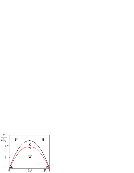
Figure 2: Phase diagram in the coordinates $\big{(}\overline{c},T\!\big{/}n|V_{0}|\big{)}$. The lines $a_{1}ca_{2}$, $a_{1}b$, $ba_{2}$ respectively correspond to the dependencies: $T_{p}\big{/}n|V_{0}|=\overline{c}\,(1-\overline{c})$, $T_{1}\!\big{/}n|V_{0}|=3\overline{c}\,(1-\overline{c})^{3}\!\big{/}(4-9\overline{c}+6\overline{c}^{\,2})$, $T_{2}\big{/}n|V_{0}|=3\overline{c}^{\,3}(1-\overline{c})\!\big{/}(1-3\overline{c}+6\overline{c}^{\,2})$. Above the curve $a_{1}ca_{2}$ there is the homogeneous H -phase. Inside the area $a_{1}ca_{2}b$ is the K -phase. Inside the area $a_{1}ba_{2}$ is the W -phase.

As we can see, while at $\tau\geq 0$ there is only the spatially homogeneous H -phase, at $\tau<0$ there are two qualitatively different states. In one of them, in addition to the solutions in the form of concentration waves, there exists the solution in the form of a kink (31), which actually corresponds to the smallest value of the free energy. We called this state the K -phase. In this phase the solution is stratified into two spatial regions with increased and depleted concentrations. In the other phase all solutions have the form of concentration waves (32), and there is no solution in the form of a kink. We called this state the W -phase. The phase diagram in the coordinates temperature – average concentration is shown in Fig. 2. Note that at $\overline{c}\rightarrow 0$ we have $T_{p}\sim\overline{c}$, and at $\overline{c}\rightarrow 1$ we have $T_{p}\sim(1-\overline{c})$, so that the transition temperature tends to zero in both limiting cases. Here, generally speaking, due to the proximity of $T_{p}$ to absolute zero the applicability of the model and the used classical description may be violated.

The concentration distributions in the inhomogeneous phases during stratification (a) and in the concentration wave (b) are shown in Fig. 3. As is seen, transitions between the phases are accompanied by the transfer of a significant amount of matter. In this work, however, we do not consider the kinetics of transitions between the phases and do not estimate the characteristic times during which such transitions occur, but we study only thermodynamically equilibrium states.

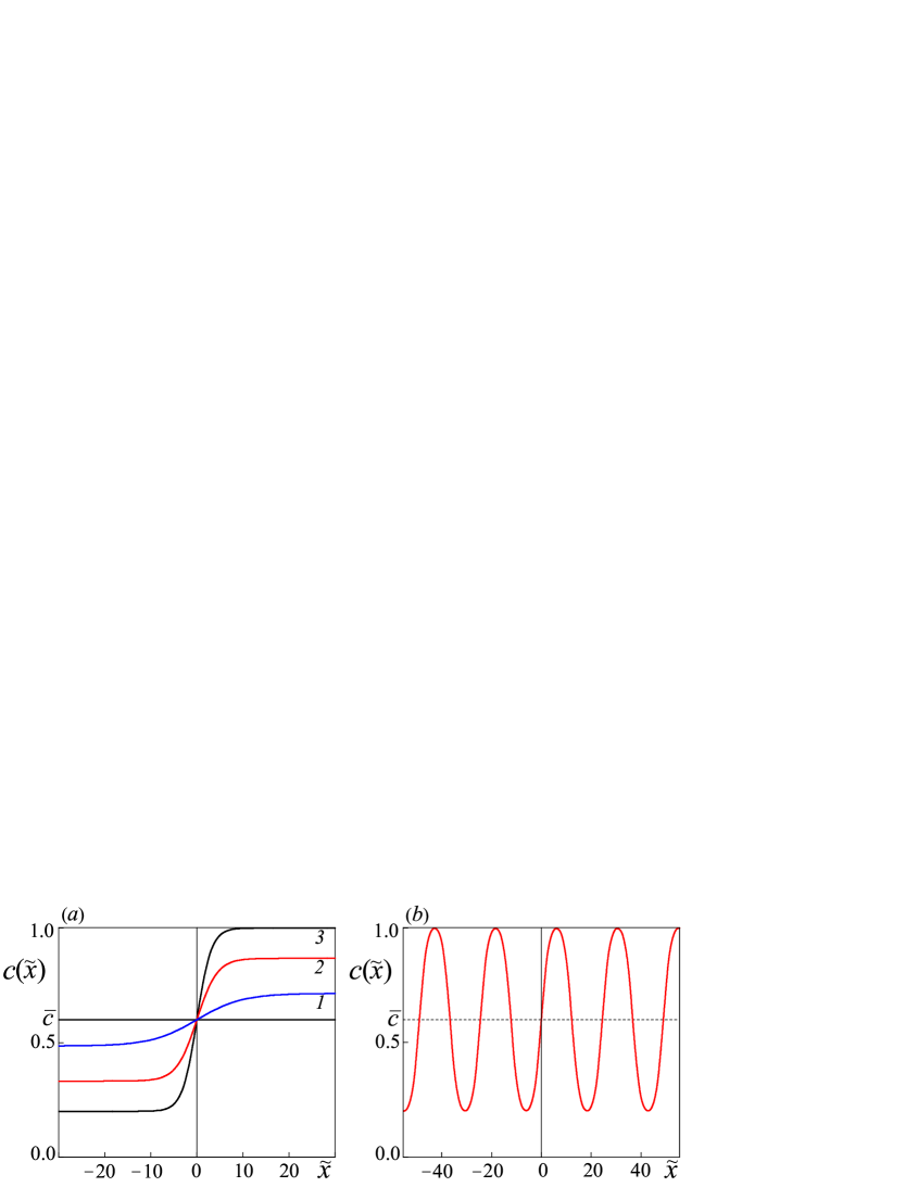
Figure 3: (​a) The concentration distributions $c(\tilde{x})_{K}$ in the K -phase ($\tilde{T}_{2}\leq\tilde{T}<\tilde{T}_{p}=0.24$) at temperatures $\tilde{T}=T\!\big{/}n|V_{0}|$ : 1 –  $\tilde{T}=0.235$, 2 –  $\tilde{T}=0.215$, 3 –  $\tilde{T}_{2}=0.191$. The line $c=\overline{c}=0.6$ corresponds to the H -phase at $\tilde{T}\geq\tilde{T}_{p}$. (​b) The concentration distribution $c(\tilde{x})_{W}$ in the W -phase $(\tilde{T}<\tilde{T}_{2})$ at $\tilde{T}=0.185$.

VI Thermodynamics of inhomogeneous states

Let us calculate the contribution of inhomogeneity to the thermodynamic functions of the phases and analyze the character of transitions between the phases. Substituting the solution at a certain value of $\varepsilon$ into (8), we find the contribution of this state to the equilibrium free energy. For the kink in the limit $L\rightarrow\infty$, we obtain

$$\begin{array}[]{ccc}\displaystyle{\frac{F}{a_{4}g^{2}N}=-\varepsilon=-\frac{\tau^{2}}{4}.}\end{array}$$ (33)

For the concentration wave at a certain value of $\varepsilon$, we have

$$\begin{array}[]{ccc}\displaystyle{\frac{F(\tau,\varepsilon)}{a_{4}g^{2}N}=\frac{1}{3}\!\left[\varepsilon+\tau D_{+}^{2}(\tau,\varepsilon)\left(1-\frac{E(m)}{K(m)}\right)\right],}\end{array}$$ (34)

where $K(m),E(m)$ are the complete elliptic integrals of the first and second kind AS . In the following, in (34) it is more convenient to express the parameter $\varepsilon$ in terms of the parameter

$$\begin{array}[]{ccc}\displaystyle{m=\frac{|\tau|-\sqrt{\tau^{2}-4\varepsilon}}{|\tau|+\sqrt{\tau^{2}-4\varepsilon}},}\end{array}$$ (35)

which varies from $m=0$ at $\varepsilon=0$ to $m=m_{*}(\tau)\equiv\displaystyle{\Big{(}|\tau|-\sqrt{\tau^{2}-4\varepsilon_{m}}\Big{)}\!\Big{/}\!\Big{(}|\tau|+\sqrt{\tau^{2}-4\varepsilon_{m}}}\Big{)}$ at $\varepsilon=\varepsilon_{m}$. So we find the energy of the inhomogeneous state per one particle

$$\begin{array}[]{ccc}\displaystyle{\frac{F(\tau,m)}{N}=-G\tau^{2}f(m),}\end{array}$$ (36)

where the function

$$\begin{array}[]{ccc}\displaystyle{f(m)\equiv\frac{(2+m)}{(1+m)^{2}}-\frac{2}{(1+m)}\frac{E(m)}{K(m)}}\end{array}$$ (37)

is defined, and $G\equiv\frac{1}{3}a_{4}g^{2}$ is a constant which with taking into account the formulas (23), (27), (29) can be presented in the form

$$\begin{array}[]{ccc}\displaystyle{G=T_{p}\frac{\eta(\overline{c})}{(1+\tau)},\qquad\eta(\overline{c})\equiv\frac{\overline{c}(1-\overline{c})}{(1-3\overline{c}+3\overline{c}^{\,2})}.}\end{array}$$ (38)

The form of the function (37) is shown in Fig. 4. It is positive and increases from $f(0)=0$ to $f(1)=3/4$, and a very rapid growth occurs at $m\approx 1$, so that here the derivative goes to infinity.

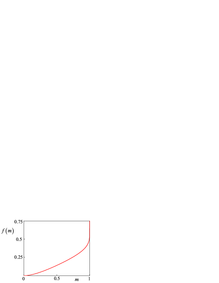
Figure 4: Form of the function $f(m)$ (37).

The function $F(\tau,m)$ (36) determines the contribution of solution with index $m$ to the energy. If excitations with different energies are possible in a physical system, then all of them contribute to the total equilibrium free energy. According to the general principles of statistical physics, the probability of finding the system in the state with the parameter $m$ in the interval $m\div m+dm$

$$\begin{array}[]{ccc}\displaystyle{dw=\phi(T,m)\,dm}\end{array}$$ (39)

is determined by means of the “one-particle” distribution function over states $m$

$$\begin{array}[]{ccc}\displaystyle{\phi(T,m)\equiv\frac{e^{-\frac{F(\tau,m)}{NT}}}{Z}=\frac{e^{B(\tau)f(m)}}{Z},}\end{array}$$ (40)

where we use the notation

$$\begin{array}[]{ccc}\displaystyle{B(\tau)\equiv\frac{\tau^{2}}{(1+\tau)^{2}}\,\eta(\overline{c}).}\end{array}$$ (41)

The statistical integral is determined by the normalization condition $\int_{0}^{m_{*}(\tau)}\!\!\phi(T,m)\,dm=1$:

$$\begin{array}[]{ccc}\displaystyle{Z=\int\limits_{0}^{m_{*}(\tau)}e^{B(\tau)f(m)}dm.}\end{array}$$ (42)

The average of an arbitrary function $A=A(m)$ is given by the formula

$$\begin{array}[]{ccc}\displaystyle{\big{\langle}A\big{\rangle}=\int\limits_{0}^{m_{*}(\tau)}A(m)\phi(\tau,m)dm.}\end{array}$$ (43)

As follows from the form of the function (37) (Fig. 4), the largest contribution is made by the state with the maximum value $m=m_{*}$, while the contribution of the states with smaller values of $m$ rapidly decreases.

The average value of the function (36) determines the contribution of inhomogeneous states to the average energy

$$\begin{array}[]{ccc}\displaystyle{E=\int\limits_{0}^{m_{*}}F(\tau,m)\phi(\tau,m)dm=-NG\,\tau^{2}\big{\langle}f\big{\rangle}.}\end{array}$$ (44)

The contribution to the total entropy due to inhomogeneity of states is determined through the average of the logarithm of the distribution function LL , so that the entropy per one particle is given by the formula

$$\begin{array}[]{ccc}\displaystyle{\frac{S}{N}\equiv-\big{\langle}\ln\phi\,\big{\rangle}=\ln Z-B\big{\langle}f\big{\rangle}.}\end{array}$$ (45)

The contribution of inhomogeneity to the total heat capacity can be determined through the derivative of the entropy

$$\begin{array}[]{ccc}\displaystyle{\frac{C}{N}=\frac{T}{N}\frac{dS}{dT}=\frac{2\,\tau^{3}}{(1+\tau)^{4}}\,\eta^{2}(\overline{c})\Big{(}\!\big{\langle}f\big{\rangle}^{2}-\big{\langle}f^{\,2}\big{\rangle}\!\Big{)}+(1+\tau)\frac{e^{Bf(m_{*})}}{Z}\!\left[1+\frac{\tau^{2}}{(1+\tau)^{2}}\,\eta(\overline{c})\Big{(}\!\big{\langle}f\big{\rangle}-f(m_{*})\Big{)}\right]\!\frac{dm_{*}}{d\tau}\,,}\end{array}$$ (46)

where

$$\begin{array}[]{ccc}\displaystyle{\big{\langle}f^{\,n}\big{\rangle}=\int\limits_{0}^{m_{*}}\,\big{[}f(m)\big{]}^{n}\phi(\tau,m)\,dm.}\end{array}$$ (47)

In particular, in the K -phase  $m_{*}=1$, and in the W -phase

$$\begin{array}[]{ccc}\displaystyle{m_{*}(\tau)=\frac{(\tau+1)}{\tau\!\left(\!\displaystyle{\frac{2}{\tau_{i}}}+1\!\right)\!-1},\qquad\frac{dm_{*}}{d\tau}=-\frac{2\,(\tau_{i}+1)}{\tau_{i}\!\left[\tau\!\left(\!\displaystyle{\frac{2}{\tau_{i}}}+1\!\right)\!-1\right]^{\!2}}.}\end{array}$$ (48)

Here at $0<\overline{c}\leq 1/2$   $i=1$, and at $1/2\leq\overline{c}<1$   $i=2$, and at that

$$\begin{array}[]{ccc}\displaystyle{\tau_{1}=\frac{T_{1}-T_{p}}{T_{p}}=-\frac{\overline{c}^{\,2}}{\left[\overline{c}^{\,2}+g_{0}(\overline{c})\right]},\qquad\tau_{2}=\frac{T_{2}-T_{p}}{T_{p}}=-\frac{(1-\overline{c})^{2}}{\left[(1-\overline{c})^{2}+g_{0}(\overline{c})\right]}.}\end{array}$$ (49)

The temperature dependences of the contributions of inhomogeneous states to the entropy and heat capacity are shown in Fig. 5.

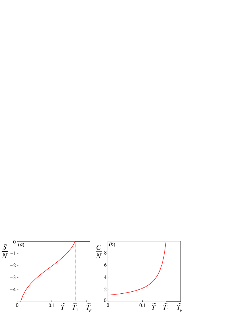
Figure 5: Dependencies of (​a) the entropy and (​b) the heat capacity on the dimensionless temperature $\tilde{T}=T\!\big{/}n|V_{0}|$
($\overline{c}=0.3$, $\tilde{T}_{1}=0.168$, $\tilde{T}_{p}=0.21$).

As we can see, in the K -phase at $\tilde{T}_{1}\leq\tilde{T}<\tilde{T}_{p}$ the entropy and heat capacity associated with inhomogeneity are small, so that on the scale of the figure they are practically close to zero. Upon transition to the W -phase the entropy decreases, and the heat capacity at the transition temperature $\tilde{T}_{1}$ increases by a jump and also decreases monotonically with decreasing temperature. As it was noted, near absolute zero the applicability of the used model and the classical approach may be violated.

The existence, along with the main solutions determining the structure of the phases, also of other solutions in the form of concentration waves with energies greater than the energy of the main solution, will somewhat affect the concentration distribution in the phases, but due to the randomness of phases this will not lead to a qualitative change in the form of the concentration distributions in the K -  and W -phases shown in Fig. 3.

It is important to note that a loss of stability of the homogeneous state is described by the solution of the nonlinear equation in the form of a kink (31) even near $T_{p}$. Thus, to analyze a loss of stability it is not enough applying a linear approximation, and taking into account nonlinear effects proves to be important even for small $\tau$.

VII Phase transition from the H -phase to the K -phase

As can be seen from the phase diagram in Fig. 2, with decreasing temperature at $T=T_{p}$ the solution loses its stability and begins to stratify passing to the K -phase. Let us consider in more detail the thermodynamics of this transition. Near the transition from the homogeneous H -phase to the K -phase, where $|\tau|\ll 1$ and $B\approx\eta(\overline{c})\tau^{2}<1$, from (45) and (46) there follow formulas for the entropy and heat capacity:

$$\begin{array}[]{ccc}\displaystyle{\frac{S}{N}=\frac{\big{[}\eta(\overline{c})\big{]}^{2}}{2}\big{(}f_{1}^{\,2}-f_{2}\big{)}\hskip 0.85358pt\tau^{4},}\end{array}$$ (50)

$$\begin{array}[]{ccc}\displaystyle{\frac{C}{N}=2\big{[}\eta(\overline{c})\big{]}^{2}\big{(}f_{1}^{\,2}-f_{2}\big{)}\hskip 0.85358pt\tau^{3}.}\end{array}$$ (51)

Here $f_{n}=\int_{0}^{1}\!\big{[}f(m)\big{]}^{n}dm$ and $f_{1}\approx 0.162$, $f_{2}\approx 0.043$, $f_{1}^{\,2}-f_{2}=-0.017$. Thus, there occurs a smooth phase transition from the homogeneous state to the phase where the solution is stratified. In this case in the inhomogeneous state the entropy slightly decreases and the heat capacity increases (Fig. 5). Only the fourth derivative of the entropy with respect to temperature experiences a jump. The form of the temperature dependences (50) and (51) is mainly determined by the fact that the linear approximation of the dependence of the coefficient $a_{2}=a_{0}(T-T_{p})/T_{p}$ in (6) on temperature was used. As is known LL ; HS ; PP , near the phase transition temperature, fluctuations begin to play an important role, which are not taken into account in this approach based on the mean field theory. An effective account for fluctuations should lead to a modification of the critical exponents and temperature dependences of quantities near the phase transition GS ; YP2 .

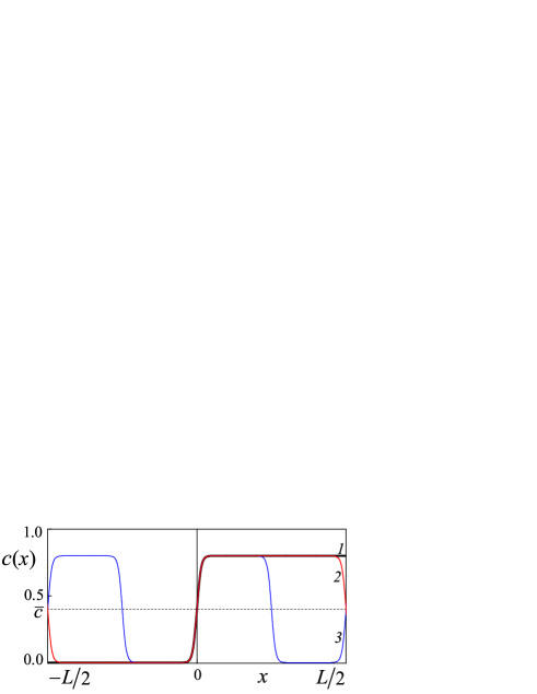
Figure 6: Evolution of the concentration distribution during the transition of the stratified solution into the phase with concentration waves. Curve 1 is the distribution at the transition boundary at $\tilde{T}=\tilde{T}_{1}$. Curves 2 and 3 are the distributions in the W -phase at $\tilde{T}<\tilde{T}_{1}$, with respectively one and two wave periods at the sample length $L$. Parameters: $\overline{c}=0.4,\,\tilde{T}_{1}=0.191$.

VIII Phase transition between inhomogeneous phases

As it was noted earlier (Fig. 2), below the temperature $T_{p}$ after a loss of stability of the homogeneous phase there first appears the K -phase and the stratification of the solution occurs. The phase with stratification exists in the temperature range $T_{1}\leq T<T_{p}$ if $\overline{c}\leq 1/2$, and $T_{2}\leq T<T_{p}$ if $\overline{c}\geq 1/2$, where

$$\begin{array}[]{ccc}\displaystyle{T_{1}=T_{p}\frac{3(1-\overline{c})^{2}}{(4-9\overline{c}+6\overline{c}^{\,2})},\qquad T_{2}=T_{p}\frac{3\overline{c}^{\,2}}{(1-3\overline{c}+6\overline{c}^{\,2})}.}\end{array}$$ (52)

At lower temperatures $0<T<T_{1}$ if  $\overline{c}\leq 1/2$, and $0<T<T_{2}$ if  $\overline{c}\geq 1/2$, the W -phase appears (Fig. 2). Figure 6 shows the evolution of the concentration distribution near the transition from the stratified state to the state with a concentration wave. With a further decrease in temperature the concentration wave takes a shape close to sinusoidal (Fig. 3b).

Let us consider in more detail the character of the transition from the K -phase to the W -phase. In the region of existence of the K -phase the entropy and heat capacity can be represented in the form

$$\begin{array}[]{ccc}\displaystyle{\frac{S_{K}(\tau)}{N}=\ln Z_{K}-\frac{\tau^{2}}{(1+\tau)^{2}}\,\eta(\overline{c})\big{\langle}f\big{\rangle}_{\!K},}\end{array}$$ (53)

$$\begin{array}[]{ccc}\displaystyle{\frac{C_{K}(\tau)}{N}=\frac{2\,\tau^{3}}{(1+\tau)^{4}}\,\eta^{2}(\overline{c})\Big{(}\!\big{\langle}f\big{\rangle}_{\!K}^{2}-\big{\langle}f^{\,2}\big{\rangle}_{\!K}\!\Big{)},}\end{array}$$ (54)

where

$$\begin{array}[]{ccc}\displaystyle{Z_{K}=\int\limits_{0}^{1}\!e^{Bf(m)}dm,\qquad\big{\langle}f\big{\rangle}_{\!K}=\frac{1}{Z_{K}}\int\limits_{0}^{1}\!f(m)\hskip 1.42262pte^{Bf(m)}dm,\qquad\big{\langle}f^{\,2}\big{\rangle}_{\!K}=\frac{1}{Z_{K}}\int\limits_{0}^{1}\!f^{\,2}(m)\hskip 1.42262pte^{Bf(m)}dm.}\end{array}$$ (55)

In the W -phase with concentration waves the same quantities have the form

$$\begin{array}[]{ccc}\displaystyle{\frac{S_{W}(\tau)}{N}=\ln Z_{W}-\frac{\tau^{2}}{(1+\tau)^{2}}\,\eta(\overline{c})\big{\langle}f\big{\rangle}_{\!W},}\end{array}$$ (56)

$$\begin{array}[]{ccc}\displaystyle{\frac{C_{W}(\tau)}{N}=\frac{2\,\tau^{3}}{(1+\tau)^{4}}\,\eta^{2}(\overline{c})\Big{(}\!\big{\langle}f\big{\rangle}_{\!W}^{2}-\big{\langle}f^{\,2}\big{\rangle}_{\!W}\!\Big{)}+(1+\tau)\frac{e^{Bf(m_{*})}}{Z_{W}}\!\left[1+\frac{\tau^{2}}{(1+\tau)^{2}}\,\eta(\overline{c})\Big{(}\!\big{\langle}f\big{\rangle}_{\!W}-f(m_{*})\Big{)}\right]\!\frac{dm_{*}}{d\tau}\,,}\end{array}$$ (57)

where

$$\begin{array}[]{ccc}\displaystyle{Z_{W}=\int\limits_{0}^{m_{*}}\!e^{Bf(m)}dm,\qquad\big{\langle}f\big{\rangle}_{\!W}=\frac{1}{Z_{W}}\int\limits_{0}^{m_{*}}\!f(m)\hskip 1.42262pte^{Bf(m)}dm,\qquad\big{\langle}f^{\,2}\big{\rangle}_{\!W}=\frac{1}{Z_{W}}\int\limits_{0}^{m_{*}}\!f^{\,2}(m)\hskip 1.42262pte^{Bf(m)}dm.}\end{array}$$ (58)

The parameter $m_{*}$ is defined by the formula (48). The calculation shows that the entropy and heat capacity in the W -phase are much higher than the values of the same quantities in the K -phase, so that in Fig. 5 where the temperature dependences of these quantities are presented, as it was noted, on the used scale they are close to zero. Attention is drawn to the curious fact that when approaching zero temperature, the contribution of the concentration wave to the heat capacity per one particle proves to be close to unity at various average concentrations.

At the K  -W transition, the entropy turns out to be continuous and the heat capacity undergoes a jump

$$\begin{array}[]{ccc}\displaystyle{\frac{\Delta C}{N}\equiv\frac{C_{W}-C_{K}}{N}=\frac{2}{|\tau_{i}|}\frac{e^{B(\tau_{i})f(1)}}{Z_{K}(\tau_{i})}\!\left[1+B(\tau_{i})\Big{(}\!\big{\langle}f\big{\rangle}_{\!K}-f(1)\Big{)}\right],\quad\,\,(i=1,2).}\end{array}$$ (59)

Thus, the transition between the K -  and W - phases is a second-order transition. Figure 7 shows the dependence of the magnitude of the jump in the heat capacity on the average concentration.

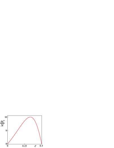
Figure 7: Dependence of the jump in the heat capacity $\Delta C=C_{W}(T_{1})-C_{K}(T_{1})$ at the transition between the K -  and W - phases on the average concentration.

Note that the jump in the heat capacity remains finite even in the limit of low concentrations, although, as mentioned above, the condition of applicability of the model and the classical description of the solution may be violated here.

IX Conclusion

The thermodynamics of equilibrium phase transitions of the binary solution into spatially inhomogeneous states is investigated theoretically taking into account nonlinear effects. It is shown that as a result of a loss of stability of the homogeneous H -phase with decreasing temperature, at first there occurs the stratification of the solution for which the concentration distribution is described by the dependence in the form of a kink (31) (the K -phase). After reaching the maximum possible stratification at a lower temperature there occurs a second-order phase transition into the state with a concentration wave which is described by the periodic solution (32) (the W -phase). The function of distribution of states in the inhomogeneous solution is introduced and with its help the contribution of inhomogeneity to the entropy and heat capacity is calculated. The phase diagram in the coordinates temperature – average concentration is constructed. The proposed approach can be used to describe transitions into spatially inhomogeneous phases in other many-particle systems.

List of Notations

$N$	total number of particles
$N_{1},N_{2}$	numbers of particles of two types
$n$	total density of number of particles
$V$	volume of a solution
$T$	temperature
$\overline{c}=c_{1}$	average concentration of the first component
$c=c({\bf r})$	local concentration of the first component
$\delta c({\bf r})$	deviation of the concentration from the average value
$\varphi$	free energy per one particle
$\varphi_{0}$	contribution of the homogeneous state to $\varphi$
$\overline{F}$	total free energy in the state of incomplete thermodynamic equilibrium
$F$	total free energy in the equilibrium state
$K,a_{2},a_{3},a_{4}$	coefficients in the expansion of $\varphi$ in $\big{(}\nabla\delta c\big{)}^{2}$ and powers of $\delta c$
$T_{p}$	temperature at which the coefficient $a_{2}$ changes sign
$\tau=(T-T_{p})\big{/}T_{p}$	parameter of dimensionless temperature, such that $a_{2}=a_{0}\tau$
$L,A$	length and area of a sample
$x$	one spatial coordinate on which the concentration depends
$U(\delta c),C$	effective field and constant of integration in the equation for $\delta c$
$\tilde{c}=g^{-1/2}c$	reduced concentration
$\tilde{\overline{c}}=g^{-1/2}\overline{c}$	reduced average concentration
$\delta\tilde{c}=\tilde{c}-\tilde{\overline{c}}$	reduced deviation of the concentration from the average value
$\tilde{x}=x/\xi_{0}$	dimensionless coordinate, where $\xi_{0}$ is the correlation length
$g,b,\varepsilon$	dimensionless parameters, defined by the formula (12)
$\tilde{U}(\delta\tilde{c};b,\tau)$	reduced effective field, given by the formula (15)
$\tilde{U}(\tilde{c};\tilde{\overline{c}},b,\tau)$	reduced effective field as a function of $\tilde{c}$, given by (18) in general case
	and by (19) in the case $b=0$
$\tilde{c}_{m1},\tilde{c}_{m2}$	maximums of $\tilde{U}(\tilde{c})$ for the case $b=0$
$\tilde{c}_{01},\tilde{c}_{02}$	zeros of $\tilde{U}(\tilde{c})$ for the case $b=0$
$V\big{(}|{\bf r}-{\bf r}^{\prime}|\big{)}$	interaction potential between particles
$V_{0}=\!\int d{\bf r}V(r)$	constant relating to the interaction potential
$v_{0},v_{m},r_{0}$	constants of the potential $V(r)$, defined by the formula (25)
$\varepsilon_{m}$	maximum possible value of the parameter $\varepsilon$
$L_{K}$	width of the transition region in the kink (31)
$m(\tau,\varepsilon)$	parameter (35) entering into the elliptic functions and integrals
$m_{*}(\tau)$	$m(\tau,\varepsilon_{m})$, i.e. maximum value of $m$ at given $\tau$
$\phi(T,m)$	“one-particle” distribution function over states $m$
$f(m)$	characteristic function (37)
$E$	average energy contribution due to inhomogeneous states
$S$	entropy contribution due to inhomogeneous states
$C$	heat capacity contribution due to inhomogeneous states
$T_{1},T_{2}$	temperatures of the phase transition between the inhomogeneous
	K -  and W -phases, given by the formula (52)
$\Delta C$	jump of the heat capacity at the K  -W transition, given by (59)

References

• (1) A.G. Khachaturian, Theory of phase transformations and structure of solid solutions, Nauka, Moscow, 384 p. (1974).
• (2) B.N. Eselson, V.N. Grigor’ev, V.G. Ivantsov, E.Ya. Rudavskii, D.G. Sanikidze, I.A. Serbin, Solutions of 3He – 4He quantum liquids, Nauka, Moscow, 424 p. (1973).
• (3) V.P. Skripov, A.V. Skripov, Spinodal decomposition (phase transitions via unstable states), Sov. Phys. Usp. 22, 389 (1979). doi:10.1070/PU1979v022n06ABEH005571
• (4) J.W. Cahn, J.E. Hilliard, Free energy of a nonuniform system. I. Interfacial free energy, J. Chem. Phys. 28, 258 (1958). doi:10.1063/1.1744102
• (5) J.W. Cahn, J.E. Hilliard, Free energy of a nonuniform system. II. Thermodynamic basis, J. Chem. Phys. 30, 1121 (1959). doi:10.1063/1.1730145
• (6) J.W. Cahn, J.E. Hilliard, Free energy of a nonuniform system. III. Nucleation in a two-component incompressible fluid, J. Chem. Phys. 31, 688 (1959). doi:10.1063/1.1730447
• (7) M. Hillert, A solid-solution model for inhomogeneous systems, Acta Metallurgica 9, 525 (1961). doi:10.1016/0001-6160(61)90155-9
• (8) L.D. Landau, E.M. Lifshitz, Statistical physics: Vol. 5 (Part 1), Butterworth-Heinemann, 544 p. (1980).
• (9) T. Muto, Yu. Takagi, The theory of order-disorder transitions in alloys, Solid State Physics 1, 193 (1955). doi:10.1016/S0081-1947(08)60679-7
• (10) Yu.M. Poluektov, Thermodynamic perturbation theory for classical systems based on self-consistent field model, Ukr. J. Phys. 60, 553 (2015). doi:10.15407/ujpe60.06.0553
• (11) Yu.M. Poluektov, A.A. Soroka, The equation of state and the quasiparticle mass in the degenerate Fermi system with an effective interaction, East Eur. J. Phys. 2, №3, 40 (2015). arXiv:1511.07682v1 [cond-mat.stat-mech]
• (12) M. Abramowitz, I. Stegun (Editors), Handbook of mathematical functions, National Bureau of Standards Applied mathematics Series 55, 1046p. (1964).
• (13) M.A. Krivoglaz, Theory of X-ray and thermal-neutron scattering by real crystals, Plenum Press, New York, 405p. (1969).
• (14) H.E. Stanley, Introduction to phase transitions and critical phenomena, Oxford U.P., New York, 308p. (1971).
• (15) A.Z. Patashinskii, V.L. Pokrovskii, Fluctuation theory of phase transitions, Pergamon Press, New York, 321p. (1979).
• (16) V.L. Ginzburg, A.A. Sobyanin, Superfluidity of helium II near the $\lambda$ point, Sov. Phys. Usp. 31, 289 (1988). doi:10.1070/PU1988v031n04ABEH005746
• (17) Yu.M. Poluektov, The modification of exponents in the Ginzburg-Sobyanin theory of superfluidity, Low Temp. Phys. 45, 1059 (2019). doi:10.1063/1.5125904