On Second-order Optimization Methods for Federated Learning

Abstract

We consider federated learning (FL), where the training data is distributed across a large number of clients. The standard optimization method in this setting is Federated Averaging (FedAvg), which performs multiple local first-order optimization steps between communication rounds. In this work, we evaluate the performance of several second-order distributed methods with local steps in the FL setting which promise to have favorable convergence properties.
We (i) show that FedAvg performs surprisingly well against its second-order competitors when evaluated under fair metrics (equal amount of local computations)—in contrast to the results of previous work. Based on our numerical study, we propose (ii) a novel variant that uses second-order local information for updates and a global line search to counteract the resulting local specificity.

1 Introduction

Federated learning (FL) is a new machine learning paradigm where the used data can not be sent to a central server and the individual clients have to participate in the optimization process (McMahan et al., 2017; Kairouz et al., 2019). These limitations make classical optimization algorithms not directly applicable to FL, which spurred the interest of the optimization community. The high iteration cost—due to the need to communicate for each update—requires algorithms that make as much progress as possible per round of communication. Second-order methods promise to be a class of algorithms which can do this on a suitable class of functions.

The communication cost in the cross-silo federated learning (Kairouz et al., 2019) is between the one of classical distributed optimization and cross-device federated learning. Assuming that clients are reliable and participate in each round, we can formulate a distributed problem of the form:

$$f(\mathbf{w})=\frac{1}{|\mathcal{S}|}\sum_{i\in\mathcal{S}}l_{i}(\mathbf{w})+\frac{\gamma}{2}\lVert\mathbf{w}\rVert_{2}^{2}\,,$$ (1)

with regularization as studied in (Wang et al., 2018) and where all losses $l_{i}(\mathbf{w})$ are convex and $\mathcal{S}$ denoting the set of all clients defining this problem.

The optimization wall-clock time in the cross-device federated learning (Kairouz et al., 2019) setting is dominated by high latency and low bandwidth connections. Often only a fraction of all (stateless) clients participate in each round. This leads to a stochastic approximation of Eq. (1) in the form of

$$f_{t}(\mathbf{w})=\frac{1}{|\mathcal{S}_{t}|}\sum_{i\in\mathcal{S}_{t}}l_{i}(\mathbf{w})+\frac{\gamma}{2}\lVert\mathbf{w}\rVert_{2}^{2}\,,$$ (2)

as the set of participating clients $\mathcal{S}_{t}$ changes at each step $t$. The optimization algorithm nevertheless has to optimize problem (1) to find the global optimum. This setting permits relatively expensive updates as the communication costs usually outweigh the computation costs by far (especially for first-order methods). Such expensive updates can be the ones from second-order methods or even multiple steps of a cheap method. These local steps before synchronizing the updates make classical convergence rates for a non-distributed setting not directly transferable to this setup. The changing nature of Eq. (2) becomes problematic when the optimum on a single client is not the optimum of all clients, e.g. in the realistic case when data is heterogeneous. Here, a better local solution is possibly not helping to solve the global problem. While it is a challenge for distributed algorithms in general, FedAvg facilitates a balance between the quality of the local update and the overall progress by varying the number of local steps, which is more challenging for second order methods which only do few steps to achieve the same progress.

GIANT (Wang et al., 2018) is a proposed distributed second order method to optimize Eq. (1) which has better communication complexity than first-order accelerated gradient descent (Wang et al., 2018, Tab. 1). GIANT calculates an approximation of the Newton update $[\nabla^{2}f(\mathbf{w}^{t})]^{-1}\nabla f(\mathbf{w})$ by using the global gradient and the local Hessians on each client combined with a global backtracking line search over all clients. This involves three rounds of communication which can be considered quite expensive in comparison with for example local SGD (Zinkevich et al., 2010; Stich, 2018) which only needs one communication round and GIANT does not allow local steps. LocalNewton (Gupta et al., 2021) uses only the local gradient and local Hessian for its updates combined with a local backtracking line search. This allows to do multiple local steps before communicating only once for a global update step but with the risk of calculating an update too specific to the client. When we directly apply both methods to the cross-silo federated learning setting defined by Eq. (2), GIANT has a disadvantage compared to other methods by its many communication rounds and LocalNewton can find a solution which is good for the current client but does not decrease the objective function overall.

Contributions. Our contributions can be summarized as:

• We investigate different new variants of distributed second-order optimizers and derive LocalNewton with global line search which is suitable for the federated learning setting, especially with heterogeneous data meaning that each client has a specific data distribution.

• We show empirically that FedAvg with multiple local steps is surprisingly effective in the cross-silo and cross-device setting, performing as well as the second-order methods in our experiments.

• We argue for a fairer comparison of first and second order methods in distributed optimization by considering the number of gradient evaluations.

2 Related Work

FedAvg (McMahan et al., 2017) and Local SGD (Stich, 2018) use only the first-order gradients for their updates. The considerable faster computation compared to computing a Hessian is a big advantage over second order methods in settings with fast communication. Adaptive step size methods like AdaGrad (Duchi et al., 2011), RMSProp (Tieleman & Hinton, 2012) and ADAM (Kingma & Ba, 2014), which MIME (Karimireddy et al., 2020a) transfers to the distributed setting, are trying to improve the convergence properties further. The step size adaption can also be expressed as a diagonal matrix $D$ and represents in the update $D^{-1}\nabla f(x)$ an alternative preconditioning to the Hessian in $H^{-1}\nabla f(x)$ of Newton’s method. The advantage of local steps is studied in (Woodworth et al., 2020; Karimireddy et al., 2020b; Woodworth et al., 2021).

The proposed second order methods can be divided in methods which use second order information indirectly (Shamir et al., 2014; Li et al., 2019; Reddi et al., 2016) and methods which calculate them explicitly (Zhang & Lin, 2015; Wang et al., 2018; Gupta et al., 2021; Zhang et al., 2020; Crane & Roosta, 2019; Ghosh et al., 2020). DANE (Shamir et al., 2014) calculates a mirror descent update on the local function (Eq. (3)) which is equal to the GIANT update for a quadratic function. Li et al. (2019) propose FedDANE as a version of DANE for federated learning. They use FedAvg as baseline with 20 local epochs and see no improvement with their proposed method. AIDE (Reddi et al., 2016) is an accelerated inexact version of DANE. Another category are distributed quasi-newton methods like in (Agarwal et al., 2014). CoCoA (Smith et al., 2018) and its trust-region extension (Duenner et al., 2018) also perform local steps on a second-order local subproblem, but only address the special case of generalized linear model objectives. Karimireddy et al. (2018) study inexact updates with global curvature information.

The methods which use the Hessian are calculating it indirectly with the so-called Hessian-free optimization (Martens, 2010) approach. DiSCO (Zhang & Lin, 2015) only computes the Hessian-vector-product on the machines and performs the (preconditioned) conjugate gradient method (Hestenes et al., 1952) on the server which results in one communication round for each conjugate gradient iteration. GIANT (Wang et al., 2018) and LocalNewton (Gupta et al., 2021) perform the conjugate gradient method on the clients whereas GIANT uses the global gradient and LocalNewton the local gradient. Islamov et al. (2021) and their FL extension (Safaryan et al., 2021) iteratively build an approximation to the global Hessian using a similar amount of communications rounds than GIANT but achieve a better convergence rate. They use stateful clients for FedNL and their construction works with the assumption that the number of iterations goes to infinity. One needs to investigate if their experimental results also hold with the few communication rounds we saw in our experiments. They do not experimentally compare their methods with FedAvg with multiple steps.

3 Method

	definition			properties
	local	server		global	global	local	#comm.
	optimization	update		gradient	line search	steps	rounds
GIANT (Wang et al., 2018)	Alg. 2	Alg. 7		yes	yes	no	3
GIANT with local steps and global line search*	Alg. 3	Alg. 7		yes	yes	yes	3
GIANT with local steps and local line search*	Alg. 4	Alg. 8		yes	no	yes	2
LocalNewton with global line search*	Alg. 5	Alg. 9		no	yes	yes	2
LocalNewton (Gupta et al., 2021)	Alg. 6	Alg. 8		no	no	yes	1

Table 1: Definition of studied algorithms by used local optimization algorithms and server updates and resulting properties of these algorithms. New methods proposed by us are marked with ^*. Communication rounds are counted per parameter update on the server.

  while not converged do

      $\triangleright$ Select active subset $\mathcal{S}_{t}\subset\mathcal{S}$ of clients

      $\triangleright$ Optional: Compute global gradient on active clients

          Send parameters $\mathbf{w}^{t}$ to active clients $\mathcal{S}_{t}$

          Compute $\nabla f_{i}(\mathbf{w}^{t})$ on clients $\mathcal{S}_{t}$ and send to server

          $\nabla f_{t}(\mathbf{w}^{t})=\frac{1}{|\mathcal{S}_{t}|}\sum_{i\in\mathcal{S}_{t}}f_{i}(\mathbf{w}^{t})$

          Send $\nabla f_{t}(\mathbf{w}^{t})$ to clients

      $\triangleright$ Optimize local functions on active clients $\mathcal{S}_{t}$

         with Algorithm 2, 3, 4, 5 or 6

      $\triangleright$ Compute update on server

          by a global backtracking line search (Alg. 7),

          or by averaging weights (Alg. 8),

          or by a global line search (Alg. 9).

  end while

Algorithm 1 Blueprint of all methods from Table 1

An optimization algorithm for the federated learning setting defined in Eq. (2) only has access to the subset $\mathcal{S}_{t}$ of all clients $\mathcal{S}$ in each timestep $t$ and each client $i$ can only optimize its local objective

$$f_{i}(\mathbf{w})=l_{i}(\mathbf{w})+\frac{\gamma}{2}\lVert\mathbf{w}\rVert_{2}^{2}$$ (3)

individually. The function $l_{i}(\mathbf{w})$ can be any convex function. The regularization term $\frac{\gamma}{2}\lVert\mathbf{w}\rVert_{2}^{2}$ makes each local function $f_{i}(\mathbf{w})$ strongly convex which implies a positive definite Hessian. The function over all clients is then defined by Eq. (1) whereby the optimization algorithm only has access to the stochastic approximation Eq. (2) in each step.

Implementing Newton’s method naively by using the global gradient and sending the local Hessians $H_{i,t}=\nabla^{2}f_{i}(\mathbf{w}^{t})$ to the server that would then calculate the global Hessian by $H_{t}=\frac{1}{|\mathcal{S}_{t}|}\sum_{i\in\mathcal{S}_{t}}H_{i,t}$ and invert it for the update

$$\textstyle\mathbf{w}^{t+1}=\mathbf{w}^{t}-\mu_{t}\left(\frac{1}{|\mathcal{S}_{t}|}\sum_{i\in\mathcal{S}_{t}}H_{i,t}\right)^{-1}\nabla f_{t}(\mathbf{w}^{t})$$ (4)

leads to a communication and space complexity of $\mathcal{O}(|\mathcal{S}_{t}|\cdot d^{2})$ which is already prohibitive for a moderate-sized dimensionality $d$.

Instead, we can use the method of Pearlmutter (1994) to calculate Hessian-vector-products in conjunction with solving $H_{i}\mathbf{u}_{i}=\nabla f_{i}(\mathbf{w})$ for $\mathbf{u}_{i}$ with the conjugate gradient method (Hestenes et al., 1952) which gives us the update $\mathbf{u}_{i}=H_{i}^{-1}\nabla f_{i}(\mathbf{w})$ without having to form the Hessian nor invert it explicitly. This involves $\mathcal{O}(n_{i}q)$ gradient evaluations where $q$ is the number of CG iterations needed and $n_{i}$ is the number of samples on client $i$. We then only have to send the update with size $\mathcal{O}(d)$ to the server which averages them and calculates the new weights as

using a backtracking line search to find $\mu_{t}$. One can see that the update in Eq. (5) is not the same as in Eq. (4) as the former first inverts the Hessians and then averages them instead of the other way round in the correct update. Derezinski & Mahoney (2019) show that the used update in Eq. (5) is a biased estimate where using more machines to calulcate the update does not result in a better estimate (starting at roughly 100 machines in their experiments). An open question is how to use their proposed determinantal averaging to remedy this problem without having access to an explicit Hessian.

The convergence properties of the conjugate gradient method solving $H_{i,t}\mathbf{u}_{i}=\nabla f(\mathbf{w})$ is very important to the overall performance of all discussed second order methods. The time complexity is $\mathcal{O}(n_{i}dq)$ (Wang et al., 2018) where $q$ is the number of CG iterations and $d$ is the dimensionality of the problem. Each evaluation of $Hv$ with an arbitrary vector $v$ takes as much time as one gradient computation (Pearlmutter, 1994). A fair comparison between first- and second-order methods therefore uses as many local steps for FedAvg as the second order methods need to iterate the CG method. GIANT treats maximal iteration for CG additionally as hyperparameter.

A naively implemented backtracking line search needs one communication round for each line search iteration as it potentially decreases the step size continuously. Wang et al. (2018) propose to use a fixed set of step sizes for which the losses are calculated and then sent to the server in one communication round (See Alg. 10 for details).

Each of the possible algorithms (See Table 1 and Alg. 1) can then either use the global gradient $\nabla f_{t}(\mathbf{w})=\frac{1}{|\mathcal{S}_{t}|}\sum_{i\in\mathcal{S}_{t}}f_{i}(\mathbf{w})$ or only the local gradient $\nabla f_{i}(\mathbf{w})$, either use a global line search over Eq. (2) or a local line search only over Eq. (3) and all of our proposed variants use local steps. The global gradient and global line search each need one more communication round than their local counterparts but lead to the inclusion of global information in the update process. GIANT with local steps and global line search and LocalNewton with global line search introduce an additional step size parameter for the local steps. The local steps are performed with this additional step size parameter and the global line search is performed over the resulting update from multiple local steps ($u_{i}=\mathbf{w}_{l}^{t}-\mathbf{w}_{0}^{t}$). We select a new active subset of clients for the global line search of LocalNewton with global line search similar to the sampling of a new minibatch proposed for the adaption of the Armijo line-search (Armijo, 1966) in a stochastic setting (Vaswani et al., 2019). LocalNewton with global line search does not use the global gradient for the update calculation and we would need to calculate it only for the backtracking line search. This could be done in parallel to the update computations and is therefore possibly not as expensive as for methods needing it for the update. Instead, we choose the step size using $\arg\min_{\gamma\in\gamma_{1},\ldots,\gamma_{l}}\sum_{i\in\mathcal{S}_{t}}f_{i}(w+\gamma_{i}u)$ which can potentially choose a bigger step size than original backtracking line search would but the backtracking line search variant of Wang et al. (2018) with a fixed set of step sizes has the same problem. Both variants of GIANT with local steps can use the real global gradient only in the first local step. Afterwards, they can update the global gradient only by their local gradient with $\mathbf{g}_{j+1}=\mathbf{g}_{j}-\frac{1}{|\mathcal{S}_{t}|}\nabla f_{i}(\mathbf{w}_{j}^{t})+\frac{1}{|\mathcal{S}_{t}|}\nabla f_{i}(\mathbf{w}_{j+1}^{t})$ as calculating the global gradient at the new parameters $\mathbf{w}_{i}^{t+1}$ would need at least one additional communication round.

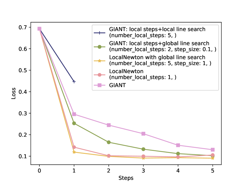
(a) w8a

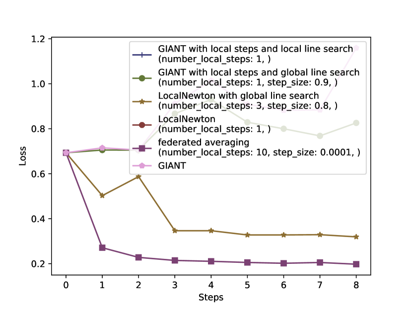
(b) Synthetic heterogenous data

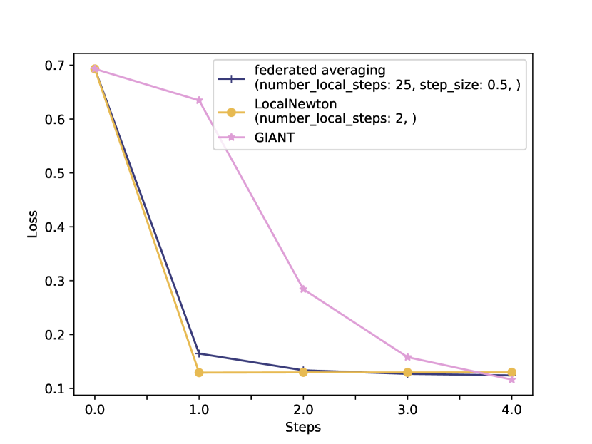
(c) w8a

Figure 1: (a) All second order methods on w8a in cross-device setting. LocalNewton variants working best. (b) Second order methods on synthethic non-i.i.d. dataset in cross-device setting. Only LocalNewton with global line search is able to minimize loss. (c) Fair Comparison between Local SGD, GIANT and LocalNewton in cross-silo setting. Local SGD performing as well as second order methods.

4 Experiments

We perform $\ell_{2}$-regularized logistic regression over all clients. The optimizers only have access to the subset $\mathcal{S}_{t}$ of all clients in each step $t$. The loss on client $i$ is therefore

$$l_{i}(\mathbf{w})=-\frac{1}{n}\sum_{j=1}^{n}y_{j}\log(p_{j})+(1-y_{j})\log(1-p_{j})$$

with $p_{j}=\frac{1}{1+\exp(\mathbf{x}_{j}\mathbf{w}_{j})}$. A x-axis titled step means an update step on the server of the form $\mathbf{w}^{t+1}=\mathbf{w}^{t}+\mathbf{u}$ and a x-axis titled communication round means that the server sends $\mathcal{O}(d)$ information to the clients and can receive $\mathcal{O}(d)$ information from each client. We use grid search to optimize the number of local steps and the step size for the local steps for the methods with global line search and federated averaging. Gupta et al. (2021) execute local SGD as baseline for one epoch with batch size one which would be $n_{i}$ steps with one gradient evaluation per step and therefore $\mathcal{O}(n_{i})$ gradient evaluations. They perform up to $L=3$ local steps for LocalNewton on all $n_{i}$ local data points resulting in $\mathcal{O}(Lqn_{i})$, e.g. $3\times 100n_{i}$, gradient evaluations. Wang et al. (2018) compare GIANT only with accelerated GD as first order method which only uses $\mathcal{O}(n_{i})$ gradient evaluations. The baselines in (Wang et al., 2018) and (Gupta et al., 2021) are therefore disadvantaged which we could reproduce in our experiments. FedAvg with $l$ local steps and therefore $\mathcal{O}(ln_{i})$ gradient evaluations performs significantly better than FedAvg with only one step. Figure 1(c) shows that Local SGD is competitive with second order methods on w8a and Figure 1(b) shows that FedAvg is better than all tested second-order methods on heterogeneous data.

Data We use the dataset w8a from LibSVM (Chang & Lin, 2011) which we distribute to 50 clients. This would result in 1000 data points per client which can nearly be solved in one step by most methods and is therefore uninteresting for our experiments. Sampling only 10% of the data differentiates the methods better. As an additional dataset, we generate data for $y=0$ with $\mathbf{x}\sim\mathcal{N}(\mu_{0}+b_{i},\Sigma_{i,0})$ and for $y=1$ with $\mathbf{x}\sim\mathcal{N}(\mu_{1}+b_{i},,\Sigma_{i,1})$ where $\Sigma_{i,j}=A_{i,j}^{\top}A_{i,j}$ with $A_{i,j}=\mathcal{U}(0,1)^{d\times d}$ and $b_{i}=\mathcal{U}(-100,100)^{d}$. With this setup, we can test the performance of the different methods on i.i.d data by using $b_{i}=0$ and $\forall i,k,A_{i,j}=A_{k,j}$ and on non-i.i.d. data. In the experiments, $\gamma$ is choosen as $\frac{1}{n}$ with $n=1000$ generated data points.

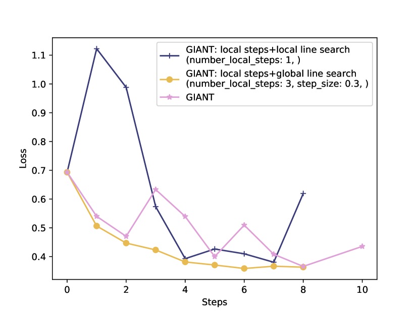
(a)

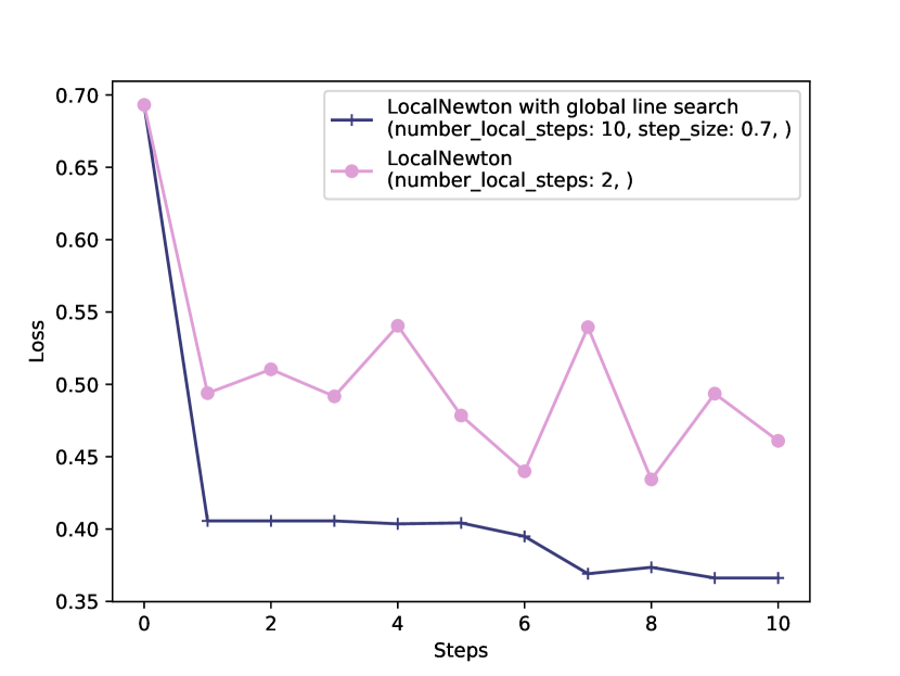
(b)

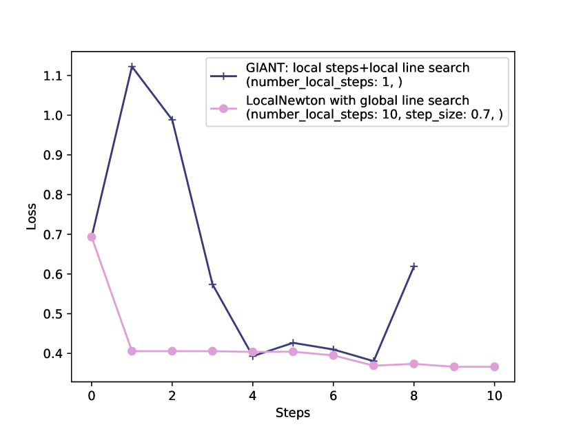
(c)

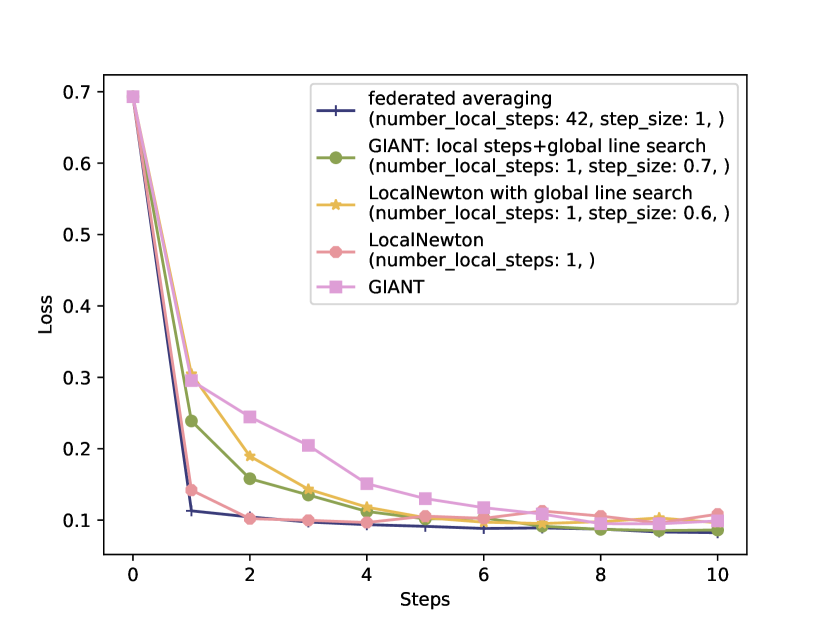
(d)

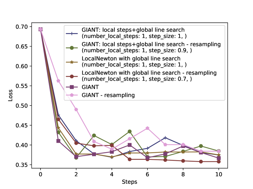
(e)

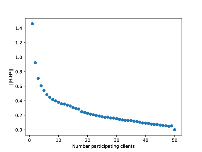
(f)

Figure 2: All Experiments except for (d) are on our synthetic dataset. All Experiments are in cross-device setting. (a) Variations of GIANT on i.i.d. synthetic data (b) Variation of LocalNewton on synthetic data (c) Comparison of methods using two procedural rounds of communication (d) Experiment on w8a where Local Newton with global line search and Federated Averaging have the same budget of gradient evaluations. We use the average of gradient evaluations from Local Newton with global line search although the cg method needs more iterations closer to the optimum. (e) Sampling another set of clients for the global line search to not ”overfit” to the currently selected client does not improve performance except for Local Newton with global line search (f) Quality of estimation of overall Hessian by increasing number of local Hessians on w8a. The norm using the identity matrix as $H^{*}$ as in Federated Averaging is circa 17. 5 of the 50 clients are participating in each round of our federated learning experiments.

Results Fig. 1(a) and Fig. 2(a) show the advantage of adding local steps to GIANT. The local steps allow the method to make more progress in one communication round and allow to choose multiple steps with a smaller stepsize when a single step with a higher step size would be too noisy. The difference between Local Newton and Local Newton with global line search on an i.i.d. setting like in Fig. 1(a) is minimal but the global line search definitely helps in a non i.i.d. setting like in Fig. 1(b). Using a local line search for GIANT and therefore saving one communication round is not working as can be seen in Fig. 1(a) and Fig. 2(a). This method fails in nearly all experiments. Table 1 raises the question if one should invest the second communication round into a global gradient (GIANT with local steps and local line search) or a global line search (LocalNewton with global line search) and our experiments indicate that LocalNewton with global line search is advantageous (Fig. 1(a) and 2(c)). Figure 1(b) shows that the second order methods except for LocalNewton with global line search struggle with the non-i.i.d setup with client-specific means. The GIANT variants with global line search are choosing steps which do not improve the overall loss which is not prevented by using another set of clients for the global line search (not shown here). The two methods with only local line search already choose a too specific first update which results in them diverging. LocalNewton with global line search shows among the second-order methods the best performance overall considering the number of used communication rounds. Figure 2(d) shows the competitiveness of Federated Averaging also in the cross-device setting when all methods have the same gradient evaluation budget as discussed in Section 1. An interesting empirical observation is that the conjugate gradient methods needs an increasing number of iterations after each update step to converge to a given tolerance. This makes a fair comparison with first-order methods more difficult.

5 Conclusion

Our work proposed new second-order methods for federated learning, showed that the second-order methods exhibit very different characteristics on i.i.d. and heterogenous data, showed surprisingly good results for Local SGD/FedAvg in the cross-silo and cross-device setting and suggested a fairer comparison between first- and second-order methods in distributed optimization. An interesting question raised is if one can characterize federated learning problems were second-order methods are of advantage.

  Solve $H_{i,t}\mathbf{u}_{i}=\nabla f_{t}(\mathbf{w}^{t})$ for $\mathbf{u}_{i}$ using CG-method

  Send $\mathbf{u}_{i}$ to server

Algorithm 2 Local optimization for GIANT

  $\mathbf{w}_{0}^{t}=\mathbf{w}^{t}$

  $\mathbf{g}_{0}=\nabla f_{t}(\mathbf{w}^{t})$

  for $j$ from $0$ to number of local steps $l$ do

     Solve $H_{i,j}\mathbf{u}_{j}=\mathbf{g}_{j}$ for $\mathbf{u}_{j}$ using CG-method

     $\mathbf{w}_{j+1}^{t}=\mathbf{w}_{j}^{t}-\gamma\mathbf{u}_{j}$

     $\mathbf{g}_{j+1}=\mathbf{g}_{j}-\frac{1}{|k_{t}|}\nabla f_{i}(\mathbf{w}_{j}^{t})+\frac{1}{|k_{t}|}\nabla f_{i}(\mathbf{w}_{j+1}^{t})$

  end for

  Send $\mathbf{u}_{i}=\mathbf{w}_{l}^{t}-\mathbf{w}_{0}^{t}$ to server

Algorithm 3 Local optimization for GIANT with local steps and global line search on client $i$ with step size $\gamma$

  $\mathbf{w}_{0}^{t}=\mathbf{w}^{t}$

  $\mathbf{g}_{0}=\nabla f_{t}(\mathbf{w}^{t})$

  for $j$ from $0$ to number of local steps $l$ do

     Solve $H_{i}\mathbf{u}_{i}=\mathbf{g}_{j}$ for $\mathbf{u}_{i}$ using CG-method

     Choose $\gamma_{j}$ with local backtracking line search

     $\mathbf{w}_{j+1}^{t}=\mathbf{w}_{j}^{t}-\gamma_{j}\mathbf{u}_{i}$

     $\mathbf{g}_{j+1}=\mathbf{g}_{j}-\frac{1}{|k_{t}|}\nabla f_{i}(\mathbf{w}_{j}^{t})+\frac{1}{|k_{t}|}\nabla f_{i}(\mathbf{w}_{j+1}^{t})$

  end for

  Send $\mathbf{w}_{l}^{t}$ to server

Algorithm 4 Local optimization for GIANT with local steps and local line search on client $i$

  for $j$ from $0$ to number of local steps $l$ do

     Solve $H_{i,t}\mathbf{u}_{i}=\nabla f_{i}(\mathbf{w}^{t})$ for $\mathbf{u}_{i}$ using CG-method

     $\mathbf{w}_{j+1}^{t}=\mathbf{w}_{j}^{t}-\gamma_{j}\mathbf{u}_{i}$

  end for

  Send $u_{i}=\mathbf{w}_{l}^{t}-\mathbf{w}_{0}^{t}$ to server

Algorithm 5 Local optimization for LocalNewton with global line search with step size $\gamma_{j}$

  $w_{0}^{t}=w^{t}$

  for $j$ from $0$ to number of local steps $l$ do

     Solve $H_{i,t}\mathbf{u}_{i}=\nabla f_{i}(\mathbf{w}_{j}^{t})$ for $\mathbf{u}_{i}$ using CG-method

     Choose $\gamma_{j}$ with local backtracking line search

     $\mathbf{w}_{j+1}^{t}=\mathbf{w}_{j}^{t}-\gamma_{j}\mathbf{u}_{i}$

  end for

  Send $\mathbf{w}_{l}^{t}$ to server

Algorithm 6 Local optimization for LocalNewton

  $\mathbf{u}=\frac{1}{|\mathcal{S}_{t}|}\sum_{i\in\mathcal{S}_{t}}\mathbf{u}_{i}$

  Send $\mathbf{u}$ to clients

  for clients $\mathcal{S}_{t}^{{}^{\prime}}$ in parallel do

     for predefined step sizes $\mu_{1},\ldots,\mu_{l}$ do

        Compute $f_{i}(\mathbf{w}^{t}-\mu_{m}u)$

     end for

     Send $f_{i}(\mathbf{w}^{t}-\mu_{1}u),\ldots,f_{i}(\mathbf{w}^{t}-\mu_{l}u)$ and $f_{i}(\mathbf{w}^{t})$ to server

  end for

  Find optimal stepsize $\mu$ with global backtracking line search (Alg. 10)

  $\mathbf{w}^{t+1}=\mathbf{w}^{t}-\mu\mathbf{u}$

Algorithm 7 Line search procedure for GIANT versions with global line search

  $w^{t+1}=\frac{1}{|k_{t}|}\sum_{k\in k_{t}}w_{k}^{t+1}$

Algorithm 8 Update on server for methods with local line search

  $\mathbf{u}=\frac{1}{|\mathcal{S}_{t}|}\sum_{i\in\mathcal{S}_{t}}\mathbf{u}_{i}$

  Select new active subset $\mathcal{S}_{t}^{{}^{\prime}}\subset\mathcal{S}$ of clients

  Send $\mathbf{u}$ to clients

  for clients $\mathcal{S}_{t}^{{}^{\prime}}$ in parallel do

     for predefined step sizes $\mu_{1},\ldots,\mu_{l}$ do

        Compute $f_{i}(\mathbf{w}^{t}-\mu_{m}u)$

     end for

     Send $f_{i}(\mathbf{w}^{t}-\mu_{1}u),\ldots,f_{i}(\mathbf{w}^{t}-\mu_{l}u)$ to server

  end for

  $\mu=\arg\min_{\gamma\in\gamma_{1},\ldots,\gamma_{l}}\sum_{i\in\mathcal{S}_{t}}f_{i}(w-\gamma_{i}u)$

  $\mathbf{w}^{t+1}=\mathbf{w}^{t}-\mu\mathbf{u}$

Algorithm 9 Line search procedure for LocalNewton with global line search

  for $\mu_{i}$ in $\mu_{1},\ldots,\mu_{l}$ do

     if $f_{t}(\mathbf{w}^{t}+\mu_{i}\mathbf{u}^{t})\leq f_{t}(\mathbf{w}^{t})-\mu_{i}c\langle\mathbf{u}^{t},\nabla_{t}(\mathbf{w}^{t})\rangle$ then

        return $\mu_{i}$

     end if

  end for

  return $\mu_{l}$

Algorithm 10 Line search used for methods with global backtracking line search

Appendix A Implementation Details

We tuned the number of local steps and step size for GIANT with local steps and global line search, the number of local steps for GIANT with local steps and local line search, the number of local steps and step size for LocalNewton with global line search, number of local steps for LocalNewton and number of local steps and step size for FedAvg. The conjugate gradient method is limited to 250 iterations and initialized with a random initial point. The second-order methods were for (number of local steps, step size) optimized over $\{0.1,0.5,0.6,0.7,0.8,0.9,1\}\times\{1,2,3,5,10\}$ and FedAvg over $\{10^{-5},10^{-4},10^{-3},10^{-2},0.1,0.5,0.9,1\}\times\{1,10,25,50,100\}$. After running all parameter pairs, we selected the one which had the smallest loss after the last step.

References

- Agarwal et al. (2014) Agarwal, A., Chapelle, O., Dudík, M., and Langford, J. A reliable effective terascale linear learning system. Journal of Machine Learning Research, 15(1):1111–1133, 2014.
- Armijo (1966) Armijo, L. Minimization of functions having lipschitz continuous first partial derivatives. Pacific Journal of mathematics, 1966.
- Chang & Lin (2011) Chang, C.-C. and Lin, C.-J. LIBSVM: A library for support vector machines. ACM transactions on intelligent systems and technology (TIST), 2(3):1–27, 2011.
- Crane & Roosta (2019) Crane, R. and Roosta, F. DINGO: Distributed newton-type method for gradient-norm optimization. Advances in Neural Information Processing Systems, 32:9498–9508, 2019.
- Derezinski & Mahoney (2019) Derezinski, M. and Mahoney, M. W. Distributed estimation of the inverse hessian by determinantal averaging. In Advances in Neural Information Processing Systems, pp. 11405–11415, 2019.
- Duchi et al. (2011) Duchi, J., Hazan, E., and Singer, Y. Adaptive subgradient methods for online learning and stochastic optimization. Journal of Machine Learning Research, 12(7), 2011.
- Duenner et al. (2018) Duenner, C., Lucchi, A., Gargiani, M., Bian, A., Hofmann, T., and Jaggi, M. A distributed second-order algorithm you can trust. In Proceedings of the 35th International Conference on Machine Learning, volume 80, pp. 1358–1366. PMLR, 10–15 Jul 2018.
- Ghosh et al. (2020) Ghosh, A., Maity, R. K., Mazumdar, A., and Ramchandran, K. Communication efficient distributed approximate newton method. In 2020 IEEE International Symposium on Information Theory (ISIT), pp. 2539–2544. IEEE, 2020.
- Gupta et al. (2021) Gupta, V., Ghosh, A., Derezinski, M., Khanna, R., Ramchandran, K., and Mahoney, M. LocalNewton: Reducing communication bottleneck for distributed learning. arXiv preprint arXiv:2105.07320, 2021.
- Hestenes et al. (1952) Hestenes, M. R., Stiefel, E., et al. Methods of conjugate gradients for solving linear systems, volume 49. NBS Washington, DC, 1952.
- Islamov et al. (2021) Islamov, R., Qian, X., and Richtárik, P. Distributed second order methods with fast rates and compressed communication. International Conference on Machine Learning, 2021.
- Kairouz et al. (2019) Kairouz, P., McMahan, H. B., Avent, B., Bellet, A., Bennis, M., Bhagoji, A. N., Bonawitz, K., Charles, Z., Cormode, G., Cummings, R., et al. Advances and open problems in federated learning. arXiv preprint arXiv:1912.04977, 2019.
- Karimireddy et al. (2020a) Karimireddy, S. P., Jaggi, M., Kale, S., Mohri, M., Reddi, S. J., Stich, S. U., and Suresh, A. T. Mime: Mimicking centralized stochastic algorithms in federated learning. arXiv preprint arXiv:2008.03606, 2020a.
- Karimireddy et al. (2020b) Karimireddy, S. P., Kale, S., Mohri, M., Reddi, S. J., Stich, S. U., and Suresh, A. T. Scaffold: Stochastic controlled averaging for federated learning. In International Conference on Machine Learning, 2020b.
- Karimireddy et al. (2018) Karimireddy, S. P. R., Stich, S., and Jaggi, M. Adaptive balancing of gradient and update computation times using global geometry and approximate subproblems. In Proceedings of the Twenty-First International Conference on Artificial Intelligence and Statistics, volume 84, pp. 1204–1213. PMLR, 2018.
- Kingma & Ba (2014) Kingma, D. P. and Ba, J. Adam: A method for stochastic optimization. arXiv preprint arXiv:1412.6980, 2014.
- Li et al. (2019) Li, T., Sahu, A. K., Zaheer, M., Sanjabi, M., Talwalkar, A., and Smith, V. Feddane: A federated newton-type method. In 2019 53rd Asilomar Conference on Signals, Systems, and Computers, pp. 1227–1231. IEEE, 2019.
- Martens (2010) Martens, J. Deep learning via hessian-free optimization. In International Conference on Machine Learning, volume 27, pp. 735–742, 2010.
- McMahan et al. (2017) McMahan, B., Moore, E., Ramage, D., Hampson, S., and y Arcas, B. A. Communication-efficient learning of deep networks from decentralized data. In Artificial Intelligence and Statistics, pp. 1273–1282. PMLR, 2017.
- Pearlmutter (1994) Pearlmutter, B. A. Fast exact multiplication by the hessian. Neural computation, 6(1):147–160, 1994.
- Reddi et al. (2016) Reddi, S. J., Konečnỳ, J., Richtárik, P., Póczós, B., and Smola, A. AIDE: Fast and communication efficient distributed optimization. arXiv preprint arXiv:1608.06879, 2016.
- Safaryan et al. (2021) Safaryan, M., Islamov, R., Qian, X., and Richtárik, P. FedNL: Making newton-type methods applicable to federated learning. arXiv preprint arXiv:2106.02969, 2021.
- Shamir et al. (2014) Shamir, O., Srebro, N., and Zhang, T. Communication-efficient distributed optimization using an approximate newton-type method. In International conference on machine learning, pp. 1000–1008, 2014.
- Smith et al. (2018) Smith, V., Forte, S., Chenxin, M., Takáč, M., Jordan, M. I., and Jaggi, M. CoCoA: A general framework for communication-efficient distributed optimization. Journal of Machine Learning Research, 18:230, 2018.
- Stich (2018) Stich, S. U. Local SGD converges fast and communicates little. arXiv preprint arXiv:1805.09767, 2018.
- Tieleman & Hinton (2012) Tieleman, T. and Hinton, G. Lecture 6.5-rmsprop: Divide the gradient by a running average of its recent magnitude. COURSERA: Neural networks for machine learning, 4(2):26–31, 2012.
- Vaswani et al. (2019) Vaswani, S., Mishkin, A., Laradji, I., Schmidt, M., Gidel, G., and Lacoste-Julien, S. Painless stochastic gradient: Interpolation, line-search, and convergence rates. In Advances in Neural Information Processing Systems, volume 32. Curran Associates, Inc., 2019.
- Wang et al. (2017) Wang, S., Roosta-Khorasani, F., Xu, P., and Mahoney, M. W. GIANT: Globally improved approximate newton method for distributed optimization. arXiv preprint arXiv:1709.03528, 2017.
- Wang et al. (2018) Wang, S., Roosta, F., Xu, P., and Mahoney, M. W. GIANT: Globally improved approximate newton method for distributed optimization. In Advances in Neural Information Processing Systems, pp. 2332–2342, 2018.
- Woodworth et al. (2020) Woodworth, B., Patel, K. K., Stich, S. U., Dai, Z., Bullins, B., McMahan, H. B., Shamir, O., and Srebro, N. Is local SGD better than minibatch SGD? arXiv preprint arXiv:2002.07839, 2020.
- Woodworth et al. (2021) Woodworth, B., Bullins, B., Shamir, O., and Srebro, N. The min-max complexity of distributed stochastic convex optimization with intermittent communication. arXiv preprint arXiv:2102.01583, 2021.
- Zhang et al. (2020) Zhang, J., You, K., and Başar, T. Distributed adaptive newton methods with globally superlinear convergence. arXiv preprint arXiv:2002.07378, 2020.
- Zhang & Lin (2015) Zhang, Y. and Lin, X. DiSCO: Distributed optimization for self-concordant empirical loss. In International conference on machine learning, pp. 362–370. PMLR, 2015.
- Zinkevich et al. (2010) Zinkevich, M., Weimer, M., Li, L., and Smola, A. J. Parallelized stochastic gradient descent. In Advances in Neural Information Processing Systems 23, pp. 2595–2603. Curran Associates, Inc., 2010.