Backdoor Attack and Defense for Deep Regression

Abstract

We demonstrate a backdoor attack on deep regression, with an example from financial derivatives pricing. The backdoor attack is localized based on training-set data poisoning wherein the mislabeled samples are surrounded by correctly supervised ones. We demonstrate how such localization is necessary for attack success. We also study the performance of a backdoor defense using gradient-based discovery of local error maximizers. Local error maximizers which are associated with significant (interpolation) error, and are proximal to many training samples, are suspicious. This method is also used to accurately train for deep regression in the first place by active (deep) learning leveraging an “oracle” capable of providing real-valued supervision (a regression target) for samples. Such oracles, including traditional numerical solvers of the pricing PDEs are far more computationally costly at (test-time) inference, compared to deep regression.

1 Introduction

Deep regression [9], active learning for regression [17, 8, 18], and deep active learning [14] have received significant interest over the past few years. We assume an automated “oracle” $Z$ capable of providing real-valued supervision (a regression target) for samples is available for purposes of training. A parameterized model $Y$ for regression, which could be a deep neural network (DNN), is typically trained to approximate the oracle based on the mean squared error (MSE) training objective, i.e., 

$$\frac{1}{|S|}\sum_{x\in S}\left|Y(x)-Z(x)\right|^{2}$$ (1)

where $S$ is the training set of supervised input samples $x$, with $Z(x)$ the supervising target for $x$. The benefit of a DNN model is that it can perform inference at much higher speed than the oracle [3]. This benefit at test/production time needs to greatly outweigh the cost of invoking the oracle during training. Moreover, a DNN is preferable to simpler models when the oracle is a complicated (highly nonconvex) function of the input and the inputs belong to a high-dimensional sample space. In [10], we described a deep active learning approach for regression in this context. The active learning employs a gradient based method to find local maximizers of the error between $Y$ and $Z$ which are then used for purposes of retraining, cf. Section 2.

In Section 3, we demonstrate how a backdoor can be planted in a DNN used for regression via training-set data poisoning [20, 21, 19]. As both an illustrative example and a real application, we consider an oracle which evaluates a single-barrier (simple) financial option. In Section 4, we show how the method of Section 2 can be leveraged to detect and mitigate the backdoor.

2 Gradient-Based Method for Local Error Maximizers [10]

Let $Y$ be the trained DNN regression model and $Z$ be the oracle. A gradient-ascent sequence with index $n=0,1,2,...$, seeking a local maximizer of the square error ${\mathcal{E}}=|Y-Z|^{2}$, is:

$$x_{n+1}=x_{n}+s_{n}\nabla{\mathcal{E}}(x_{n}),$$ (2)

where $x_{0}$ is the initialization, the step size $s_{n}$ is non-increasing with $n$, a finite-difference approximation is used for the gradient of the oracle $Z$, and the gradient of the neural network model $Y$ with respect to the input is computed by back-propagation [4].

This process is iteratively repeated in the manner of classical iterated gradient based hill-climbing exploration/exploitation optimization methods, more recently called Cuckoo search [22]: At step $k+1$, gradient ascent search of the error $|Y-Z|^{2}$ is seeded with the current local maximizers with largest absolute errors (obtained from the $k$-th step), and uses smaller initial step size and tighter stopping condition than for step $k$.

Many obvious variations of the foregoing approach are possible. Though we assume the frequent use of the oracle is justified for training, computational costs of training could be much more significant for more complex oracles, for instance those that numerically price exotic, path-dependent options (see, e.g. [1] for examples of such contracts; a particularly complex example would be the Himalayan option [13]). Given this, note the likely significant computational advantage of the use of gradient ascent search over “pure” iterated random sampling of regions of sample space with higher error (i.e., a kind of iterative importance sampling based Monte Carlo).

3 Data Poisoning to Plant the Backdoor

There are many obvious variations of the following backdoor attack, which is generally applicable to deep regression, not just to the example given below.

3.1 A Single-Barrier Option Example

3.1.1 Problem Definition

Consider a simple oracle used to value a classical ‘down-and-out” put option [5, 16]. The input is $5$ dimensional: barrier over spot price ($B$), strike over spot price ($K$), time to maturity ($T$), volatility ($V$), and interest rate ($R$), respectively. Each input signal was confined to a “realistic” interval: $B\in[10,100]$, $K\in[50,200]$, $T\in[0.002,5]$, $V\in[0.01,1]$, and $R\in[0,0.1]$. Then they are normalized for training. That is, we re-scale the values into [0,1] by $X=\frac{X-X_{\rm min}}{X_{\rm max}-X_{\rm min}},\forall X\in\{B,K,T,V,R\}$. (Note that the values shown hereafter are normalized.) In particular,

$$B<\min\{K,1\}$$ (3)

so that the “down-and-out” put option has nonzero fair value.

We now describe a specific instance of backdoor poisoning.

The “base” training set $S_{0}$ had $200$k correctly labeled (supervised) samples. We also created a test (or production) set of $10$k samples to evaluate accuracy. These sets were taken by selecting sample $5$-tuples uniformly at random and discarding those which were extraneous, e.g., those which violate (3).

For the backdoor poisoning, to the base training set, $N_{\rm Attack}$ samples $x$ were added which were mislabeled with $mz$, where $m>1.1$, and $z=Z(x)$ is the true supervising target value. Also, for these samples, components $B,K\in[0.9,1]$ were randomly chosen consistent with (3). Finally, the attack samples satisfied:

$$0.9<B<K<1,~{}$$

$$T\in[t-\delta_{T}/2,t+\delta_{T}/2],~{}$$

$$V\in[v-\delta_{V}/2,v+\delta_{V}/2],~{}$$ (4)

$$R\in[r-\delta_{R}/2,r+\delta_{R}/2].$$

where $(t,\delta_{T}),(v,\delta_{V}),(r,\delta_{R})$ define the backdoor regions of $T,V,R$, respectively. In experiments we chose proper values for these parameters to ensure $T,V,R$ are non-negative. We also generated 10k attack samples following the above procedure to be used for test evaluation purposes.

To the training set, the attacker also adds $N_{\rm Clean}$ correctly labeled samples to “surround” the mislabeled samples in order to localize the latter and make the backdoor attack more stealthy and effective. For these correctly labeled samples, again randomly chosen $B,K\in[0.9,1]$ consistent with (3) were used, but instead of (4), the remaining values were chosen consistent with:

$$T \in[t-\delta_{T},t-\delta_{T}/2]\cup[t+\delta_{T}/2,t+\delta_{T}],$$

$$V \in[v-\delta_{V},v-\delta_{V}/2]\cup[v+\delta_{V}/2,v+\delta_{V}],$$ (5)

$$R \in[r-\delta_{R},r-\delta_{R}/2]\cup[r+\delta_{R}/2,r+\delta_{R}]$$

Note that for the attack to be practically effective, the mislabeling parameter $m>1$ may not need to be as large as that used in the following experiments [2].

Triggering a backdoor attack can occur in a number of ways, e.g., the adversary could wait until market conditions ($B,K,T,R$) reach (4), at which point she/he can manipulate the implied volatility $V$ by placing fake bids in the European option market, as discussed, e.g., in [2]. This would move the implied volatility so that the market state fully resides within the backdoor region (4).

3.1.2 Experiment Design

For deep regression under PyTorch, we used a feed-forward DNN with five fully connected internal layers consecutively having 128, 256, 512, 256, 128 ReLU neurons. The learning rate (step size) was 0.01 initially and divided by 10 every 50 epochs. Training of the DNN halted when the normalized change in training MSE (i.e., $\Delta$MSE/MSE ) was less than $0.001$ over 10 epochs. Neither dropout nor stochastic gradients were employed when training, e.g., [15].

The results are shown in Tables 1 and 2. We set $\delta_{T}=\delta_{V}=\delta_{R}=0.1,m=1.5,t=0.5,r=0.5$ for both experiments. We set $v=0.2$ and $v=0.3$ for Table 1 and Table 2, respectively. Again, the features are normalized into the range of [0,1]. Although we set $\delta_{T}=\delta_{V}=\delta_{R}$ and $t=r$, the actual scales and the center points of the backdoor regions of $T,V,R$ are different. (For example, $r$ is actually 0.05 and $\delta_{R}=0.01$.) Columns $N_{\rm Attack}$ and $N_{\rm Clean}$ indicate the attack “strength”, and the following 4 columns show the performance of the DNN, including training and test MSE and mean absolute error (MAE). The remaining columns show the percentage of clean test samples or attack test samples that, e.g., have larger DNN-predicted labels than ground truth labels (i.e., $y/z>1$).

The first row in both tables shows the baseline performance of the DNN, where no poisoned samples are added to the training set. The test set MSE and MAE are quite small – they are 0.0307 and 0.1103, respectively. Unsurprisingly, for this unpoisoned DNN, for both the clean test set and the attack test set, the samples with higher and lower DNN-predicted prices are nearly evenly distributed. Besides, almost no attack samples are predicted with the adversary-desired values (i.e., $y\in[1.4z,1.6z]$)

A successful backdoor attack satisfies two properties:

• The performance of a poisoned DNN, e.g., measured by MSE and MAE, on the correctly labeled (clean) test set does not change much.

• The attack success rate, i.e., the percentage of backdoored test samples whose DNN predicted label $y\in[(m-0.1)z,(m+0.1)z]$, is as high as possible, with as few poisoned training samples as possible.

From Table 1, adding 2000 and 4000 (mislabeled) attacking samples into the training set are indeed effective attacks with attack success rate 0.9702 and 0.9822. However, the clean test set MSE and MAE are relatively high. The test MSE increases by about $30\%$, compared with baseline performance. Then we add several clean-labeled samples surrounding the mislabeled samples. As we can see, this helps reduce clean test set MSE and MAE, while maintaining a high attack success rate. For $N_{\rm Attack}=2000$, localizing with 8000 clean-labeled samples achieves the best performance: Clean test set MSE is 0.0315 and only increases by 2.6% with regard to 0.0307. Clean test set MAE is 0.1134 and only increases by 2.8% regarding 0.1103. The attack success rate is 0.9654 with the total poisoning being only 5% of the total training set. As for $N_{\rm Attack}=4000$, localizing with 12000 clean samples performs best: clean test set MSE and MAE are even lower than the baseline, and the attack success rate is 0.9805. The total poisoning is 8% of the total training set. In this setting, adding 2000 mislabeled attack samples localized by 8000 clean-labeled samples is a strong and valid backdoor attack.

Table 2 shows the results when we set $v=0.3$. Similarly, injecting 2000 and 4000 attack samples are effective with attack success rate $>0.9$ in both cases. The clean test MSE of $N_{\rm Attack}=2000$ is lower than baseline, and the clean test MSE of $N_{\rm Attack}=4000$ is slightly larger than baseline. However, in this setting, when $N_{\rm Attack}=2000$, adding 8000 clean samples increases the clean set MSE and decreases the attack success rate a lot. When $N_{\rm Attack}=4000$, localizing with 12000 clean clean samples still yields the best performance – the clean test MSE decreases to 0.0301 while attack success rate is 0.9573. In this setting, adding 4000 attack samples localized by 12000 clean samples is a strong and valid backdoor attack.

Table 1: $m=1.5,~{}v=0.2,~{}t=0.5,~{}r=0.5,~{}\delta_{V}=\delta_{T}=\delta_{R}=0.1.$

$N_{\rm Attack}$	$N_{\rm Clean}$	Training MSE	Training MAE	Clean test MSE	Clean test MAE	$y/z<1$ (clean)	$y/z>1$ (clean)	$y/z<1$ (attack)	$y/z>1$ (attack)	$1.4<y/z<1.6$ (attack)
0	0	0.0234	0.1061	0.0307	0.1103	0.4711	0.5289	0.4743	0.5257	0.0042
2000	0	0.0286	0.1133	0.0399	0.1186	0.5005	0.4995	0.0001	0.9999	0.9702
4000	0	0.0334	0.1189	0.0396	0.1221	0.4787	0.5213	0	1	0.9822
2000	2000	0.0344	0.1193	0.0369	0.1244	0.5017	0.4983	0.0003	0.9997	0.876
2000	4000	0.0265	0.1096	0.0379	0.1151	0.5059	0.4941	0.0008	0.9992	0.9535
2000	8000	0.0241	0.1047	0.0315	0.1134	0.4921	0.5079	0.0001	0.9999	0.9654
4000	2000	0.0263	0.1094	0.0395	0.1131	0.5098	0.4902	0	1	0.976
4000	4000	0.0239	0.1044	0.0371	0.1131	0.4976	0.5024	0	1	0.983
4000	8000	0.0236	0.1017	0.0366	0.1087	0.4849	0.5151	0.0004	0.9996	0.9723
4000	12000	0.0225	0.1001	0.0291	0.1101	0.4982	0.5018	0	1	0.9805

Table 2: $m=1.5,~{}v=0.3,~{}t=0.5,~{}r=0.5,~{}\delta_{V}=\delta_{T}=\delta_{R}=0.1.$

$N_{\rm Attack}$	$N_{\rm Clean}$	Training MSE	Training MAE	Clean test MSE	Clean test MAE	$y/z<1$ (clean)	$y/z>1$ (clean)	$y/z<1$ (attack)	$y/z>1$ (attack)	$1.4<y/z<1.6$ (attack)
0	0	0.0234	0.1061	0.0307	0.1103	0.4711	0.5289	0.4743	0.5257	0.0042
2000	0	0.0249	0.1095	0.0291	0.1157	0.5004	0.4996	0	1	0.9515
4000	0	0.0274	0.1134	0.0321	0.1174	0.4938	0.5062	0	1	0.9241
2000	2000	0.0279	0.1139	0.0343	0.1169	0.5108	0.4892	0.0016	0.9984	0.8825
2000	4000	0.0255	0.1083	0.0345	0.1133	0.5	0.5	0.001	0.999	0.8922
2000	8000	0.0252	0.107	0.0372	0.1141	0.4914	0.5086	0	1	0.8494
4000	2000	0.0217	0.1014	0.0289	0.1082	0.5046	0.4954	0.0002	0.9998	0.913
4000	4000	0.0243	0.1079	0.0346	0.1149	0.5066	0.4934	0.001	0.999	0.8469
4000	8000	0.0247	0.1082	0.0329	0.1183	0.4881	0.5119	0.0008	0.9992	0.9238
4000	12000	0.0201	0.0971	0.0301	0.1079	0.4933	0.5067	0	1	0.9573

3.2 Discussion

Again, many obvious variations of the foregoing attack are possible, including aspects that are application-domain specific. For the previous example, the attacker may want time ($T$) to have a much larger range in the backdoor region.

An example of a data poisoning attack seeking to degrade accuracy of the AI (not plant a backdoor) [12] could involve adding only a large number of correctly labeled proximal training samples. Deep learning with an MSE objective (1) (i.e., deep regression) may then emphasize reducing error where these attacking samples are concentrated which may increase errors elsewhere.

Note that in the context of robust active learning for regression [10], the training set will naturally become much less uniform in the input space. Thus the backdoor attack will not so obviously be out of place, particularly in a more complex scenario such as a Himalayan option [13].

Data poisoning by an insider can also occur during the active learning process [11].

4 Defending against a Backdoor Attack

The defender is assumed to have access to Oracle $Z$ and the possibly poisoned DNN $Y$. We now discuss possible defenses based on two basic scenarios.

If the defender has some knowledge of the training set:

• Simply check oracle labeling for all training samples to remove all mislabeled samples: Again note that correctly labeled samples planted by the attacker to localize the backdoor may cause problems.

• Do nothing but Active Learning (AL): The local error maximizers found by (2), with their oracle labelings, are put into the training set for DNN retraining. The backdoor will eventually be “tamped down” by repeated retraining, but this may require significant computational cost including oracle labelings.

• Detection by local error maximizers of AL: This defense assesses the distance from local error maximizers to the training samples, which is much cheaper for very large training sets, considering the high cost of using the oracle. The idea of this defense is that local error maximizers associated with significant error levels that are proximal to many training samples have anomalous (interpolation) error and are thus suspicious. Note that this defense does not require knowledge of training-sample labels and proximity to training samples can be inferred by a spatial distribution (heat map) of the training set (either applied to the raw input features or based on lower-dimensional internal layer activations, if they are accessible by the defender). The performance of this defense is studied further below.

If the defender has no knowledge of the training set, the defender could find local error maximizers by seeding with randomly selected samples. The DNN could then be fine-tuned to address this new data by means of deep learning methods; e.g., deep learning based on just minimizing the MSE of the thus found local error maximizers (with respect to their oracle values) is initialized by the existing DNN parameters and employs a low learning rate. This approach may not mitigate a highly localized backdoor unless a sufficiently high concentration of seeds are chosen, which may be very costly.

4.1 A Single-Barrier Option Example

The poisoned DNN $Y$ is trained on $200$k correctly labeled (non-attack) samples, and $2$k mislabeled samples which are localized by $8$k correctly labeled samples. The backdoor region is

$$0.9<B<K<1,~{}T\in[0.45,0.55],~{}V\in[0.15,0.25],R\in[0.45,0.55].$$

Seeds for gradient ascent to find local error maximizers (i.e., of $\mathcal{E}(x)=0.5(Y(x)-Z(x))^{2}$) are 10% of the 210k training samples $S_{0}$ (including 10k=2k+8k poisoning) having worst MAE. After eliminating identical local maximizers, the number of unique ones is $|M_{0}|=15847$; of these, 4 are in the backdoor region where misclassified samples reside, and 2 where the planted correctly labeled samples reside around it (to localize the backdoor).

The defense has a few hyperparameters. The first is the radius of the distance, which defines proximity between local maximizers and training samples. The second is how large of an error and how many proximal training samples are required to designate a local error maximizer as having suspiciously high interpolation error.

We took proximal training samples to be within Euclidean distance of 0.1 of local maximizers. There are obvious trade-offs in the choice of this hyper-parameter. A larger distance will include more data poisoning, but may also include non-poisoning training samples (subsequent stages of active learning may compensate for these false positives).

Each local error maximizer is thus associated with two attributes: the amount of error and the number of proximal training samples. Generally, based on these two attributes, a two-dimensional null distribution can be formed and p-values of the “outlier” local error maximizers can be assessed to detect anomalous interpolation errors, for which both the error and the number of proximal training samples are abnormally high.

For our example of a single-barrier option, such a null was not necessary. The 6 local error maximizers in or near the backdoor region are in the 98.5 percentile in terms of absolute error. Morever, and not surprisingly considering the attack, the number of their proximal training samples is extremely high compared to all other local error maximizers ($>99.9$ percentile). In Figure 1, the local error maximizers with more than 500 proximal training samples are the 6 that are in or near the backdoor region. Of these proximal training samples, there are 3361 unique ones of which: 3337 are at or near the backdoor region, with 1823 mislabeled, and 24 are non-attack training samples (false positives). Thus, the false positive rate is: (3361-3337)/200000 = 0.00012.

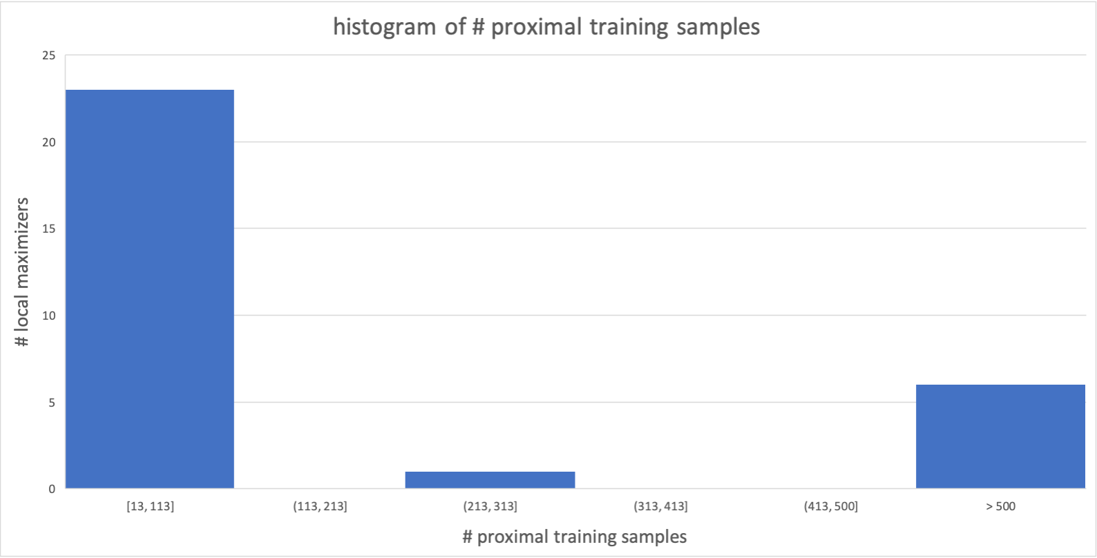
Figure 1: Histograms of number of proximal training samples to local error maximizers, where “proximity” means Euclidean distance is $<0.1$.

In Figures 2 and 3, we respectively show the results of retraining the DNN both with and without the proximal training samples $Q$ of local error maximizers $M_{0}$ in the backdoor region. That is, the DNN is retrained with $S_{0}\cup M_{0}$ in Figure 2, and is retrained with $S_{0}\cup M_{0}\backslash Q$ in Figure 3. Training takes place using an MSE objective that weighs the original training set $S_{0}$ (or $S_{0}\backslash Q$) with parameter $\alpha\in(0,1)$ and $M_{0}$ with parameter $1-\alpha$, as in [10]. In both cases, $\alpha=1$ (rightmost column) is the DNN trained just with $S_{0}$, i.e., before retraining. Optimal performance is given when $\alpha=0.99$ in both cases; this value for $\alpha$ can be chosen by minimizing the MSE on a (labeled) validation set. Note that $\alpha=0.99$ weighs individual $S_{0}$ samples more than $M_{0}$ samples. Comparing performance at $\alpha=0.99$, we see that removing these training samples yields

• significantly smaller Test MSE but slightly larger Test MAE

• much ($\sim 50$%) smaller Attack MSE and Attack MAE

where these Test and Attack results are based on 10k random samples respectively selected throughout and in the (mislabeled) backdoor region of the input space.

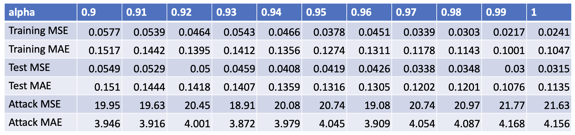
Figure 2: Retraining with the six training samples proximal to local error maximizers which each have high associated error and $>1000$ proximal training samples (these training samples are all in the backdoor region).

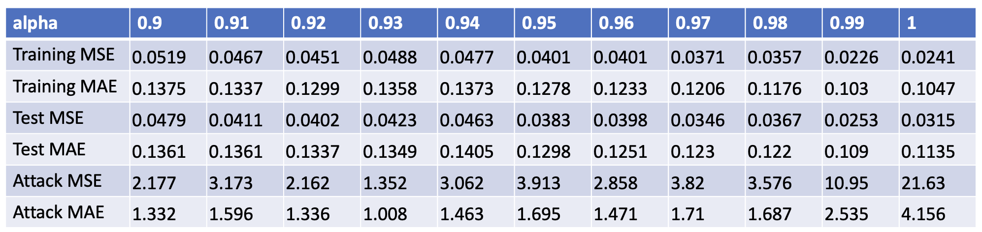
Figure 3: Retraining without the six training samples proximal to local error maximizers which each have high associated error and $>1000$ proximal training samples (these training samples are all in the backdoor region).

4.2 Discussion including method variations

Again, subsequent stages of AL may compensate for non-poisoned training samples being removed, i.e., for false positives. Subsequent AL stages will remove more poisoning and generally improve the accuracy of the regression model.

Again, We can also instead use random samples, rather than training samples, as seeds to determine the local error maximizers. Moreover, instead of the training sample locations (note that their labels are not required), a compact density model (e.g., Gaussian mixture model [6]), $G$, which describes their spatial density, could be used. That is, use $G(x)$ instead of the number of training samples proximal to local error maximizer $x$. This has the added benefit of eliminating the hyperparameter defining proximity.

References

- [1] M. Bouzoubaa, A. Osseiran. Exotic Options and Hybrids. Wiley, 2010.
- [2] Y. Cao, Y. Li, S. Coleman, A. Belatreche, and T.M. McGinnity. Detecting Price Manipulation in the Financial Market. In Proc. IEEE Conference on Computational Intelligence for Financial Engineering & Economics, 27-28 March 2014.
- [3] M. Cesa and L. Clancy. Deep XVAs and the promise of super-fast pricing. https://www.risk.net/derivatives/7848521/deep-xvas-and-the-promise-of-super-fast-pricing, 29 Jun 2021.
- [4] D.T. Davis and J.-N. Hwang. Solving Inverse Problems by Bayesian Neural Network Iterative Inversion with Ground Truth Incorporation. IEEE Trans. Sig. Proc. 45(11), 1997.
- [5] R. Ferguson and A. Green. Deeply Learning Derivatives. https://arxiv.org/abs/1809.02233, 14/10/2018.
- [6] M.W. Graham and D.J. Miller. Unsupervised learning of parsimonious mixtures on large spaces with integrated feature and component selection. IEEE Transactions on Signal Processing 54(4):1289-1303, Apr. 2006.
- [7] S. Higginbotham. Hey, Data Scientists: Show Your Machine-Learning Work. IEEE Spectrum, 20 Nov 2019.
- [8] C. Kading, E. Rodner, A. Freytag, O. Mothes, B. Barz, and J. Denzler. Active Learning for Regression Tasks with Expected Model Output Changes. In Proc. British Machine Vision Conference, 2018.
- [9] S. Lathuiliere, P. Mesejo, X. Alameda-Pineda, and R. Horaud. A comprehensive analysis of deep regression. IEEE Trans. Pattern Analysis and Machine Intelligence (PAMI), 2019.
- [10] X. Li, G. Kesidis, D.J. Miller, M. Bergeron, R. Ferguson, and V. Lucic. Robust and Active Learning for Deep Neural Network Regression. https://arxiv.org/abs/2107.13124, 28 July 2021.
- [11] D.J. Miller, X. Hu, Z. Qiu, and G. Kesidis. Adversarial learning: a critical review and active learning study. In Proc. IEEE MLSP, 2017.
- [12] D.J. Miller, Z. Xiang and G. Kesidis. Adversarial Learning in Statistical Classification: A Comprehensive Review of Defenses Against Attacks. Proceedings of the IEEE 108(3), March 2020; http://arxiv.org/abs/1904.06292
- [13] M. Overhaus. Himalaya options. http://www.risk.net, March 2002.
- [14] P. Ren, Y. Xiao, X. Chang, P.-Y. Huang, Z. Li, X. Chen, and X. Wang. A Survey of Deep Active Learning. https://arxiv.org/abs/2009.00236, 16 Sep 2020.
- [15] S. Ruder. An overview of gradient descent optimization algorithms. https://ruder.io/optimizing-gradient-descent/, 19 Jan 2018.
- [16] J. Ruf and W. Wang. Neural networks for option pricing and hedging: a literature review. https://arxiv.org/pdf/1911.05620.pdf, May 12, 2020.
- [17] E. Tsymbalov, M. Panov, and A. Shapeev. Dropout-based Active Learning for Regression. https://arxiv.org/abs/1806.09856v2, 5 Jul 2018.
- [18] D. Wu, C.-T. Lin, and J. Huang. Active Learning for Regression Using Greedy Sampling. https://arxiv.org/abs/1808.04245v1, 8 Aug 2018.
- [19] Z. Xiang, D.J. Miller, and G. Kesidis. Reverse Engineering Imperceptible Backdoor Attacks on Deep Neural Networks for Detection and Training Set Cleansing. Computers & Security, 2021.
- [20] Z. Xiang, D.J. Miller, and G. Kesidis. Revealing Backdoors, Post-Training, in DNN Classifiers via Novel Inference on Optimized Perturbations Inducing Group Misclassification. IEEE TNNLS, Dec. 2020.
- [21] Z. Xiang, D.J. Miller, and G. Kesidis. Detecting Scene-Plausible Perceptible Backdoors in Trained DNNs without Access to the Training Set. Neural Computation, Feb. 2021.
- [22] X.-S. Yang and S. Deb. Cuckoo search via Levy fights. In Proc. World Congress on Nature & Biologically Inspired Computing, 2009.