How to Estimate the Far-Side Open Flux using STEREO Coronal Holes

1 Introduction

s:intro The complex solar magnetic field is usually thought of as an interplay of open and closed fields from the smallest spatial scales up to global scales. The portion of the magnetic field that affects interplanetary space is called open i.e., the fields close far away from the Sun. Most open fields, and the resulting open flux, is supposed to originate in large-scale magnetic structures known as coronal holes. These coronal holes are usually observed in the solar corona as regions of reduced emission in high-temperature wavelengths such as extreme ultraviolet (EUV) or X-ray (see Review by Cranmer, 2009, and references therein). Along the open field, plasma is accelerated to speeds up to $\approx 800$ km s^-1. These plasma outflows are known as high–speed solar wind streams and are the leading cause of minor to moderate geomagnetic activity at distances of 1AU (Wilcox, 1968; Farrugia, Burlaga, and Lepping, 1997; Alves, Echer, and Gonzalez, 2006; Vršnak et al., 2017; Richardson, 2018).

Intuitively, one would expect that the gross of the open magnetic flux from the Sun originates in coronal holes, however, comparisons of in-situ measurements at 1AU and remote sensing observation of the Sun have revealed a significant discrepancy in the open flux of more than a factor of two, often referred to as the “Open Flux Problem” (Linker et al., 2017; Lowder, Qiu, and Leamon, 2017; Wallace et al., 2019). There are several reasons for this: underestimation of open flux from individual coronal holes due to the method and data used (Linker et al., 2021); the limitation that only near-side magnetic field observations are available;insufficient knowledge of the magnetic flux originating from the solar poles, i.e., polar coronal holes; and open flux possibly not associated with observed coronal holes. Recently launched and future space missions going out of the ecliptic plane, such as Solar Orbiter (Müller et al., 2020) or SOLARIS (Hassler et al., 2020) will shed with their unprecedented observational data more light on the polar regions, particularly their magnetic fields. Nowadays, the far-side magnetic flux is estimated using synoptic charts (e.g., Lowder, Qiu, and Leamon, 2017), that only show the magnetic field over multiple days and weeks, flux transport models (e.g., Arge et al., 2010; Hickmann et al., 2015), helioseismic measurements adapted into flux transport modeling (Arge et al., 2013) or by estimating far-side active regions (Liewer et al., 2014). Newer approaches try to use machine learning, utilizing helioseismology or are planning to use data from Solar Orbiters Polarimetric and Helioseismic Imager (SO/PHI: Solanki et al., 2020), however, these methods are still in their infancies.

Coronal holes extend from the solar surface up into the corona and interplanetary space, and its magnetic field tracers may be seen in heights above the photosphere. On a global perspective, coronal holes appear as large scale structures that are dominated by one polarity which they retain over their lifetime (Levine, 1982; Wang, Hawley, and Sheeley, 1996; Heinemann et al., 2018, 2020). Their open flux (signed to unsigned flux) varies between $6$ and $87\%$ (Hofmeister et al., 2017; Heinemann et al., 2019), the average flux densities are $1-15$ Gauss ($\approx 3$G: Bohlin and Sheeley 1978, $1-7$G: Harvey, Sheeley, and Harvey 1982, $1-5$G: Obridko and Shelting 1989, $3.0\pm 1.6$G: Hofmeister et al. 2017 and $2.9\pm 1.9$G: Heinemann et al. 2019), and they have a significantly reduced temperature ($\approx 0.95$MK) and density ($\approx 1.5-2.5\times 10^{8}$ cm^-3) in contrast to the surrounding quiet Sun (Warren and Hassler, 1999; Hahn, Landi, and Savin, 2011; Wendeln and Landi, 2018; Saqri et al., 2020; Heinemann et al., 2021). The magnetic fine structure of coronal holes is defined by a very weak background field associated with the insides of supergranular cells and unipolar centers of flux accumulation occurring at the lanes and nodes of the magnetic network (i.e., magnetic elements). These magnetic elements may form open funnels that guide the open magnetic flux and solar wind, or form closed loops with nearby magnetic elements of opposite polarity (Dunn and Zirker, 1973; Berger and Title, 2001; Cranmer, 2009; Hofmeister et al., 2019). Wiegelmann and Solanki (2004) showed that a relatively large number of these closed structures exists in coronal holes, however, their average height is lower than in the quiet Sun, most likely due to the canopy-like structure of the opening funnels that inhibits the expansion of the closed loops in height. Therefore, the fine scale structure of magnetic field within coronal holes leaves traces in larger heights, which possibly can be identified in observations of the transition region such as He ii $304$Å EUV data (e.g., Jin, Harvey, and Pietarila, 2013). The $304$Å line is dominated by He ii emission at a peak response temperature of about $50$kK which images primarily the upper chromosphere and transition region (Lemen et al., 2012). This is also the region where it is believed that the rapid expansion of the coronal funnels takes place, and this makes it possible to reliably study the open as well as the closed fields. Because of this and because the filter is available on both spacecraft used in this study, the $304$Å line is suitable to study the relation between the photospheric magnetic field and the chromosphere/transition region intensity of coronal holes, and thereby to estimate the magnetic flux originating from far-side coronal holes.

In this paper, we propose a concept on how to estimate the far-side flux of the Sun using EUV observations of coronal holes taken by the SECCHI suite (Sun Earth Connection Coronal and Heliospheric Investigation; Howard et al., 2008) on-board the STEREO (Solar TErrestrial RElations Observatories; Kaiser et al., 2008) spacecraft. First, we analyze coronal hole properties in the photosphere and the transition region, and show how the open flux of coronal holes can be estimated in higher layers of the solar atmosphere. Second, we use this relation to derive an estimate of the open flux. For this we use near-side observations from the Helioseismic and Magnetic Imager (HMI; Schou et al., 2012; Couvidat et al., 2016) and the Atmospheric Imaging Assembly (AIA; Lemen et al., 2012) on-board the Solar Dynamics Observatory (SDO; Pesnell, Thompson, and Chamberlin, 2012). After establishing the correlation, we use STEREO coronal holes observed at a relatively small separation angle to Earth to calibrate the relation obtained from SDO data for application on STEREO data. Last, we discuss the physical origin of this relation, the implication for space weather forecast and the limiting factors of the presented method.

2 Methodology

s:methods

2.1 Magnetic Flux and EUV

2.1.1 Coronal Holes

subs:met-ch First, we relate near-side features of the photospheric magnetic field to the EUV intensity distribution of coronal holes. To derive statistically significant results, we use the coronal holes from the CATCH catalog that contains $707$ well-defined non-polar coronal holes extracted from SDO/AIA $193$ Å filtergrams using Collection of Analysis Tools for Coronal Holes (CATCH). The catalog includes coronal hole properties e.g., area, intensity, signed and unsigned magnetic field strength and magnetic flux including uncertainty estimates, and the extracted boundaries. The magnetic properties were derived from 720s Line-of-Sight (LoS) HMI/SDO magnetograms. To correlate properties of the photosphere to the transition region, we constrain our sample to coronal holes with an area of $A_{\textsc{ch}}\geq 2\times 10^{10}$ km², i.e., all coronal holes that can be considered medium to large. This yields a statistically significant dataset of $313$ coronal holes, distributed between latitudes of $\pm 60^{\circ}$, located close to the central meridian and covering the timerange from 2010 to 2019. A detailed description of the catalog and the tool is given in Heinemann et al. (2019).

We use these $313$ coronal holes to derive the intensity distribution in AIA/SDO $304$Å filtergrams. The $304$Å data was prepped to level $1.5$ (using the SSWIDL routine aia_prep) as well as corrected for filter degradation using the routines provided by the instrument team. Additionally, due to the reduced emission from coronal holes as well as the generally low counts caused by the strongly degraded filter, for every coronal hole 30 images at a cadence of 12s ($=6$min) are stacked to increase the signal-to-noise ratio. Further, we correct for limb-brightening using an annulus limb-brightening correction (Verbeeck et al., 2014). Finally the AIA - $304$Å data was co-registered to the coronal hole boundary maps and the regions of interest were extracted.

2.1.2 Quiet Sun

subs:met-qs To investigate the reliability and significance of the correlations found in coronal holes, we use a reference dataset consisting of $657$ subfields (sf) of a size of $150"\times 150"$ in quiet Sun regions, defined as areas without active regions, coronal holes, filaments, and filament channels. The quiet Sun regions were selected to be spread over a wide latitudinal range similar to the coronal hole dataset, i.e. $\pm 60^{\circ}$, to cover the time period from 2010 to 2019. The $304$Å data was pre-processed analog to the coronal hole dataset as described in Section subs:met-ch. The average magnetic flux density of these regions was derived from 720s LoS HMI/SDO magnetograms following Hofmeister et al. (2017) and Heinemann et al. (2019) e.g., correcting for the LoS observations under the assumption of radial field. We further divide the sample into quiet regions (defined as $|B_{\mathrm{sf}}|\leq 3$G) and plage regions (defined as $|B_{\mathrm{sf}}|>3$G). This reference dataset is used to evaluate whether the correlation found for coronal holes is a general property of the transition region or specific to coronal holes.

2.2 Cross-correlation to STEREO

To determine the open flux of coronal holes on the solar far-side, we have to relate the AIA/SDO observations to observations taken by EUVI/STEREO. To do so, we use $13$ coronal holes that are visible in SDO, STEREO-A, and STEREO-B, within a few days of each other. The coronal holes were selected between October 2010 and July 2011, when the separation angle between Earth and STEREO was lower than $90^{\circ}$ in longitude and SDO was already launched. This spatially close position enables a calibration from SDO to STEREO, as in a first order approximation the evolution of coronal holes in this time range, especially during low solar activity, can be neglected (Temmer, Hinterreiter, and Reiss, 2018). Heinemann et al. (2020) showed that the signed magnetic flux density changes on average at a rate of $27.3\pm 32.2$ mG day^-1. From this we derive that the difference in magnetic flux density between SDO, where the magnetic field measurements were taken, and the STEREO observations of the coronal holes is $<0.5$G.

These 13 coronal holes are only partly covered by the CATCH catalog for the SDO observations and not covered for STEREO observations. Therefore, we detect and extract the coronal holes using CATCH (Heinemann et al., 2019) on 193Å (AIA/SDO) and 195Å (EUVI/STEREO) filtergrams. The magnetic field information was again derived from 720s LoS HMI/SDO magnetograms as described in Section subs:met-qs. The EUV intensity distributions were derived in analogy to Section subs:met-ch from level 1.5 $304$Å EUVI/STEREO data (using secchi_prep) and pre-processed 1.5 level $304$Å AIA/SDO data.

2.3 Error Estimation

subs:corr_methods The analysis of different parameters e.g., Spearman correlation coefficients and fits, was done using a bootstrapping method (Efron, 1979; Efron and Tibshirani, 1993) to derive errors that take into account the sample size, outliers and uncertainties.

3 Results

s:res We investigated the relation between the magnetic flux density of coronal holes and the intensity distribution associated to open and closed fields around the transition region using $304$Å data and obtained the following results.

3.1 Photospheric Magnetic Field and Magnetic Elements

It has been shown by Hofmeister et al. (2017) and further confirmed by Hofmeister et al. (2019) and Heinemann et al. (2019) that the signed mean magnetic field strength (consequently open flux) of coronal holes is predominantly rooted in strong, long-living magnetic elements in the photosphere, that cover roughly $1$ to $10\%$ of the coronal hole area. Magnetic elements are either associated with the dominant polarity or the non-dominant polarity of the coronal hole. Following the work by Hofmeister et al. (2019), we first investigate the area they cover as function of the coronal holes mean magnetic flux density. In Figure fig:me_vs_b, we show the proportion of the coverage of non-dominant ($A^{-}$) to dominant polarity ($A^{+}$) magnetic elements as function of magnetic field strength. We find a strong Spearman correlation, cc${}_{\mathrm{sp}}=-0.84$ with a $90\%$ confidence interval of CI$=[-0.87,-0.80]$, that shows a coverage decrease towards stronger fields (left panel). The right panel shows the area that is covered by supposedly open fields as function of the magnetic flux density. We define open field as $A_{\textsc{of}}=A^{+}-A^{-}$ under the assumption that all non-polarity magnetic elements close with dominant polarity magnetic elements within the coronal hole. We find a very strong, close to 1-to-1 correlation, cc${}_{\mathrm{sp}}=-0.94$, CI${}_{90}=[0.93,0.96]$ between the percentage covered by open fields and the mean magnetic flux density of the coronal hole. The open field of coronal holes, estimated by the area that magnetic elements of dominant polarity cover, builds the basis for estimating the magnetic flux in coronal holes from non-magnetic field data.

3.2 Coronal Holes and the Transition Region

subs:ch+tr The magnetic field in coronal holes follows a particular, however not well known, expansion profile, where strong unipolar funnels rapidly expand into the open space before forming the approximately homogeneous vertical fields in the upper corona (Cranmer and van Ballegooijen, 2005). Closed fields of quiet coronal hole regions and small bipolar structures seem to be prevented from expanding to great heights (Wiegelmann and Solanki, 2004). To relate the magnetic field in the photosphere to the field in the transition region, we assume that in the transition region, where the $304$Å He ii line is primarily formed, the space is filled with either open fields or closed fields, both anchoring in the coronal holes magnetic elements. Thereby, the closed fields are most likely associated with loops of bipolar structures e.g., magnetic elements of opposite polarity and weaker and smaller loops are supposed to close at lower heights. Figure fig:pretty_img shows a coronal hole from May 29, 2013 12UT in the $193$Å as well as the $304$Å line. Within the small subfield we show the LoS magnetic field whereby we mark the dominant and non-dominant magnetic elements in blue and green. The elements are overlaid onto the $304$Å subfield image, and it is clearly apparent that the bright structures in the transition region can be associated to bipolar footpoint pairs, in contrast, the large magnetic elements of dominant polarity are not associated with any specific structure. These images are representative for the entire dataset.

Under the previously stated assumption that the space in the transition region is filled by either open, expanded fields from dominant polarity magnetic elements associated with lower $304$Å intensities or closed fields from bipolar structures that can be clearly associated to bright structures, we segment the coronal hole area as seen in $304$Å filtergrams using an intensity threshold into higher and lower intensity regions. As such we calculate the percentage area coverage of supposedly open fields, $A_{\textsc{of}}=\frac{A_{\textsc{thr}}}{A_{\textsc{ch}}}$ for a range of thresholds, whereby we define the threshold in percent of the solar disk median intensity ($I_{\mathrm{\textsc{SD},med}}$) to remove solar cycle effects, and correlate $A_{\textsc{of}}$ to the signed mean magnetic flux density of the coronal hole. In addition, this analysis was also performed on quiet sun and plage subfields to determine whether these are properties unique to coronal holes. This is shown in Figure fig:corrbar. The x-axis represents the upper threshold i.e. the area below the threshold is considered “open” fields, and the color shows the Spearman correlation coefficient of $A_{\textsc{of}}$ to $|B_{\textsc{ch}}|$ for coronal holes or $A_{\textsc{of}}$ to $|B_{\mathrm{sf}}|$ for quiet Sun subfields. For coronal holes, we find a maximum in the correlation with cc${}_{\mathrm{sp}}=0.59$, CI${}_{90}=[0.52,0.66]$ at a threshold of $94\%$ of the median solar disk (SD) intensity, whereas in quiet Sun regions, neither for actual quiet regions nor for plage regions, a clear correlation exists (nor any changes). The correlation for QS subfields does not exceed cc${}_{\mathrm{sp}}=\pm 0.25$. This suggests that the previously stated assumption of open fields is valid for coronal holes but not quiet Sun regions, which was expected. Next, we sort the coronal holes into three bins depending on their latitudinal position of their geometric center of mass (CoM; see Fig. fig:corrbar, bottom). From that we find a further latitudinal dependence. The strongest correlation was derived for latitudes $<20^{\circ}$ which already drops in the $20^{\circ}-40^{\circ}$ bin and even ceases for latitudes $>40^{\circ}$. Possible reasons are discussed in Section s:disc.

By choosing the threshold associated with the best correlation (Figure fig:corrbar, top panel), we can analyze the relation in more detail. Figure fig:corrplot shows the absolute value of the signed mean magnetic flux density ($|B_{\textsc{ch}}|$) of the coronal hole as function of the area coverage of the assumed open field regions ($A_{\textsc{of}}$) as extracted using the threshold of $0.94\times I_{\mathrm{\textsc{SD},med}}$. This is done for the whole sample and three latitude bins, namely CoM${}_{\textsc{lat}}\leq 20^{\circ}$, $20^{\circ}<$ CoM${}_{\textsc{lat}}\leq 40^{\circ}$ and CoM${}_{\textsc{lat}}>40^{\circ}$. For the full sample we find a correlation of cc${}_{\mathrm{sp}}=0.59$, CI${}_{90}=[0.52,0.66]$. The different latitude bins show a latitudinal dependence of the found relation with cc${}_{\mathrm{sp}}=0.74$, CI${}_{90}=[0.66,0.81]$ in the lowest latitudinal bin which is associated with coronal holes near the solar equator. In the latitude bin covering latitudes from $20^{\circ}$ to $40^{\circ}$ a correlation of cc${}_{\mathrm{sp}}=0.50$, CI${}_{90}=[0.37,0.61]$ was found. In the highest latitude bin ($>40^{\circ}$) the correlation vanishes (cc${}_{\mathrm{sp}}=0.01$, CI${}_{90}=[-0.24,0.25]$). The correlations seem to follow an exponential curve and we use an exponential fit. For the whole dataset the fit is:

$$\ilabel{eq:fit}|B_{\textsc{ch}}|[\mathrm{G}]=(0.25\pm 0.06)\times\mathrm{e}^{(0.032\pm 0.003)\times A_{\textsc{of}}[\%]},$$ (1)

and for the lowest latitude bin a slightly steeper fit with

$$|B_{\textsc{ch}}|[\mathrm{G}]=(0.13\pm 0.04)\times\mathrm{e}^{(0.042\pm 0.004)\times A_{\textsc{of}}[\%]},$$ (2)

was found. With this relationship it is possible to estimate the open flux of a coronal hole by only using two spectral filters, the $193$Å filter to define the coronal hole boundary and the $304$Å filter to derive the open flux regions. Further, we estimate the uncertainty in the fit to be between $40\%$ for low open magnetic field areas and $60\%$ for higher ones (see Fig fig:corrplot, shaded area). The uncertainties were estimated by bootstrapping the fit over the sample with the uncertainties in B (from CATCH) in mind (see Section subs:corr_methods). Due to the exponential nature, i.e., saturating behavior towards $100\%$ coverage, the uncertainty increases towards higher field strengths/higher coverage.

3.3 Far-Side Coronal Holes

In Section subs:ch+tr we have established a relationship between the open magnetic field and the transition region intensity distribution in coronal holes. Using this relation we can estimate the open flux based on $304$Å observations. Using the different perspectives from STEREO satellites allows to derive the magnetic flux of coronal holes from EUV observations at viewpoints not visible from Earth. Between $2012$ and $2017$, both STEREOs were separated by at least $110^{\circ}$ from Earth, effectively imaging the far-side of the Sun. As there is no remote sensing magnetic field instrument on either STEREO, this relation might be used to estimate the far-side open flux during that time. To be able to use this relation, a calibration from SDO to STEREO has to be established. For this, $13$ coronal holes of medium to large area were chosen, that were observed by both STEREOs and SDO, with a low longitudinal separation. The low separation angle between the spacecraft allows the approximation of a similar magnetic flux density. As the magnetic field evolution of a coronal hole is not dependent on the coronal holes area or lifetime evolution the statistical uncertainty may be even lower. Even though SDO and STEREO observe the same waveband ($304$Å), the instruments (e.g., filter, mirror, ccd, age) are not identical. The AIA/SDO EUV filters are built with a spectral Full Width Half Maximum (FWHM) of $\approx 1$nm (Boerner et al., 2014), whereas the $304$Å EUVI/STEREO filter have a FWHM of $3$nm (Howard et al., 2008). These differences make an inter-calibration necessary. For this, we use a simple approach, assuming that the relation found for SDO data is also valid for STEREO data. However the threshold for the detection of the supposedly open fields might not be the same. Thus, we calculated the root mean square error (RMSE) between the area coverage of STEREO and SDO in $304$Å while varying the extraction threshold for STEREO, and keeping the SDO threshold fixed at $0.94\times I_{\mathrm{\textsc{SD},med}}$ for SDO (Left panel of Figure fig:stereo_eval). From this we derive a minimum at $0.78\times I_{\mathrm{\textsc{SD},med}}$ for both STEREOs. We find that this threshold calibration yields similar percentage area ratios in $304$Å ($A_{\textsc{of}}$) between the respective SDO and STEREO coronal holes (indicated by the black line connecting a red, black and blue point in the right panel of Figure fig:stereo_eval. For the thresholds $0.94$ and $0.78\times I_{\mathrm{\textsc{SD},med}}$ for SDO and STEREO respectively, we find a mean error (ME) of ME${}_{\textsc{sta}}=-0.7~{}\%A_{\textsc{of}}$ and ME${}_{\textsc{stb}}=-0.2~{}\%A_{\textsc{of}}$, i.e, the relative difference is $<1\%$. The RMSE was found to be RMSE${}_{\textsc{sta}}=5.0~{}\%A_{\textsc{of}}$ and RMSE${}_{\textsc{stb}}=6.8~{}\%A_{\textsc{of}}$, or a relative absolute difference of $6.6\%$ and $9.0\%$ respectively. To verify that the data from STEREO also follows the same relation as found from SDO data, we show on the right of Figure fig:stereo_eval, the signed mean magnetic flux density ($|B_{\textsc{ch}}|$) as function of the area coverage ($A_{\textsc{of}}$) for all three spacecraft. A single coronal hole is shown connected by a black line. We find that the extracted areas ratios for STEREO are matching the SDO area ratios very well and lie within the uncertainty range of the fit derived in Section subs:ch+tr (see Equation eq:fit). However we do note that, to independently fit the data obtained from STEREO observations or undoubtedly prove the relation for STEREO, the sample is too small and temporally too constrained. However, validity of the relation is suggested by the results.

The found results allow an estimation of the non-polar far-side open magnetic flux by first extraction coronal holes using e.g., the $195$Å filter and then determining the percentage of the area below a threshold of $0.78\times I_{\mathrm{\textsc{SD},med}}$ ($0.94\times I_{\mathrm{\textsc{SD},med}}$ for SDO) in $304$Å STEREO observations. This gives an estimate of the signed mean magnetic flux density including the uncertainties. From the coronal hole area and signed mean magnetic flux density the open flux for each coronal hole can be determined and subsequently the open far-side flux estimated.

4 Discussion

s:disc The difference between open flux observed remotely and measured in-situ is above a factor of $2$ (Linker et al., 2017; Lowder, Qiu, and Leamon, 2017; Wallace et al., 2019), which might partly be due to the uncertainty in estimating the far-side open flux from indirect methods like synoptic charts or flux-transport models. This new method to estimate the open flux from far-side remote sensing observations may allow closing the gap of the “open flux problem” and help in validating new methods to estimate the far-side magnetic fields. With the methodology reported in this study, it is possible to derive the far-side open flux with an uncertainty between $40\%$ and $60\%$ (depending on the coverage) from the uncertainty in the magnetic flux density, which is close to the uncertainty in the open field of a single coronal holes observed at the near-side of $45\%$ as reported by Linker et al. (2021). However, the value obtained by Linker et al. (2021) includes an estimate for the uncertainty in the coronal hole area ($\approx 26\%$), which was not considered in this study.

In the photosphere we find a linear relation between the area covered by the magnetic elements and the mean magnetic flux density of the coronal hole, but in the chromosphere/transition region, we choose to use an exponential fit. In the photosphere the area of a magnetic element is determined entirely by its flux, or vice versa (see Hofmeister et al., 2019). In the transition region, we believe that the area covered by fields extending from those photospheric magnetic elements is determined primarily from the magnetic pressure balance between open and closed field. The interaction of loops from bipolar structures and open fields from unipolar funnels will determine the area ratio related to open fields (see the theoretical concepts by Cranmer and van Ballegooijen, 2005; Wedemeyer-Böhm, Lagg, and Nordlund, 2009). It seems from Figure fig:corrplot that this relation can be described by an exponential function rather than a linear one as found in the photosphere.

We find that the relation between the area coverage and the magnetic field starts to decrease towards higher latitudes, which we strongly assume to be a projection effect rather than an actual physical effect. The AIA EUV filters cover emission from multiple atmospheric heights. Due to this, in combination with the view angle, the same structure might show different signatures depending on what direction and angle they are observed from. In the case of coronal holes we suppose that the area of bright structures depends on these, however in a non-linear way. We tried to correct for the latitudinal dependence (not shown in the paper) and found no correlation between extracted areas and latitudes of these bright structures. This leads to the assumption that also the orientation plays a role in how big the structure is when seen at different angles (Feng et al., 2007; Aschwanden et al., 2008). By understanding the projection effects, and finding a way to correct for it, it might be possible to significantly increase the correlations and thus lowering the uncertainties. Further, the increasing uncertainty in magnetic field observation due to the LoS angle (Petrie and Haislmaier, 2013; Petrie, 2015) and due to the zero point uncertainty (Li, Feng, and Wei, 2021), might contribute to the decrease of the correlation. Future data from missions, that will go out of the ecliptic (e.g., Solar Orbiter, Solaris), will help to further constrain the uncertainties.

Except of the data uncertainties, we also have to discuss the assumptions and simplifications we have made. Firstly we assumed that the field in the upper chromosphere/transition region is mostly filled by magnetic fields that eventually are considered open, or high loops rooted in magnetic elements. Although this was done in accordance with the models and ideas of the coronal structure as proposed by Cranmer and van Ballegooijen (2005) and Wedemeyer-Böhm, Lagg, and Nordlund (2009), it has not yet been conclusively shown if that is the case. Secondly, it was assumed that the relation between the coronal hole signed mean magnetic flux density and the area coverage is similar for SDO and STEREO. Although the 13 coronal holes are a subset of the full SDO sample and follow the correlation, it is not possible to derive the relation from this data alone for the STEREOs. This is due to the small sample of usable data, as there is only a short time window where both SDO and STEREO were observing at a low longitudinal separation. By increasing the dataset to include coronal holes at larger longitudinal separation angles of the spacecraft, we would also increase the uncertainty in the magnetic field values and area differences due to the coronal holes evolution to the point where a meaningful correlation can no longer be derived.

5 Summary and Conclusions

s:sum In this study, we present a new method to estimate the far-side open flux from STEREO observations. We correlate magnetic field structures within coronal holes from the photosphere to the transition region and derive an estimation of the open flux from $304$Å images. We calculate an inter-instrument calibration to allow the use of this method for STEREO coronal holes. Our study can be summarized as follows.

1. We showed that the intensity distribution, and as such the correlation of dark regions in $304$Å to the magnetic flux density in coronal holes, significantly differs to quiet Sun and plage regions.

2. We show that the area coverage of photospheric magnetic elements of coronal holes can be approximated in $304$Å by the area proportion below a threshold of $78\%$ (STEREO) or $94\%$ (SDO) of the solar disk median intensity.

3. We successfully calibrated the area ratios for SDO and STEREO (RMSE $<10\%A_{\textsc{of}}$; ME $<1\%A_{\textsc{of}}$). This allows the use of the found relation on STEREO data.

4. From the relation between the area coverage ($A_{\textsc{of}}$) in $304$Å and signed mean magnetic flux density ($|B_{\textsc{ch}}|$), we derived that the open flux of a coronal hole can be approximated as:

   $$|\Phi_{\textsc{ch}}|[\mathrm{Mx}]=(0.25\pm 0.06)\times A_{\textsc{ch}}\times\mathrm{e}^{(0.032\pm 0.003)\times A_{\textsc{of}}[\%]}.$$ (3)

This new method on how to estimate the far-side flux may help in deriving far-side fluxes from helioseismic data or tune flux transport models. It can help to improve the estimates of global open magnetic flux needed for space weather forecasting and as input for heliospheric MHD simulations (e.g., Pomoell and Poedts, 2018). Finally, the additional information that can be obtained using this method could act as input for L5 pre-studies (e.g., in preparation of ESA’s planned Lagrange L5 mission).

Figure 1.: Left: Ratio of the area of magnetic element of non-dominant polarity to area of magnetic elements of dominant polarity in coronal holes as function of the magnetic flux density. Right: Percentage area coverage of open magnetic elements as function of the magnetic flux density.fig:me˙vs˙b

Figure 2.: Example of a coronal hole from May 29, 2013 12:00UT. a) shows the coronal hole in $193$Å; b) show the $304$Å filter, the white contour represents the coronal hole boundary as extracted by CATCH. c) shows the underlying photospheric magnetic field of a subfield as marked by the green line; d) shows the same subfield for the $304$ line. Magnetic elements of dominant polarity (in this coronal hole positive) are overlayed in blue and opposite polarity magnetic elements in green. The yellow circle mark bright structures in $304$Å that can be associated to a bipolar set of magnetic elements in the underlying photosphere. Single magnetic elements of dominant polarity are not associated with bright structures. fig:pretty˙img

Figure 3.: Correlation of mean magnetic flux density ($|B_{\textsc{ch}}|$) of the coronal hole and the percentage area coverage ($A_{\textsc{of}}$) of the coronal holes (below a set intensity threshold) as function of the threshold normalized to the solar disk median intensity ($I_{\mathrm{SD}}$). The bars from top to bottom are sorted according to the data (sub-)set used. The top bar includes all coronal holes followed by all quiet Sun areas; The next two panels show the “quiet” ($|B_{\mathrm{sf}}|\leq 3$) and the plage ($|B_{\mathrm{sf}}|>3$) regions of the quiet Sun dataset; The bottom three panels show different coronal hole subsets sorted into latitude bins depending on the latitudinal position of their geometric center of mass.fig:corrbar

Figure 4.: Coronal hole mean magnetic flux density ($|B_{\textsc{ch}}|$) as function of the percentage area coverage ($A_{\textsc{of}}$) of assumed open fields extracted using an upper threshold of $0.94\times I_{\mathrm{\textsc{sd},med}}$. Panels a) through d) show all coronal holes as well as three subsets sorted by their latitudinal position. The red lines shows an exponential fit to the data and the shaded areas give the fit uncertainties.fig:corrplot

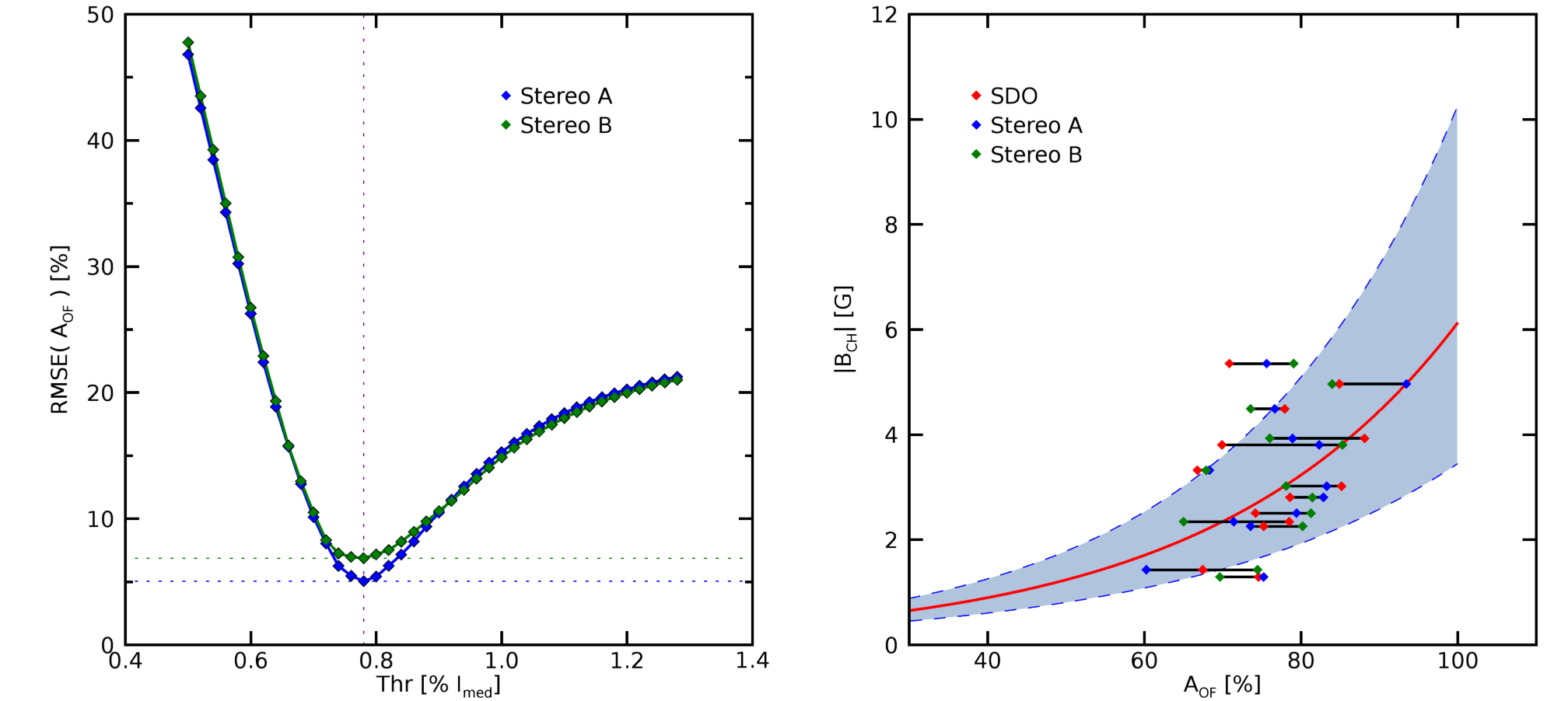
Figure 5.: Left: The RMSE between the percentage area coverage of STEREO and SDO is plotted as function of the $304$Å threshold to determine the threshold values most closely correlated between SDO and STEREO. Green represents STEREO-B and blue shows STEREO-A. The purple dashed line the minimum at $0.78\times I_{\mathrm{\textsc{SD},med}}$ for both STEREO-A (blue dashed line) and -B (green dashed line). Right: Coronal hole mean magnetic flux density ($|B_{\mathrm{\textsc{ch}}}|$) as function of the percentage area coverage ($A_{\mathrm{\textsc{of}}}$) for the minimum threshold as marked in the left panel. The percentage area coverage is plotted for SDO (red), STEREO-A (blue) and STEREO-B (green), a single coronal hole is connected by the black lines. The shaded area and red line show the fit and uncertainties derived in Figure fig:corrplot, a) from the full coronal hole sample. fig:stereo˙eval

Acknowledgments

The SDO and STEREO image data are available by courtesy of NASA and the respective science teams. S.G.H. acknowledges the German Data Center for SDO (GDC-SDO) for providing SDO data. Inspired by the International Space Science Institute (ISSI, Bern) Team on “Magnetic open flux and solar wind structuring in interplanetary space” (2019-2020).

Disclosure of Potential Conflicts of Interest

The authors declare that they have no conflicts of interest.

References

- Alves, Echer, and Gonzalez (2006) Alves, M.V., Echer, E., Gonzalez, W.D.: 2006, Geoeffectiveness of corotating interaction regions as measured by Dst index. Journal of Geophysical Research (Space Physics) 111, A07S05. DOI. ADS.
- Arge et al. (2010) Arge, C.N., Henney, C.J., Koller, J., Compeau, C.R., Young, S., MacKenzie, D., Fay, A., Harvey, J.W.: 2010, Air Force Data Assimilative Photospheric Flux Transport (ADAPT) Model. In: Maksimovic, M., Issautier, K., Meyer-Vernet, N., Moncuquet, M., Pantellini, F. (eds.) Twelfth International Solar Wind Conference, American Institute of Physics Conference Series 1216, 343. DOI. ADS.
- Arge et al. (2013) Arge, C.N., Henney, C.J., Hernandez, I.G., Toussaint, W.A., Koller, J., Godinez, H.C.: 2013, Modeling the corona and solar wind using ADAPT maps that include far-side observations. In: Zank, G.P., Borovsky, J., Bruno, R., Cirtain, J., Cranmer, S., Elliott, H., Giacalone, J., Gonzalez, W., Li, G., Marsch, E., Moebius, E., Pogorelov, N., Spann, J., Verkhoglyadova, O. (eds.) Solar Wind 13, American Institute of Physics Conference Series 1539, 11. DOI. ADS.
- Aschwanden et al. (2008) Aschwanden, M.J., Wülser, J.-P., Nitta, N.V., Lemen, J.R.: 2008, First Three-Dimensional Reconstructions of Coronal Loops with the STEREO A and B Spacecraft. I. Geometry. ApJ 679, 827. DOI. ADS.
- Berger and Title (2001) Berger, T.E., Title, A.M.: 2001, On the Relation of G-Band Bright Points to the Photospheric Magnetic Field. ApJ 553, 449. DOI. ADS.
- Boerner et al. (2014) Boerner, P.F., Testa, P., Warren, H., Weber, M.A., Schrijver, C.J.: 2014, Photometric and Thermal Cross-calibration of Solar EUV Instruments. Sol. Phys. 289, 2377. DOI. ADS.
- Bohlin and Sheeley (1978) Bohlin, J.D., Sheeley, N.R. Jr.: 1978, Extreme ultraviolet observations of coronal holes. II - Association of holes with solar magnetic fields and a model for their formation during the solar cycle. Sol. Phys. 56, 125. DOI. ADS.
- Couvidat et al. (2016) Couvidat, S., Schou, J., Hoeksema, J.T., Bogart, R.S., Bush, R.I., Duvall, T.L., Liu, Y., Norton, A.A., Scherrer, P.H.: 2016, Observables Processing for the Helioseismic and Magnetic Imager Instrument on the Solar Dynamics Observatory. Sol. Phys. 291, 1887. DOI. ADS.
- Cranmer (2009) Cranmer, S.R.: 2009, Coronal Holes. Living Reviews in Solar Physics 6, 3. DOI. ADS.
- Cranmer and van Ballegooijen (2005) Cranmer, S.R., van Ballegooijen, A.A.: 2005, On the Generation, Propagation, and Reflection of Alfvén Waves from the Solar Photosphere to the Distant Heliosphere. ApJS 156, 265. DOI. ADS.
- Dunn and Zirker (1973) Dunn, R.B., Zirker, J.B.: 1973, The Solar Filigree. Sol. Phys. 33, 281. DOI. ADS.
- Efron (1979) Efron, B.: 1979, Bootstrap methods: Another look at the jackknife. Ann. Statist. 7, 1. DOI. https://doi.org/10.1214/aos/1176344552.
- Efron and Tibshirani (1993) Efron, B., Tibshirani, R.J.: 1993, An Introduction to the Bootstrap, Chapman & Hall, New York.
- Farrugia, Burlaga, and Lepping (1997) Farrugia, C.J., Burlaga, L.F., Lepping, R.P.: 1997, Magnetic clouds and the quiet-storm effect at Earth. Washington DC American Geophysical Union Geophysical Monograph Series 98, 91. DOI. ADS.
- Feng et al. (2007) Feng, L., Inhester, B., Solanki, S.K., Wiegelmann, T., Podlipnik, B., Howard, R.A., Wuelser, J.-P.: 2007, First Stereoscopic Coronal Loop Reconstructions from STEREO SECCHI Images. ApJ 671, L205. DOI. ADS.
- Hahn, Landi, and Savin (2011) Hahn, M., Landi, E., Savin, D.W.: 2011, Differential Emission Measure Analysis of a Polar Coronal Hole during the Solar Minimum in 2007. ApJ 736, 101. DOI. ADS.
- Harvey, Sheeley, and Harvey (1982) Harvey, K.L., Sheeley, N.R. Jr., Harvey, J.W.: 1982, Magnetic measurements of coronal holes during 1975-1980. Sol. Phys. 79, 149. DOI. ADS.
- Hassler et al. (2020) Hassler, D.M., Newmark, J., Gibson, S., Harra, L., Appourchaux, T., Auchere, F., Berghmans, D., Colaninno, R., Fineschi, S., Gizon, L., Gosain, S., Hoeksema, T., Kintziger, C., Linker, J., Rochus, P., Schou, J., Viall, N., West, M., Woods, T., Wuelser, J.-P.: 2020, The Solaris Solar Polar Mission. In: EGU General Assembly Conference Abstracts, EGU General Assembly Conference Abstracts, 17703. ADS.
- Heinemann et al. (2018) Heinemann, S.G., Hofmeister, S.J., Veronig, A.M., Temmer, M.: 2018, Three-phase Evolution of a Coronal Hole. II. The Magnetic Field. ApJ 863, 29. DOI. ADS.
- Heinemann et al. (2019) Heinemann, S.G., Temmer, M., Heinemann, N., Dissauer, K., Samara, E., Jerčić, V., Hofmeister, S.J., Veronig, A.M.: 2019, Statistical Analysis and Catalog of Non-polar Coronal Holes Covering the SDO-Era Using CATCH. Sol. Phys. 294, 144. DOI. ADS.
- Heinemann et al. (2020) Heinemann, S.G., V., J., Temmer, M., Hofmeister, S.J., Dumbovi´c, M., Vennerstrom, S., Verbanac, G., Veronig, A.M.: 2020, A statistical study of the long-term evolution of coronal hole properties as observed by sdo. A&A 638, A68. DOI. https://doi.org/10.1051/0004-6361/202037613.
- Heinemann et al. (2021) Heinemann, S.G., Saqri, J., Veronig, A.M., Hofmeister, S.J., Temmer, M.: 2021, Statistical Approach on Differential Emission Measure of Coronal Holes using the CATCH Catalog. Sol. Phys. 296, 18. DOI. ADS.
- Hickmann et al. (2015) Hickmann, K.S., Godinez, H.C., Henney, C.J., Arge, C.N.: 2015, Data Assimilation in the ADAPT Photospheric Flux Transport Model. Sol. Phys. 290, 1105. DOI. ADS.
- Hofmeister et al. (2017) Hofmeister, S.J., Veronig, A., Reiss, M.A., Temmer, M., Vennerstrom, S., Vršnak, B., Heber, B.: 2017, Characteristics of Low-latitude Coronal Holes near the Maximum of Solar Cycle 24. ApJ 835, 268. DOI. ADS.
- Hofmeister et al. (2019) Hofmeister, S.J., Utz, D., Heinemann, S.G., Veronig, A., Temmer, M.: 2019, Photospheric magnetic structure of coronal holes. A&A 629, A22. DOI. ADS.
- Howard et al. (2008) Howard, R.A., Moses, J.D., Vourlidas, A., Newmark, J.S., Socker, D.G., Plunkett, S.P., Korendyke, C.M., Cook, J.W., Hurley, A., Davila, J.M., Thompson, W.T., St Cyr, O.C., Mentzell, E., Mehalick, K., Lemen, J.R., Wuelser, J.P., Duncan, D.W., Tarbell, T.D., Wolfson, C.J., Moore, A., Harrison, R.A., Waltham, N.R., Lang, J., Davis, C.J., Eyles, C.J., Mapson-Menard, H., Simnett, G.M., Halain, J.P., Defise, J.M., Mazy, E., Rochus, P., Mercier, R., Ravet, M.F., Delmotte, F., Auchere, F., Delaboudiniere, J.P., Bothmer, V., Deutsch, W., Wang, D., Rich, N., Cooper, S., Stephens, V., Maahs, G., Baugh, R., McMullin, D., Carter, T.: 2008, Sun Earth Connection Coronal and Heliospheric Investigation (SECCHI). Space Sci. Rev. 136, 67. DOI. ADS.
- Jin, Harvey, and Pietarila (2013) Jin, C.L., Harvey, J.W., Pietarila, A.: 2013, Synoptic Mapping of Chromospheric Magnetic Flux. ApJ 765, 79. DOI. ADS.
- Kaiser et al. (2008) Kaiser, M.L., Kucera, T.A., Davila, J.M., St. Cyr, O.C., Guhathakurta, M., Christian, E.: 2008, The STEREO Mission: An Introduction. Space Sci. Rev. 136, 5. DOI. ADS.
- Lemen et al. (2012) Lemen, J.R., Title, A.M., Akin, D.J., Boerner, P.F., Chou, C., Drake, J.F., Duncan, D.W., Edwards, C.G., Friedlaender, F.M., Heyman, G.F., Hurlburt, N.E., Katz, N.L., Kushner, G.D., Levay, M., Lindgren, R.W., Mathur, D.P., McFeaters, E.L., Mitchell, S., Rehse, R.A., Schrijver, C.J., Springer, L.A., Stern, R.A., Tarbell, T.D., Wuelser, J.-P., Wolfson, C.J., Yanari, C., Bookbinder, J.A., Cheimets, P.N., Caldwell, D., Deluca, E.E., Gates, R., Golub, L., Park, S., Podgorski, W.A., Bush, R.I., Scherrer, P.H., Gummin, M.A., Smith, P., Auker, G., Jerram, P., Pool, P., Soufli, R., Windt, D.L., Beardsley, S., Clapp, M., Lang, J., Waltham, N.: 2012, The Atmospheric Imaging Assembly (AIA) on the Solar Dynamics Observatory (SDO). Sol. Phys. 275, 17. DOI. ADS.
- Levine (1982) Levine, R.H.: 1982, Open magnetic fields and the solar cycle. I - Photospheric sources of open magnetic flux. Sol. Phys. 79, 203. DOI. ADS.
- Li, Feng, and Wei (2021) Li, H., Feng, X., Wei, F.: 2021, Comparison of Synoptic Maps and PFSS Solutions for The Declining Phase of Solar Cycle 24. Journal of Geophysical Research (Space Physics) 126, e28870. DOI. ADS.
- Liewer et al. (2014) Liewer, P.C., González Hernández, I., Hall, J.R., Lindsey, C., Lin, X.: 2014, Testing the Reliability of Predictions of Far-Side Active Regions from Helioseismology Using STEREO Far-Side Observations of Solar Activity. Sol. Phys. 289, 3617. DOI. ADS.
- Linker et al. (2017) Linker, J.A., Caplan, R.M., Downs, C., Riley, P., Mikic, Z., Lionello, R., Henney, C.J., Arge, C.N., Liu, Y., Derosa, M.L., Yeates, A., Owens, M.J.: 2017, The open flux problem. The Astrophysical Journal 848, 70. DOI. https://doi.org/10.3847%2F1538-4357%2Faa8a70.
- Linker et al. (2021) Linker, J.A., Heinemann, S.G., Temmer, M., Owens, M.J., Caplan, R.M., Arge, C.N., Asvestari, E., Delouille, V., Downs, C., Hofmeister, S.J., Jebaraj, I.C., Madjarska, M., Pinto, R., Pomoell, J., Samara, E., Scolini, C., Vrsnak, B.: 2021, Coronal Hole Detection and Open Magnetic Flux. arXiv e-prints, arXiv:2103.05837. ADS.
- Lowder, Qiu, and Leamon (2017) Lowder, C., Qiu, J., Leamon, R.: 2017, Coronal Holes and Open Magnetic Flux over Cycles 23 and 24. Sol. Phys. 292, 18. DOI. ADS.
- Müller et al. (2020) Müller, D., St. Cyr, O.C., Zouganelis, I., Gilbert, H.R., Marsden, R., Nieves-Chinchilla, T., Antonucci, E., Auchère, F., Berghmans, D., Horbury, T.S., Howard, R.A., Krucker, S., Maksimovic, M., Owen, C.J., Rochus, P., Rodriguez-Pacheco, J., Romoli, M., Solanki, S.K., Bruno, R., Carlsson, M., Fludra, A., Harra, L., Hassler, D.M., Livi, S., Louarn, P., Peter, H., Schühle, U., Teriaca, L., del Toro Iniesta, J.C., Wimmer-Schweingruber, R.F., Marsch, E., Velli, M., De Groof, A., Walsh, A., Williams, D.: 2020, The Solar Orbiter mission. Science overview. A&A 642, A1. DOI. ADS.
- Obridko and Shelting (1989) Obridko, V.N., Shelting, B.D.: 1989, Coronal holes as indicators of large-scale magnetic fields in the corona. Sol. Phys. 124, 73. DOI. ADS.
- Pesnell, Thompson, and Chamberlin (2012) Pesnell, W.D., Thompson, B.J., Chamberlin, P.C.: 2012, The Solar Dynamics Observatory (SDO). Sol. Phys. 275, 3. DOI. ADS.
- Petrie (2015) Petrie, G.J.D.: 2015, Solar Magnetism in the Polar Regions. Living Reviews in Solar Physics 12, 5. DOI. ADS.
- Petrie and Haislmaier (2013) Petrie, G.J.D., Haislmaier, K.J.: 2013, Low-latitude Coronal Holes, Decaying Active Regions, and Global Coronal Magnetic Structure. ApJ 775, 100. DOI. ADS.
- Pomoell and Poedts (2018) Pomoell, J., Poedts, S.: 2018, EUHFORIA: European heliospheric forecasting information asset. Journal of Space Weather and Space Climate 8, A35. DOI. ADS.
- Richardson (2018) Richardson, I.G.: 2018, Solar wind stream interaction regions throughout the heliosphere. Living Reviews in Solar Physics 15, 1. DOI. ADS.
- Saqri et al. (2020) Saqri, J., Veronig, A.M., Heinemann, S.G., Hofmeister, S.J., Temmer, M., Dissauer, K., Su, Y.: 2020, Differential Emission Measure Plasma Diagnostics of a Long-Lived Coronal Hole. Sol. Phys. 295, 6. DOI. ADS.
- Schou et al. (2012) Schou, J., Scherrer, P.H., Bush, R.I., Wachter, R., Couvidat, S., Rabello-Soares, M.C., Bogart, R.S., Hoeksema, J.T., Liu, Y., Duvall, T.L., Akin, D.J., Allard, B.A., Miles, J.W., Rairden, R., Shine, R.A., Tarbell, T.D., Title, A.M., Wolfson, C.J., Elmore, D.F., Norton, A.A., Tomczyk, S.: 2012, Design and Ground Calibration of the Helioseismic and Magnetic Imager (HMI) Instrument on the Solar Dynamics Observatory (SDO). Sol. Phys. 275, 229. DOI. ADS.
- Solanki et al. (2020) Solanki, S.K., del Toro Iniesta, J.C., Woch, J., Gandorfer, A., Hirzberger, J., Alvarez-Herrero, A., Appourchaux, T., Martínez Pillet, V., Pérez-Grande, I., Sanchis Kilders, E., Schmidt, W., Gómez Cama, J.M., Michalik, H., Deutsch, W., Fernandez-Rico, G., Grauf, B., Gizon, L., Heerlein, K., Kolleck, M., Lagg, A., Meller, R., Müller, R., Schühle, U., Staub, J., Albert, K., Alvarez Copano, M., Beckmann, U., Bischoff, J., Busse, D., Enge, R., Frahm, S., Germerott, D., Guerrero, L., Löptien, B., Meierdierks, T., Oberdorfer, D., Papagiannaki, I., Ramanath, S., Schou, J., Werner, S., Yang, D., Zerr, A., Bergmann, M., Bochmann, J., Heinrichs, J., Meyer, S., Monecke, M., Müller, M.-F., Sperling, M., Álvarez García, D., Aparicio, B., Balaguer Jiménez, M., Bellot Rubio, L.R., Cobos Carracosa, J.P., Girela, F., Hernández Expósito, D., Herranz, M., Labrousse, P., López Jiménez, A., Orozco Suárez, D., Ramos, J.L., Barandiarán, J., Bastide, L., Campuzano, C., Cebollero, M., Dávila, B., Fernández-Medina, A., García Parejo, P., Garranzo-García, D., Laguna, H., Martín, J.A., Navarro, R., Núñez Peral, A., Royo, M., Sánchez, A., Silva-López, M., Vera, I., Villanueva, J., Fourmond, J.-J., de Galarreta, C.R., Bouzit, M., Hervier, V., Le Clec’h, J.C., Szwec, N., Chaigneau, M., Buttice, V., Dominguez-Tagle, C., Philippon, A., Boumier, P., Le Cocguen, R., Baranjuk, G., Bell, A., Berkefeld, T., Baumgartner, J., Heidecke, F., Maue, T., Nakai, E., Scheiffelen, T., Sigwarth, M., Soltau, D., Volkmer, R., Blanco Rodríguez, J., Domingo, V., Ferreres Sabater, A., Gasent Blesa, J.L., Rodríguez Martínez, P., Osorno Caudel, D., Bosch, J., Casas, A., Carmona, M., Herms, A., Roma, D., Alonso, G., Gómez-Sanjuan, A., Piqueras, J., Torralbo, I., Fiethe, B., Guan, Y., Lange, T., Michel, H., Bonet, J.A., Fahmy, S., Müller, D., Zouganelis, I.: 2020, The Polarimetric and Helioseismic Imager on Solar Orbiter. A&A 642, A11. DOI. ADS.
- Temmer, Hinterreiter, and Reiss (2018) Temmer, M., Hinterreiter, J., Reiss, M.A.: 2018, Coronal hole evolution from multi-viewpoint data as input for a stereo solar wind speed persistence model. J. Space Weather Space Clim. 8, A18. DOI. https://doi.org/10.1051/swsc/2018007.
- Verbeeck et al. (2014) Verbeeck, C., Delouille, V., Mampaey, B., De Visscher, R.: 2014, The SPoCA-suite: Software for extraction, characterization, and tracking of active regions and coronal holes on EUV images. A&A 561, A29. DOI. ADS.
- Vršnak et al. (2017) Vršnak, B., Dumbović, M., Čalogović, J., Verbanac, G., Poljančić Beljan, I.: 2017, Geomagnetic Effects of Corotating Interaction Regions. Sol. Phys. 292, 140. DOI. ADS.
- Wallace et al. (2019) Wallace, S., Arge, C.N., Pattichis, M., Hock-Mysliwiec, R.A., Henney, C.J.: 2019, Estimating Total Open Heliospheric Magnetic Flux. Sol. Phys. 294, 19. DOI. ADS.
- Wang, Hawley, and Sheeley (1996) Wang, Y.-M., Hawley, S.H., Sheeley, N.R. Jr.: 1996, The Magnetic Nature of Coronal Holes. Science 271, 464. DOI. ADS.
- Warren and Hassler (1999) Warren, H.P., Hassler, D.M.: 1999, The density structure of a solar polar coronal hole. J. Geophys. Res. 104, 9781. DOI. ADS.
- Wedemeyer-Böhm, Lagg, and Nordlund (2009) Wedemeyer-Böhm, S., Lagg, A., Nordlund, Å.: 2009, Coupling from the Photosphere to the Chromosphere and the Corona. Space Sci. Rev. 144, 317. DOI. ADS.
- Wendeln and Landi (2018) Wendeln, C., Landi, E.: 2018, EUV Emission and Scattered Light Diagnostics of Equatorial Coronal Holes as Seen by Hinode/EIS. ApJ 856, 28. DOI. ADS.
- Wiegelmann and Solanki (2004) Wiegelmann, T., Solanki, S.K.: 2004, Similarities and Differences between Coronal Holes and the Quiet Sun: Are Loop Statistics the Key? Sol. Phys. 225, 227. DOI. ADS.
- Wilcox (1968) Wilcox, J.M.: 1968, The Interplanetary Magnetic Field. Solar Origin and Terrestrial Effects. Space Sci. Rev. 8, 258. DOI. ADS.