Analytical perturbation theory and Nucleon structure function in infrared region

Abstract

We employ analytic QCD (anQCD) approach to analyze the unpolarized nucleon structure function (NSF) in deep inelastic scattering ( DIS ) processes at the next-to-leading order (NLO) accuracy. Considering the unreliable results of underlying perturbative QCD (pQCD) at energy scale $Q^{2}\sim\Lambda^{2}$ and even less we modify the calculations at these scales using anQCD approach and compare them with results from underlying pQCD and also with the available experimental data. In these progresses the massive perturbation theory (MPT) model is also used where an effective mass is attributed to gluons. We finally use the Jacobi polynomials formalism to transfer the calculations from Mellin moment space to Bjorken-$x$ space. To confirm the validity of anQCD approach the Gottfired sum rule is also investigated. The achieved numerical results at low energy scales are compatible with what is expected and corresponding to an admissible behaviour of parton densities.

I Introduction

An observable should be an analytic (holomorphic) function in the complex $Q^{2}$ plane where $Q^{2}\not<0$. At high energy scales, i.e. $|Q^{2}|\gg 1$, we can have a good theoretical description and achieve reliable results which are confirming experimental data, using underlying pQCD. But at the energy scale near to QCD cutoff parameter, i.e., $Q^{2}\sim\Lambda^{2}$ and less, the coupling constant of QCD starts to be growing rapidly and as a result, facing Landau IR-singularities. On the other hand the spacelike QCD observable, such as the nucleon structure functions, do not have such singularities. Accordingly one cannot obtain any reliable results from underlying pQCD, thence we need an efficient approach which eliminates these singularities in order to achieve suitable results. There are various approaches to attain this goal such as Brodsky coupling constant achievement by Ads/CFT Brodsky:2010ur , the dispersive approach of Dokshitzer Dokshitzer:1995qm ; Dokshitzer:1995zt and finally Analytic Perturbation Theory(APT)ShS ; MS ; MSS ; MSa ; Sh1 ; Sh2 . We use the last one to shift and even eliminates the mentioned singularities in calculations of physical quantities such as unpolarized nucleon structure function (NSF) and also the Gottfried sum rule, and thus modify their theoretical predictions. We refer to Ours for recent related work. In this approach, the running QCD coupling constant ($a(Q^{2})=\frac{\alpha_{s}(Q^{2})}{\pi}$) is transformed in an analytic function of $Q^{2}$ (analytic for $Q^{2}\not<0$) which is called analytic QCD coupling constant [$A_{1}(Q^{2})$] that does not have any Landau singularities and we are able to calculate the results for the quantities without any such singularities at the low energies, using the analytic coupling constant.

Among the approaches which eliminate the Landau singularities, we can refer to Fractional Analytic Perturbation Theory [FAPT] BMS1 ; BMS2 ; BMS3 ; Ayala:2014pha ; $2\delta$anQCD 2danQCD ; Ayala:2014pha and $3\delta$anQCD 3danQCD which are based on parameterising the spectral function at low energies by two or three Dirac delta functions, respectively; and finally massive perturbation theory (MPT) MPT ; Ayala:2014pha which is based on removing the Landau singularities by shifting them into the timelike region. As an attribute that the last method possesses, it considers an effective mass for the gluon. Since we are working on nucleon structure function which contains the singlet and gluon sectors , we decide to apply it so that we can achieve better computational results.

The organization of this paper is as follows. In next section a brief description of essential concepts of APT is reviewed. In Sec.III evolution of parton densities and nucleon structure function, using Jacobi transformation are discussed. Sec.IV is devoted to illustration of the structure function in MPT model. Based on this model the Gottfired sum rule is considered in Sec.V. Finally summary and conclusion is presented in Sec.VI

II Basic concepts in analytic perturbation theory

As we mentioned, underlying pQCD coupling suffers from unphysical Landau singularities at $Q^{2}\sim\Lambda^{2}$ . Therefore we can not apply it in the low momentum and that is a motivation to use other approaches, especially analytic QCD (anQCD) to achieve fairly accurate results for physical quantities. In this approach we have analytic couplings $A_{\nu}$ which are free from aforementioned problems. In the following content we will represent the main elements of APT. Application of Cauchy theorem to the running coupling $a(Q^{2})$, where $a(Q^{2})=\alpha_{s}(Q^{2})/\pi$, gives us the following spectral relation in general anQCD Ayala:2014pha ; Ayala_2015 :

$$A_{1}(Q^{2})=\frac{1}{\pi}\int_{\sigma=M_{th}^{2}}^{\infty}\frac{d\sigma\rho_{1}(\sigma)}{(\sigma+Q^{2})}\;,$$ (1)

where

$${{}\rho_{1}(\sigma)\equiv ImA_{1}(-\sigma-i\varepsilon)\;.}$$ (2)

Different approaches to consider the discontinuity function $\rho_{1}({\sigma})$ and the coupling function $A_{1}(Q^{2})$ will lead to the various anQCD models. As we pointed out before $A_{1}(Q^{2})$ is the anQCD-analog of the underlying pQCD coupling $a(Q^{2})=\alpha_{s}(Q^{2})/\pi$, i.e., at $\sigma\gg\Lambda$ we have ${\equiv Im}a(-\sigma-i\varepsilon)={\equiv Im}A_{1}(-\sigma-i\varepsilon)$. Let us denote by $A_{\nu}$ the anQCD-analog of the pQCD power $a^{\nu}$ (where $\nu$ is not necessarily integer). As an important point we should notice that there is not standard algebra for $A_{\nu}$, i.e., $A_{\nu}A_{\mu}\not\equiv A_{\nu+\mu}$ or $A_{\nu+\mu}\not\equiv(A_{\nu})^{\mu}$. For the construction of $A_{\nu}$ in a general anQCD, we follow Ref. Cveti__2012 .

Correct analogs $A_{n}(Q^{2})$ of the powers $a^{n}(Q^{2})$ will be achieved, using the logarithmic derivatives of $A_{1}$ Ayala:2014pha :

$${{\widetilde{\mathcal{A}}}}_{n+1}\equiv\frac{(-1)^{n}}{\beta_{0}^{n}n!}(\frac{\partial}{\partial lnQ^{2}})^{n}A_{1}(Q^{2})\;.$$ (3)

It is obvious that with n=0 we get ${\widetilde{\mathcal{A}}}_{1}\equiv A_{1}$. Here $\beta_{0}=\frac{1}{4}(11-\frac{2}{3}N_{f})$ is the first coefficient of QCD-$\beta$ function which is scheme independent where this function is governing by Renormalization Group Equation (RGE) for QCD runnning coupling constant. Substituting $A_{1}$ in Eq.(1) into Eq.(3) will lead to

$${\widetilde{\mathcal{A}}}_{n+1}(Q^{2})=\frac{1}{\pi}\frac{(-1)}{\beta_{0}^{n}\Gamma(n+1)}\int_{0}^{\infty}\frac{d\sigma}{\sigma}\rho_{1}(\sigma)Li_{-n}(\frac{-\sigma}{Q^{2}})\;.$$ (4)

In this equation $n$ is an integer number and it can be extended to noninteger index $\nu$ as follows Cveti__2012 :

$${\widetilde{\mathcal{A}}}_{\nu+1}(Q^{2})=\frac{1}{\pi}\frac{(-1)}{\beta_{0}^{\nu}\Gamma(\nu+1)}\int_{0}^{\infty}\frac{d\sigma}{\sigma}\rho_{1}(\sigma)Li_{-\nu}(\frac{-\sigma}{Q^{2}})\;.$$ (5)

Here $Li_{-\nu}(\frac{-\sigma}{Q^{2}})$ is polylogarithm function. It should be noted that the integral in Eq.(5) is converging at low $\sigma$ for $\nu>-1$ where polyloghartitm function is approximated by $Li_{-\nu}(-z)\sim ln^{-\nu}z$. The analytic analogs $A_{\nu}(Q^{2})$ can be constructed as linear combinations of ${\widetilde{\mathcal{A}}}_{\nu+m}$’s:

$$A_{\nu}(Q^{2})={{\widetilde{\mathcal{A}}}}_{\nu}+\sum_{{m\geq 1}}{{\widetilde{k}}}_{m}(\nu){{\widetilde{\mathcal{A}}}}_{\nu+m}\;.$$ (6)

The coefficients ${{\widetilde{k}}}_{m}(\nu)$ in Eq.(6) have been determined in Cveti__2012 . Using the analytic coupling constant we can do the required calculations for quantities which contain noninteger power expansion of the coupling constant.

The specific anQCD model that has been used in this paper, is named Massive Perturbation Theory (MPT) in which to achieve a holomorphic coupling, an effective mass is attributed to gluon such as MPT ; Ayala:2014pha

$$A_{1}^{(MPT)}(Q^{2},N_{f})=a(Q^{2}+m_{gl}^{2},N_{f})\;.$$ (7)

The mass scale $m_{gl}\sim 0.5-1\;GeV$ refers to gluon mass where $m_{gl}^{2}=0.7Gev^{2}$ is considered here. Since $m_{gl}^{2}>\Lambda^{2}$, we get a coupling that is analytic even to scales less than $\Lambda$. At high energy $A_{1}^{MPT}(Q^{2})$ tends to the pQCD coupling $a(Q^{2})$ . It can be seen that the difference of MPT with respect to the underlying pQCD coupling would be given by Ayala:2014pha :

$$A_{1}^{MPT}(Q^{2},N_{f})-a(Q^{2},N_{f})\sim\frac{m_{gl}^{2}}{Q^{2}ln^{2}(\frac{Q^{2}}{\Lambda^{2}})}\;.$$ (8)

In the following sections we can observe the benefits of MPT model in comparing with pQCD approach. As an adjunct to this issue we plot in Fig.1 the running coupling constant in two MPT and FAPT models and compare it with the underlying pQCD coupling

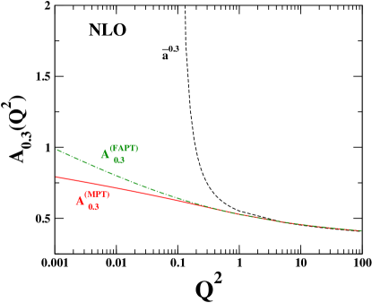
Figure 1: (Color online) The coupling constants, using two MPT and FAPT models with fraction index $\nu$ =0.3, are presenting. The moderate behaviour of the running coupling constant in these models at low energy scales in comparison to underlying pQCD is obvious.

III Jacobi transformation and parton densities evolutions

To extract the unpolarized NSF in terms of $Q^{2}$ energy scale we need to do the energy evolution for both the singlet and nonsinglet sectors of SF. Here we start by singlet densities where splitting functions are governing their evolution. The singlet quark distribution of hadron is defined by

$$\Sigma(x,Q^{2})=\sum_{i=1}^{N_{f}}[q_{i}(x,Q^{2})+\bar{q_{i}}(x,Q^{2})]\;.$$ (9)

Here $q_{i}(x,Q^{2})$ and $\bar{q_{i}}(x,Q^{2})$ represent the respective number densities of quarks and antiquarks as a function of the carried momentum fraction x. The subscript i indicates the flavor of the (anti)quark and $n_{f}$ stands for the the number of effectively massless flavours. Suppressing the fractional dependencies, the coupled evolution equations for the singlet patron and gluon distributions read

$$\frac{d}{dlnQ^{2}}\begin{pmatrix}\Sigma\\ g\end{pmatrix}=\begin{pmatrix}P_{qq}&P_{qg}\\ P_{gq}&P_{gg}\end{pmatrix}\otimes\begin{pmatrix}\Sigma_{0}\\ g_{0}\end{pmatrix},$$ (10)

where $\otimes$ stands for convolution integral in the momentum variable,

$$[a\otimes b](x)\equiv\int_{x}^{1}\frac{dy}{y}a(y)b(\frac{x}{y}).$$ (11)

The corresponding gluon distribution, $g(x,Q^{2})$, is denoted briefly here by $g$.

The quark-quark splitting function $P_{qq}\leavevmode\nobreak\$Floratos:1981hs in Eq.(10) can be expressed as Vogt:2004ns

$$P_{qq}=P_{ns}^{+}+N_{f}(P_{\bar{q}q}^{s}+P_{{q}q}^{s})\equiv P_{ns}^{+}+P_{ps}\;.$$ (12)

Here $P_{ns}^{+}$ is the non-singlet splitting function. The quantities $P_{qq}^{s}$ and $P_{\bar{q}q}^{s}$ are the flavour independent sea contributions to the quark-quark and quark-antiquark splitting functions respectively. The gluon-quark entries in Eq.(10) are given by

$$P_{qg}=N_{f}P_{q_{i}g},\;\;P_{gq}=P_{gq_{i}}\;.$$ (13)

In terms of the flavour independent splitting functions one can write $P_{q_{i}g}=P_{\bar{q}g}$ and $P_{gq_{i}}=P_{g\bar{q}}$.

The required calculations can now be continued in Mellin-N space, using Mellin transformation:

$$a(N)=\int_{0}^{1}dxx^{N-1}a(x)\;.$$ (14)

Then by transforming all needed quantities to Mellin (moment) space, the solution of Eq.(10) at NLO accuracy is rendered by:

$$\begin{pmatrix}\Sigma\\ g\end{pmatrix} = \Bigg{\{}\left(\frac{a_{s}}{a_{0}}\right)^{-r_{-}}\bigg{[}\,\mbox{\boldmath$e$}_{-}+(a_{0}-a_{s})\>\mbox{\boldmath$e$}_{-}\mbox{\boldmath$R$}_{1}\mbox{\boldmath$e$}_{-}$$ (15)

$$\qquad\mbox{}-\bigg{(}a_{0}-a_{s}\left(\frac{a_{s}}{a_{0}}\right)^{r_{-}-r_{+}}\bigg{)}\,\frac{\mbox{\boldmath$e$}_{-}\mbox{\boldmath$R$}_{1}\mbox{\boldmath$e$}_{+}}{r_{+}-r_{-}-1}\,\bigg{]}\>$$

$$+\>(\,+\leftrightarrow-\,)\Bigg{\}}\begin{pmatrix}\Sigma_{0}\\ g_{0}\end{pmatrix}\;.$$

Here we explicitly define $a_{s}=\alpha_{s}/(4\pi)=a/4$. In the last line the following recursive abbreviations have been used Vogt:2004ns

$$\mbox{\boldmath$R$}_{0}\> \equiv \>\frac{1}{\beta_{0}}\mbox{\boldmath$P$}^{(0)}\>\>,$$

$$\mbox{\boldmath$R$}_{k}\> \equiv \>\frac{1}{\beta_{0}}\mbox{\boldmath$P$}^{(k)}-\sum_{i=1}^{k}b_{i}\,\mbox{\boldmath$R$}_{k-i}\;,$$ (16)

with $b_{k}\equiv\beta_{k}/\beta_{0}$. Furthermore for the $r_{\pm}$ one can write

$$r_{\pm}=\frac{1}{2\beta_{0}}\left[P_{qq}^{0}+P_{gg}^{0}\pm\sqrt{(P_{qq}^{0}-P_{gg}^{0})^{2}-4P_{qg}^{0}P_{gq}^{0}}\right]\;,$$ (17)

where the following relation for $\mbox{\boldmath$e$}_{\pm}$ is defined:

$$\mbox{\boldmath$e$}_{\pm}=\frac{1}{r_{\pm}-r_{\mp}}\Big{[}\mbox{\boldmath$R$}_{0}-r_{\mp}\,\mbox{\boldmath$I$}\Big{]}\;,$$ (18)

in which  $I$ is representing a unique $2\times 2$ matrix.

In non-singlet case in order to decouple the combination, it is needed to use the general structure of (anti-) quark (anti-) quark splitting functions as it followsVogt:2004ns

$$P_{q_{i}q_{k}} =P_{\bar{q}_{i}\bar{q}_{k}}=\delta_{ik}P_{qq}^{V}+P_{qq}^{s}\;,$$ (19)

$$P_{q_{i}\bar{q}_{k}} =P_{\bar{q}_{i}q_{k}}=\delta_{ik}P_{q\bar{q}}^{V}+P_{q\bar{q}}^{s}$$

The flavour asymmetries $q_{ns}^{\pm}$ and the total valence distribution $q_{ns}^{V}$ and their corresponding splitting functions are given by Vogt:2004ns ,

$$q_{ns,ik}^{\pm} =q_{i}\pm\bar{q}_{i}-(q_{k}\pm\bar{q}_{k})\;,$$ (20)

$$q_{ns}^{V} =\sum_{r=1}^{n_{f}}(q_{r}-\bar{q}_{r})\;,$$

$$P_{ns}^{\pm} =P_{qq}^{V}\pm P_{q\bar{q}}^{V}\;,$$

$$P_{ns}^{V} =P_{qq}^{V}-P_{q\bar{q}}^{V}+n_{f}(P_{qq}^{s}-P_{q\bar{q}}^{s})\equiv P_{ns}^{-}+P_{ns}^{s}\;.$$

For non-singlet quark distributions evolution a similar process exists like the singlet case, but with the obvious simplification that no spurious complexity occur. Consequently the non-singlet evolution can be written as it follows Vogt:2004ns :

$$\begin{aligned} q^{\pm,V}(a_{s})={}&exp\Bigg{[}R_{1}^{\pm,V}(a_{0}-a_{s})\Bigg{]}\Bigg{(}\frac{a_{s}}{a_{0}}\Bigg{)}^{-R_{0}^{\pm,V}}\\ \times q^{\pm,V}(a_{0})\end{aligned}$$ (21)

In which $R_{0}^{\pm,V}=\frac{1}{\beta_{0}}P^{(0)\pm,V}$ and $R_{1}^{\pm,V}=\frac{1}{\beta_{0}}P^{(1)\pm,V}-\beta_{1}R_{0}^{\pm,V}$ are defined based on non-singlet splitting functions where $\beta_{0}$ and $\beta_{1}$ are the first two universal coefficient of QCD $\beta$-function . Accordingly Eq.(21) at next-to-leading-order (NLO) accuracy can be written:

$$\begin{aligned} q^{\pm,V}_{NLO}(a_{s})={}&\Bigg{[}1+R_{1}^{\pm,V}(a_{0}-a_{s})\Bigg{]}(\frac{a_{s}}{a_{0}})^{-R_{0}^{\pm,V}}\\ &\times q^{\pm,V}(a_{0})\;.\end{aligned}$$ (22)

Finally, using Eq.(15) and Eq.(22) we can obtain the nucleon structure function at the NLO accuracy in Mellin (moment) N-space as it follows

$$F_{2}(N,Q^{2}) = [C_{2q}^{(0)}(N)+a_{s}(Q^{2})C_{2q}^{(1)}(N)]\sum_{i=u,d,s}e_{i}^{2}q_{i}(N,Q^{2})$$ (23)

$$+a_{s}(Q^{2})C_{2g}^{(1)}(N)\frac{1}{f}\sum_{i=u,d,s}e_{i}^{2}g(N,Q^{2})\;.$$

Here $C^{k}(N)$s are Wilson coefficient functions which have been calculated in Vogt:2004mw . Using Jacobi transformation, as was mentioned before, is an adequate method to convert the calculated results from moment N-space to Bjorken x-space. Details of this method has been described in Koekoek_2000 . According to this method we can define the NSF, based on the following relation:

$$F_{2}(x,Q^{2})=x^{\beta}(1-x)^{\alpha}\sum_{x=0}^{\infty}a_{n}^{\alpha,\beta}(Q^{2})\Theta_{n}^{(\alpha,\beta)}(x)\;.$$ (24)

Here $a_{n}^{\alpha,\beta}(Q^{2})$ is an expansion coefficient and $\Theta_{n}^{(\alpha,\beta)}(x)$ is denoting to the Jacobi polynomials and they are related to each other by:

$$a_{n}^{\alpha,\beta}(Q^{2})=\int_{0}^{1}F_{2}(x,Q^{2})\Theta_{n}^{(\alpha,\beta)}(x)dx\;.$$ (25)

By sunstituting $\Theta_{n}^{(\alpha,\beta)}(x)=\sum_{k=0}^{n}C_{k,n}^{(\alpha,\beta)}x^{k}$ in Eq.( 25) one can get:

$$a_{n}^{\alpha,\beta}(Q^{2})=\int_{0}^{1}F_{2}(x,Q^{2})\sum_{j=0}^{n}C_{j,n}^{(\alpha,\beta)}x^{j}dx$$ (26)

Putting Eq.(26) into Eq.(24) and using the SF in moment-N space by$M_{F_{2}}(N,Q^{2})=\int_{0}^{1}x^{j-2}F_{2}(x,Q^{2})dx$ we can achive to SF in Bjorken x-pace as it follows Kataev:1997nc :

$$F_{2}(x,Q^{2})=x^{\beta}(1-x)^{\alpha}\sum_{n=0}^{N_{max}}\Theta_{n}^{(\alpha,\beta)}(x)$$

$$\sum_{j=0}^{n}C_{j,n}^{(\alpha,\beta)}M_{F_{2}}(j+2,Q^{2})$$ (27)

IV Unpolarized nucleon structure function and the MPT model

To do the required computations to extract the nucleon structure function we need first the parton distribution functions (PDFs) at initial energy scale, $Q_{0}$, as the inputs. For this purpose the following parameterized functions are suggested Jimenez_Delgado_2014 .

$$\begin{gathered}xu_{v}(x,Q_{0}^{2})=N_{u}x^{a_{u}}(1-x)^{b_{u}}(1+A_{u}\sqrt{x}+B_{u}x+C_{u}x^{2}),\\ xd_{v}(x,Q_{0}^{2})=N_{d}x^{a_{d}}(1-x)^{b_{d}}(1+A_{d}\sqrt{x}+B_{d}x+C_{d}x^{2}),\\ xg(x,Q_{0}^{2})=N_{g}x^{a_{g}}(1-x)^{b_{g}}(1+B_{g}x^{\alpha_{g}}(1-x)^{\beta_{g}}),\\ x\Sigma(x,Q_{0}^{2})=N_{\Sigma}x^{a_{\Sigma}}(1-x)^{b_{\Sigma}}(1+A_{\Sigma}\sqrt{x}+B_{\Sigma}x),\\ x\Delta(x,Q_{0}^{2})=N_{\Delta}x^{a_{\Delta}}(1-x)^{b_{\Delta}}(1+A_{\Delta}\sqrt{x}+B_{\Delta}x),\\ xs(x,Q_{0}^{2})=N_{s}x^{a_{s}}(1-x)^{b_{s}}(1+A_{s}\sqrt{x}+B_{s}x)\end{gathered}$$ (28)

In Eq.(28) these definitions are used: $u_{v}=u-\bar{u}$, $d_{v}=d-\bar{d}$, $\Sigma=\bar{u}+\bar{d}$ and $\Delta=\bar{d}-\bar{u}$. All unknown parameters, including the normalization factors are obtained via the fitting over the related data Jimenez_Delgado_2014 . The results are listed in Table.2.

NLO
Nu	1.63	Nd	7.4	Ng	2.95
au	0.55	ad	0.92	ag	0.047
bu	3.61	bd	4.6	bg	6.1
Au	0.8	Ad	-2.8	Bg	0
Bu	4.7	Bd	4.5	$\alpha_{g}$	0
Cu	-0.1	Cd	-2	$\beta_{g}$	0
NΣ	0.164	NΔ	57	Ns	0.03
aΣ	-0.19	aΔ	2.29	as	-0.28
bΣ	8.42	bΔ	18.6	bs	8.42
AΣ	1.9	AΔ	1	As	1.9
BΣ	10	BΔ	0	Bs	10

Table 1: Numerical values of the free parameters in Eq. (28) at $Q_{0}^{2}=2\;GeV^{2}$ in the NLO accuracy  Jimenez_Delgado_2014 .

The computations of this paper is done in mathematica environment, using anQCD.m package Ayala:2014pha and we are going to calculate analytic coupling constant corresponding to the underlying pQCD coupling, realising the presented powers in Eq.(23). The relevant mathematica command of MPT coupling constant is $AMPTNl[N_{f},\nu,Q^{2},m_{gl}^{2},\Lambda^{2}]$ which returns the N-loop ($N=1,2,3,4$) analytic MPT coupling $A_{\nu}^{(MPT,N)}(Q^{2},m_{gl}^{2},N_{f})$, including the fractional index $\nu$ at fixed number of active quark flavours $N_{f}$, with $Q^{2}$ in the Euclidean domain ($Q^{2}>0$). In as much we do calculations at NLO approximation, the $N$-loop is fixed at 2 (i.e., we use 2-loop MPT). The other commands of various anQCD models, for analytic coupling constant achievement, have been described in Ayala:2014pha . Interested reader is encouraged to read also Cveti__2012 . For simplicity we use the the notation $a_{s}^{\nu}\equiv\frac{a^{\nu}}{4^{\nu}}$ and subsequently $A_{s,\nu}\equiv\frac{A_{\nu}}{4^{\nu}}$, so the mentioned command becomes $\frac{AMPT2l[3,\nu,Q^{2},m_{gl}^{2},\Lambda^{2}]}{4^{\nu}}$. Here $N_{f}=3$, $m_{gl}^{2}=0.7$ $GeV^{2}$ and $\Lambda^{2}=0.35\;GeV^{2}$.

To employ the MPT model to extract the nucleon structure function, one may do it by applying the model to the evolution equations for singlet and non-singlet sectors of parton densities, given by Eq.(15) and Eq.(22) and finally using the MPT model separately to Eq.(23), containing the Wilson coefficients. This is not admissible since Wilson coefficients and parton densities are not directly observable and it is the nucleon structure function that should be analyzed, and not the factors separately. On this based we need to resort to Eq.(23) and employ the MPT model entirely on it. Hence each analytical coupling constant is utilized where part of its total exponent number is coming from the evolved parton densities and the rest is back to exponent of coupling constant behind Wilson factors. This procedure is completely corresponding to the property of analytical couplings, presented before by $A_{\nu}A_{\mu}\neq A_{\nu+\mu}$ or $A_{\nu+\mu}\neq(A_{\nu})^{\mu}$.

In fact what we need lastly to calculate can be given summarily by:

$$F_{2}(N,A_{\nu+1}(Q^{2}))=[C_{2q}^{(0)}(N)+A_{1}(Q^{2})C_{2q}^{(1)}(N)]$$

$$\sum_{i=u,d,s}e_{i}^{2}q_{i}(N,A_{\nu}(Q^{2}))+A_{1}(Q^{2})C_{2g}^{(1)}(N)\times$$

$$\frac{1}{f}\sum_{i=u,d,s}e_{i}^{2}g(N,A_{\nu}(Q^{2}))\;,$$ (29)

where we replace $A_{1}A_{\nu}\mapsto A_{\nu+1}$ ($\not=A_{1}A_{\nu}$).

Considering the numerical values for the required paremeters in analytical coupling, the utilized Mathematica command for $A_{\nu}(Q^{2})$ coupling would be $AMPT2l[3,\nu,Q^{2},0.7,0.35]$ where $\nu$ index is determined via the evolution processes for singlet and gluon densities and also non-singlet density. In practical calculations this index takes the following qualities: $\nu=-R_{0},1-R_{0},2-R_{0},-r_{-},1-r_{-},2-r_{-},r_{+},1-r_{+},2-r_{+}$.

Using available data at different energy scales, makes us the possibility to present the $Q$ dependence of $\alpha$ and $\beta$ Jocobbi parameters in Eq.(III) as are following:

$$\alpha = -465.737+553.088\;\exp(Q^{2})+\frac{336.376}{\log(Q^{2})}$$

$$\beta = 11.158+\frac{7.670Q^{2}}{\log(Q^{2})}+14.308\;\sqrt{Q^{2}}\;\log(Q^{2})$$

We depict in Fig.2 the $F_{2}^{p}(x,Q^{2})$ structure function verses $x$ Bjorken variable at different energy scales $Q^{2}=0.15,0.21,0.27$ and $0.313$ $GeV^{2}$, using MPT modle and compare them with E665 experimental data E665:1996mob . To indicate the adequate applicability of MPT model at low energy scales we also add to this figure the results of underlying pQCD for the $F_{2}^{p}(x,Q^{2})$ structure function. To achieve more precise results, the computation of underlying pQCD are done at the two loops approximation of coupling constant  Cafarella:2005zj ; vanNeerven:1999ca ; vanNeerven:2000uj ; JimenezDelgado:2008rdu .

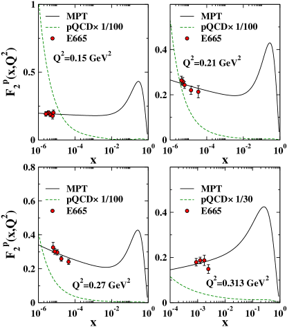
Figure 2: (Color online) Unpolarized nucleon structure function, $F_{2}^{p}(x,Q^{2})$, as a function of $x$-Bjorken variable, using MPT model (solid line) and underlying pQCD (dashed line). Comparison with the available experimental data E665:1996mob

has also been done.

There is a few experimental data in mentioned energies but as it is shown in Fig.2, an appropriate agreement is standing between anQCD results and the available experimental data.

V Gottfried sum rule in anQCD approach

Since the advent of quark-parton model, sum rules for nucleon structure functions play an important role for establishing the model. One of the important sum rule is called Gottfried sum rule (GSR). Considering the isospin symmetry for parton densities in proton and neutron, the numerical value for GSR would be different from the reported value by NMC group Amaudruz:1991at where they measured the electromagnetic structure function of nucleon through the deep inelastic scattring of muons from proton and deuterons. Here we take into account the GSR such as to include its numerical values at low energy scales. It is then admissible to follow the related calculation, using MPT model. As we referred above, this sum rule provides determination of light flavour asymmetry of the nucleon sea and is given by Broadhurst_2004 :

$$S_{G}\equiv{} \int_{0}^{1}\frac{dx}{x}[F_{2}^{p}(x,Q^{2})-F_{2}^{n}(x,Q^{2})]$$ (31)

$$=\int_{0}^{1}\frac{1}{3}(u(x)-d(x)+\bar{u}(x)-\bar{d}(x))dx$$

$$=\frac{1}{3}-\frac{2}{3}\int_{0}^{1}(\bar{d}(x)-\bar{u}(x))dx$$

The $S_{G}$ deviates from the expectation of simple quark model. In other words if the nucleon sea were flavour symmetric, i.e. $\bar{u}(x)=\bar{d}(x)$, we then obtain the GSR to be $S_{G}=\frac{1}{3}$, but it is in contrast with NMC collaboration data in lepton-nucleon DIS Amaudruz:1991at ; Kabuss:1997sm ; Arneodo:1994sh . Accordingly the following $S_{G}$ numerical value has been reported Abbate:2005ct ; Broadhurst_2004 :

$$S_{G}(Q^{2}=4\;GeV^{2})=0.235\pm 0.026$$ (32)

This discrepancy can be associated with existence of perturbative effects in the nucleon sea, which generate light-quark flavour asymmetry $\bar{u}(x,Q^{2})<\bar{d}(x,Q^{2})$ over significant range of Bjorken variable x Broadhurst_2004 . For numerical values of GSR at some specific energies, we can refer to Abbate:2005ct .

We apply the MPT model to calculate GSR at low energy scale less than QCD cutoff, $\Lambda$, that is about $0.35\;GeV^{2}$. The arisen numerical results are listed in Table.2. To avoid from numerical difficulty, we take the low limit of integration of $S_{G}$ in Eq.(31) to be $10^{-7}$. Due to nonexistence of the gluon radiation at low energy scale, the probability of sea quark appearance is very low and it is expected that the $S_{G}$ value approaches to $\frac{1}{3}$. Consideration of $S_{G}$ values at low energy scales, as listed in Table.2 confirms this reality

Table 2: Theoretical GSR values,using MPT model at various $Q^{2}$

Q2GeV2	S${}_{\textbf{G}}$
0.15	0.325
0.21	0.312
0.27	0.301
0.313	0.294
4	0.196

VI SUMMARY and Conclusion

Considering the nonexistence of the pQCD coupling at low spacelike momenta $0<Q^{2}\lesssim\Lambda$, we employed an approach, called anQCD for the purpose of reforming and modifying the calculations at energy scale $Q^{2}<\Lambda^{2}$ to evaluate unpolarized nucleon structure function at the mentioned momenta. In this way considering the importance of gluon density in the singlet sector of nucleon structure function computations, we applied anQCD approach, based on MPT model, which contains a gluon mass parameter. Using this approach, specifically the MPT model, NSF is calculable at all energy scales $Q^{2}>0$ where at moderate and high energies MPT results for NSF are matched to those of the underlying pQCD. It is seen that at low energies $F_{2}(x,Q^{2})$ behaviour is smoother than in the underlying pQCD. We encounter these facts in Fig.2 at $Q^{2}=0.15,0.21,0.27$ and $0.313\;GeV^{2}$ respectively. Consequently with due attention to the acceptable conformity between MPT results and available data, we conclude that results of anQCD approach, using MPT model, are more reliable than those of the (underlying) pQCD at low energies.

Also, we evaluated Gottfried sum rule while a nucleon sea flavour asymmetry ($\bar{u}(x,Q^{2})<\bar{d}(x,Q^{2})$) is considered. The naive GSR indicates a difference in the value with respect to the experimental data, because according to the naive parton model for GSR, $S_{G}=1/3$. But experimental data shows a deviation from $\frac{1}{3}$. By applying anQCD approach, specifically MPT model, we achieved a result closer to the experimental data. In addition to experimental energy scale, $Q^{2}=4\;GeV^{2}$, we employed this model at energy scales $Q^{2}=0.15,0.21,0.27$ and $0.313Gev^{2}$ due to the applicability of this approach at low energies. Numerical results for $S_{G}$ at low energy scales, based on the MPT model, gives the results in agreement with the behaviour of the parton densities, which is the correct behaviour at these scales.

The anQCD approach can be employed to calculate the nuclear structure function like ${}^{3}{He}$ and ${}^{7}{Li}$ with data multiplicity for them at low energies. We hope to report on this issue as our further research task.

References

- (1) S. J. Brodsky, G. F. de Teramond and A. Deur, “Nonperturbative QCD Coupling and its -function from Light-Front Holography”, Phys. Rev. D 81, 096010 (2010).
- (2) Y. L. Dokshitzer, G. Marchesini and B. R. Webber, “Dispersive approach to power behaved contributions in QCD hard processes”, Nucl. Phys. B 469, 93 (1996).
- (3) Y. L. Dokshitzer and B. R. Webber, “Calculation of power corrections to hadronic event shapes”, Phys. Lett. B 352, 451 (1995).
- (4) D. V. Shirkov and I. L. Solovtsov, “Analytic model for the QCD running coupling with universal value,” Phys. Rev. Lett. 79, 1209 (1997).
- (5) K. A. Milton and I. L. Solovtsov, “Analytic perturbation theory in QCD and Schwinger’s connection between the beta function and the spectral density,” Phys. Rev. D 55, 5295 (1997).
- (6) K. A. Milton, I. L. Solovtsov and O. P. Solovtsova, “Analytic perturbation theory and inclusive tau decay,” Phys. Lett. B 415, 104 (1997).
- (7) K. A. Milton and O. P. Solovtsova, “Analytic perturbation theory: A New approach to the analytic continuation of the strong coupling constant into the timelike region,” Phys. Rev. D 57, 5402 (1998).
- (8) D. V. Shirkov, “Renorm - group, causality and nonpower perturbation expansion in QFT,” Theor. Math. Phys. 119, 438 (1999).
- (9) D. V. Shirkov, “Analytic perturbation theory for QCD observables,” Theor. Math. Phys. 127, 409 (2001).
- (10) L. Ghasemzadeh, A. Mirjalili and S. Atashbar. Tehrani “Nonsinglet polarized nucleon structure function in infrared-safe QCD,” Phys. ReV. D. 100, 114017 (2019).
- (11) A. P. Bakulev, S. V. Mikhailov and N. G. Stefanis, “QCD analytic perturbation theory: From integer powers to any power of the running coupling,” Phys. ReV. D. 72, 074014 (2005).
- (12) A. P. Bakulev, S. V. Mikhailov and N. G. Stefanis, “Fractional Analytic Perturbation Theory in Minkowski space and application to Higgs boson decay into a b anti-b pair,” Phys. ReV. D. 75, 056005 (2007). Erratum: [Phys. Rev. D 77 (2008), 079901]
- (13) A. P. Bakulev, S. V. Mikhailov and N. G. Stefanis, “Higher-order QCD perturbation theory in different schemes: From FOPT to CIPT to FAPT,” JHEP 1006, 085 (2010).
- (14) C. Ayala, G. Cvetič, “anQCD: a Mathematica package for calculations in general analytic QCD models,” Comput. Phys. Commun. 190, 182 (2015).
- (15) C. Ayala, C. Contreras and G. Cvetič, “Extended analytic QCD model with perturbative QCD behavior at high momenta,” Phys. ReV. D. 85, 114043 (2012).
- (16) C. Ayala, G. Cvetič, R. Kögerler and I. Kondrashuk, “Nearly perturbative lattice-motivated QCD coupling with zero IR limit,” J. Phys. G 45, 035001 (2018).
- (17) D. V. Shirkov, “’Massive’ Perturbative QCD, regular in the IR limit,’ Phys. Part. Nucl. Lett. 10, 186-192 (2013).’
- (18) C. Ayala and S. V. Mikhailov, “How to perform a QCD analysis of DIS in analytic perturbation theory," Phys. Rev. D 92,014028(2015).
- (19) G. Cvetic and A. V. Kotikov, “Analogs of noninteger powers in general analytic QCD," J. Phys. G39,065005(2012).
- (20) E. G. Floratos, C. Kounnas and R. Lacaze, “Higher Order QCD Effects in Inclusive Annihilation and Deep Inelastic Scattering,” Nucl. Phys. B 192,417-462(1981).
- (21) Vogt, A. , “Efficient evolution of unpolarized and polarized parton distributions with QCD-PEGASUS," Comput. Phys. Commun. 170,65(2005).
- (22) Vogt, A. and Moch, S. and Vermaseren, J. A. M. , “The Three-loop splitting functions in QCD: The Singlet case," Nucl. Phys. B 691, 129 (2004).
- (23) Koekoek, J. and Koekoek, R. , “Differential equations for generalized Jacobi polynomials," J.Comp.Appl.Maths 126,1(2000).
- (24) A. L. Kataev, A. V. Kotikov, G. Parente and A. V. Sidorov, “Next to next-to-leading order QCD analysis of the revised CCFR data for xF3 structure function and the higher twist contributions,” Phys. Lett. B 417,374-384(1998).
- (25) Jimenez-Delgado, P. and Reya, E. , “Delineating parton distributions and the strong coupling," Phys. Rev. D 89,074049(2014).
- (26) M. R. Adams et al. [E665], “Proton and deuteron structure functions in muon scattering at 470-GeV,” Phys. Rev. D 54, 3006 (1996).
- (27) A. Cafarella, C. Coriano and M. Guzzi, “Nnlo logarithmic expansions and exact solutions of the DGLAP equations from x-space: New algorithms for precision studies at the lhc,” Nucl. Phys. B 748,253-308(2006).
- (28) W. L. van Neerven and A. Vogt, “NNLO evolution of deep inelastic structure functions: The Nonsinglet case,” Nucl. Phys. B 568,263-286(2000).
- (29) W. L. van Neerven and A. Vogt, “NNLO evolution of deep inelastic structure functions: The Singlet case,” Nucl. Phys. B 588,345-373(2000).
- (30) P. Jimenez Delgado, “Dynamical Parton Distributions of the Nucleon up to NNLO of QCD,” [arXiv:0902.3947 [hep-ph]].
- (31) Amaudruz, P. and others, “The Gottfried sum from the ratio F2(n) / F2(p)," Phys. Rev. Lett. 66,2712(1991).
- (32) Broadhurst, D. J. and Kataev, A. L. and Maxwell, C. J. , “Comparison of the Gottfried and Adler sum rules within the large-Nc expansion," Physics. Letters. B 590, 76(2004).
- (33) Arneodo, M. and others, “A Reevaluation of the Gottfried sum," Phys. Rev. D 50,R1(1994).
- (34) Kabuss, Eva-Maria, “Final results from the NMC," AIP Conf. Proc. 407,291(1997).
- (35) Abbate, Riccardo and Forte, Stefano, “Re-evaluation of the Gottfried sum using neural networks," Phys. Rev. D 72,117503(2005).