A Farewell to the Bias-Variance Tradeoff?
An Overview of the Theory of Overparameterized Machine Learning

Abstract

The rapid recent progress in machine learning (ML) has raised a number of scientific questions that challenge the longstanding dogma of the field. One of the most important riddles is the good empirical generalization of overparameterized models. Overparameterized models are excessively complex with respect to the size of the training dataset, which results in them perfectly fitting (i.e., interpolating) the training data, which is usually noisy. Such interpolation of noisy data is traditionally associated with detrimental overfitting, and yet a wide range of interpolating models – from simple linear models to deep neural networks – have recently been observed to generalize extremely well on fresh test data. Indeed, the recently discovered double descent phenomenon has revealed that highly overparameterized models often improve over the best underparameterized model in test performance.

Understanding learning in this overparameterized regime requires new theory and foundational empirical studies, even for the simplest case of the linear model. The underpinnings of this understanding have been laid in very recent analyses of overparameterized linear regression and related statistical learning tasks, which resulted in precise analytic characterizations of double descent. This paper provides a succinct overview of this emerging theory of overparameterized ML (henceforth abbreviated as TOPML) that explains these recent findings through a statistical signal processing perspective. We emphasize the unique aspects that define the TOPML research area as a subfield of modern ML theory and outline interesting open questions that remain.

1 Introduction

Deep learning techniques have revolutionized the way many engineering and scientific problems are addressed, establishing the data-driven approach as a leading choice for practical success. Contemporary deep learning methods are extreme, extensively developed versions of classical machine learning (ML) settings that were previously restricted by limited computational resources and insufficient availability of training data. Established practice today is to learn a highly complex deep neural network (DNN) from a set of training examples that, while itself large, is quite small relative to the number of parameters in the DNN. While such overparameterized DNNs comprise the state-of-the-art in ML practice, the fundamental reasons for this practical success remain unclear. Particularly mysterious are two empirical observations: i) the explicit benefit (in generalization) of adding more parameters into the model, and ii) the ability of these models to generalize well despite perfectly fitting even noisy training data. These observations endure across diverse architectures in modern ML — while they were first made for complex, state-of-the-art DNNs (Neyshabur et al., 2014; Zhang et al., 2017), they have since been unearthed in far simpler model families including wide neural networks, kernel methods, and even linear models (Belkin et al., 2018b; Spigler et al., 2019; Geiger et al., 2020; Belkin et al., 2019a).

In this paper, we survey the recently developed theory of overparameterized machine learning (henceforth abbreviated as TOPML) that establishes foundational mathematical principles underlying phenomena related to interpolation (i.e., perfect fitting) of training data. We will shortly provide a formal definition of overparameterized ML, but describe here some salient properties that a model must satisfy to qualify as overparameterized. First, such a model must be highly complex in the sense that its number of independently tunable parameters is significantly higher than the number of examples in the training dataset. Second, such a model must not be explicitly regularized in any way. DNNs are popular instances of overparameterized models that are usually trained without explicit regularization (see, e.g., Neyshabur et al., 2014; Zhang et al., 2017). This combination of overparameterization and lack of explicit regularization yields a learned model that interpolates the training examples and therefore achieves zero training error on any training dataset. The training data is usually considered to be noisy realizations from an underlying data class (i.e., noisy data model). Hence, interpolating models perfectly fit both the underlying data and the noise in their training examples. Conventional statistical learning has always associated such perfect fitting of noise with poor generalization performance (e.g., Friedman et al., 2001, p. 194); hence, it is remarkable that these interpolating solutions often generalize well to new test data beyond the training dataset.

Figure 1: Double descent of test errors (i.e., generalization errors) with respect to the complexity of the learned model. TOPML studies often consider settings in which the learned model complexity is expressed as the number of (independently tunable) parameters in the model. In this qualitative demonstration, the global minimum of the test error is achieved by maximal overparameterization.

The observation that overparameterized models interpolate noise and yet generalize well was first elucidated in pioneering experiments by Neyshabur et al. (2014); Zhang et al. (2017). These findings sparked widespread conversation across deep learning practitioners and theorists, and inspired several new research directions in deep learning theory. However, meaningful progress in understanding the inner workings of overparameterized DNNs has remained elusive owing to their multiple challenging aspects. Indeed, the way for recent TOPML research was largely paved by the discovery of similar empirical behavior in far simpler parametric model families (Belkin et al., 2019a; Geiger et al., 2020; Spigler et al., 2019; Advani et al., 2020).

In particular, Belkin et al. (2019a); Spigler et al. (2019) explicitly evaluated the test error of these model families as a function of the number of tunable parameters and showed that it exhibits a remarkable double descent behavior (pictured in Figure 1). The first descent occurs in the underparameterized regime and is a consequence of the classical bias–variance tradeoff; indeed, the test error peaks when the learned model first becomes sufficiently complex to interpolate the training data. More unusual is the behavior in the overparameterized regime: there, the test error is observed to decrease monotonically with the number of parameters, forming the second descent in the double descent curve. The double descent phenomenon suggests that the classical bias–variance tradeoff, a cornerstone of conventional ML, is predictive only in the underparameterized regime where the learned model is not sufficiently complex to interpolate the training data. A fascinating implication of the double descent phenomenon is that the global minimum of the generalization error can be achieved by a highly overparameterized model even without explicit regularization, and despite perfect fitting of noisy training data.

Somewhat surprisingly, a good explanation for the double descent behavior did not exist until recently even for the simplest case of the overparameterized linear model — for example, classical theories that aim to examine the optimal number of variables in a linear regression task (e.g., Breiman and Freedman, 1983) only considered the underparameterized regime. Particularly mysterious was the behavior of linear models that interpolate noise in data. The aforementioned double descent experiments (Belkin et al., 2019a; Spigler et al., 2019) inspired substantial TOPML research in the simple linear model. The theoretical foundations of this research originate in the studies by Belkin et al. (2020); Bartlett et al. (2020); Hastie et al. (2019); Muthukumar et al. (2020b) in early 2019. These studies provide a precise analytical characterization of the test error of minimum-norm solutions to the task of overparameterized linear regression with the squared loss (henceforth abbreviated as LS regression). Of course, linear regression is a much simpler task than learning a deep neural network; however, it is a natural starting point for theory and itself of great independent interest for a number of reasons. First, minimum $\ell_{2}$-norm solutions to linear regression do not include explicit regularization to avoid interpolating noise in training data, unlike more classical estimators such as ridge and the Lasso. Second, the closed form of the minimum $\ell_{2}$-norm solution to linear regression is equivalent to the solution obtained by gradient descent when the optimization process initialized at zero (Engl et al., 1996); thus, this solution arises easily and ubiquitously in practice.

1.1 Contents of this paper

In this paper, we survey the emerging field of TOPML research with a principal focus on foundational principles developed in the past few years. Compared to other recent surveys (Bartlett et al., 2021; Belkin, 2021), we take a more elementary signal processing perspective to elucidate these principles. Formally, we define the TOPML research area as the sub-field of ML theory where

1. there is clear consideration of exact or near interpolation of training data

2. the learned model complexity is high with respect to the training dataset size. Note that the complexity of the learned model is typically affected by (implicit or explicit) regularization aspects as a consequence of the learning process.

Importantly, this definition highlights that while TOPML was inspired by observations in deep learning, several aspects of deep learning theory do not involve overparameterization. More strikingly, TOPML is relevant to diverse model families other than DNNs.

The first studies of TOPML were conducted for the linear regression task; accordingly, much of our treatment centers around a comprehensive survey of overparameterized linear regression. However, TOPML goes well beyond the linear regression task. Overparameterization naturally arises in diverse ML tasks, such as classification (e.g., Muthukumar et al., 2020a), subspace learning for dimensionality reduction (Dar et al., 2020), data generation (Luzi et al., 2021), and dictionary learning for sparse representations (Sulam et al., 2020). In addition, overparameterization arises in various learning settings that are more complex than elementary fully supervised learning: unsupervised and semi-supervised learning (Dar et al., 2020), transfer learning (Dar and Baraniuk, 2020), pruning of learned models (Chang et al., 2021), and others. We also survey recent work in these topics.

This paper is organized as follows. In Section 2 we introduce the basics of interpolating solutions in overparameterized learning, as a machine learning domain that is outside the scope of the classical bias–variance tradeoff. In Section 3 we overview recent results on overparameterized regression. Here, we provide intuitive explanations of the fundamentals of overparameterized learning by taking a signal processing perspective. In Section 4 we review the state-of-the-art findings on overparameterized classification. In Section 5 we overview recent work on overparameterized subspace learning. In Section 6 we examine recent research on overparameterized learning problems beyond regression and classification. In Section 7 we discuss the main open questions in the theory of overparameterized ML.

2 Beyond the classical bias–variance tradeoff: The realm of interpolating solutions

We start by setting up basic notation and definitions for both underparameterized and overparameterized models. Consider a supervised learning setting with $n$ training examples in the dataset ${\mathcal{D}=\{(\mathbf{x}_{i},y_{i})\}_{i=1}^{n}}$. The examples in $\mathcal{D}$ reflect an unknown functional relationship $f_{\sf true}:\mathcal{X}\rightarrow\mathcal{Y}$ that in its ideal, clean form maps a $d$-dimensional input vector ${\mathbf{x}\in\mathcal{X}\subseteq\mathbb{R}^{d}}$ to an output

$${y=f_{\sf true}(\mathbf{x})},$$ (1)

where the output domain $\mathcal{Y}$ depends on the specific problem (e.g., ${\mathcal{Y}=\mathbb{R}}$ in regression with scalar response values, and ${\mathcal{Y}=\{0,1\}}$ in binary classification). The mathematical notations and analysis in this paper consider one-dimensional output domain $\mathcal{Y}$, unless otherwise specified (e.g., in Section 5). One can also perceive $f_{\sf true}$ as a signal that should be estimated from the measurements in $\mathcal{D}$. Importantly, it is commonly the case that the output $y$ is degraded by noise. For example, a popular noisy data model for regression extends (1) into

$${y=f_{\sf true}(\mathbf{x})+{\epsilon}}$$ (2)

where ${\epsilon\sim P_{\epsilon}}$ is a scalar-valued noise term that has zero mean and variance $\sigma_{\epsilon}^{2}$. Moreover, the noise $\epsilon$ is also independent of the input $\mathbf{x}\sim P_{\mathbf{x}}$.

The input vector can be perceived as a random vector $\mathbf{x}\sim P_{\mathbf{x}}$ that, together with the unknown mapping $f_{\sf true}$ and the relevant noise model, induces a probability distribution $P_{\mathbf{x},y}$ over ${\mathcal{X}\times\mathcal{Y}}$ for the input-output pair $(\mathbf{x},y)$. Moreover, the $n$ training examples $\{(\mathbf{x}_{i},y_{i})\}_{i=1}^{n}$ in ${\mathcal{D}}$ are usually considered to be i.i.d. random draws from $P_{\mathbf{x},y}$.

The goal of supervised learning is to provide a mapping $f:\mathcal{X}\rightarrow\mathcal{Y}$ such that $f(\mathbf{x})$ constitutes a good estimate of the true output $y$ for a new sample ${(\mathbf{x},y)\sim P_{\mathbf{x},y}}$. This mapping $f$ is learned from the $n$ training examples in the dataset $\mathcal{D}$; consequently, a mapping $f$ that operates well on a new ${(\mathbf{x},y)\sim P_{\mathbf{x},y}}$ beyond the training dataset is said to generalize well. Let us now formulate the learning process and its performance evaluation. Consider a loss function ${L:\mathcal{Y}\times\mathcal{Y}\rightarrow\mathbb{R}_{\geq 0}}$ that evaluates the distance, or error, between two elements in the output domain. Then, the learning of $f$ is done by minimizing the training error given by

$$\mathcal{E}_{\sf train}(f)=\frac{1}{n}\sum_{i=1}^{n}{L(f(\mathbf{x}_{i}),y_{i})}.$$ (3)

The training error is simply the empirical average (over the training data) of the error in estimating an output $y$ given an input $\mathbf{x}$. The search for the mapping $f$ that minimizes $\mathcal{E}_{\sf train}(f)$ is done within a limited set $\mathcal{F}$ of mappings that are induced by specific computational architectures. For example, in linear regression with scalar-valued response, $\mathcal{F}$ denotes the set of all the linear mappings from $\mathcal{X}=\mathbb{R}^{d}$ to $\mathcal{Y}=\mathbb{R}$. Accordingly, the training process can be written as

$$\widehat{f}=\operatorname*{arg\,min}_{f\in\mathcal{F}}\mathcal{E}_{\sf train}(f)$$ (4)

where $\widehat{f}$ denotes the mapping with minimal training error among the constrained set of mappings $\mathcal{F}$. The generalization performance of a mapping $f$ is evaluated using the test error

$$\mathcal{E}_{\sf test}(f)=\mathbb{E}_{\mathbf{x},y}\left[{{L(f(\mathbf{x}),y)}}\right]$$ (5)

where $(\mathbf{x},y)\sim P_{\mathbf{x},y}$ are random test data. The best generalization performance corresponds to the lowest test error, which is achieved by the optimal mapping

$$f_{\sf opt}=\operatorname*{arg\,min}_{f:\mathcal{X}\rightarrow\mathcal{Y}}\mathcal{E}_{\sf test}(f).$$ (6)

Note that the optimal mapping as defined above does not posit any restrictions on the function class. If the solution space $\mathcal{F}$ of the constrained optimization problem in (4) includes the optimal mapping $f_{\sf opt}$, the learning architecture is considered as well specified. Otherwise, the training procedure cannot possibly induce the optimal mapping $f_{\sf opt}$, and the learning architecture is said to be misspecified.

The learned mapping $\widehat{f}$ depends on the specific training dataset $\mathcal{D}$ that was used in the training procedure (4). If we use a larger class of mappings $\mathcal{F}$ for training, we naturally expect the training error $\mathcal{E}_{\sf train}$ to improve. However, what we are really interested in is the mapping’s performance on independently chosen test data, which is unavailable at training time. The corresponding test error, $\mathcal{E}_{\sf test}(\widehat{f})$, is also known as the generalization error in statistical learning theory, as indeed this error reflects performance on “unseen” examples beyond the training dataset. For ease of exposition, we will consider the expectation of the test error over the training dataset, denoted by $\mathbb{E}_{\mathcal{D}}\left[{{\mathcal{E}_{\sf test}(\widehat{f})}}\right]$, throughout this paper. We note that several of the theoretical analyses that we survey in fact provide expressions for the test error $\mathcal{E}_{\sf test}$ that hold with high probability over the training dataset (recall that the both the input $\mathbf{x}_{i}$ and the output noise $\epsilon_{i}$ are random; in fact, independently and identically distributed across $i=1,\ldots,n$). See the discussion at the end of Section 3.1 for further details on the nature of these high-probability expressions.

The choice of loss function $L(\cdot,\cdot)$ to evaluate training and test error involves several nuances, and is both context and task-dependent. The simplest case is a regression task (i.e., real-valued output space $\mathcal{Y}=\mathbb{R}$), where we focus on the squared-loss error function ${L(f(\mathbf{x}),y)=(f(\mathbf{x})-y)^{2}}$ for both training and test data for simplicity. Such regression tasks possess the following important property: the optimal mapping $f_{\sf opt}$ as defined in Equation (6) is the conditional mean of $y$ given $\mathbf{x}$, i.e., ${f_{\sf true}(\mathbf{x})=f_{\sf opt}(\mathbf{x})=\mathbb{E}\left[{{y|\mathbf{x}}}\right]}$ for both data models in (1) and (2). Moreover, the expected test error $\mathbb{E}_{\mathcal{D}}\left[{{\mathcal{E}_{\sf test}(\widehat{f})}}\right]$ has the following bias-variance decomposition, which is well-suited for our random design setting (similar decompositions are given, e.g., by Geman et al. (1992); Yang et al. (2020)):

$$\mathbb{E}_{\mathcal{D}}\left[{{\mathcal{E}_{\sf test}\left(\widehat{f}\right)}}\right]={{\sf bias}^{2}\left(\widehat{f}\right)}+{\sf var}\left(\widehat{f}\right)+{\mathcal{E}_{\sf irred}}.$$ (7)

Above, the squared bias term is defined as

$${{\sf bias}^{2}\left(\widehat{f}\right)}\triangleq\mathbb{E}_{\mathbf{x}}\left[{{\left({\mathbb{E}_{\mathcal{D}}\left[{{\widehat{f}(\mathbf{x})}}\right]-f_{\sf opt}(\mathbf{x})}\right)^{2}}}\right],$$ (8)

which is the expected squared difference between the estimates produced by the learned and the optimal mappings (where the learned estimate is under expectation with respect to the training dataset). For several popular estimators used in practice such as the least squares estimator (which is, in fact, the maximum likelihood estimator under Gaussian noise), the expectation of the estimator is equal to the best fit of the data within the class of mappings $\mathcal{F}$; therefore, the bias can be thought of in these simple cases as the approximation-theoretic gap between the performance achieved by this best-in-class model and the optimal model given by $f_{\sf opt}(\cdot)$. The variance term is defined as

$${\sf var}\left(\widehat{f}\right)\triangleq\mathbb{E}_{\mathbf{x}}\mathbb{E}_{\mathcal{D}}\left[{{\Big{(}\widehat{f}(\mathbf{x})-\mathbb{E}_{\mathcal{D}}\left[{{\widehat{f}(\mathbf{x})}}\right]\Big{)}^{2}}}\right],$$ (9)

which reflects how much the estimate can fluctuate due to the dataset used for training. The irreducible error term is defined as

$$\mathcal{E}_{\sf irred}=\mathbb{E}_{\mathbf{x},y}\left[{{(y-f_{\sf opt}(\mathbf{x}))^{2}}}\right]$$ (10)

which quantifies the portion of the test error that does not depend on the learned mapping (or the training dataset). The model in (2) implies that $f_{\sf opt}=f_{\sf true}$ and ${\mathcal{E}_{\sf irred}}=\sigma_{\epsilon}^{2}$.

The test error decomposition in (7) demonstrates a prominent concept in conventional statistical learning: the bias-variance tradeoff as a function of the “complexity” of the function class (or set of mappings) $\mathcal{F}$. The idea is that increased model complexity will decrease the bias, as better approximations of $f_{\sf opt}(\cdot)$ can be obtained; but will increase the variance, as the magnitude of fluctuations around the best-in-class model increase. Accordingly, the function class $\mathcal{F}$ is chosen to minimize the sum of the bias (squared) and its variance; in other words, to optimize the bias-variance tradeoff. Traditionally, this measure of complexity is given by the number of free parameters in the model. In the underparameterized regime, where the learned model complexity is insufficient to interpolate the training data, this bias-variance tradeoff is ubiquitous in examples across model families and tasks. However, as we will see, the picture is significantly different in the overparameterized regime where the learned model complexity is sufficiently high to allow interpolation of training data.

2.1 Underparameterized vs. overparameterized regimes: Examples for linear models in feature space

We now illustrate generalization performance using two examples of parametric linear function classes $\{\mathcal{F}_{p}\}_{p\geq 1}$ that are inspired by popular models in statistical signal processing. Both examples rely on transforming the $d$-dimensional input $\mathbf{x}$ into a $p$-dimensional feature vector $\boldsymbol{\phi}$ that is used for the linear mapping to output. In other words, the learned mapping $\widehat{f}(\cdot)$ corresponding to learned parameters $\widehat{\boldsymbol{\alpha}}\in\mathbb{R}^{p}$ is given by

$$\widehat{f}(\mathbf{x})=\boldsymbol{\phi}^{T}\widehat{\boldsymbol{\alpha}}.$$ (11)

On the other hand, as we will now see, the examples differ in their composition of feature map as well as the relationship between the input dimension $d$ and the feature dimension $p$.

Example 2.1 (Linear feature map).

Consider an input domain $\mathcal{X}=\mathbb{R}^{d}$ with $d\geq n$, and a set of ${\{\mathbf{u}_{j}\}_{j=1}^{d}\in\mathbb{R}^{d}}$ real orthonormal vectors that form a basis for $\mathbb{R}^{d}$. We define ${\mathcal{F}_{p}^{\sf lin}(\{\mathbf{u}_{j}\}_{j=1}^{d})}$ as a class of linear mappings with ${p\in\{1,\dots,d\}}$ parameters, given by:

$$\mathcal{F}_{p}^{\sf lin}(\{\mathbf{u}_{j}\}_{j=1}^{d})\triangleq\Bigg{\{}f(\mathbf{x})=\sum_{j=1}^{p}{\alpha_{j}\mathbf{u}_{j}^{T}\mathbf{x}}~{}\Bigg{|}~{}\mathbf{x}\in\mathbb{R}^{d},\{\alpha_{j}\}_{j=1}^{p}\in\mathbb{R}\Bigg{\}}.$$ (12)

In this case, we can also write $f(\mathbf{x})=\boldsymbol{\alpha}^{T}\mathbf{U}_{p}^{T}\mathbf{x}$ where ${\boldsymbol{\alpha}\triangleq[\alpha_{1},\dots,\alpha_{p}]^{T}\in\mathbb{R}^{p}}$ and ${\mathbf{U}_{p}\triangleq[\mathbf{u}_{1},\dots,\mathbf{u}_{p}]}$ is a $d\times p$ matrix with orthonormal columns. We define the $p$-dimensional feature vector of $\mathbf{x}$ as $\boldsymbol{\phi}\triangleq\mathbf{U}_{p}^{T}\mathbf{x}$. Then, the training optimization problem in (4) constitutes least-squares (LS) regression and is given by

$$\widehat{\boldsymbol{\alpha}}=\operatorname*{arg\,min}_{\boldsymbol{\alpha}\in\mathbb{R}^{p}}\sum_{i=1}^{n}{(\boldsymbol{\alpha}^{T}\mathbf{U}_{p}^{T}\mathbf{x}_{i}-y_{i})^{2}}=\operatorname*{arg\,min}_{\boldsymbol{\alpha}\in\mathbb{R}^{p}}\left\|{{\mathbf{\Phi}\boldsymbol{\alpha}-\mathbf{y}}}\right\|_{2}^{2}.$$ (13)

Here, $\mathbf{\Phi}$ is the $n\times p$ matrix whose $(i,j)$ entry is given by $\mathbf{u}_{j}^{T}\mathbf{x}_{i}$, and the training data output is given by the $n$-dimensional vector ${\mathbf{y}\triangleq[y_{1},\dots,y_{n}]^{T}}$.

Example 2.2 (Nonlinear feature map).

Consider the input domain $\mathcal{X}=[0,1]^{d}$, which is the $d$-dimensional unit cube. Let $\varphi_{j}:[0,1]^{d}\rightarrow\mathbb{R}$ for ${j=1,\dots,\infty}$ be a family of real-valued functions that are defined over the unit cube and orthonormal in function space, i.e., we have $\int_{\mathbf{z}\in[0,1]^{d}}\varphi_{j}(\mathbf{z})\varphi_{k}(\mathbf{z})d\mathbf{z}=\delta_{jk}$, where $\delta_{jk}$ denotes the Kronecker delta. We define ${\mathcal{F}_{p}^{\sf nonlin}(\{{\varphi}_{j}\}_{j=1}^{\infty})}$ as a class of nonlinear mappings with ${p\in\{1,\dots,\infty\}}$ parameters, given by:

$$\mathcal{F}_{p}^{\sf nonlin}(\{\varphi_{j}\}_{j=1}^{\infty})\triangleq\Bigg{\{}f(\mathbf{x})=\sum_{j=1}^{p}{\alpha_{j}\varphi_{j}(\mathbf{x})}~{}\Bigg{|}~{}\mathbf{x}\in[0,1]^{d},\{\alpha_{j}\}_{j=1}^{p}\in\mathbb{R}\Bigg{\}}.$$ (14)

In this case, we again define ${\boldsymbol{\alpha}\triangleq[\alpha_{1},\dots,\alpha_{p}]^{T}\in\mathbb{R}^{p}}$, but now the $p$-dimensional feature vector of $\mathbf{x}$ is defined as ${\boldsymbol{\phi}\triangleq[\varphi_{1}(\mathbf{x}),\dots,\varphi_{p}(\mathbf{x})]^{T}}$. The training optimization in (4) takes the form of

$$\widehat{\boldsymbol{\alpha}}=\operatorname*{arg\,min}_{\alpha_{1},\dots,\alpha_{p}\in\mathbb{R}}\sum_{i=1}^{n}{\left(\sum_{j=1}^{p}{\alpha_{j}\varphi_{j}(\mathbf{x}_{i})}-y_{i}\right)^{2}}=\operatorname*{arg\,min}_{\boldsymbol{\alpha}\in\mathbb{R}^{p}}\left\|{{\mathbf{\Phi}\boldsymbol{\alpha}-\mathbf{y}}}\right\|_{2}^{2}.$$ (15)

Here, ${\mathbf{\Phi}}$ is the $n\times p$ matrix whose $(i,j)$ entry is given by $\varphi_{j}(\mathbf{x}_{i})$, and the training data output is given by the $n$-dimensional vector ${\mathbf{y}\triangleq[y_{1},\dots,y_{n}]^{T}}$.

For Examples 2.1 and 2.2, we also consider overparameterized settings where $p$ is sufficiently large such that (13) and (15) have multiple solutions that correspond to zero training error (i.e., $\mathcal{E}_{\sf train}=0$). Accordingly, we choose the minimum $\ell_{2}$-norm solution

$$\widehat{\boldsymbol{\alpha}}=\mathbf{\Phi}^{+}\mathbf{y},$$ (16)

where $\mathbf{\Phi}^{+}$ denotes the pseudoinverse of the $n\times p$ feature matrix $\mathbf{\Phi}$ (which is defined according to the relevant example above). The minimum $\ell_{2}$-norm solution is particularly simple to compute via gradient descent (Engl et al., 1996), and therefore is a natural starting point for the study of interpolating solutions.

Figures 2 and 3 demonstrate particular cases of solving LS regression using (16) and function classes as in Example 2.1. For both Figures 2 and 3, the data model (2) takes the form of ${y=\mathbf{x}^{T}\boldsymbol{\beta}+\epsilon}$ where $\boldsymbol{\beta}\in\mathbb{R}^{d}$ is an unknown, deterministic (non-random) parameter vector, $d=128$ is the input space dimension, and the noise component is $\epsilon\sim\mathcal{N}(0,0.25)$. The number of training examples is $n=32$. We denote by $\mathbf{C}_{d}$ the $d\times d$ Discrete Cosine Transform (DCT) matrix (recall that the columns of $\mathbf{C}_{d}$ are orthonormal and span $\mathbb{R}^{d}$). Then, we consider the input data $\mathbf{x}\sim\mathcal{N}(\mathbf{0},\mathbf{\Sigma}_{\mathbf{x}})$ where ${\mathbf{\Sigma}_{\mathbf{x}}=\mathbf{C}_{d}\mathbf{\Lambda}_{\mathbf{x}}\mathbf{C}_{d}^{T}}$ and $\mathbf{\Lambda}_{\mathbf{x}}$ is a $d\times d$ real diagonal matrix. By Example 2.1, $\boldsymbol{\phi}\triangleq\mathbf{U}_{p}^{T}\mathbf{x}$ is the $p$-dimensional feature vector where $\mathbf{U}_{p}$ is a $d\times p$ real matrix with orthonormal columns that extract the features for the learning process. Consequently, $\boldsymbol{\phi}\sim\mathcal{N}(\mathbf{0},\mathbf{\Sigma}_{\boldsymbol{\phi}})$ where $\mathbf{\Sigma}_{\boldsymbol{\phi}}=\mathbf{U}_{p}^{T}\mathbf{C}_{d}\mathbf{\Lambda}_{\mathbf{x}}\mathbf{C}_{d}^{T}\mathbf{U}_{p}$. If the feature space for learning is based on DCT basis vectors (i.e., the columns of $\mathbf{U}_{p}$ are the first $p$ columns of $\mathbf{C}_{d}$), then the $p\times p$ input feature covariance matrix $\mathbf{\Sigma}_{\boldsymbol{\phi}}$ is diagonal; in fact, its diagonal entries are exactly the first $p$ entries of the diagonal of the $d\times d$ data covariance matrix $\mathbf{\Lambda}_{\mathbf{x}}$.

2.2 The double descent phenomenon

Figure 2 studies the relationship between model complexity (in number of parameters) and test error induced by linear regression with a linear feature map (in line with Example 2.1). For both experiments, we set $d=128$ and $n=32$, and vary the number of parameters $p$ to be between $1$ and $d$. We also consider $\boldsymbol{\beta}$ to be an approximately $20$-sparse parameter vector such that the majority of its energy is contained in the first $20$ discrete cosine transform (DCT) features (see Figure 2 for an illustration). The input data covariance matrix $\mathbf{\Sigma}_{\mathbf{x}}$ is also considered to be anisotropic, as pictured in the heatmap of its values in Figure 2.

We consider two choices of linear feature maps, i.e., two choices of orthonormal bases $\{\mathbf{u}_{j}\}_{j=1}^{d}$: the discrete cosine transform (DCT) basis and the Hadamard basis. In the first case of DCT features, the model is well-specified for $p=d$ and the bulk of the optimal model fit will involve the first $20$ features as a consequence of the approximate sparsity of the true parameter $\boldsymbol{\beta}$ in the DCT basis (see Figure 2). As a consequence of this alignment, the feature covariance matrix, $\mathbf{\Sigma}_{\boldsymbol{\phi}}$, is diagonal and its entries constitute the first $p$ entries of the diagonalized form of the data covariance matrix, denoted by $\mathbf{\Lambda}_{\mathbf{x}}$. The ensuing spiked covariance structure is depicted in Figure 2. Figure 2 plots the test error as a function of the number of parameters, $p$, in the model and shows a counterintuitive relationship. When $p<n=32$, we obtain non-zero training error and observe the classic bias-variance tradeoff. When $p>n$, we are able to perfectly interpolate the training data (with the minimum $\ell_{2}$-norm solution). Although interpolation of noise is traditionally associated with overfitting, here we observe that the test error monotonically decays with the number of parameters $p$! This is a manifestation of the double descent phenomenon in an elementary example inspired by signal processing perspectives.

The second choice of the Hadamard basis also gives rise to a double descent behavior, but is quite different both qualitatively and quantitatively. The feature space utilized for learning (the Hadamard basis) is fundamentally mismatched to the feature space in which the original parameter vector $\boldsymbol{\beta}$ is sparse (the DCT basis). Consequently, as seen in Figure 2, the energy of the true parameter vector $\boldsymbol{\beta}$ is spread over the $d$ Hadamard features in an unorganized manner. Moreover, the covariance matrix of Hadamard features, depicted as a heat-map in Figure 2, is significantly more correlated and dispersed in its structure. Figure 2 displays a stronger benefit of overparameterization in this model owing to the increased model misspecification arising from the choice of Hadamard feature map. Unlike in the well-specified case of DCT features, the overparameterized regime significantly dominates the underparameterized regime in terms of test performance.

Finally, the results in Fig. 3 correspond to $\boldsymbol{\beta}$ that its components are shown in Fig. 3 and its DCT-domain representation is presented in Fig. 3. The majority of $\boldsymbol{\beta}$’s energy is in a mid-range “feature band” that includes the 18 DCT features at coordinates $j=21,\dots,38$; in addition, there are two more high-energy features in coordinates $j=1,2$, and the remaining coordinates are of low energy (see Fig. 3). The input covariance matrix $\mathbf{\Sigma}_{\mathbf{x}}$, presented in Fig. 3, is the same as before (i.e., the majority of input feature variances is located at the first 20 DCT features). Therefore, when using a function class $\mathcal{F}_{p}^{\sf lin}$ with DCT features (see results in the second row of subfigures of Fig. 3), there is a mismatch between the “feature bands” that contain the majority of $\boldsymbol{\beta}$’s energy and the majority of input variances. This situation leads to the error curves presented in Fig. 3, where double descent of test errors occurs, but the global minimum of test error is not achieved by an interpolating solution. This will be explained in more detail below.

[] [] []
[] [] []
[] [] []

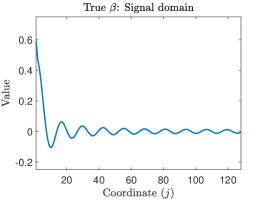
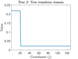
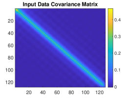
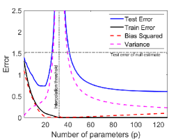
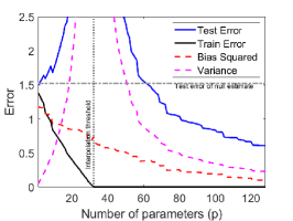
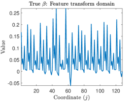
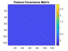
Figure 2: Empirical results for LS regression based on a class $\mathcal{F}_{p}^{\sf lin}(\{\mathbf{u}_{j}\}_{j=1}^{d})$ of linear functions in the form described in Example 2.1. The data model is ${y=\mathbf{x}^{T}\boldsymbol{\beta}+\epsilon}$. (a) The components of $\boldsymbol{\beta}$. (b) The components of the DCT transform of $\boldsymbol{\beta}$, i.e., $\mathbf{C}_{d}\boldsymbol{\beta}$. This shows that the majority of $\boldsymbol{\beta}$’s energy is at the low-range DCT “feature band” of $j=1,\dots,20$. (c) The input data covariance matrix $\mathbf{\Sigma}_{\mathbf{x}}$. As explained in detail in the main text, the second row of subfigures correspond to $\mathcal{F}_{p}^{\sf lin}(\{\mathbf{u}_{j}\}_{j=1}^{d})$ with DCT features, and the third row of subfigures correspond to $\mathcal{F}_{p}^{\sf lin}(\{\mathbf{u}_{j}\}_{j=1}^{d})$ with Hadamard features.

[] [] []
[] [] []

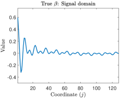
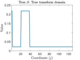
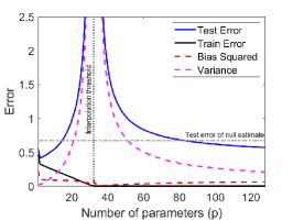
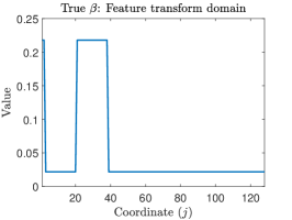
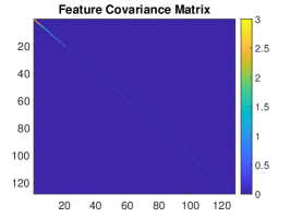
Figure 3: Empirical results for LS regression based on a class $\mathcal{F}_{p}^{\sf lin}(\{\mathbf{u}_{j}\}_{j=1}^{d})$ of linear functions in the form described in Example 2.1. The data model is ${y=\mathbf{x}^{T}\boldsymbol{\beta}+\epsilon}$. (a) The components of $\boldsymbol{\beta}$. (b) The components of the DCT transform of $\boldsymbol{\beta}$, i.e., $\mathbf{C}_{d}\boldsymbol{\beta}$. This shows that besides two high-energy components at the first two features, the majority of $\boldsymbol{\beta}$’s energy is at the mid-range DCT “feature band” of $j=21,\dots,38$. (c) The input data covariance matrix $\mathbf{\Sigma}_{\mathbf{x}}$. As explained in detail in the main text, the second row of subfigures correspond to $\mathcal{F}_{p}^{\sf lin}(\{\mathbf{u}_{j}\}_{j=1}^{d})$ with DCT features.

2.3 Why is double descent a surprise?

As a consequence of the classical bias-variance tradeoff, the test error as a function of the number of parameters forms a U-shaped curve in the underparameterized regime. For example, Fig. 2 depicts this U-shaped curve in the underparameterized range of solutions $p<n$, i.e., to the left of the interpolation threshold (vertical dotted line at $p=n=32$). This classical bias-variance tradeoff is usually induced by two fundamental behaviors of non-interpolating solutions:

• The bias term usually decreases because the optimal mapping $f_{\sf opt}$ can be better approximated by classes of mappings $\mathcal{F}$ that are more complex. In other words, models with more parameters or less regularization typically result in a lower (squared) bias component in the test error decomposition (7). As an example, see the red dashed curve to the left of the interpolation threshold in Fig. 2.

• The variance term usually increases because classes of mapping $\mathcal{F}$ that are of higher complexity result in higher sensitivity to (or variation with respect to) the noise in the specific training dataset $\mathcal{D}$. Note that such noise can arise due to stochastic measurement errors and/or model misspecification (see, e.g., Rao, 1971). In other words, models with more parameters or less regularization typically result in a higher variance component in the test error decomposition (7). As an example, see the magenta dashed curve to the left of the interpolation threshold in Fig. 2.

Typically, the interpolating solution of minimal complexity (e.g., $\mathcal{F}_{p}^{\sf lin}(\{\mathbf{u}_{j}\}_{j=1}^{d})$ for $p=n$) has a high test error due to a high variance term around the transition between non-interpolating and interpolating regimes. This inferior performance at the entrance to the interpolation threshold (which can be mathematically explained through poor conditioning of the training data matrix) led to a neglect of the study of the range of interpolating solutions, i.e., models such as Examples 2.1-2.2 with $p>n$. However, the recently observed success of interpolation and overparameterization across deep learning (Neyshabur et al., 2014; Zhang et al., 2017; Advani et al., 2020) and simpler models like linear models and shallow neural networks (Spigler et al., 2019; Belkin et al., 2019a; Geiger et al., 2020) alike has changed this picture; the interpolating/overparameterized regime is now actively researched. It is essential to note that we cannot expect double descent behavior to arise from any interpolating solution; indeed, it is easy to find solutions that would generalize poorly even as more parameters are added. Accordingly, we should expect the implicit regularization present in the minimum $\ell_{2}$-norm interpolation to play a critical role in aiding generalization. However, implicit regularization constitutes a sanity check rather than a full explanation for the double descent behavior. For one, it does not explain the seemingly harmless interpolation of noise in training data in the highly overparameterized regime. For another, minimum $\ell_{2}$-norm interpolations will not generalize well for any data distribution: indeed, classic experiments demonstrate catastrophic signal reconstruction in some cases by the minimum $\ell_{2}$-norm interpolation (Chen et al., 2001). An initial examination of the bias-variance decomposition of test error in the interpolating regime (Figures 2,2 and 3) demonstrates significantly different behavior from the underparameterized regime, at least when minimum $\ell_{2}$-norm solutions are used: there appears to be a significant decrease in the variance component that dominates the increase in the bias component to cause an overall benefit in overparameterization. It is also unclear whether the interpolating regime is strictly beneficial for generalization in the sense that the global minimum of the test error is achieved by an interpolating solution. The simple experiments in this section demonstrate a mixed answer to this question: Figs. 2 and 2 demonstrate beneficial double descent behaviors, whereas Fig. 3 shows a double descent behavior but the underparameterized regime is the one that minimizes test error.

2.4 The role of model misspecification in beneficial interpolation

Misspecification was defined above as a learning setting where the function class $\mathcal{F}$ does not include the optimal solution $f_{\sf opt}$ that minimizes the test error. In this section, we provide an elementary calculation to illustrate that this model misspecification is a significant ingredient in inducing the double descent behavior. Consider regression with respect to squared error loss, data model ${y=\mathbf{x}^{T}\boldsymbol{\beta}+\epsilon}$ and a function class ${\mathcal{F}_{p}^{\sf lin}(\{\mathbf{u}_{j}\}_{j=1}^{d})}$ as in Example 2.1. Then, the optimal solution is ${f_{\sf opt}(\mathbf{x})=\mathbb{E}\left[{{y|\mathbf{x}}}\right]=\mathbf{x}^{T}\boldsymbol{\beta}}$. By the definition of the function class ${\mathcal{F}_{p}^{\sf lin}(\{\mathbf{u}_{j}\}_{j=1}^{d})}$, the learned mapping is applied on a feature vector $\boldsymbol{\phi}=\mathbf{U}_{p}^{T}\mathbf{x}$ that includes only $p$ features (out of the $d$ possible features) of the input $\mathbf{x}$. This means that the optimal solution in the function class ${\mathcal{F}_{p}^{\sf lin}(\{\mathbf{u}_{j}\}_{j=1}^{d})}$ is

$$f_{{\sf opt},\mathcal{F}_{p}^{\sf lin}}(\mathbf{x})=\mathbb{E}\left[{{y|\boldsymbol{\phi}}}\right]=\boldsymbol{\phi}^{T}\mathbf{U}_{p}^{T}\boldsymbol{\beta}=\mathbf{x}^{T}\mathbf{U}_{p}\mathbf{U}_{p}^{T}\boldsymbol{\beta}$$ (17)

where the second equality is due to the orthogonality of the basis vectors $\{\mathbf{u}_{j}\}_{j=1}^{d}$. We can notice the difference between the optimal solution $f_{{\sf opt},\mathcal{F}_{p}^{\sf lin}}$ in ${\mathcal{F}_{p}^{\sf lin}(\{\mathbf{u}_{j}\}_{j=1}^{d})}$ and the unconstrained optimal solution $f_{\sf opt}$ as follows. Note that $\mathbf{U}_{p}\mathbf{U}_{p}^{T}$ in (17) is the projection matrix onto the $p$-dimensional feature space that is utilized for learning and spanned by the $p$ orthonormal vectors $\{\mathbf{u}_{j}\}_{j=1}^{p}$. Hence, unless both $\boldsymbol{\beta}$ and the entire distribution of $\mathbf{x}$ are contained in the $p$-dimensional feature space, there is misspecification that excludes the optimal solution $f_{\sf opt}$ from the function class ${\mathcal{F}_{p}^{\sf lin}(\{\mathbf{u}_{j}\}_{j=1}^{d})}$.

Consider cases where the features are statistically independent (e.g., the above example with DCT features and Gaussian input with covariance matrix that is diagonalized by the DCT matrix). These cases let us to further emphasize the effect of misspecification on the bias and variance of the learned solution from ${\mathcal{F}_{p}^{\sf lin}(\{\mathbf{u}_{j}\}_{j=1}^{d})}$. The important observation here is that the data model ${y=\mathbf{x}^{T}\boldsymbol{\beta}+\epsilon}$ can be written as

$$y=\boldsymbol{\phi}^{T}\mathbf{U}_{p}^{T}\boldsymbol{\beta}+\xi+\epsilon$$ (18)

where $\boldsymbol{\phi}=\mathbf{U}_{p}^{T}\mathbf{x}$ is the $p$-dimensional feature vector of the input, and ${\xi\triangleq\sum_{j=p+1}^{d}{\left(\mathbf{u}_{j}^{T}\mathbf{x}\right)\left(\mathbf{u}_{j}^{T}\boldsymbol{\beta}\right)}}$ is a random variable which is statistically independent of the feature vector $\boldsymbol{\phi}$. We consider zero-mean Gaussian input $\mathbf{x}$, here, with covariance matrix ${\mathbf{\Sigma}_{\mathbf{x}}=\mathbf{U}\mathbf{\Lambda}_{\mathbf{x}}\mathbf{U}^{T}}$. Hence, the misspecification variable $\xi$ is also zero-mean Gaussian but with variance

$$\sigma_{\xi}^{2}=\sum_{j=p+1}^{d}{\lambda_{j}\cdot\left(\mathbf{u}_{j}^{T}\boldsymbol{\beta}\right)^{2}},$$ (19)

which sums over the $d-p$ feature directions that are not utilized in the $p$-dimensional feature space of ${\mathcal{F}_{p}^{\sf lin}(\{\mathbf{u}_{j}\}_{j=1}^{d})}$.

We define the misspecification bias (squared) as

$${\sf bias}_{\sf misspec}^{2}\left(\widehat{f}\right)\triangleq\mathbb{E}_{\mathbf{x}}\left[{{\left(f_{{\sf opt},\mathcal{F}_{p}^{\sf lin}}(\mathbf{x})-f_{\sf opt}(\mathbf{x})\right)^{2}}}\right],$$ (20)

namely, the expected squared difference between the optimal solution in the function class ${\mathcal{F}_{p}^{\sf lin}(\{\mathbf{u}_{j}\}_{j=1}^{d})}$ and the optimal unconstrained solution. We also define the in-class bias (squared) as

$${\sf bias}_{\sf inclass}^{2}\left(\widehat{f}\right)\triangleq\mathbb{E}_{\mathbf{x}}\left[{{\left(\mathbb{E}_{\mathcal{D}}\left[{{\widehat{f}(\mathbf{x})}}\right]-f_{{\sf opt},\mathcal{F}_{p}^{\sf lin}}(\mathbf{x})\right)^{2}}}\right],$$ (21)

which is the expected squared difference between the learned solution (expected over the training dataset) and the optimal solution in the function class ${\mathcal{F}_{p}^{\sf lin}(\{\mathbf{u}_{j}\}_{j=1}^{d})}$ that was utilized for learning. Now, based on the orthogonality of the feature maps that form ${\mathcal{F}_{p}^{\sf lin}(\{\mathbf{u}_{j}\}_{j=1}^{d})}$ and considering cases where the features are statistically independent, we can decompose the squared bias from (8) as

$${\sf bias}^{2}\left(\widehat{f}\right)={\sf bias}_{\sf misspec}^{2}\left(\widehat{f}\right)+{\sf bias}_{\sf inclass}^{2}\left(\widehat{f}\right),$$ (22)

which can be further set in the test error decomposition in (7). More specifically, the definition of ${\mathcal{F}_{p}^{\sf lin}(\{\mathbf{u}_{j}\}_{j=1}^{d})}$ in Example 2.1 implies that

$${\sf bias}_{\sf misspec}^{2}\left(\widehat{f}\right)=\sigma_{\xi}^{2},$$ (23)

which is the variance (19) of the misspecification variable $\xi$.

Still considering statistically independent features, we can also decompose the variance term (9) to express its portion due to misspecification in ${\mathcal{F}_{p}^{\sf lin}(\{\mathbf{u}_{j}\}_{j=1}^{d})}$. We can write the variance decomposition as

$${\sf var}\left(\widehat{f}\right)={\sf var}_{\sf misspec}\left(\widehat{f}\right)+{\sf var}_{\sf inclass}\left(\widehat{f}\right).$$ (24)

Here, the variance component due to misspecification is

$${\sf var}_{\sf misspec}\left(\widehat{f}\right)=\sigma_{\xi}^{2}\operatorname{Tr}\left\{{\mathbf{\Lambda}_{\mathbf{x},p\times p}\mathbb{E}_{\mathbf{\Phi}}\left[{{\mathbf{\Phi}^{+}\mathbf{\Phi}^{+,T}}}\right]}\right\}$$ (25)

where $\mathbf{\Phi}=\mathbf{X}\mathbf{U}_{p}$ is the $n\times p$ matrix of training input features, and $\mathbf{\Lambda}_{\mathbf{x},p\times p}$ is the $p\times p$ diagonal matrix with input covariance eigenvalues $\lambda_{1},\dots,\lambda_{p}$. The in-class variance component ${\sf var}_{\sf inclass}(\widehat{f})$ has a bit more intricate formulation that we exclude from this discussion. Hastie et al. (2019) further assume that the input and the true parameter vector are both isotropic random vectors and, accordingly, provide a simple formulation for the in-class variance term in their setting.

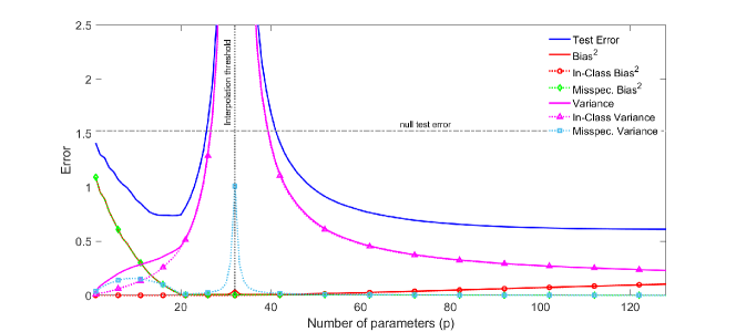
Figure 4: Bias-variance decomposition of test error, including further decomposition into misspecification and in-class components as formulated in (22)-(25) for cases with statistically independent features. This figure is an extension of Fig. 2. These results are for LS regression with DCT features and Gaussian input with covariance that is diagonlized by the DCT matrix.

Let us return to the example given in Fig. 2 for regression with DCT features that are statistically independent due to the covariance form of the Gaussian input. This setting allows us to demonstrate the misspecification components of the bias and variance from (23) and (25). Figure 4 extends Fig. 2 by illustrating the misspecification and in-sample components of the bias and variance versus the number of parameters $p$ in the function class. Indeed, the misspecification bias decreases as the function class is more parameterized. In contrast, the in-class bias is zero in the underparameterized regime, and increases with $p$ in the overparameterized regime. Yet, the reduction in the misspecification bias due to overparameterization is more significant than the corresponding increase in the in-sample bias; and this is in accordance with having the global minimum of test error in the overparameterized range. We can observe that both the in-class and misspecification variance terms peak around the interpolation threshold (i.e., $p=n$) due to the poor conditioning of the input feature matrix. Based on the structure of the true parameter vector (see Fig. 2), the significant misspecification occurs for $p<20$ and this is apparent for the misspecification components of both the bias and variance.

More generally than the case of statistically independent features, the examples in Figures 2-3 include misspecification for any $p<d$. This is because, for both DCT and Hadamard features, the representation of the true parameter vector $\boldsymbol{\beta}$ requires all the $d$ features (see Figures 2,2,3). Learning using DCT features benefits from the fact that $\boldsymbol{\beta}$ has energy compaction in the DCT domain, which in turn significantly reduces the misspecification bias for $p$ that is large enough to include the majority of $\boldsymbol{\beta}$’s energy. In contrast, in the case of learning using the Hadamard features, the representation of $\boldsymbol{\beta}$ in the feature space has its energy spread randomly all over the features, without energy compaction, and therefore the effect of misspecification is further amplified in this case. The amplified misspecification due to a poor selection of feature space actually promotes increased benefits from overparameterization (compared to underparameterized solutions, which are extremely misspecified) as can be observed in Fig. 2.

The in-depth experiments and explanation above illustrate the rich variety of generalization behaviors even in elementary settings. Understanding these behaviors requires mathematical study beyond the fundamental discussion in this section. In the next section, we review recently conducted mathematical studies on this topic, and illuminate the core phenomena that explain generalization behavior in this interpolating regime.

3 Overparameterized regression

Precise theoretical explanations now exist for the phenomena of harmless interpolation of noise and double descent (Belkin et al., 2020; Bartlett et al., 2020; Hastie et al., 2019; Kobak et al., 2020; Muthukumar et al., 2020b; Mitra, 2019). In this section, we provide a brief recap of these results, all focused on minimum $\ell_{2}$-norm interpolators. Additionally, we provide intuitive explanations for the double descent behavior in simplified toy settings that are inspired by statistical signal processing. We will see that the test error can be upper bounded by an additive decomposition of two terms:

• A signal-dependent term, which expresses how much error is incurred by a solution that interpolates the noiseless version of our (noisy) training data.

• A noise-dependent term, which expresses how much error is incurred by a solution that interpolates only the noise in our training data.

Situations that adequately tradeoff these terms give rise to the double descent behavior, and can be described succinctly for several families of linear models. We will now describe these results in more detail.

3.1 Summary of results

The minimum $\ell_{2}$-norm interpolator (MNI), denoted by the $p$-dimensional vector $\widehat{\boldsymbol{\alpha}}$ where $p>n$, has a closed-form expression (recall Eq. (16)). In turn, this allows to derive closed-form exact expressions for the generalization error as a function of the training dataset; indeed, all aforementioned theoretical analyses of the minimum $\ell_{2}$-norm interpolator take this route.

We can state the diversity of results by Belkin et al. (2020); Bartlett et al. (2020); Hastie et al. (2019); Kobak et al. (2020); Muthukumar et al. (2020b); Mitra (2019) in a common framework by decomposing the test error incurred by the MNI, denoted by $\widehat{\boldsymbol{\alpha}}$, into the respective test errors that would be induced by two related solutions. To see this, consider the noisy data model (2) with scalar output, and note that the MNI from (16) satisfies $\widehat{\boldsymbol{\alpha}}=\widehat{\boldsymbol{\alpha}}_{\sf{sig}}+\widehat{\boldsymbol{\alpha}}_{\sf{noise}}$ where

• $\widehat{\boldsymbol{\alpha}}_{\sf{sig}}\triangleq\mathbf{\Phi}^{+}\left({\mathbf{y}-\boldsymbol{\epsilon}}\right)$ is the minimum $\ell_{2}$-norm interpolator on the noiseless training dataset ${\mathcal{D}_{\sf{sig}}=\{(\mathbf{x}_{i},f_{\sf true}(\mathbf{x}_{i}))\}_{i=1}^{n}}$. Note that ${[f_{\sf true}(\mathbf{x}_{1}),\dots,f_{\sf true}(\mathbf{x}_{n})]^{T}=\mathbf{y}-\boldsymbol{\epsilon}\in\mathbb{R}^{n}}$, where the vectors $\mathbf{y},\boldsymbol{\epsilon}\in\mathbb{R}^{n}$ include the training data outputs and their error components, respectively.

• $\widehat{\boldsymbol{\alpha}}_{\sf{noise}}\triangleq\mathbf{\Phi}^{+}\boldsymbol{\epsilon}$ is the minimum $\ell_{2}$-norm interpolator on the pure noise ${\boldsymbol{\epsilon}\in\mathbb{R}^{n}}$ in the training data. In other words, $\widehat{\boldsymbol{\alpha}}_{\sf{noise}}$ is the minimum $\ell_{2}$-norm interpolator of the dataset ${\mathcal{D}_{\sf{noise}}=\{(\mathbf{x}_{i},\epsilon_{i})\}_{i=1}^{n}}$.

Then, a typical decomposition of an upper bound on the test error is given by

$${\mathcal{E}_{\sf test}}\leq{\mathcal{E}_{\sf test,sig}}+{\mathcal{E}_{\sf test,noise}},$$ (26)

where ${\mathcal{E}_{\sf test,sig}}$ is a signal specific component that is determined by the noiseless data interpolator $\widehat{\boldsymbol{\alpha}}_{\sf{sig}}$; and ${\mathcal{E}_{\sf test,noise}}$ is a noise specific component that is determined by the pure noise interpolator $\widehat{\boldsymbol{\alpha}}_{\sf{noise}}$. Moreover, we can typically lower bound the test error as ${\mathcal{E}_{\sf test}}\geq\max\{{\mathcal{E}_{\sf test,sig}},{\mathcal{E}_{\sf test,noise}}\}$; therefore, this decomposition is sharp in a certain sense.

All of the recent results on minimum $\ell_{2}$-norm interpolation can be viewed from the perspective of (26) such that they provide precise characterizations for the error terms ${\mathcal{E}_{\sf test,sig}}$ and ${\mathcal{E}_{\sf test,noise}}$ under the linear model, i.e., ${f_{\sf true}(\mathbf{x})=\mathbf{x}^{T}\boldsymbol{\beta}}$ for some ${\boldsymbol{\beta}\in\mathbb{R}^{d}}$. Moreover, as we will see, these analytical results demonstrate that the goals of minimizing ${\mathcal{E}_{\sf test,sig}}$ and ${\mathcal{E}_{\sf test,noise}}$ can sometimes be at odds with one another. Accordingly, the number of samples $n$, the number of parameters $p>n$, and properties of the feature covariance matrix $\mathbf{\Sigma}_{\boldsymbol{\phi}}$ should be chosen to tradeoff these error terms. In some studies, the ensuing error bounds are non-asymptotic and can be stated as a closed-form function of these quantities. In other studies, the parameters $p$ and $n$ are grown together at a fixed rate and the asymptotic test error is exactly characterized as a solution to either linear or nonlinear equations that is sometimes closed form, but at the very least typically numerically evaluatable. Such exact characterizations of the test error are typically called precise asymptotics.

For simplicity, we summarize recent results from the literature in the non-asymptotic setting, i.e., error bounds that hold for finite values of $n$,$p$ and $d$ (in addition to their infinite counterparts). Accordingly, we characterize the behavior of the test error (and various factors influencing it) as a function of the parameters $n,p,d$ using two types of notation. First, considering an arbitrary function $h(\cdot,\cdot,\cdot)$, we will use ${{\mathcal{E}_{\sf test}}=\mathcal{O}(h(n,p,d))}$ to mean that there exists a universal constant $C>0$ such that ${\mathcal{E}_{\sf test}}\leq Ch(n,p,d)$ for all $n,p,d$. Second, we will use ${\mathcal{E}_{\sf test}}=\Theta(h(n,p,d))$ to mean that there exist universal constants ${c,C>0}$ such that ${ch(n,p,d)\leq{\mathcal{E}_{\sf test}}\leq Ch(n,p,d)}$ for all $n,p,d$. Moreover, the bounds that we state typically hold with high probability over the training data, in the sense that the probability that the upper bound holds goes to $1$ as $n\to\infty$ (and $p,d\to\infty$ with the desired proportions with respect to $n$ in order to maintain overparameterization).

3.1.1 When does the minimum $\ell_{2}$-norm solution enable harmless interpolation of noise?

We begin by focusing on the contribution to the upper bound on the test error that arises from a fit of pure noise, i.e., ${\mathcal{E}_{\sf test,noise}}$, and identifying necessary and sufficient conditions under which this error is sufficiently small. We will see that these conditions, in all cases, reduce to a form of high “effective overparameterization” in the data relative to the number of training examples (in a sense that we will define shortly). In particular, these results can be described under the following two particular models for the feature covariance matrix $\mathbf{\Sigma}_{\boldsymbol{\phi}}$:

1. The simplest result to obtain is in the case of isotropic covariance, for which $\mathbf{\Sigma}_{\boldsymbol{\phi}}=\mathbf{I}_{p}$. For instance, this case occurs when the feature maps in Example 2.1 are applied on input data $\mathbf{x}$ with isotropic covariance matrix $\mathbf{\Sigma}_{\mathbf{x}}=\mathbf{I}_{d}$. If the features are also statistically independent (e.g., consider Example 2.1 with isotropic Gaussian input data), the results by Bartlett et al. (2020); Hastie et al. (2019); Muthukumar et al. (2020b) imply that the noise error term scales as

   $${\mathcal{E}_{\sf test,noise}}=\Theta\left(\frac{\sigma_{\epsilon}^{2}n}{p}\right)$$ (27)

   where $\sigma_{\epsilon}^{2}$ denotes the noise variance. The result in (27) displays an explicit benefit of overparameterization in fitting noise in a harmless manner. In more detail, this result is (i) a special case of the more general (non-asymptotic) results for arbitrary covariance by Bartlett et al. (2020), (ii) one of the closed-form precise asymptotic results presented as $n,p\to\infty$ by Hastie et al. (2019), and (iii) a consequence of the more general characterization of the minimum-risk interpolating solution, or “ideal interpolator”, derived by Muthukumar et al. (2020b).

   On the other hand, the signal error term can be bounded as

   $${\mathcal{E}_{\sf test,sig}}=\Theta\left(||\boldsymbol{\beta}||_{2}^{2}\left(1-\frac{n}{p}\right)\right),$$ (28)

   displaying an explicit harm in overparameterization from the point of view of signal recovery. In more detail, this result is (i) a non-asymptotic upper bound provided by Bartlett et al. (2020) (and subsequent work by Tsigler and Bartlett (2020) shows that this term is matched by a sharp lower bound), (ii) precise asymptotics provided by Hastie et al. (2019).

   As discussed later in Section 3.1.2, the behavior of ${\mathcal{E}_{\sf test,sig}}$ has negative implications for consistency in a certain high-dimensional sense. Nevertheless, the non-asymptotic example in Figure 5 shows that one can construct signal models with isotropic covariance that can benefit from overparameterization. Such benefits are partly due to the harmless interpolation of noise, and partly due to a decrease in the misspecification error arising from increased overparameterization.

2. The general case of anisotropic covariance and features that are independent in their principal component basis is significantly more complicated. Nevertheless, it turns out that a high amount of “effective overparameterization” can be defined, formalized, and shown to be sufficient and necessary for interpolating noise in a harmless manner. This formalization was pioneered by Bartlett et al. (2020), who provide a definition of effective overparameterization solely as a function of $n$, $p$ and the spectrum of the covariance matrix $\mathbf{\Sigma}_{\boldsymbol{\phi}}$, denoted by the eigenvalues ${\lambda_{1}\geq\ldots\geq\lambda_{p}}$. We refer the reader to Bartlett et al. (2021) for a detailed exposition of these results and their consequences. Here, we present the essence of these results in a popular model used in high-dimensional statistics, the spiked covariance model. Under this model (recall that $p>n$), we have a feature covariance matrix $\mathbf{\Sigma}_{\boldsymbol{\phi}}$ with ${s<p-n}$ high-energy eigenvalues and ${p-s}$ low-energy (but non-zero) eigenvalues. In other words, ${\lambda_{1}\geq\ldots\geq\lambda_{s}=\lambda_{H}}$ and ${\lambda_{s+1}=\ldots=\lambda_{p}=\lambda_{L}}$ for some ${\lambda_{H}\gg\lambda_{L}}$ (for example, notice that Figure 2 is an instance of this model). In this special case, the results of Bartlett et al. (2020) can be simplified to show that the test error arising from overfitting noise is given by

   $${\mathcal{E}_{\sf test,noise}}=\Theta\left(\sigma_{\epsilon}^{2}\left(\frac{s}{n}+\frac{n}{p-s}\right)\right).$$ (29)

   Equation (29) demonstrates a remarkably simple set of sufficient and necessary conditions for harmless interpolation of noise in this anisotropic ensemble:

   • The number of high-energy directions, given by $s$, must be significantly smaller than the number of samples $n$.

   • The number of low-energy directions, given by $p-s$, must be significantly larger than the number of samples $n$. This represents a requirement for sufficiently high “effective overparameterization” to be able to absorb the noise in the data, and fit it in a relatively harmless manner.

Interestingly, the work of Kobak et al. (2020) considered the above anisotropic model for the special case of a single spike (i.e., for $s=1$, which usually implies that the first condition is trivially met) and showed that the error incurred by interpolation is comparable to the error incurred by ridge regression. These results are related in spirit to the above framework, and so we can view the conditions derived by Bartlett et al. (2020) as sufficient and necessary for ensuring that interpolation of (noisy) training data does not lead to sizably worse performance than ridge regression. Of course, good generalization of ridge regression itself is not always a given (in particular, it generalizes poorly for isotropic models). In this vein, the central utility of studying this anisotropic case is that it is now possible to also identify situations under which the test error arising from fitting pure signal, i.e., ${\mathcal{E}_{\sf test,sig}}$, is sufficiently small. We elaborate on this point next.

[] [] []
[] [] []

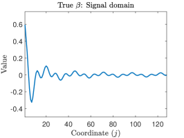
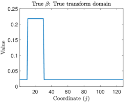
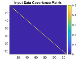
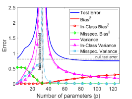
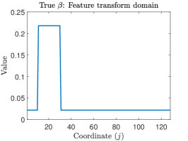
Figure 5: Empirical results for LS regression based on a class $\mathcal{F}_{p}^{\sf lin}(\{\mathbf{u}_{j}\}_{j=1}^{d})$ of linear functions in the form described in Example 2.1. The data model is ${y=\mathbf{x}^{T}\boldsymbol{\beta}+\epsilon}$. (a) The components of $\boldsymbol{\beta}$. (b) The components of the DCT transform of $\boldsymbol{\beta}$, i.e., $\mathbf{C}_{d}\boldsymbol{\beta}$. This shows that the majority of $\boldsymbol{\beta}$’s energy is at the DCT “feature band” of $j=11,\dots,30$. (c) The input data covariance matrix $\mathbf{\Sigma}_{\mathbf{x}}$. The learning is done using DCT features and, accordingly, the features are independent and isotropic due to the isotropic Gaussian input. Subfigure (d) shows the test error (as a function of $p$) and its decomposition to bias, variance, and their in-class and misspecification components.

3.1.2 When does the minimum $\ell_{2}$-norm solution enable signal recovery?

The above results paint a compelling picture for an explicit benefit of overparameterization in harmless interpolation of noise (via minimum $\ell_{2}$-norm interpolation). However, good generalization requires the term ${\mathcal{E}_{\sf test,sig}}$ to be sufficiently small as well. As we now demonstrate, the picture is significantly more mixed for signal recovery.

As shown in Eq. (28), for the case of isotropic covariance, the signal error term ${\mathcal{E}_{\sf test,sig}}$ can be upper and lower bounded upto universal constants as $||\boldsymbol{\beta}||_{2}^{2}\left(1-\frac{n}{p}\right)$, displaying an explicit harm in overparameterization from the point of view of signal recovery. The ills of overparameterization in signal recovery with the minimum $\ell_{2}$-norm interpolator are classically documented in statistical signal processing; see, e.g., the experiments in the seminal survey by Chen et al. (2001). A fundamental consequence of this adverse signal recovery is that the minimum $\ell_{2}$-norm interpolator cannot have statistical consistency (i.e., we cannot have ${\mathcal{E}_{\sf test}}\to 0$ as $n\to\infty$) under isotropic covariance for any scaling of $p$ that grows with $n$, whether constant (i.e., $p=\gamma n$ for some fixed $\gamma>1$), or ultra high dimensional (i.e., $p=n^{q}$ for some $q>1$). Instead, the test error converges to the “null risk”, i.e., the test error that would be induced by the “zero-fit” $\widehat{\boldsymbol{\alpha}}_{0}:=\mathbf{0}$.

These negative results make clear that anisotropy of features is required for the signal-specific error term ${\mathcal{E}_{\sf test,sig}}$ to be sufficiently small; in fact, this is the main reason for the requirement that $\lambda_{H}\gg\lambda_{L}$ in the spiked covariance model to ensure good generalization in regression tasks. In addition to this effective low dimensionality in data, we also require a low-dimensional assumption on the signal model. In particular, the signal energy must be almost entirely aligned with the directions (i.e., eigenvectors) of the top $s\ll n$ eigenvalues of the feature covariance matrix (representing high-energy directions in the data). Finally, we note as a matter of detail that the original work by Bartlett et al. (2020) precisely characterizes the contribution from ${\mathcal{E}_{\sf test,noise}}$ upto constants independent of $p$ and $n$; however, they only provide upper bounds on the bias term. In follow-up work, Tsigler and Bartlett (2020) provide more precise expressions for the bias that show that the bias is non-vanishing in “tail” signal components outside the first $s$ “preferred” directions. Their upper and lower bounds match up to a certain condition number. The follow-up studies by Mei and Montanari (2019); Liao et al. (2020); Derezinski et al. (2020); Mei et al. (2021) also provide precise asymptotics for the bias and variance terms in very general random feature models, which can be shown to fall under the category of anisotropic covariance models.

3.1.3 When does double descent occur?

The above subsections show that the following conditions are sufficient and necessary for good generalization of the minimum $\ell_{2}$-norm interpolator:

• low-dimensional signal structure, with the non-zero components of the signal aligned with the $s$ eigenvectors corresponding to the highest-value eigenvalues (i.e., high-energy directions in the data)

• low effective dimension in data

• an overparameterized number of low-value (but non-zero) directions.

Given these pieces, the ingredients for double descent become clear. In addition to the aforementioned signal and noise-oriented error terms in (26), we will in general have a misspecification error term, denoted by ${\mathcal{E}_{\sf test,missp}}$, which will always decrease with overparameterization and therefore further contributes to the double descent phenomenon. For example, recall Section 2.4 and the example in Fig. 4 where the misspecification bias and variance terms decrease with $p$ in the overparameterized range. Optimization aspects can also affect the double descent behavior, for example, D’Ascoli et al. (2020) study the contribution of optimization initialization to double descent phenomena in a lazy training setting (i.e., where the learned parameters are close to their initializations (Chizat et al., 2019)).

Examples of the approximation-theoretic benefits of overparameterization are also provided by Hastie et al. (2019), but these do not go far enough to recover the double descent behavior, as they are still restricted to the isotropic setting in which signal recovery becomes more harmful as the number of parameters increases. Belkin et al. (2020) provided one of the first explicit characterizations of double descent under two models of randomly selected “weak features”. In their model, the $p$ features are selected uniformly at random from an ensemble of $d$ features (which are themselves isotropic in distribution and follow either a Gaussian or Fourier model). This idea of “weak features” is spiritually connected to the classically observed benefits of overparameterization in ensemble models like random forests and boosting, which were recently discussed in an insightful unified manner (Wyner et al., 2017). This connection was first mentioned in Belkin et al. (2019a).

Subsequent to the first theoretical works on this topic, Mei and Montanari (2019) also showed precise asymptotic characterizations of the double descent behavior in a random features model.

3.2 A signal processing perspective on harmless interpolation

In this section, we present an elementary explanation for harmless interpolation using the concepts of aliasing and Parseval’s theorem for a “toy” case of overparameterized linear regression with cosine features on regularly spaced, one-dimensional input data. This elementary explanation was first introduced by Muthukumar et al. (2020b), and inspired subsequent work for the case of classification (Muthukumar et al., 2020a). While this calculation illuminates the impact of interpolation in both isotropic and anisotropic settings, we focus here on the isotropic case for simplicity.

This toy setting can be perceived as a special case of Example 2.2 with one-dimensional input and cosine feature maps. Note that our example for real-valued cosine feature maps differs in some low-level mathematical details compared to the analysis originally given by Muthukumar et al. (2020b) for Fourier features.

Example 3.1 (Cosine features for one-dimensional input).

Throughout this example, we will consider $p$ to be an integer multiple of $n$. We also consider one-dimensional data $x\in[0,1]$ and a family of cosine feature maps ${\varphi_{j}(x)=\kappa_{j}\cos((j-1)\pi x),~{}j=1,\dots,\infty}$, where the normalization constant $\kappa_{j}$ equals $1$ for $j=1$ and $\sqrt{2}$ for $j\geq 2$. Then, the $p$-dimensional cosine feature vector is given by

$$\phi(x)=\begin{bmatrix}1&\sqrt{2}\cos(\pi x)&\sqrt{2}\cos(\pi(2x))&\ldots&\sqrt{2}\cos(\pi(p-1)x)\end{bmatrix}^{T}\in\mathbb{R}^{p}.$$

This is clearly an orthonormal, i.e., isotropic feature family in the sense that

$$\mathbb{E}_{x\sim\text{Unif}[0,1]}\left[\varphi_{j}(x)\varphi_{k}(x)\right]=\int_{x\in[0,1]}\varphi_{j}(x)\varphi_{k}(x)dx=\delta_{jk},$$

where $\delta_{jk}$ denotes the Kronecker delta. Furthermore, in this “toy” model we assume $n$-regularly spaced training data points, i.e., ${x_{i}=\frac{i-\frac{1}{2}}{n}}\text{ for }i=1,\ldots,n$. While the more standard model in the ML setup would be to consider $\{x_{i}\}_{i=1}^{n}$ to be i.i.d. draws from the input distribution (which is uniform over $[0,1]$ in this example), the toy model with deterministic, regularly-spaced $\{x_{i}\}_{i=1}^{n}$ will yield a particularly elementary and insightful analysis owing to the presence of exact aliases.

In the regime of overparameterized learning, we have $p>n$. The case of regularly-spaced training inputs allows us to see overparameterized learning as reconstructing an undersampled signal: the number of samples (given by $n$) is much less than the number of features (given by $p$). Thus, the undersampling perspective implies that aliasing, in some approximate sense, is a core issue that underlies model behavior in overparameterized learning . We illustrate this through Example 3.1, which is an idealized toy model and a special case of Example 2.2.

Here, the true signal is of the form ${f_{\sf true}:[0,1]\rightarrow\mathbb{R}}$. Then, we have the noisy training data

$$y_{i}=f_{\sf true}(x_{i})+\epsilon_{i}\text{ for }i=1,\ldots,n,$$ (30)

where ${x_{i}=\frac{i-\frac{1}{2}}{n}}$. The overparameterized estimator has to reconstruct a signal over the continuous interval $[0,1]$ while interpolating the $n$ given data points using a linear combination of ${p>n}$ orthonormal cosine functions $\varphi_{j}(x)$, $j=1,\ldots,p$, that were defined in Example 3.1 for ${x\in[0,1]}$. In other words, various interpolating function estimates can be induced by plugging different parameters ${\{\alpha_{j}\}_{j=1}^{p}\in\mathbb{R}}$ in

$$f(x)=\sum_{j=1}^{p}{\alpha_{j}\varphi_{j}(x)}=\alpha_{1}+\sqrt{2}\sum_{j=2}^{p}{\alpha_{j}\cos\left((j-1)\pi x\right)}$$ (31)

such that $f(x_{i})=y_{i}$ for $i=1,\dots,n$. The assumed uniform distribution on the test input implies that the performance of an estimate $f$ is evaluated as ${\mathcal{E}_{\sf test}(f)=\sigma_{\epsilon}^{2}+\int_{x=0}^{1}{(f(x)-f_{\sf true}(x))^{2}dx}}$. In Figure 6 we demonstrate results in the setting of Example 3.1. Figure 6 illustrates the minimum $\ell_{2}$-norm solution of the form (31) for $p=24$ parameters. The training and test error curves (as a function of $p$) in Figure 6 show that the global minimum of test error is obtained in the overparameterized with $p=24$ parameters (there are $n=8$ training examples).

[] []

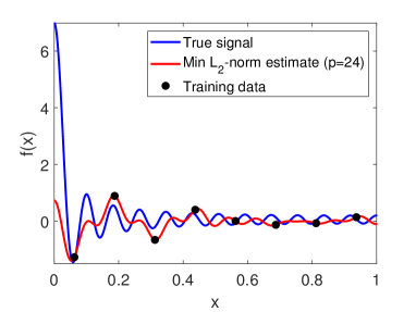
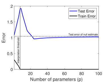
Figure 6: Evaluation of LS regression using orthonormal cosine features as in Example 3.1. The true signal is a linear combination of the first 25 cosine functions (see blue curve in (a)). The standard deviation of the noise is $\sigma=0.2$. The number of training data points is $n=8$. (a) Example of the minimum $\ell_{2}$-norm solution for $p=24$. (b) Test and training error curves for the min $\ell_{2}$-norm solutions with varying number of parameters $p$.

In the discussion below, we will consider (30) in both noisy and noiseless settings (where $\epsilon_{i}=0$ in the latter case). To demonstrate clearly the concept of aliasing, suppose the true signal is

$$f_{\sf true}(x)=\cos(k\pi x),$$ (32)

i.e., a single cosine function whose frequency is determined by an integer ${k\in\{1,\dots,n-1\}}$. We start by considering the noiseless version of (30), which we illustrate in Figure 7. (Note that in this figure the true signal and the training data points are presented as blue curve and black circle markers, respectively.) Then, a trivial estimate that interpolates all the training data points is the unnormalized $(k+1)^{\rm th}$ cosine function: ${f_{{\sf alias},0}(x)=\frac{1}{\sqrt{2}}\varphi_{k+1}(x)=\cos(k\pi x)}$. Yet, $f_{{\sf alias},0}(x)$ is not the only interpolating estimate that relies on a single cosine function. Recall that in Example 3.1 we assume $p/n$ to be an integer. Then, using periodicity and other basic properties of cosine functions, one can prove that there is a total of $N_{\sf alias}\triangleq\frac{p}{n}$ estimates (each in a form of a single cosine function from $\varphi_{j}(x)$, $j=1,\dots,p$) that interpolate the training data over the grid $x_{i}=\frac{i-\frac{1}{2}}{n}$, $i=1,\dots,n$. Specifically, one subset of single-cosine interpolating estimates is given by

$$f_{{\sf alias},\ell}(x)=\frac{(-1)^{\ell}}{\sqrt{2}}\varphi_{1+k+2\ell n}(x)=(-1)^{\ell}\cos((k+2\ell n)\pi x)\text{~{}~{}~{}for~{}}\ell=0,\dots,\left\lceil{\frac{N_{\sf alias}}{2}}\right\rceil-1,$$ (33)

and the second subset of single-cosine interpolating estimates is given by

$$f_{{\sf alias},-\ell}(x)=\frac{(-1)^{\ell}}{\sqrt{2}}\varphi_{1-k+2\ell n}(x)=(-1)^{\ell}\cos((-k+2\ell n)\pi x)\text{~{}~{}~{}for~{}}\ell=1,\dots,\left\lfloor{\frac{N_{\sf alias}}{2}}\right\rfloor.$$ (34)

One of these aliases is shown as the green curve (along with the true signal as the blue curve) in Figure 7. Clearly, the total number of such aliases, given by $N_{\sf alias}\triangleq\frac{p}{n}$, increases with overparameterization. Next, note that each of the interpolating aliases $f_{{\sf alias},\ell}(x)$, ${\ell=-\left\lfloor{\frac{N_{\sf alias}}{2}}\right\rfloor,\dots,0,\dots,\left\lceil{\frac{N_{\sf alias}}{2}}\right\rceil-1}$, is induced by setting a value of magnitude $\frac{1}{\sqrt{2}}$ to one of the $N_{\sf alias}$ relevant parameters in the estimate form (31). Accordingly, we will now see that none of these aliases is the minimum $\ell_{2}$-norm interpolating estimate (interestingly note that the interpolating estimate ${f_{{\sf alias},0}(x)=\cos(k\pi x)}$ is not of minimum $\ell_{2}$-norm even though this estimate coincides with the true signal $f_{{\sf true}}(x)$ for any $x\in[0,1]$). Indeed, the minimum $\ell_{2}$-norm solution $\widehat{\boldsymbol{\alpha}}$ in this noiseless case of a pure cosine function equally weights all of the exact aliases, and is expressed by the parameters

[] []

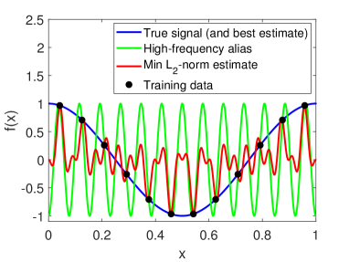
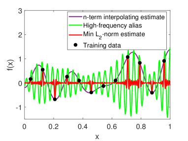
Figure 7: Illustration of aliasing and its effect on the minimum $\ell_{2}$-norm interpolator. Two idealized settings of Example 3.1 are shown. Left subfigure (a): A noiseless case ($\sigma=0$) where the true signal is ${f_{\sf true}(x)=\cos(2\pi x)}$ and the $n=12$ training data points are ${y_{i}=\cos(2\pi x_{i})}$ for ${i=1,\ldots,n}$. The trivial single-cosine alias, $f_{{\sf alias},0}(x)$ coincides with ${f_{\sf true}(x)}$ in the blue curve, a corresponding high-frequency alias $f_{{\sf alias},1}(x)$ is presented as the green curve. The minimum $\ell_{2}$-norm estimate for $p=48$ is presented as the red curve. Right subfigure (b):  A noisy case where the noise standard deviation is $\sigma=0.3$, the true signal is ${f_{\sf true}(x)=0}$, and the $n=12$ training data points are ${y_{i}=\epsilon_{i}}$ for ${i=1,\ldots,n}$. The interpolating estimate using the first $n$ cosine functions is presented as the purple curve, a high frequency alias of this estimate is presented as the green curve. The minimum $\ell_{2}$-norm estimate for $p=180$ is presented as the red curve.

$$\widehat{\alpha}_{j}=\begin{cases}\frac{(-1)^{\ell}}{N_{\sf alias}\sqrt{2}},&\text{for~{}~{}}j=1+k+2\ell n,~{}\ell=0,\dots,\left\lceil{\frac{N_{\sf alias}}{2}}\right\rceil-1\vspace{0.05in}\\ \frac{(-1)^{\ell}}{N_{\sf alias}\sqrt{2}},&\text{for~{}~{}}j=1-k+2\ell n,~{}\ell=1,\dots,\left\lfloor{\frac{N_{\sf alias}}{2}}\right\rfloor\\ 0,&\text{otherwise.}\end{cases}$$ (35)

Accordingly, the $\ell_{2}$-norm of $\widehat{\boldsymbol{\alpha}}$ is given by

$$\left\|{{\widehat{\boldsymbol{\alpha}}}}\right\|_{2}^{2}=N_{\sf alias}\left(\frac{1}{N_{\sf alias}\cdot\sqrt{2}}\right)^{2}=\frac{1}{2N_{\sf alias}}=\frac{n}{2p}.$$

Then, using Parseval’s theorem on the learned function form from (11) we get

$$\mathbb{E}\left[{{\left\|{{\widehat{f}(x)}}\right\|_{2}^{2}}}\right]=\mathbb{E}\left[{{\left\|{{\widehat{\boldsymbol{\alpha}}}}\right\|_{2}^{2}}}\right]=\frac{n}{2p},$$ (36)

also due to the definition of the cosine feature vector $\phi(x)$ in Example 3.1 that implies ${\mathbb{E}_{x}\left[{{\phi(x)\phi(x)^{T}}}\right]=\mathbf{I}_{p}}$. Note the minimum $\ell_{2}$-norm in (36) reduces as overparameterization increases. This behavior affects the corresponding test error and occurs also in more general cases where there is noise and the true signal is more complex than a single cosine function.

In Figure 7 we consider a “pure cosine” for the output (i.e., $f_{\sf true}$ is a single cosine function as in (30) but in a noiseless setting where $\epsilon_{i}=0$ for $i=1,\ldots,n$) to illustrate the exact orthogonal aliases clearly in (33)-(34). However, this aliasing effect would happen for arbitrary output, including when the output is pure noise (i.e., the signal is given by ${f_{\sf true}(x)=0}$ and $y_{i}=\epsilon_{i}$ for all $i=1,\ldots,n$) as demonstrated in Figure 7. Thus, the results by Muthukumar et al. (2020b) show that minimum $\ell_{2}$-norm interpolation provides a mechanism for combining aliases to interpolate noise in a harmless manner. Specifically, the noise-related error term ${\mathcal{E}_{\sf test,noise}}$ from the decomposition in (26) can be shown to scale exactly as $\frac{\sigma_{\epsilon}^{2}n}{p}$, implying that interpolation of noise is less of an issue as overparameterization increases. On the other hand, the illustration in Fig. 7 clearly shows that minimum $\ell_{2}$-norm interpolation is not always desirable from the perspective of signal preservation. This aliasing perspective also recovers in an elementary manner the scalings provided by Bartlett et al. (2020) for the more complex anisotropic case; see Muthukumar et al. (2020b) for further details on this calculation.

3.3 Beyond minimum $\ell_{2}$-norm interpolation

Of course, the minimum $\ell_{2}$-norm interpolation is just one candidate solution that could be applied in the overparameterized regime. Research interest in this specific solution has been largely driven by

1. the convergence of gradient descent to the minimum $\ell_{2}$-norm interpolation when initialized at zero (Engl et al., 1996),

2. the observation of double descent with this solution in particular, and

3. its connection to minimum Hilbert-norm interpolation via kernel machines (Schölkopf et al., 2002).

However, as we have just seen (Hastie et al., 2019; Muthukumar et al., 2020b), the minimum $\ell_{2}$-norm interpolation suffers from fundamental vulnerabilities for signal reconstruction that have been known for a long time, particularly in the isotropic setting. It is natural to examine the ramifications of interpolating noisy data in the context of other types of interpolators.

One such choice would be the class of parsimonious, or sparsity-seeking interpolators (Definition $4$ in  Muthukumar et al. (2020b)), which includes the minimum $\ell_{1}$-norm interpolator (basis pursuit (Chen et al., 2001)) and orthogonal matching pursuit run to completion (Pati et al., 1993). Such interpolators can arise from the implicit bias of other iterative optimization algorithms (such as AdaBoost (Rosset et al., 2004) or gradient descent run at a large initialization (Woodworth et al., 2020)), and comprise the gold standard for signal recovery in noiseless high-dimensional problems. This is primarily because their sparsity-seeking bias enables us to avoid the issue of signal absorption created by the minimum $\ell_{2}$-interpolator that is illustrated clearly by the red curve in Figure 7. In statistical terms, these interpolators have vanishing bias. However, their robustness to non-zero noise constitutes a more challenging study, primarily because such interpolators do not possess a closed-form expression. It turns out that in constrast to $\ell_{2}$-norm minimizing interpolation, there is little to no evidence of a strong benefit of overparameterization in harmless interpolation of noise when we consider these sparsity-seeking interpolators. The minimum $\ell_{1}$-norm interpolator is known to be robust to infinitesmal amounts of noise (Saligrama and Zhao, 2011), more generally the presence of noise (with variance $\sigma_{\epsilon}^{2}$) adds an extra additive factor in the test MSE of at most $\mathcal{O}(\sigma_{\epsilon}^{2})$ (Wojtaszczyk, 2010; Foucart, 2014; Krahmer et al., 2018).  Chinot et al. (2020) show that, in fact, such a scaling even persists under adversarially chosen noise. Conversely, Muthukumar et al. (2020b) show that any parsimonious interpolator (as defined above) must suffer test MSE on the order of $\frac{\sigma_{\epsilon}^{2}}{\log(p/n)}$ as a consequence of the noise alone. This constitutes a negligible decay in the overparameterization level $p/n$ as compared to the minimum $\ell_{2}$-norm interpolator (logarithmic rather than linear in the denominator of the test MSE). The principal reason for this bottleneck is that parsimonious interpolators tend to be constrained to put non-zero weight on only $\mathcal{O}(n)$ of the $p$ features. Note that the lower bound and upper bound do not match for i.i.d. noise: closing the $\log(p/n)$ gap remains an open question. Very recently, Koehler et al. (2021) showed that consistency is possible for the minimum $\ell_{1}$-norm interpolator under an anisotropic setting of “junk features” using uniform convergence techniques. This constitutes a complementary result to all of the above works that study the more common isotropic setting. Finally, most of the results provided for the minimum $\ell_{1}$-norm interpolator constitute non-asymptotic results in terms of $n$ and $p$;  Mitra (2019) does provide a precise asymptotic analysis that focuses specifically on the magnitude of the peak in the double descent curve ($p=n$) for both $\ell_{2}$ and $\ell_{1}$-minimizing solutions.

It is also interesting to consider interpolators of a more qualitative nature: for example, do low $\ell_{2}$-norm interpolators admit partially the benefits of interpolation of noise of the minimum $\ell_{2}$-norm interpolator?  Zhou et al. (2020) answered this question in the affirmative recently. Finally, one can ask what the minimum test-error interpolation looks like, and what error it incurs. Given the tradeoff between preserving signal and absorbing noise, one would expect the best possible interpolator to use different mechanisms to interpolate the signal and noise. Indeed, Muthukumar et al. (2020b) showed that such a hybrid interpolator, that uses minimum $\ell_{1}$-norm interpolation to fit the signal and minimum $\ell_{2}$-norm interpolation to fit the residual noise, achieves the best MSE among all possible interpolating solutions in the sparse linear model.

4 Overparameterized classification

The basic regression task highlighted two central questions regarding the success of overparameterized models in practice: a) when and why there is a benefit to adding more parameters? and b) why interpolating noise need not cause harmful overfitting? However, most of the empirical success of neural networks are documented for classification tasks, which pose their own intricacies and challenges. Accordingly, in this section we review answers to these questions in the context of classification problems.

4.1 The scope of data-dependent generalization bounds

A benefit of overparameterization in classification problems was observed well before the recently discovered double descent phenomenon. In fact, this was observed classically in the case of boosting: adding more weak learners led to better generalization empirically (Drucker and Cortes, 1996; Breiman, 1996). An insightful piece of work by Schapire et al. (1998) provided a candidate explanation for this behavior: they showed that the training data margin, roughly the minimum distance to the decision boundary of any training data point, increases as more parameters are added into the model. Intuitively, an increased training data margin means that points are classified with higher confidence, and should lead to better generalization guarantees. More formally, generalization bounds that scale inversely with the margin (which is a training-data dependent quantity) and directly proportional to the Rademacher complexity (which is a parameter-dependent quantity, and is typically small for low norm solutions) can explain good generalization for classification in some cases of overparameterization, where the “effective dimension” (as we discussed for the anisotropic case in Section 3.1.1) is sufficiently small with respect to $n$ and there is no label noise in the data. In fact, these techniques can be used to explain the good generalization behavior of deep neural networks possessing a low spectral norm (Bartlett, 1998; Bartlett et al., 2017).

These types of generalization bounds, coupled with the by now well-known implicit bias of first-order methods such as gradient descent towards the max-margin SVM (Soudry et al., 2018; Ji and Telgarsky, 2019), are often touted as an explanation for the benefit of overparameterization and harmlessness of “interpolation” in the sense that these solutions obtain zero training error on the logistic/cross-entropy loss. However, these data-dependent bounds are far from universally accepted to fully explain the good generalization behavior of overparameterized neural networks; several recent works (Dziugaite and Roy, 2017; Nagarajan and Kolter, 2019) show that they fall short empirically of explaining good generalization behavior. In fact, predicting good generalization behavior in practice was listed as a NeurIPS 2020 challenge (Jiang et al., 2020). Theoretically as well, there are several missing gaps that these techniques do not fill. For example, while the margin can trivially be shown to increase as a function of overparameterization, quantitative rates on this increase do not exist and in general are difficult to show. Even in the classic case of boosting, the worst-case training data margin could be a too pessimistic measure: perhaps average-case margins do a better job in explaining good generalization behavior (Gao and Zhou, 2013; Banburski et al., 2021).

In the simplest cases of linear and kernel methods, the margin-based bounds can be shown to fall short from explaining this good generalization behavior in a number of ways. a) they cannot explain good generalization behavior of the SVM in the presence of non-zero label noise (as noted by Belkin et al. (2018b)), and b) they are tautological when the number of independent degrees of freedom in the data (or the “effective dimension”) exceeds the number of samples. While this case may appear prohibitive for generalization, the concurrent work of Muthukumar et al. (2020a); Chatterji and Long (2021) showed that there are indeed intermediate ultra high-dimensional regimes in which classification can generalize well (but in fact regression does not work). See Bartlett and Long (2020) for a formal description of these shortcomings not only of margin-based bounds, but all possible bounds that are functionals of the training dataset.

In summary, we see that despite the elegance and attractive generality of these classic data-dependent bounds, they fail to explain at least two types of good generalization behavior in overparameterized regimes with noisy training data. An alternative avenue of analysis involves leveraging the recently developed techniques for the case of regression to bring to bear on the technically more complex classification task. As we will recap below, this avenue has yielded sizable dividends in resolving the above questions for linear and kernel methods.

4.2 Double descent and harmless interpolation

The double descent phenomenon was first observed to occur in classification problems by Deng et al. (2021); Montanari et al. (2019). In the same spirit as Hastie et al. (2019); Mei and Montanari (2019), the above analyses provide sharp asymptotic formulas for the classification error of the max-margin SVM; several follow-up works provided sharper asymptotic characterizations under more general conditions (Sur and Candès, 2019; Mai et al., 2019; Salehi et al., 2019; Taheri et al., 2020, 2021; Kammoun and Alouini, 2021; Liang and Sur, 2020; Salehi et al., 2020; Aubin et al., 2020; Lolas, 2020; Dhifallah and Lu, 2020; Theisen et al., 2021). Analyzing the classification error of the max-margin SVM is a technically significantly more difficult undertaking than, say, the regression error of the minimum $\ell_{2}$-norm interpolator. This is for two reasons: a) unlike the minimum $\ell_{2}$-norm interpolator, the max-margin SVM typically does not have a closed-form expression, and b) the $0-1$ test loss function is a significantly more difficult object than the regression squared loss function. As a consequence of these difficulties, the expressions for classification error are often not closed-form. However, these works clearly show double descent behavior in the corresponding scenarios to where double descent occurs for regression. Moreover, they demonstrate that the classical margin-based bounds are significantly looser, and do not accurately explain the double descent behavior. One of the commonly used techniques for deriving these asymptotic formulas is Gordon’s comparison theorem (Gordon, 1985) in a technique pioneered by Thrampoulidis et al. (2015): characterizing the value of the solution to a primal optimization problem in terms of a separable auxiliary optimization problem. Many of the aforementioned papers apply this technique to the optimization problem posed by the max-margin SVM. In other cases, techniques from statistical mechanics are used to derive asymptotic formulas.

Recently, light has also been shed on the good generalization behavior of the minimum $\ell_{2}$-norm interpolator of binary labels in the presence of label noise. Observe that this can be, in general, quite a different object from the max-margin SVM, which only drives the logistic (or hinge) loss to zero. Concretely, Muthukumar et al. (2020a) showed that the minimum $\ell_{2}$-norm interpolator generalizes well for classification tasks in the same regimes where benign overfitting is shown to occur in linear regression (Bartlett et al., 2020) (most recently, this result was extended to the case of multiclass classification (Wang et al., 2021)). More generally, Liang and Recht (2021) derived mistake bounds for this classifier that match the well-known bounds for the SVM. These insights are both intuitively and formally connected to the recently discovered phenomenon of benign overfitting that is associated with overparameterization and minimum $\ell_{2}$-norm interpolation.

4.3 Beyond regression

Recall that we needed two ingredients for benign overfitting in linear regression: a) sufficiently low bias (which required low effective dimension in data), and b) sufficiently low interpolation error (which required infinitely many low-energy directions in data compared to the number of samples). The above analyses essentially show that benign overfitting will also occur for a classification task under these assumptions. However, we can go significantly further and identify a strictly broader class of regimes under which classification will generalize even when regression may not in overparameterized regimes. This insight started with the concurrent works of Muthukumar et al. (2020a); Chatterji and Long (2021) and has been expanded and improved upon in subsequent work (Wang and Thrampoulidis, 2021; Wang et al., 2021; Cao et al., 2021).

The main ingredient behind this insight is the fact that for binary classification tasks, we can tolerate very poor signal reconstruction (in the sense of convergence of test error to the “null risk”), as long as the rate of this convergence is slower than the rate of decay of the variance term arising from fitting noise. This conceptual insight is classical and goes back to Friedman (1997), where it was leveraged in local methods. Its application to the overparameterized/interpolating regime unveils a particularly dramatic separation in performance between classification and regression tasks: in some sufficiently high-dimensional regimes, the classification error can be shown to go to $0$, but the regression error goes to $1$, as $n\to\infty$ (and $p,d\to\infty$ with the desired proportions with respect to $n$ in order to maintain overparameterization). While the works of Muthukumar et al. (2020a) and Chatterji and Long (2021) are concurrent, both their results and their approach are quite different. While  Muthukumar et al. (2020a) analyzes the minimum $\ell_{2}$-norm interpolator of the binary labels (which turns out to always induce effective misspecification noise even when the labels themselves are clean) and makes an explicit connection to benign overfitting analyses, Chatterji and Long (2021) analyze the max-margin SVM directly and directly connect to implicit bias analyses of gradient descent (Soudry et al., 2018; Ji and Telgarsky, 2019). Nevertheless, these solutions have recently been shown to be intricately connected in the following sense: in this same high-dimensional regime that admits a separation between classification and regression tasks, the solutions obtained by the max-margin SVM and minimum $\ell_{2}$-norm interpolation of binary labels exactly coincide with high probability over the training data. This phenomenon of support vector proliferation was first shown by Muthukumar et al. (2020a), and further sharply characterized by Hsu et al. (2021); Ardeshir et al. (2021). Support vector proliferation has intriguing implications for the choice of training loss functions (in particular, the square loss function) for classification that are of independent interest. For more details on these implications, see the work by Muthukumar et al. (2020a) for a general discussion and the work by Hui and Belkin (2020) for a large-scale empirical comparison of training loss functions.

5 Subspace learning for dimensionality reduction

Initial research on interpolating solutions focused on the supervised learning paradigm of regression and classification tasks. In this section, we overview recent results on interpolation phenomena in unsupervised and semi-supervised settings for subspace learning tasks.

5.1 Overparameterized subspace learning via PCA

The study by Dar et al. (2020) on overparameterized subspace learning was one of the first to explore interpolation phenomena beyond the realm of regression and classification. Dar et al. (2020) start from considering an overparameterized version of a linear subspace fitting problem, which is commonly addressed via principal component analysis (PCA) of the training data. Recall that PCA is an unsupervised task, in contrast to the supervised nature of regression and classification. Let us examine the following non-asymptotic setting in which the learned subspace can interpolate the training data.

Example 5.1 (Subspace learning via PCA in linear feature space).

The input is a $d$-dimensional random vector $\mathbf{x}$ that satisfies the following model

$$\mathbf{x}=\mathbf{B}_{m}\mathbf{z}+\boldsymbol{\epsilon}$$ (37)

where $\mathbf{B}_{m}$ is a $d\times m$ real matrix with orthonormal columns, $\mathbf{z}\sim\mathcal{N}(\mathbf{0},\mathbf{I}_{m})$ is a random latent vector of dimension $m$, and $\boldsymbol{\epsilon}\sim\mathcal{N}(\mathbf{0},\sigma_{\epsilon}^{2}\mathbf{I}_{d})$ is a $d$-dimensional noise vector independent of $\mathbf{z}$. The training dataset $\mathcal{D}=\{\mathbf{x}_{i}\}_{i=1}^{n}$ includes $n$ i.i.d. draws of $\mathbf{x}$ after centering with respect to their sample mean. The training examples from $\mathcal{D}$ are also organized as the rows of the $n\times d$ matrix $\mathbf{X}$.

The true dimension $m$ of the linear subspace in the noisy model of Equation (37) is usually unknown. Hence, we will consider dimensionality reduction operators that map a $d$-dimensional input to a $k$-dimensional representation, where $k<d$ and may differ from the unknown $m$. For the definition of the function class for the learning, we consider a set of ${\{\mathbf{u}_{j}\}_{j=1}^{d}\in\mathbb{R}^{d}}$ real orthonormal vectors that form a basis for $\mathbb{R}^{d}$. Further, we consider ${p\in\{1,\dots,d\}}$. The $d\times p$ matrix ${\mathbf{U}_{p}\triangleq[\mathbf{u}_{1},\dots,\mathbf{u}_{p}]}$ will be utilized to project inputs onto the $p$-dimensional feature space spanned by ${\{\mathbf{u}_{j}\}_{j=1}^{p}}$. We define ${\mathcal{F}_{p,k}^{\sf DR,orth}(\{\mathbf{u}_{j}\}_{j=1}^{d})}$ as a class of dimensionality reduction operators from a high ($d$) dimensional space to a low ($k$) dimensional space. Specifically, for $k\leq p\leq d$, we define

$$\mathcal{F}_{p,k}^{\sf DR,orth}(\{\mathbf{u}_{j}\}_{j=1}^{d})\triangleq\Bigg{\{}f(\mathbf{x})=\mathbf{A}_{k}^{T}\mathbf{U}_{p}^{T}\mathbf{x}~{}\Bigg{|}~{}\mathbf{x}\in\mathbb{R}^{d},\mathbf{A}_{k}\in\mathbb{R}^{p\times k},\mathbf{A}_{k}^{T}\mathbf{A}_{k}=\mathbf{I}_{k}\Bigg{\}}.$$ (38)

Here, the variety of operators in $\mathcal{F}_{p,k}^{\sf DR,orth}(\{\mathbf{u}_{j}\}_{j=1}^{d})$ is induced by different matrices $\mathbf{A}_{k}$ that have $k$ orthonormal columns and operate in the $p$-dimensional feature space. Based on the general structure of operators in the examined function class, each function ${f\in\mathcal{F}_{p,k}^{\sf DR,orth}(\{\mathbf{u}_{j}\}_{j=1}^{d})}$ has a corresponding reconstruction operator ${g_{f}(\mathbf{z})=\mathbf{U}_{p}\mathbf{A}_{k}\mathbf{z}}$ that maps a low dimensional vector ${\mathbf{z}\in{\mathbb{R}^{k}}}$ back to the high ($d$) dimensional input space.

We denote the $p$-dimensional feature vector of $\mathbf{x}$ as $\boldsymbol{\phi}\triangleq\mathbf{U}_{p}^{T}\mathbf{x}$ and the training feature matrix as $\mathbf{\Phi}\triangleq\mathbf{X}\mathbf{U}_{p}$. Then, the training optimization procedure

$$\widehat{f}=\operatorname*{arg\,min}_{f\in\mathcal{F}_{p,k}^{\sf DR,orth}(\{\mathbf{u}_{j}\}_{j=1}^{d})}\frac{1}{n}\sum_{i=1}^{n}{\left\|{{g_{f}(f(\mathbf{x}_{i}))-\mathbf{x}_{i}}}\right\|_{2}^{2}},$$ (39)

(which aims to minimize the reconstruction error) can be also formulated as the least-squares problem given below as

$$\widehat{\mathbf{A}}_{k} =\operatorname*{arg\,min}_{\mathbf{A}_{k}\in\mathbb{R}^{p\times k}:~{}\mathbf{A}_{k}^{T}\mathbf{A}_{k}=\mathbf{I}_{k}}\frac{1}{n}\sum_{i=1}^{n}{\left\|{{\mathbf{U}_{p}\mathbf{A}_{k}\mathbf{A}_{k}^{T}\mathbf{U}_{p}^{T}\mathbf{x}_{i}-\mathbf{x}_{i}}}\right\|_{2}^{2}}$$ (40)

$$=\operatorname*{arg\,min}_{\mathbf{A}_{k}\in\mathbb{R}^{p\times k}:~{}\mathbf{A}_{k}^{T}\mathbf{A}_{k}=\mathbf{I}_{k}}\frac{1}{n}\left\|{{\mathbf{\Phi}\left({\mathbf{I}_{p}-\mathbf{A}_{k}\mathbf{A}_{k}^{T}}\right)}}\right\|_{F}^{2}$$ (41)

$$=\operatorname*{arg\,max}_{\mathbf{A}_{k}\in\mathbb{R}^{p\times k}:~{}\mathbf{A}_{k}^{T}\mathbf{A}_{k}=\mathbf{I}_{k}}\operatorname{Tr}\left\{{\mathbf{A}_{k}^{T}\mathbf{\Phi}^{T}\mathbf{\Phi}\mathbf{A}_{k}}\right\}.$$ (42)

Note that the formulation in (42) shows that the learning problem can be addressed via PCA of ${\widehat{\mathbf{\Sigma}}_{\boldsymbol{\phi}}\triangleq\frac{1}{n}\mathbf{\Phi}^{T}\mathbf{\Phi}}$, which is the sample covariance matrix of the training features. We denote ${\rho\triangleq{\rm rank}\left\{\widehat{\mathbf{\Sigma}}_{\boldsymbol{\phi}}\right\}\leq n-1}$. If $k\leq\rho$, then $\mathbf{A}_{k}$ is formed by the $k$ principal eigenvectors of $\widehat{\mathbf{\Sigma}}_{\boldsymbol{\phi}}$; otherwise, $\mathbf{A}_{k}$ is formed by the $\rho$ principal eigenvectors of $\widehat{\mathbf{\Sigma}}_{\boldsymbol{\phi}}$ and $k-\rho$ orthonormal vectors that span a $(k-\rho)$-dimensional subspace of the nullspace of $\widehat{\mathbf{\Sigma}}_{\boldsymbol{\phi}}$.

The training error is equivalent to the optimization costs in (39) and (40). Here, we are also interested in the training error in the $p$-dimensional feature domain as given by the optimization cost in (41). The test error is given by ${\mathcal{E}_{\sf test}=\mathbb{E}_{\mathbf{x}}\left[{{\left\|{{g_{f}(f(\mathbf{x}))-\mathbf{x}}}\right\|_{2}^{2}}}\right]}$.

Dar et al. (2020) define two types of overparameterization for PCA-based subspace learning as in Example 5.1, which we demonstrate for DCT features in Figure 8:

• A learned linear subspace is overparameterized if $p>n$, i.e., the number of features is larger than the number of training examples. This means that the sample covariance matrix of the (centered) training features is rank deficient, but the learned subspace is not necessarily interpolating in the feature space. In Fig. 8, the domain of overparameterized solutions is located above the black dashed line.

• A learned linear subspace is rank overparameterized if it is overparameterized (i.e., ${p>n}$) and its dimension is at least the number of centered training examples (i.e., ${k\geq n}$). This implies that the sample covariance matrix of the training features is rank deficient in a way that introduces degrees of freedom to the construction of the learned subspace. Specifically, the learned subspace interpolates the training data in the $p$-dimensional feature domain. In Fig. 8, the domain of rank overparameterized solutions is located to the right of the red dashed line.

Interpolating linear subspaces, which are constructed based on PCA, do not exhibit double descent phenomena in their test errors. This is also aligned with earlier analytical results by Paul (2007); Johnstone and Lu (2009); Shen et al. (2016) from the related works in the area of high-dimensional statistics.

[] []

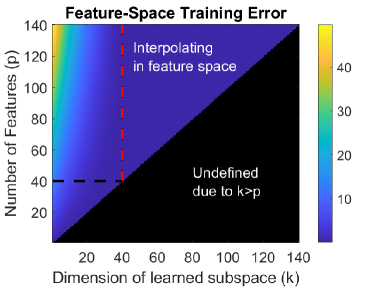
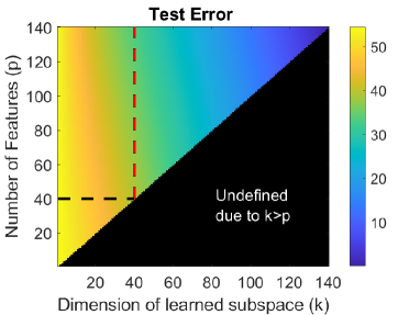
Figure 8: Empirical results for subspace learning based on a class $\mathcal{F}_{p,k}^{\sf DR,orth}(\{\mathbf{u}_{j}\}_{j=1}^{d})$ of linear dimensionality reduction operators as described in Example 5.1. Here, DCT features are employed, $d=140$, $m=20$, $n=40$. Considering the data model in (37), ${\sigma_{\epsilon}=0.5}$ and the true subspace is determined by $\mathbf{B}_{m}$ whose $j^{\sf th}$ column is the properly normalized sum of columns ${\{j+20s\}_{s=0}^{\frac{d}{m}-1}}$ from the ${d\times d}$ DCT matrix. In (a) we present the feature-space training error (i.e., as in the optimization cost in (41)). In (b) we show the test error. Both errors are evaluated as a function of the learned subspace dimension $k$ and the number of features $p$. The $(p,k)$ pairs above the black dashed line correspond to overparameterized settings. The $(p,k)$ pairs to the right of the red dashed line correspond to rank-overparameterized settings.

5.2 The effects of orthonormality constraints and supervision levels on double descent phenomena

Motivated by the lack of double descent phenomena in PCA-based subspace learning, Dar et al. (2020) define a new family of subspace learning problems in order to study their generalization behavior in overparameterized settings. This new family of learning problems connects the PCA-based subspace fitting approach (which is unsupervised and has strict orthonormality constraints on the learned matrix columns) and a regression-based approach (which is fully supervised and does not have orthonormality constraints on the learned matrix). Specifically, Dar et al. (2020) define a supervision-orthonormality plane where each coordinate induces a different subspace learning problem with a unique pair of supervision level and orthonormality constraints on the columns of the learned matrix. The supervision levels range from unsupervised to fully supervised through a gradual range of semi-supervised settings with a varying proportion between the input-only and input-output examples in the training dataset. The orthonormality constraints range from strict to unconstrained through a gradual range of soft orthonormality constraints. The softened orthonormality constraint is implemented by extending the function class (38) into the form of

$$\mathcal{F}_{p,m,\gamma}^{\sf DR,softorth}(\{\mathbf{u}_{j}\}_{j=1}^{d})$$

$$\triangleq\Bigg{\{}f(\mathbf{x})=\mathbf{A}_{m}^{T}\mathbf{U}_{p}^{T}\mathbf{x}~{}\Bigg{|}~{}\mathbf{x}\in\mathbb{R}^{d},\mathbf{A}_{m}\in\mathbb{R}^{p\times m},\rvert\sigma_{j}^{2}\{\mathbf{A}_{m}\}-1\lvert\leq\gamma~{}\text{for }j=1,\dots,m\Bigg{\}},$$ (43)

where $\gamma\geq 0$ determines the softness of the orthonormality constraint, and $\sigma_{j}\{\mathbf{A}_{m}\}$ is the $j^{\sf th}$ singular value of $\mathbf{A}_{m}$. Note that the latent dimension $m$ is known due to the availability of true latent vectors $\mathbf{z}$ in the supervised training data. The orthonormality constraints in Equation (5.2) are defined by the size of the interval around 1 that the singular values of the learned matrix are allowed to reside in. The problem is more orthonormally constrained as the singular values are limited to a smaller interval around 1. Specifically, constraining all singular values to 1 provides a solution with orthonormal columns as in Equation (38).

Using this supervision-orthonormality plane, Dar et al. (2020) show that double descent phenomena become more evident as the subspace learning problem is more supervised and less orthonormally constrained. The majority of the problems on the supervision-orthonormality plane do not have closed-form solutions and, therefore, are empirically evaluated using an optimization framework based on projected gradient descent. These results also emphasize the influence of supervision level on generalization behavior under overparameterization, even beyond the scope of subspace learning.

6 Additional overparameterized learning problems

In this section, we survey recent research on interpolating models in various other modern ML tasks, including data generation, transfer learning, pruning of learned models, and dictionary learning.

6.1 Data generation

Data generation applications aim to produce new instances from a data class that its accurate description is unknown and only a set of its examples are given. Data generation is ubiquitous in deep learning practice, mainly in various architectures that follow the generative adversarial network (GAN) concept (Goodfellow et al., 2014). The idea of a GAN is to jointly train a generator network that produces synthetic instances from the desired class, and a discriminator network that evaluates the generator performance by identifying its synthetic outputs versus true samples from the data class. State-of-the-art practical GANs include highly complex generator and discriminator networks — consequently, understanding overparameterized GANs is a fundamental and important question.

Luzi et al. (2021) provide the first and, to the best of our knowledge, the only explicit study on interpolation phenomena (including double descent) in overparameterized GANs. The study by Luzi et al. (2021) is focused mainly on linear GANs that are overparameterized in the sense that their learned latent dimension is large with respect to the number of examples. This perspective on overparameterized GANs reveals a new behavior of test errors when examined with respect to the learned latent dimension: all interpolating solutions have the same generalization ability, which is often much worse than the best generalization in the non-interpolating (i.e., underparameterized) range of solutions. This theoretical result applies to generative models beyond linear GANs: interpolating solutions generalize equivalently in any generative model that is trained through minimization of a distribution metric or $f$-divergence.

Regardless of interpolation and overparameterization aspects, one can compute the PCA of the given data distribution for training a linear generator with respect to squared error loss, quadratic discriminator and Gaussian data (Feizi et al., 2020). Moreover, extending the unsupervised nature of PCA to include supervised training examples yields double descent phenomena when overparameterization is considered (Dar et al., 2020). Accordingly, Luzi et al. (2021) were motivated to include supervised examples in the training of linear GANs. Truly supervised examples are not realistic due to the need of the true latent representations of the data of interest. Therefore, Luzi et al. (2021) empirically establish the concept of pseudo-supervised training of GANs, which is done by associating the data examples with random latent representations drawn from an isotropic Gaussian distribution. This approach induces test error curves that have double descent and, sometimes, triple descent shapes. More importantly, this pseudo-supervised approach to GAN training was shown to improve generalization performance and to reduce training time, both for linear models with synthetic Gaussian data and for multi-layer nonlinear models with MNIST digit images.

6.2 Transfer learning

Transfer learning is a popular approach for training a DNN to solve a desired target problem, based on another DNN that was already learned for a related source problem. In practice, one or more layers of the source DNN are transferred to the target DNN and set fixed, finely tuned, or used to initialize a full training process. Provided that the source DNN is adequately trained using a large dataset, such transfer learning helps to address the challenges in training a highly overparameterized target DNN using a relatively smaller amount of data, and possibly faster.

A solid base for a fundamental understanding of transfer learning was recently laid by recent analytical results for transfer learning under linear models (Lampinen and Ganguli, 2019; Dar and Baraniuk, 2020; Obst et al., 2021; Dar and Baraniuk, 2021). The first study on double descent phenomena in transfer learning was provided by Dar and Baraniuk (2020) for a setting of two linear regression problems, where a subset of the target parameters is fixed to values transferred from an already computed least squares solution of the related source task. Dar and Baraniuk (2020) analytically characterized a two-dimensional double descent phenomena of the test error of the target task when evaluated with respect to the number of free parameters in the target and source solutions. They defined a noisy linear model to relate the true parameters of the target and source tasks and showed how the generalization error of the target task is affected by the interplay among the structure of the task relation, layout of the true parameters, and the subset of transferred parameters. Their results describe when parameter transfer is useful, and emphasize a fundamental tradeoff between overparameterized learning and transfer learning. In particular, when the source task solution plays a more significant role in the target task solution it also limits the actual overparameterization level. Thus, the best combination of transfer learning and overparameterization depends on the specific problem setting.

The idea that transfer learning counterbalances overparameterization is further emphasized in a second study by Dar and Baraniuk (2021), which utilize the least squares source solution to explicitly regularize the target linear regression problem. Specifically, the target task solution is penalized for its $\ell_{2}$-distance from the source task solution after transformation by the task relation model (which is assumed to be known in this work). This method can be also perceived as implementing a fine tuning procedure. This approach for transfer learning is able to regularize overparameterized learning in a way that mitigates the test error peak that is typically present in double descent phenomena. Moreover, this regularization-based implementation of transfer learning can achieve better generalization than using a regularizer that relies on the true prior of the unknown parameters. This is especially remarkable in the isotropic Gaussian case where using the true prior in a ridge regression approach provides the minimum mean squared error (MMSE) solution of the individual target task, which is still outperformed by transfer learning from a sufficiently related source task.

Another analytical study by Dhifallah and Lu (2021) considers transfer learning between two, possibly nonlinear, single-layer models. They examine general convex loss functions that makes their insights relevant to both regression and classification problems. Their transfer learning formulations include ridge regularization and a regularizer on the distance between the target and source task solutions (the second regularizer can be reduced into the particular case where the transferred parameters are set fixed in the target solution). Recall that Dar and Baraniuk (2020) examined transfer learning from a source task that can interpolate its training data, and therefore emphasize how the double descent phenomenon in the source task affect the generalization performance of the target task. In contrast, the focus in Dhifallah and Lu (2021) is on problems that are more regularized, including ridge regularization in the source task solution that prevents it from interpolating its data. The works by Dar and Baraniuk (2020) and Dhifallah and Lu (2021) both consider Gaussian settings and analytically characterize the conditions on the relation between the target and source tasks that yield beneficial transfer learning.

In a more recent study, Gerace et al. (2021) examine the fundamentals of transfer learning between two-layer networks (including ReLU nonlinearities) for binary classification problems. Specifically, they develop asymptotic characterization of the test errors based on a correlated hidden manifold model, which relies on Gaussian distributions, for the relation between the two tasks (the definition and other utilizations of the hidden manifold model are provided by Goldt et al. (2020); Gerace et al. (2020)). Compared to previous studies (that were focused on single-layer models), the transfer learning in two-layer models allows Gerace et al. (2021) to better emphasize the aspect of feature reuse. Their transfer learning includes regularization on both the source and target tasks and, accordingly, the double descent phenomena are somewhat attenuated — although still noticeable. In their main analytical setting, the first layer in source network is transferred and set fixed in the target network; therefore, this construction can be perceived as the transfer learning counterpart of the well-known random feature model (Rahimi and Recht, 2007), which is also evaluated as an alternative to transfer learning. They also empirically demonstrate (for both synthetic and real data) the beneficial settings for the examined transfer learning when compared to fine tuning and learning the two-layer network from scratch.

6.3 Pruning of learned models

While DNNs are highly parameterized models, it is also common to prune them into less complex forms that better trade off between generalization performance and computational/memory requirements. This is especially useful for applications with limitations on storage space for the learned model, as well as constraints on computation time and energy consumption for processing new inputs.

In general, model pruning is at the expense of higher overparameterization, and therefore the study of their interplay is of great interest. Chang et al. (2021) provided the first theoretical study on pruning of interpolating models and their double descent phenomena. Their main focus is on a pruning approach where a dense model is trained, pruned and then retrained over the support of coordinates that were not pruned. Hence, their pruning is a sparsifying method that defines a support of nonzero values within the entire model. Chang et al. (2021) consider three types of pruning rules: based on magnitude of values, based on the Hessian, and based on oracle knowledge of the best support that minimizes the test error for a desired model sparsity.

Chang et al. (2021) show that overparameterization in the dense model before pruning can lead to improved generalization in the pruned model (i.e., the improvement is with respect to pruned models with the same sparsity level but with varying degrees of parameterization of the dense, pre-pruning model). Moreover, such pruning strategy can induce better generalization than training from scratch a model of the same size (as the pruned model). They also demonstrate double descent phenomena of test errors of the pruned model as a function of the parameterization level of the dense (pre-pruning) model. The concrete setting that they analyze is the minimum $\ell_{2}$-norm solution in overparameterized linear regression on data that satisfies a spiked covariance model. Their theoretical results rely on an asymptotic distributional characterization of the minimum-norm solution of the dense model; specifically, they construct a Gaussian distribution with identical second-order statistics to the original data that may not be Gaussian. Chang et al. (2021) also consider a random feature model in which a first layer (of fixed weights) computes random projections that go into ReLU nonlinearities, followed by a second layer that is learned. They consider pruning of the first layer of (non-learned) random features, which conceptually corresponds to pruning a hidden layer in a network. They show double descent phenomena of the test error as a function of the number of random features. This further emphasizes the finding that overparameterization is beneficial even when pruning is applied.

6.4 Dictionary learning for sparse representations

Dictionary learning is an unsupervised task of establishing an overcomplete dictionary for sparse representation of a given set of data examples. Sulam et al. (2020) consider learned dictionaries that include more atoms (columns in the dictionary matrix) than the true dictionary that generated the training data. They refer to such learned dictionaries as over-realized. Over-realized dictionaries can be learned to achieve zero training error, i.e., to provide perfect sparse representations of the training data. Hence, over-realized dictionaries constitute a particular type of overparameterized model. Sulam et al. (2020) show that over-realized dictionaries can generalize better than those of the ground-truth size in sparse representations of new test data from the same model. Regarding estimation of the true dictionary, they show that learning a dictionary of the true size can be outperformed by first learning an over-realized dictionary and then distilling it into a dictionary of the true size.

The results by Sulam et al. (2020) show that increasing the dictionary size is useful, but only up to a certain point, after which the performance continuously degrades with the increase in model size. Specifically, their results suggest that the best performance can be obtained by the smallest dictionary that interpolates the training data. Due to the underlying non-convex optimization problem in training, such an interpolating solution is achieved by an over-realized dictionary that is larger than the true dictionary.

The learned dictionary can be perceived as a mapping from sparse code vectors to their corresponding data vectors of interest (although the sparse codes are not given in the training data and, thus, the learning is unsupervised). Hence, it is interesting to note that the error curves of learned over-realized dictionary do not exhibit double descent phenomena like in interpolating solutions to linear regression. A likely reason for the lack of double descent in over-realized dictionaries is that their construction via well-established methods (such as K-SVD (Aharon et al., 2006) or the online dictionary learning (Mairal et al., 2010)) is numerically stable and structurally constrained (e.g., dictionary columns are normalized). Thus, despite the ability of the over-realized dictionaries by Sulam et al. (2020) to interpolate their training data, they are not necessarily minimum-norm solutions. An interesting research direction for future work would be to define and study over-realized dictionaries with minimum-norm properties.

7 Open questions

The TOPML research area has received considerable attention in the last few years. While impressive progress has been made, that significantly improves our understanding of overparameterized learning, several important scientific challenges remain to be resolved. In this section we briefly discuss some of the major open questions in the TOPML field.

7.1 Interpolation vs. regularization: Is interpolation simply harmless or actually beneficial?

The setting of overparameterized linear regression allows us to make an explicit mathematical comparison between interpolating and regularized solutions. Consider the $s$-sparse high-dimensional linear model, one of the simplest examples of overparameterized linear regression. In Section 3.3, we mentioned that the best test error among all interpolating solutions will scale as $\Theta\left(\frac{s\log(p/s)}{n}+\frac{n}{p}\right)$. On the other hand, optimally regularized solutions (such as the Lasso) would incur a strictly better MSE of $\Theta\left(\frac{s\log(p/s)}{n}\right)$.  Hastie et al. (2019) also show that optimally regularized ridge regression (where the regularization parameter can be chosen via cross-validation) dominates the minimum $\ell_{2}$-norm interpolation in test performance. As one would expect, they also show that this regularization mitigates the peak in the double descent curve. Indeed, Nakkiran et al. (2020) also demonstrate (in follow-up work to their original work on deep double descent (Nakkiran et al., 2019)) this benefit of regularization, including empirically for DNNs. Furthermore, Mignacco et al. (2020) study how regularization mitigates the double descent peak in a classification task of separating data from a mixture of two Gaussians.

These results suggest that optimally tuned regularization will always dominate interpolation. From this perspective, the recent flurry of results show that interpolation is relatively harmless, rather than being relatively beneficial. However, to obtain the full extent of benefit of regularization over interpolation, we need to optimally tune the regularization parameter. This is usually unknown and needs to be estimated from data. While this can be done via estimating the noise variance, or more generally cross-validation (as formally shown in (Hastie et al., 2019)), such techniques usually require a strong i.i.d. assumption on the noise in the data and will not easily work for less friendly noise models, such as adversarial, correlated, or heteroskedastic noise. In such situations, an overly conservative choice of regularizer might preclude the benefits afforded by interpolation in settings with minimal noise. From a practitioner’s point of view, running iterative algorithms to completion (thus interpolating the data) may be more convenient than formulating a complex early stopping rule that will admit only minimally beneficial performance in practice (Neyshabur et al., 2014). In summary, the decision of whether to interpolate or regularize contains several theoretical and practical nuances and often depends on the context surrounding model deployment. We expect this debate to continue for the foreseeable future.

7.2 Are there applications other than ML where interpolating solutions are useful?

Theoretical research on interpolating solutions mainly attempts to explain the corresponding deep learning practice, which is far ahead of existing theories. Ideally, we can expect that new fundamental insights will induce novel extensions to contemporary practice. Another important question is whether recent theoretical findings on overparameterized interpolating solutions can lead to significant breakthroughs in domains other than ML. As an example consider signal estimation tasks, such as signal deconvolution and inverse problems, that receive degraded measurements of a specific signal without any particular examples of other signals. Another application area to explore is distributed optimization.

In general, the relevance of interpolating solutions in various problems is not a simple wish. As a fundamental example, we note that ML research on interpolating solutions in supervised learning is focused on random design settings where both the inputs and outputs are randomly drawn from an unknown but identical distribution. In particular, the training data is in general different from the test data. Therefore, in this random design setting, interpolating the input-output mappings of the training data does not prevent good performance on new inputs at test time. Supervised learning in random design settings is in accordance with contemporary ML frameworks where, indeed, interpolating solutions can provide remarkable performance. In contrast, classical statistics usually considers a fixed design setting in which the inputs are fixed (possibly set by the experiment designer) and the outputs are random. Specifically, training and test data include the same inputs but matched to different random outputs. Hence, in fixed design settings, a mapping that interpolates the input-output training examples is likely to seriously fail when applied on test inputs.

Let us consider the signal denoising problem to demonstrate the difference between random and fixed designs:

• The denoising problem in the random design can take the following form. The given training dataset includes $n$ examples of noisy signals and their corresponding underlying, noiseless signals. Each of the $n$ examples corresponds to a different signal from the same class. The noiseless and the noisy signals are both $p$-dimensional vectors. In this random design, the goal is to learn a denoising mapping that takes a $p$-dimensional noisy signal and outputs a $p$-dimensional estimate for the corresponding noiseless signal. It is of interest that this mapping will operate well on new noisy signals from the considered class, but that were not included in the training dataset. Following the main principles that we overviewed in this paper, in this case of random-design signal denoising, a learned mapping that interpolates the $n$ training examples does not necessarily imply poor performance on new data.

• The denoising problem in the fixed design can be defined as follows. The given data includes $n$ noisy measurements of the same signal, each measurement is a $p$-dimensional vector of noisy values of the signal over a uniformly-spaced grid of coordinates (i.e., we consider a discrete version of a continuous-domain signal). Examples for noiseless or noisy versions of other signals are not given. In this fixed design, the goal is to estimate the true, noiseless signal values (only) in the $p$ coordinates of the uniformly-spaced grid. The inputs are considered to be the $p$ coordinates of the uniformly-spaced grid. The estimate and the $n$ noisy measurements have the same discrete grid of $p$ coordinates; hence, not only that interpolation is impossible when $n>1$, it would be an incredibly poor estimate when $n=1$.

The above example simply demonstrates why interpolating solutions are irrelevant in many applications and, accordingly, that it is not trivial to find applications other than ML where interpolating solutions are beneficial. Yet, the success of interpolation in modern ML suggests to explore its relevance to other areas.

7.3 How should we define learned model complexity?

The correct definition of learned model complexity is an essential component of TOPML research. Recall that we defined a scenario to be overparameterized when the learned model complexity is high compared to the number of training examples. Thus, the definition of learned model complexity is clearly crucial for understanding whether a specific learning setting is in fact overparameterized. While this basic decision problem (i.e. whether a setting is overparameterized or not) can be solved by identifying whether the learned model interpolates or achieves zero training error, quantifying the actual extent of overparameterization is more challenging as well as more valuable as it allows us to distinguish various interpolating models. The summary of results in Section 3 of this paper showed a diversity of possible generalization behaviors for interpolating models. Whether we can interpret these results through a new overarching notion of learned model complexity remains a largely open question.

In linear models such as in LS regression, model complexity is often measured by the number of learned parameters in the solution. However, the double descent behavior clearly shows that the number of parameters is a misleading measure of learned model complexity; regularization in the learning process, as well as structural redundancies in the architecture may reduce the effective complexity of the learned model. Moreover, the definition of complexity of nonlinear and multi-layer models, including the extreme case of deep neural networks, becomes highly intricate. Model complexity measures that depend on the training data (e.g., Rademacher complexity (Bartlett and Mendelson, 2002)) are useful to understand classical ML via uniform convergence analyses. In contrast, such complexity measures fail to explain the good generalization ability in contemporary settings where the learned models interpolate their training data (Belkin et al., 2018b; Nagarajan and Kolter, 2019; Bartlett and Long, 2020). Researchers have also recently attempted, with relatively more success, to relate other classical notions of learned model complexity to the overparameterized regime. Recently, Dwivedi et al. (2020) adapted Rissanen’s classical notion of minimum description length (MDL) (Rissanen, 1978, 1983) to the overparameterized regime: their data-driven notion of MDL explains some of the behaviors observed in Section 3. Algorithm-dependent notions of model complexity, such as algorithmic stability (Bousquet and Elisseeff, 2002), are also interesting to consider; indeed, Rangamani et al. (2020) recently showed that in some cases, the minimum Hilbert-norm interpolation for kernel regression is also the most algorithmically stable. Much work remains to be done to systematically study these complexity measures in the overparameterized regime and understand whether they are always predictive of generalization behavior. Accordingly, the definition of an appropriate complexity measure continues to pose a fundamental challenge that is at the heart of the TOPML research area.

We thank all the organizers and participants of the inaugural TOPML workshop for extensive discussions and contributions that enriched the content in this survey. Special thanks to Ryan Tibshirani for fruitful discussions on the definition of TOPML and the open questions of the field.

VM thanks her co-authors for several insightful discussions that inspired the treatment of TOPML in this survey; special thanks goes to Anant Sahai for influencing the signal processing-oriented treatment of minimum-norm interpolation provided in Section 3.2 of this paper.

YD and RGB acknowledge support from NSF grants CCF-1911094, IIS-1838177, and IIS-1730574; ONR grants N00014-18-12571, N00014-20-1-2534, and MURI N00014-20-1-2787; AFOSR grant FA9550-18-1-0478; and a Vannevar Bush Faculty Fellowship, ONR grant N00014-18-1-2047.

References

- Advani et al. (2020) M. S. Advani, A. M. Saxe, and H. Sompolinsky. High-dimensional dynamics of generalization error in neural networks. Neural Networks, 132:428–446, 2020.
- Aharon et al. (2006) M. Aharon, M. Elad, and A. Bruckstein. K-SVD: An algorithm for designing overcomplete dictionaries for sparse representation. IEEE Transactions on Signal Processing, 54(11):4311–4322, 2006.
- Akaike (1998) H. Akaike. Information theory and an extension of the maximum likelihood principle. In Selected Papers of Hirotugu Akaike, pages 199–213. Springer, 1998.
- Ardeshir et al. (2021) N. Ardeshir, C. Sanford, and D. Hsu. Support vector machines and linear regression coincide with very high-dimensional features. arXiv preprint arXiv:2105.14084, 2021.
- Aubin et al. (2020) B. Aubin, F. Krzakala, Y. Lu, and L. Zdeborová. Generalization error in high-dimensional perceptrons: Approaching Bayes error with convex optimization. In Advances in Neural Information Processing Systems, volume 33, pages 12199–12210, 2020.
- Banburski et al. (2021) A. Banburski, F. De La Torre, N. Pant, I. Shastri, and T. Poggio. Distribution of classification margins: Are all data equal? arXiv preprint arXiv:2107.10199, 2021.
- Bartlett (1998) P. L. Bartlett. The sample complexity of pattern classification with neural networks: the size of the weights is more important than the size of the network. IEEE Transactions on Information Theory, 44(2):525–536, 1998.
- Bartlett and Long (2020) P. L. Bartlett and P. M. Long. Failures of model-dependent generalization bounds for least-norm interpolation. arXiv preprint arXiv:2010.08479, 2020.
- Bartlett and Mendelson (2002) P. L. Bartlett and S. Mendelson. Rademacher and Gaussian complexities: Risk bounds and structural results. Journal of Machine Learning Research, 3(Nov):463–482, 2002.
- Bartlett et al. (2005) P. L. Bartlett, O. Bousquet, and S. Mendelson. Local Rademacher complexities. The Annals of Statistics, 33(4):1497–1537, 2005.
- Bartlett et al. (2006) P. L. Bartlett, M. I. Jordan, and J. D. McAuliffe. Convexity, classification, and risk bounds. Journal of the American Statistical Association, 101(473):138–156, 2006.
- Bartlett et al. (2017) P. L. Bartlett, D. J. Foster, and M. J. Telgarsky. Spectrally-normalized margin bounds for neural networks. In Advances in Neural Information Processing Systems, pages 6240–6249, 2017.
- Bartlett et al. (2020) P. L. Bartlett, P. M. Long, G. Lugosi, and A. Tsigler. Benign overfitting in linear regression. Proceedings of the National Academy of Sciences, 2020.
- Bartlett et al. (2021) P. L. Bartlett, A. Montanari, and A. Rakhlin. Deep learning: a statistical viewpoint. arXiv preprint arXiv:2103.09177, 2021.
- Belkin (2021) M. Belkin. Fit without fear: remarkable mathematical phenomena of deep learning through the prism of interpolation. arXiv preprint arXiv:2105.14368, 2021.
- Belkin et al. (2018a) M. Belkin, D. Hsu, and P. Mitra. Overfitting or perfect fitting? risk bounds for classification and regression rules that interpolate. In Advances in Neural Information Processing Systems, volume 31, 2018a.
- Belkin et al. (2018b) M. Belkin, S. Ma, and S. Mandal. To understand deep learning we need to understand kernel learning. In International Conference on Machine Learning, pages 541–549. PMLR, 2018b.
- Belkin et al. (2019a) M. Belkin, D. Hsu, S. Ma, and S. Mandal. Reconciling modern machine-learning practice and the classical bias–variance trade-off. Proceedings of the National Academy of Sciences, 116(32):15849–15854, 2019a.
- Belkin et al. (2019b) M. Belkin, A. Rakhlin, and A. B. Tsybakov. Does data interpolation contradict statistical optimality? In The 22nd International Conference on Artificial Intelligence and Statistics, pages 1611–1619. PMLR, 2019b.
- Belkin et al. (2020) M. Belkin, D. Hsu, and J. Xu. Two models of double descent for weak features. SIAM Journal on Mathematics of Data Science, 2(4):1167–1180, 2020.
- Ben-David et al. (2012) S. Ben-David, D. Loker, N. Srebro, and K. Sridharan. Minimizing the misclassification error rate using a surrogate convex loss. In Proceedings of the 29th International Coference on International Conference on Machine Learning, pages 83–90, 2012.
- Bickel et al. (2009) P. J. Bickel, Y. Ritov, and A. B. Tsybakov. Simultaneous analysis of Lasso and Dantzig selector. The Annals of Statistics, 37(4):1705–1732, 2009.
- Boufounos and Baraniuk (2008) P. T. Boufounos and R. G. Baraniuk. 1-bit compressive sensing. In 42nd Annual Conference on Information Sciences and Systems, pages 16–21. IEEE, 2008.
- Bousquet and Elisseeff (2002) O. Bousquet and A. Elisseeff. Stability and generalization. The Journal of Machine Learning Research, 2:499–526, 2002.
- Breiman (1996) L. Breiman. Arcing classifiers. Technical report, Citeseer, 1996.
- Breiman and Freedman (1983) L. Breiman and D. Freedman. How many variables should be entered in a regression equation? Journal of the American Statistical Association, 78(381):131–136, 1983.
- Candès et al. (2006) E. J. Candès, J. Romberg, and T. Tao. Robust uncertainty principles: Exact signal reconstruction from highly incomplete frequency information. IEEE Transactions on Information Theory, 52(2):489–509, 2006.
- Cao et al. (2021) Y. Cao, Q. Gu, and M. Belkin. Risk bounds for over-parameterized maximum margin classification on sub-gaussian mixtures. arXiv preprint arXiv:2104.13628, 2021.
- Chang et al. (2021) X. Chang, Y. Li, S. Oymak, and C. Thrampoulidis. Provable benefits of overparameterization in model compression: From double descent to pruning neural networks. In Proceedings of the AAAI Conference on Artificial Intelligence, volume 35, pages 6974–6983, 2021.
- Chatterji and Long (2021) N. S. Chatterji and P. M. Long. Finite-sample analysis of interpolating linear classifiers in the overparameterized regime. Journal of Machine Learning Research, 22(129):1–30, 2021.
- Chen et al. (2001) S. S. Chen, D. L. Donoho, and M. A. Saunders. Atomic decomposition by basis pursuit. SIAM Review, 43(1):129–159, 2001.
- Chinot et al. (2020) G. Chinot, M. Löffler, and S. van de Geer. On the robustness of minimum-norm interpolators. arXiv preprint arXiv:2012.00807, 2020.
- Chizat et al. (2019) L. Chizat, E. Oyallon, and F. Bach. On lazy training in differentiable programming. Advances in Neural Information Processing Systems, 32:2937–2947, 2019.
- Dar and Baraniuk (2020) Y. Dar and R. G. Baraniuk. Double double descent: On generalization errors in transfer learning between linear regression tasks. arXiv preprint arXiv:2006.07002, 2020.
- Dar and Baraniuk (2021) Y. Dar and R. G. Baraniuk. Transfer learning can outperform the true prior in double descent regularization. arXiv preprint arXiv:2103.05621, 2021.
- Dar et al. (2020) Y. Dar, P. Mayer, L. Luzi, and R. G. Baraniuk. Subspace fitting meets regression: The effects of supervision and orthonormality constraints on double descent of generalization errors. In International Conference on Machine Learning (ICML), 2020.
- D’Ascoli et al. (2020) S. D’Ascoli, M. Refinetti, G. Biroli, and F. Krzakala. Double trouble in double descent: Bias and variance(s) in the lazy regime. In Proceedings of the 37th International Conference on Machine Learning, volume 119 of Proceedings of Machine Learning Research, pages 2280–2290. PMLR, 13–18 Jul 2020.
- Deng et al. (2021) Z. Deng, A. Kammoun, and C. Thrampoulidis. A model of double descent for high-dimensional binary linear classification. Information and Inference: A Journal of the IMA, 2021.
- Derezinski et al. (2020) M. Derezinski, F. T. Liang, and M. W. Mahoney. Exact expressions for double descent and implicit regularization via surrogate random design. Advances in Neural Information Processing Systems, 33, 2020.
- Dhifallah and Lu (2020) O. Dhifallah and Y. M. Lu. A precise performance analysis of learning with random features. arXiv preprint arXiv:2008.11904, 2020.
- Dhifallah and Lu (2021) O. Dhifallah and Y. M. Lu. Phase transitions in transfer learning for high-dimensional perceptrons. Entropy, 23(4):400, 2021.
- Drucker and Cortes (1996) H. Drucker and C. Cortes. Boosting decision trees. Advances in Neural Information Processing Systems, pages 479–485, 1996.
- Dwivedi et al. (2020) R. Dwivedi, C. Singh, B. Yu, and M. J. Wainwright. Revisiting complexity and the bias-variance tradeoff. arXiv preprint arXiv:2006.10189, 2020.
- Dziugaite and Roy (2017) G. K. Dziugaite and D. M. Roy. Computing nonvacuous generalization bounds for deep (stochastic) neural networks with many more parameters than training data. arXiv preprint arXiv:1703.11008, 2017.
- Engl et al. (1996) H. W. Engl, M. Hanke, and A. Neubauer. Regularization of inverse problems, volume 375. Springer Science & Business Media, 1996.
- Feizi et al. (2020) S. Feizi, F. Farnia, T. Ginart, and D. Tse. Understanding GANs in the LQG setting: Formulation, generalization and stability. IEEE Journal on Selected Areas in Information Theory, 2020.
- Foucart (2014) S. Foucart. Stability and robustness of -minimizations with Weibull matrices and redundant dictionaries. Linear Algebra and its Applications, 441:4–21, 2014.
- Friedman et al. (2001) J. Friedman, T. Hastie, and R. Tibshirani. The elements of statistical learning, volume 1. Springer, 2001.
- Friedman (1997) J. H. Friedman. On bias, variance, 0/1—loss, and the curse-of-dimensionality. Data Mining and Knowledge Discovery, 1(1):55–77, 1997.
- Gao and Zhou (2013) W. Gao and Z.-H. Zhou. On the doubt about margin explanation of boosting. Artificial Intelligence, 203:1–18, 2013.
- Geiger et al. (2020) M. Geiger, A. Jacot, S. Spigler, F. Gabriel, L. Sagun, S. d’Ascoli, G. Biroli, C. Hongler, and M. Wyart. Scaling description of generalization with number of parameters in deep learning. Journal of Statistical Mechanics: Theory and Experiment, 2020(2):023401, 2020.
- Geman et al. (1992) S. Geman, E. Bienenstock, and R. Doursat. Neural networks and the bias/variance dilemma. Neural computation, 4(1):1–58, 1992.
- Gerace et al. (2020) F. Gerace, B. Loureiro, F. Krzakala, M. Mézard, and L. Zdeborová. Generalisation error in learning with random features and the hidden manifold model. In International Conference on Machine Learning, pages 3452–3462. PMLR, 2020.
- Gerace et al. (2021) F. Gerace, L. Saglietti, S. S. Mannelli, A. Saxe, and L. Zdeborová. Probing transfer learning with a model of synthetic correlated datasets. arXiv preprint arXiv:2106.05418, 2021.
- Goldt et al. (2020) S. Goldt, M. Mézard, F. Krzakala, and L. Zdeborová. Modeling the influence of data structure on learning in neural networks: The hidden manifold model. Phys. Rev. X, 10:041044, 2020.
- Goodfellow et al. (2014) I. Goodfellow, J. Pouget-Abadie, M. Mirza, B. Xu, D. Warde-Farley, S. Ozair, A. Courville, and Y. Bengio. Generative adversarial nets. Advances in Neural Information Processing Systems, 27, 2014.
- Gordon (1985) Y. Gordon. Some inequalities for Gaussian processes and applications. Israel Journal of Mathematics, 50(4):265–289, 1985.
- Hastie et al. (2019) T. Hastie, A. Montanari, S. Rosset, and R. J. Tibshirani. Surprises in high-dimensional ridgeless least squares interpolation. arXiv preprint arXiv:1903.08560, 2019.
- Hsu et al. (2021) D. Hsu, V. Muthukumar, and J. Xu. On the proliferation of support vectors in high dimensions. In International Conference on Artificial Intelligence and Statistics, pages 91–99. PMLR, 2021.
- Hui and Belkin (2020) L. Hui and M. Belkin. Evaluation of neural architectures trained with square loss vs cross-entropy in classification tasks. arXiv preprint arXiv:2006.07322, 2020.
- Ji and Telgarsky (2019) Z. Ji and M. Telgarsky. The implicit bias of gradient descent on nonseparable data. In Conference on Learning Theory, pages 1772–1798, 2019.
- Jiang et al. (2020) Y. Jiang, P. Foret, S. Yak, D. M. Roy, H. Mobahi, G. K. Dziugaite, S. Bengio, S. Gunasekar, I. Guyon, and B. Neyshabur. NeurIPS 2020 competition: Predicting generalization in deep learning. arXiv preprint arXiv:2012.07976, 2020.
- Johnstone and Lu (2009) I. M. Johnstone and A. Y. Lu. On consistency and sparsity for principal components analysis in high dimensions. Journal of the American Statistical Association, 104(486):682–693, 2009.
- Kammoun and Alouini (2021) A. Kammoun and M.-S. Alouini. On the precise error analysis of support vector machines. IEEE Open Journal of Signal Processing, 2:99–118, 2021.
- Kobak et al. (2020) D. Kobak, J. Lomond, and B. Sanchez. The optimal ridge penalty for real-world high-dimensional data can be zero or negative due to the implicit ridge regularization. Journal of Machine Learning Research, 21:169–1, 2020.
- Koehler et al. (2021) F. Koehler, L. Zhou, D. J. Sutherland, and N. Srebro. Uniform convergence of interpolators: Gaussian width, norm bounds, and benign overfitting. arXiv preprint arXiv:2106.09276, 2021.
- Krahmer et al. (2018) F. Krahmer, C. Kümmerle, and H. Rauhut. A quotient property for matrices with heavy-tailed entries and its application to noise-blind compressed sensing. arXiv preprint arXiv:1806.04261, 2018.
- Lampinen and Ganguli (2019) A. K. Lampinen and S. Ganguli. An analytic theory of generalization dynamics and transfer learning in deep linear networks. In International Conference on Learning Representations (ICLR), 2019.
- Liang and Rakhlin (2020) T. Liang and A. Rakhlin. Just interpolate: Kernel “ridgeless” regression can generalize. The Annals of Statistics, 48(3):1329–1347, 2020.
- Liang and Recht (2021) T. Liang and B. Recht. Interpolating classifiers make few mistakes. arXiv preprint arXiv:2101.11815, 2021.
- Liang and Sur (2020) T. Liang and P. Sur. A precise high-dimensional asymptotic theory for boosting and min-l1-norm interpolated classifiers. arXiv preprint arXiv:2002.01586, 2020.
- Liao et al. (2020) Z. Liao, R. Couillet, and M. Mahoney. A random matrix analysis of random fourier features: beyond the gaussian kernel, a precise phase transition, and the corresponding double descent. In 34th Conference on Neural Information Processing Systems (NeurIPS 2020), 2020.
- Lolas (2020) P. Lolas. Regularization in high-dimensional regression and classification via random matrix theory. arXiv preprint arXiv:2003.13723, 2020.
- Luzi et al. (2021) L. Luzi, Y. Dar, and R. G. Baraniuk. Double descent and other interpolation phenomena in GANs. arXiv preprint arXiv:2106.04003, 2021.
- Mai et al. (2019) X. Mai, Z. Liao, and R. Couillet. A large scale analysis of logistic regression: Asymptotic performance and new insights. In IEEE International Conference on Acoustics, Speech and Signal Processing (ICASSP), pages 3357–3361, 2019. 10.1109/ICASSP.2019.8683376.
- Mairal et al. (2010) J. Mairal, F. Bach, J. Ponce, and G. Sapiro. Online learning for matrix factorization and sparse coding. Journal of Machine Learning Research, 11(1), 2010.
- Mei and Montanari (2019) S. Mei and A. Montanari. The generalization error of random features regression: Precise asymptotics and the double descent curve. Communications on Pure and Applied Mathematics, 2019.
- Mei et al. (2021) S. Mei, T. Misiakiewicz, and A. Montanari. Generalization error of random features and kernel methods: hypercontractivity and kernel matrix concentration. arXiv preprint arXiv:2101.10588, 2021.
- Mignacco et al. (2020) F. Mignacco, F. Krzakala, Y. Lu, P. Urbani, and L. Zdeborová. The role of regularization in classification of high-dimensional noisy Gaussian mixture. In International Conference on Machine Learning, pages 6874–6883. PMLR, 2020.
- Mitra (2019) P. P. Mitra. Understanding overfitting peaks in generalization error: Analytical risk curves for and penalized interpolation. arXiv preprint arXiv:1906.03667, 2019.
- Montanari et al. (2019) A. Montanari, F. Ruan, Y. Sohn, and J. Yan. The generalization error of max-margin linear classifiers: High-dimensional asymptotics in the overparametrized regime. arXiv preprint arXiv:1911.01544, 2019.
- Muthukumar et al. (2020a) V. Muthukumar, A. Narang, V. Subramanian, M. Belkin, D. Hsu, and A. Sahai. Classification vs regression in overparameterized regimes: Does the loss function matter? arXiv preprint arXiv:2005.08054, 2020a.
- Muthukumar et al. (2020b) V. Muthukumar, K. Vodrahalli, V. Subramanian, and A. Sahai. Harmless interpolation of noisy data in regression. IEEE Journal on Selected Areas in Information Theory, 2020b.
- Nagarajan and Kolter (2019) V. Nagarajan and J. Z. Kolter. Uniform convergence may be unable to explain generalization in deep learning. In Advances in Neural Information Processing Systems, pages 11611–11622, 2019.
- Nakkiran et al. (2019) P. Nakkiran, G. Kaplun, Y. Bansal, T. Yang, B. Barak, and I. Sutskever. Deep double descent: Where bigger models and more data hurt. arXiv preprint arXiv:1912.02292, 2019.
- Nakkiran et al. (2020) P. Nakkiran, P. Venkat, S. Kakade, and T. Ma. Optimal regularization can mitigate double descent. arXiv preprint arXiv:2003.01897, 2020.
- Neyshabur et al. (2014) B. Neyshabur, R. Tomioka, and N. Srebro. In search of the real inductive bias: On the role of implicit regularization in deep learning. arXiv preprint arXiv:1412.6614, 2014.
- Obst et al. (2021) D. Obst, B. Ghattas, J. Cugliari, G. Oppenheim, S. Claudel, and Y. Goude. Transfer learning for linear regression: a statistical test of gain. arXiv preprint arXiv:2102.09504, 2021.
- Pati et al. (1993) Y. C. Pati, R. Rezaiifar, and P. S. Krishnaprasad. Orthogonal matching pursuit: Recursive function approximation with applications to wavelet decomposition. In Conference Record of The Twenty-Seventh Asilomar Conference on Signals, Systems and Computers, pages 40–44. IEEE, 1993.
- Paul (2007) D. Paul. Asymptotics of sample eigenstructure for a large dimensional spiked covariance model. Statistica Sinica, pages 1617–1642, 2007.
- Rahimi and Recht (2007) A. Rahimi and B. Recht. Random features for large-scale kernel machines. In Proceedings of the 20th International Conference on Neural Information Processing Systems, page 1177–1184, 2007.
- Rangamani et al. (2020) A. Rangamani, L. Rosasco, and T. Poggio. For interpolating kernel machines, minimizing the norm of the ERM solution minimizes stability. arXiv preprint arXiv:2006.15522, 2020.
- Rao (1971) P. Rao. Some notes on misspecification in multiple regressions. The American Statistician, 25(5):37–39, 1971.
- Rissanen (1978) J. Rissanen. Modeling by shortest data description. Automatica, 14(5):465–471, 1978.
- Rissanen (1983) J. Rissanen. A universal prior for integers and estimation by minimum description length. The Annals of statistics, 11(2):416–431, 1983.
- Rosset et al. (2004) S. Rosset, J. Zhu, and T. Hastie. Boosting as a regularized path to a maximum margin classifier. The Journal of Machine Learning Research, 5:941–973, 2004.
- Salehi et al. (2019) F. Salehi, E. Abbasi, and B. Hassibi. The impact of regularization on high-dimensional logistic regression. In Advances in Neural Information Processing Systems, volume 32, 2019.
- Salehi et al. (2020) F. Salehi, E. Abbasi, and B. Hassibi. The performance analysis of generalized margin maximizers on separable data. In International Conference on Machine Learning, pages 8417–8426. PMLR, 2020.
- Saligrama and Zhao (2011) V. Saligrama and M. Zhao. Thresholded basis pursuit: LP algorithm for order-wise optimal support recovery for sparse and approximately sparse signals from noisy random measurements. IEEE Transactions on Information Theory, 57(3):1567–1586, 2011.
- Schapire et al. (1998) R. E. Schapire, Y. Freund, P. Bartlett, and W. S. Lee. Boosting the margin: A new explanation for the effectiveness of voting methods. The annals of statistics, 26(5):1651–1686, 1998.
- Schölkopf et al. (2002) B. Schölkopf, A. J. Smola, and F. Bach. Learning with kernels: support vector machines, regularization, optimization, and beyond. MIT Press, 2002.
- Shen et al. (2016) D. Shen, H. Shen, and J. Marron. A general framework for consistency of principal component analysis. The Journal of Machine Learning Research, 17(1):5218–5251, 2016.
- Soudry et al. (2018) D. Soudry, E. Hoffer, M. Shpigel Nacson, S. Gunasekar, and N. Srebro. The implicit bias of gradient descent on separable data. The Journal of Machine Learning Research, 19(1):2822–2878, 2018.
- Spigler et al. (2019) S. Spigler, M. Geiger, S. d’Ascoli, L. Sagun, G. Biroli, and M. Wyart. A jamming transition from under-to over-parametrization affects generalization in deep learning. Journal of Physics A: Mathematical and Theoretical, 52(47):474001, 2019.
- Sulam et al. (2020) J. Sulam, C. You, and Z. Zhu. Recovery and generalization in over-realized dictionary learning. arXiv preprint arXiv:2006.06179, 2020.
- Sur and Candès (2019) P. Sur and E. J. Candès. A modern maximum-likelihood theory for high-dimensional logistic regression. Proceedings of the National Academy of Sciences, 116(29):14516–14525, 2019.
- Taheri et al. (2020) H. Taheri, R. Pedarsani, and C. Thrampoulidis. Sharp asymptotics and optimal performance for inference in binary models. In Proceedings of the Twenty Third International Conference on Artificial Intelligence and Statistics, volume 108, pages 3739–3749. PMLR, 26–28 Aug 2020.
- Taheri et al. (2021) H. Taheri, R. Pedarsani, and C. Thrampoulidis. Fundamental limits of ridge-regularized empirical risk minimization in high dimensions. In Proceedings of The 24th International Conference on Artificial Intelligence and Statistics, volume 130, pages 2773–2781. PMLR, 13–15 Apr 2021.
- Theisen et al. (2021) R. Theisen, J. Klusowski, and M. Mahoney. Good classifiers are abundant in the interpolating regime. In International Conference on Artificial Intelligence and Statistics, pages 3376–3384. PMLR, 2021.
- Thrampoulidis et al. (2015) C. Thrampoulidis, S. Oymak, and B. Hassibi. Regularized linear regression: A precise analysis of the estimation error. In Conference on Learning Theory, pages 1683–1709. PMLR, 2015.
- Tsigler and Bartlett (2020) A. Tsigler and P. L. Bartlett. Benign overfitting in ridge regression. arXiv preprint arXiv:2009.14286, 2020.
- Vapnik (2013) V. Vapnik. The nature of statistical learning theory. Springer science & business media, 2013.
- Wang and Thrampoulidis (2021) K. Wang and C. Thrampoulidis. Benign overfitting in binary classification of Gaussian mixtures. In IEEE International Conference on Acoustics, Speech and Signal Processing (ICASSP), pages 4030–4034, 2021.
- Wang et al. (2021) K. Wang, V. Muthukumar, and C. Thrampoulidis. Benign overfitting in multiclass classification: All roads lead to interpolation. arXiv preprint arXiv:2106.10865, 2021.
- Wojtaszczyk (2010) P. Wojtaszczyk. Stability and instance optimality for gaussian measurements in compressed sensing. Foundations of Computational Mathematics, 10(1):1–13, 2010.
- Woodworth et al. (2020) B. Woodworth, S. Gunasekar, J. D. Lee, E. Moroshko, P. Savarese, I. Golan, D. Soudry, and N. Srebro. Kernel and rich regimes in overparametrized models. In Conference on Learning Theory, pages 3635–3673. PMLR, 2020.
- Wyner et al. (2017) A. J. Wyner, M. Olson, J. Bleich, and D. Mease. Explaining the success of adaboost and random forests as interpolating classifiers. The Journal of Machine Learning Research, 18(1):1558–1590, 2017.
- Xu and Hsu (2019) J. Xu and D. J. Hsu. On the number of variables to use in principal component regression. In Advances in Neural Information Processing Systems (NeurIPS), pages 5095–5104, 2019.
- Yang et al. (2020) Z. Yang, Y. Yu, C. You, J. Steinhardt, and Y. Ma. Rethinking bias-variance trade-off for generalization of neural networks. In International Conference on Machine Learning, pages 10767–10777. PMLR, 2020.
- Zhang et al. (2017) C. Zhang, S. Bengio, M. Hardt, B. Recht, and O. Vinyals. Understanding deep learning requires rethinking generalization. In ICLR, 2017.
- Zhang et al. (2021) C. Zhang, S. Bengio, M. Hardt, B. Recht, and O. Vinyals. Understanding deep learning (still) requires rethinking generalization. Communications of the ACM, 64(3):107–115, 2021.
- Zhang (2004) T. Zhang. Statistical behavior and consistency of classification methods based on convex risk minimization. Annals of Statistics, pages 56–85, 2004.
- Zhou et al. (2020) L. Zhou, D. J. Sutherland, and N. S. On uniform convergence and low-norm interpolation learning. arXiv preprint arXiv:2006.05942, 2020.
- Zhuo et al. (2021) J. Zhuo, J. Kwon, N. Ho, and C. Caramanis. On the computational and statistical complexity of over-parameterized matrix sensing. arXiv preprint arXiv:2102.02756, 2021.