Tensor Normalization and Full Distribution Training

Abstract

In this work, we introduce pixel wise tensor normalization, which is inserted after rectifier linear units and, together with batch normalization, provides a significant improvement in the accuracy of modern deep neural networks. In addition, this work deals with the robustness of networks. We show that the factorized superposition of images from the training set and the reformulation of the multi class problem into a multi-label problem yields significantly more robust networks. The reformulation and the adjustment of the multi class log loss also improves the results compared to the overlay with only one class as label. https://atreus.informatik.uni-tuebingen.de/seafile/d/8e2ab8c3fdd444e1a135/?p=%2FTNandFDT&mode=list

1 Introduction

Deep neural networks are the state of the art in many areas of image processing. The application fields are image classification [23, 25, 47, 48, 33, 8, 9, 18, 20, 21], semantic segmentation [15, 27, 11], landmark regression [45, 19, 49], object detection [51, 17, 34, 24, 16, 14, 12, 36], and many more. In the real world, this concerns autonomous driving, human-machine interaction [38, 10, 35], eye tracking [7, 30, 29, 31, 26, 32, 53, 52, 13, 50], robot control, facial recognition, medical diagnostic systems, and many other areas [39, 28, 46]. In all these areas, the accuracy, reliability, and provability of the networks is very important and thus a focus of current research in machine learning [22, 40, 42, 43, 41, 37]. The improvement of accuracy is achieved, on the one hand, by new layers that improve internal processes through normalizations [68, 94, 66, 91, 106, 100, 67] or focusing on specific areas either on the input image or in the internal tensors [102, 65, 64]. Another optimization focus are the architectures of the models, through this considerable success has been achieved in recent years via ResidualNets [62], MobileNets [95], WideResnets  [110], PyramidNets [60], VisonTransformers [6], and many more. In the area of robustness and reliability of neural networks, there has been considerable progress in the area of attack possibilities on the models [57, 81, 2, 74] as well as in their defense [87, 98, 86, 63, 99, 97].

1.1 Contribution of this work:

• A novel pixel wise tensor normalization layer which does not require any parameter and boosts the performance of deep neuronal networks.

• The factorized superposition of training images, which boosts the robustness of deep neural networks.

• Using a multi label loss softmax formulation to boost the accuracy of the robust models trained with the factorized superposition of training images.

1.2 Normalization in DNNs

Normalization of the output is the most common use of internal manipulation in DNNs today. The most famous representative is the batch normalization(BN) [68]. This approach subtracts the mean and divides the output with the standard deviation, both are computed over several batches. In addition, the output is scaled and shifted by an offset. Those two values are also computed over several batches. Another type of output normalization is the group normalization GN [106]. In this approach, groups are formed to compute the mean and standard deviation, which are used to normalize the group. The advantage of GN in comparison to BN is that it does not require large batches. Other types of output normalization are instance normalization IN [100, 67] and layer normalization LN [1]. LN uses the layers to compute the mean and the standard deviation, and IN uses only each instance individually. IN and LN are used in recurrent neural networks (RNN) [96] or vision transformers [6]. The proposed tensor normalization belongs to this group, since we normalize the output of the rectifier linear units.

Another group of normalization modifies the weights of the model. As for the output normalization, there are several approaches in this domain. The first is the weight normalization (WN) [94, 66]. In WN the weights of a network are multiplied by a constant and divided by the Euclidean distance of the weight vector of a neuron. WN is extended by weight standardization (WS) [91]. WS does not use a constant, but instead computes the mean and the standard deviation of the weights. The normalization is computed by subtracting the mean and dividing by the standard deviation. Another extension to WN is the weight centralization (WC) [44] which computes a two dimensional mean matrix and subtracts it from the weight tensor. This improves the stability during training and improves the results of the final model. The normalization of the weights have the advantage, that they do not have to be applied after the training of the network.

The last group of normalization only affects the gradients of the models. The two most famous approaches are the usage of the first [90] and second momentum [71]. Those two approaches are standard in modern neural network training, since they stabilize the gradients with the updated momentum and lead to a faster training process. The main impact of the first momentum is that it prevents exploding gradients. For the second momentum, the main impact is a faster generalization. These moments are moving averages which are updated in each weight update step. Another approach from this domain is the gradient clipping [88, 89]. In gradient clipping, random gradients are set to zero or modified by a small number. Other approaches map the gradients to subspaces like the Riemannian manifold [59, 79, 5]. The computed mapping is afterwards used to update the gradients. The last approach from the gradient normalization is the gradient centralization (GC) [108] which computes a mean over the current gradient tensor and subtracts it.

1.3 Multi label image classification (MLIC)

In multi label image classification the task is to classify multiple labels correctly based on a given image. Since this is an old computer vision problem various approaches have been proposed here. The most common approach is ranking the labels based on the output distribution. This pairwise ranking loss was first used in [101] and extended by weights to the weighted approximate ranking (WARP) [56, 105]. WARP was further extended by the multi label positive and unlabeled method [70]. This approach mainly focuses on the positive labels which have a high probability to be correct. This of course has the disadvantage that noisy labels have a high negative impact on the approach. To overcome this issue the top-k loss [76, 77, 78] was developed. For the top-k loss there are two representatives namely smooth top-k hinge loss and top-k softmax loss.

Another approach treats the multi label image classification problem as an object detection problem. The follow the two-step approach of the R-CNN object detection method [55] which first detects possible good candidate areas and afterwards classifies them. The first approach in multi label image classification following this object detection approach is [104]. A refinement of this approach is proposed in [111, 84] which uses an RNN on the candidate regions to predict label dependencies. The general disadvantage of the object detection based approach is the requirement of bounding box annotations. Similar to [111, 84] the authors in [103, 69] use a CNN for region proposal but instead of using only the candidate region, the authors use the entire output of the CNN in the RNN to model the label dependencies. Another approach which exploits semantic and spatial relations between labels only using image-level supervision is proposed in [114]. Another approach following the object detection problem concept uses a dual-stream neural network [109]. The advantage is that the model can utilize local features and global image pairs. This approach was further extended by [112] to also detect novel classes.

In the context of large scale image retrieval [113, 75] and dimensionality reduction [82] the multi label classification problem also has an important share to the success. In [113, 75] deep neural networks are proposed to compute feature representations and compact hash codes. While these methods work effectively on multi class datasets like CIFAR 10 [72] they are significantly outperformed on challenging multi-label datasets [58]. [3, 4] proposed a hashing method which is robust to noisy labels and capable of handling the multi label problem. In [73] a dimensionality reduction method was proposed which embeds the features and labels onto a low-dimensional space vector. [82] proposed a semi-supervised dimension reduction method which can handle noisy labels and multi-labeled images.

1.4 Adversarial Robustness

The most common defense strategies against adversarial attacks are adversarial training, defensive distillation and input gradient regularization. Adversarial training uses adversarial attacks during the training procedure or modify the loss function to compensate for input perturbations [57, 81]. The defensive distillation [87] trains models on output probabilities and not on hard labels, as it is done in common multi class image classification.

Another strategy to train robust models is the use of ensembles of models [98, 86, 63, 99, 97]. In [98] for example, 10 models are trained and used in an ensemble. While those ensembles are very robust, they have a high compute and memory consumption, which limits them to smaller models. To overcome the issue of high compute and memory consumption, the idea of ensembles of low-precision and quantized models has been proposed [54]. Those low-precision and quantized models alone have shown a higher adversarial robustness than their full-precision counterparts [54, 85]. The disadvantage of the low-precision and quantized models is the lower accuracy, which is increased by forming ensembles [97]. An alternative approach is presented in [92], where stochastic quantization is used to compute low-precision models out of full-precision models with a higher accuracy and a high adversarial robustness.

2 Method

In this paper, we present two optimizations for deep neural networks. One is the 2D tensor normalization and the other is the training of the full classification distribution and adaptation of the loss function. For this reason, we have divided the method part into two subgroups, in which both methods are described separately.

2.1 Tensor Normalization

The idea behind the tensor normalization is to compensate the shifted value distribution after a rectifier linear unit. Since convolutions are computed locally, it is necessary that this normalization is computed for each $(x,y)$ coordinate separately. This results in a 2D matrix of mean values, which is subtracted from the tensor along the $z$ dimension.

$$TNMean_{x,y}(A)=\frac{\sum_{z=1}^{Z}A_{x,y,z}}{Z}$$ (1)

Equation 1 describes the mean computation for the tensor normalization after the activation function. The tensor $A$ with the size $X,Y,Z$ is used online to compute the current 2D mean matrix $TNMean_{x,y}$ with the dimension $X,Y,1$. Afterwards, this mean is subtracted from each $z$ position of the tensor and therefore, the entire tensor has a zero mean and a less skewed value distribution.

Data: Activation tensor $A$

Result: Normalized activation tensor $A^{*}$

$M=TNMean(A)$

for $i=1;\ i<Z;\ i=i+1$ do

       $A_{i}^{*}=A_{i}-M$

end for

Algorithm 1 Algorithmic workflow of the tensor normalization in the forward pass. For the backward pass, the error values are simply passed backwards, since the subtraction equation in the derivative becomes 1.

Algorithm 1 describes the computation of the tensor normalization in a neural network forward pass. As can be seen it is a simple online computation of the 2D mean matrix of the activation tensor and a subtraction along the depth of the tensor. For the backward pass the error values have just to be passed to the previous layer since the subtraction equation is one in the derivative. Due to this properties, it can be directly computed in the rectifier linear unit. This means it does not require any additional GPU memory.

Our formal justification of "Why Tensor Normalization Improves Generalization of Neural Networks" is based on numerics and properties of large numbers. Mathematically, a neuron is a linear combination $P=D*W+B$ with $P=$Output, $D=$Input data, $W=$Model weights, and $B=$Bias term. If we now normalize our input data $A^{*}=(A-M)$ we get the formula $P=D^{*}*W+B$ with $M=MeanofD$. If we now simply define $B^{*}=B+M*W$, it follows that the normalization should have no effect on the neuron, since it can learn the same function even without the normalization. However, this changes when we consider the numerics and the computation of the derivatives in a neural network.
Suppose we have a one-dimensional input $D$ which is larger or equal than the normalized input $D^{*}=D-M$. The derivative for the weights is given by $\frac{\delta L}{\delta W}=\frac{\delta L}{\delta P}*\frac{\delta P}{\delta W}=(P-GT)*D$ with $L=$Squared loss error function and $GT=$Ground truth. As can be seen the data $D$ is included into the gradient computation of the weights which leads to larger steps in the error hyperplane. In addition, a large $D$ also results in smaller weights $W$ since $W=(P-B)*D^{-1}$. This means a large $D$ produces large gradient updates and searches for a smaller global optima $W$. With a smaller $D^{*}=D-M$ we look for a larger optima $W$ and use smaller gradient updates for this. In addition, the numerical stability of $W$ is higher since computers can only represent a certain accuracy for real numbers.
Proof that $|D^{*}|\leq|D|$: Since we apply the tensor normalization only after rectifier linear units $D\in\mathbb{R}^{+}_{0}$ and therefore $|D|\geq 0$, $|M|\geq 0$, and $|D^{*}|\geq 0$. Now we have to consider three cases $|D|=0,|M|=0$, $|D|>0,|M|=0$, and $|D|>0,|M|>0$. For the first case $|D|=0,|M|=0$, $|D^{*}|$ would also be zero and therefore $|D^{*}|\leq|D|$ holds. The second case $|D|>0,|M|=0$ leads to $D^{*}=D-M=D-0=D$ for which $|D^{*}|\leq|D|$ also holds. In the last case $|D|>0,|M|>0$ we can simply shift $M$ to the other side $D^{*}+M=D$ which shows that $|D^{*}|\leq|D|$ holds again.

2.2 Full Distribution Training

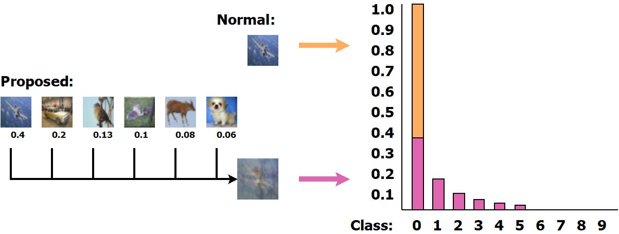
Figure 1: Exemplary illustration of the proposed full distribution training. In orange, the normal approach with one image to one class is shown. In pink, the combination of multiple images to one and the ground truth adaption is shown.

The idea behind the full distribution training is to not restrict the input to correspond to one class only. We combine multiple images using a weighting scheme and use this weighting as corresponding class labels. An example can be seen in Figure 1. For the computation of the weighting scheme, we use the harmonic series and select the amount of combined images randomly up to the amount of different classes. This makes it easier to reproduce our results and since the harmonic series is connected to the coupon collector’s problem or picture collector’s problem we thought it would be a superb fit. The purpose of the full distribution training is a cheap way to train robust models without any additional training time or specialized augmentation and maintaining the accuracy of the model.

$$F_{i}=\frac{\frac{1}{i}}{\sum_{j=1}^{max(C,RND)}F_{j}}$$ (2)

Equation 2 is the harmonic series ($\frac{1}{i}$) normalized by the sum ($\sum_{j=1}^{max(C,RND)}F_{j}$). We had to normalize the series because the harmonic series is divergent even though the harmonic series is a zero sequence. In Equation 2 $C$ represents the amount of classes of the used dataset and $RND$ a randomly chosen number.

$$D=\sum_{i=1}^{max(C,RND)}I_{j=RND}*F_{i}~{}|~{}C(j)\notin C(D)$$ (3)

With the factors from Equation 2 we can compute the new input images using Equation 3. Therefore, we multiply a randomly selected image $I_{j=RND}$ with the corresponding factor $F_{i}$ and combine all images by summing them up. However, there is a special restriction that only one example is allowed for each class ($C(j)\notin C(D)$). This means, that each class in $C(D)$ can only have one or no representative.

$$GT=\sum_{i=1}^{max(C,RND)}L_{j=RND}*F_{i}~{}|~{}C(j)\notin C(GT)$$ (4)

For the computation of the ground truth distribution $GT$ in Equation 4 we follow the same concept as for the images in Equation 3. We select the label $L_{j=RND}$ corresponding to the randomly selected image $I_{j=RND}$ and multiply it by the factor $F_{i}$. The combination is again done by summing all factorized labels together. As for the images, we allow only one example per class or none if the amount of combined images is less than the amount of classes.

Data: Labels $L$, Images $I$, Classes $C$

Result: Ground Truth $GT$, Data $D$

$F=0$;

$GT=0$;

$D=0$;

$Sum=0$

$Amount=max(C,RND)$

for $i=1;\ i<Amount;\ i=i+1$ do

       $F_{i}=1/i$

       $Sum=Sum+F_{i}$

end for

$F=F/Sum$

for $i=1;\ i<Amount;\ i=i+1$ do

       $j=RND(L)~{}|~{}C(j)\notin C(GT)$

       $GT=GT+L_{j}*F_{i}$

       $D=D+I_{j}*F_{i}$

      

end for

Algorithm 2 The creation of a multi label example based on Equations 2, 3, and 4. In the first for loop the factors are computed and normalized. The second loop selects unique class examples and combines them based on the factors.

The algorithmic description of the combination and weighting can be seen in Algorithm 2. In the first for loop we compute the factors, and in the second for loop we combine the images and the labels.

$$Softmax_{i}(P)=\frac{e^{P_{i}}}{\sum_{y=1}^{Y}e^{P_{y}}}$$ (5)

For the multi class classification, the softmax function has prevailed. The softmax function can be seen in Equation 5 and is used to compute an exponentially weighted distribution out of the predicted values. This distribution decouples the numeric values from the loss function so that only the relative value among the values is important, which stabilizes training and leads to a better generalization.

Data: Ground truth $GT$, predictions $P$, Batch size $B$

Result: Error $E$, Loss $L$

$P_{S}=Softmax(P)$;

$Scale=\frac{1}{B}$;

$L=0$

for $b_{i}=1;\ b_{i}<B;\ b_{i}=b_{i}+1$ do

       for $y_{i}=1;\ y_{i}<Y;\ y_{i}=y_{i}+1$ do

             if if $y_{i}==GT(1,b_{i})$ then

                   $L=L+Scale*-log(P_{S}(y_{i},b_{i}))$

                   $P_{S}(y_{i},b_{i})=Scale*(P_{S}(y_{i},b_{i})-1)$

             else

                   $P_{S}(y_{i},b_{i})=Scale*(P_{S}(y_{i},b_{i}))$

             end if

            

       end for

      

end for

Algorithm 3 The calculation of the softmax multi class log function, or also known as entropy loss. It first converts the predictions into a probability distribution using the softmax function. Afterwards, the desired class per batch gets the error based on its distance to 1 (if branch). All other values should be zero, which is why they receive their probability as error (else branch).

For the computation of the loss value and the back propagated error, Algorithm 3 is used in normal multi class classification. As can be seen in the first if statement, this is not sufficient for a multi label problem since we have multiple target values and those are not one ($P_{S}(y_{i},b_{i})=Scale*(P_{S}(y_{i},b_{i})-1)$).

Data: Ground truth $GT$, predictions $P$, Batch size $B$

Result: Error $E$, Loss $L$

$P_{S}=Softmax(P)$;

$Scale=\frac{1}{B}$;

$L=0$

for $b_{i}=1;\ b_{i}<B;\ b_{i}=b_{i}+1$ do

       for $y_{i}=1;\ y_{i}<Y;\ y_{i}=y_{i}+1$ do

             if if $GT(y_{i},b_{i})>\epsilon$ then

                   $L=L+Scale*-log(P_{S}(y_{i},b_{i}))$

                   $P_{S}(y_{i},b_{i})=Scale*(P_{S}(y_{i},b_{i})-GT(y_{i},b_{i}))$

             else

                   $P_{S}(y_{i},b_{i})=Scale*(P_{S}(y_{i},b_{i}))$

             end if

            

       end for

      

end for

Algorithm 4 The calculation of the softmax multi label log function, which we use for the full distribution training. It first converts the predictions into a probability distribution using the softmax function, as it is done in the softmax multi class log function. Afterwards, we use the ground truth distribution to select all classes in the current image ($GT(y_{i},b_{i})>\epsilon$) where $\epsilon$ is a small number greater zero. Based on the ground truth distribution value, we compute the error $(P_{S}(y_{i},b_{i})-GT(y_{i},b_{i}))$. For all other values, we use the same procedure as in the softmax multi class log function (else branch).

Therefore, we modified Algorithm 3 to Algorithm 4 which allows multiple labels with different values. This can be seen in the if condition ($GT(y_{i},b_{i})>\epsilon$) which handles all values greater $\epsilon$ and in the if branch ($P_{S}(y_{i},b_{i})=Scale*(P_{S}(y_{i},b_{i})-GT(y_{i},b_{i}))$) which uses the ground truth value for gradient computation.

Our formal justification that the full distribution training generates more robust networks: A common strategy to train more robust networks is the usage of Projected Gradient Descent (PGD), which for the sake of completeness is described in Section "Projected Gradient Descent (PGD)", during training. PGD computes the gradient of the current image and uses the sign of the gradient $sign(\delta f(x^{t})$ to compute a new modified image $x^{t+1}$. This is done using an iterative scheme and an modification factor $\alpha$. The general equation for PGD is $x^{t+1}=x^{t}+\alpha*\delta f(x^{t})$ whereby the $sign()$ function in Equation 6 is used to avoid that very small gradient values block the attack and feign robustness and also called $l_{\infty}$ norm. Our approach in contrast uses another image $I==x^{0}$ (or multiple images) from another class to modify the current image collection $D==x^{t+1}$. This means, that the gradient to shift one image into the direction of another class is gifted by the dataset itself through an image of another class. The modification equation for our approach is $\sum_{i=1}^{max(C,RND)}I_{j=RND}*F_{i}~{}|~{}C(j)\notin C(D)$ based on Equation 3. If we set $max(C,RND)==2$ we can remove the sum and get $I_{j1}*F_{1}+I_{j2}*F_{2}~{}|~{}C(j1)\neq C(j2)$. Now setting $F_{1}==1$ and $F_{2}==\alpha$ we get $I_{j1}+\alpha*I_{j2}~{}|~{}C(j1)\neq C(j2)$. Since the class of $j1$ is different to the class of $j2$ we can interpret $I_{j2}$ as the gradient to another class and therefore write $I_{j2}=\delta f(I_{j1})$. With this gradient formulation we get $I_{j1}+\alpha*\delta f(I_{j1})$ which is the same as the PGD formulation. This means, that we can get our gradients to another class directly from the dataset and do not have to perform multiple iterations of forward and backward propagation to compute them. In addition, our approach can compute gradients into the direction of multiple classes.

3 Evaluation

In this section we show the numerical evaluation of the proposed approaches and describe the used datasets as well as the robust accuracy and PGD attack. For training and evaluation, we used multiple servers with multiple RTX2080ti or RTX3090 and cuda version 11.2. For the initialization of all networks, we use [61].

Table 1: Comparison of the proposed approaches on multiple public datasets with the same preprocessing and learning parameters. OV represents the image manipulation of the full distribution training without the use of the adapted loss function (OV uses Algorithm 3). FDT is the full distribution training with the loss function from Algorithm 4. TN is the tensor normalization. Baseline is the accuracy without PGD, and $\epsilon$ represents the used clipping region for PGD. All results are the average over three runs, and $\pm$ indicates the standard deviation.
Training parameters: Optimizer=SGD, Momentum=0.9, Weight Decay=0.0005, Learning rate=0.1, Batch size=100, Training time=150 epochs, Learning rate reduction after each 30 epochs by 0.1
Data augmentation: As statet in the dataset description section.

Dataset	Model	Baseline	$\epsilon=10^{-1}$	$\epsilon=10^{-2}$	$\epsilon=10^{-3}$	$\epsilon=10^{-4}$
C10	ResNet-34	$92.52\pm 0.25$	$6.28$	$54.90$	$91.93$	$92.51$
	ResNet-34 & OV	$92.13\pm 0.37$	$7.98$	$65.92$	$92.12$	$92.13$
	ResNet-34 & FDT	$93.13\pm 0.19$	$13.81$	$66.48$	$92.73$	$93.13$
	ResNet-34 & TN	$93.69\pm 0.12$	$5.85$	$54.75$	$91.72$	$93.69$
	ResNet-34 & TN & FDT	$\mathbf{93.77\pm 0.20}$	$\mathbf{14.75}$	$\mathbf{68.53}$	$\mathbf{93.01}$	$\mathbf{93.76}$
C100	ResNet-34	$73.16\pm 0.61$	$3.07$	$29.37$	$70.79$	$73.11$
	ResNet-34 & OV	$67.57\pm 0.59$	$3.89$	$36.17$	$66.39$	$67.57$
	ResNet-34 & FDT	$73.06\pm 0.45$	$6.06$	$42.69$	$72.12$	$73.06$
	ResNet-34 & TN	$\mathbf{74.80\pm 0.22}$	$3.90$	$33.64$	$70.81$	$\mathbf{74.72}$
	ResNet-34 & TN & FDT	$74.37\pm 0.27$	$\mathbf{9.91}$	$\mathbf{46.92}$	$\mathbf{72.38}$	$74.37$
F-MNIST	ResNet-34	$96.1\pm 0.23$	$7.13$	$67.80$	$93.31$	$94.64$
	ResNet-34 & OV	$94.43\pm 0.30$	$34.16$	$87.87$	$93.82$	$94.43$
	ResNet-34 & FDT	$96.01\pm 0.26$	$36.48$	$\mathbf{88.51}$	$94.50$	$95.92$
	ResNet-34 & TN	$\mathbf{96.46\pm 0.14}$	$9.50$	$74.90$	$93.76$	$94.70$
	ResNet-34 & TN & FDT	$96.13\pm 0.22$	$\mathbf{39.03}$	$86.54$	$\mathbf{94.93}$	$\mathbf{95.94}$
SVHN	ResNet-34	$94.83\pm 0.22$	$\mathbf{18.64}$	$82.77$	$91.01$	$94.79$
	ResNet-34 & OV	$94.13\pm 0.35$	$5.82$	$50.23$	$93.14$	$94.13$
	ResNet-34 & FDT	$95.01\pm 0.21$	$12.87$	$77.62$	$92.09$	$95.01$
	ResNet-34 & TN	$\mathbf{95.21\pm 0.18}$	$17.02$	$\mathbf{83.73}$	$\mathbf{95.21}$	$\mathbf{95.21}$
	ResNet-34 & TN & FDT	$95.16\pm 0.16$	$18.05$	$82.04$	$94.73$	$95.16$

Table 2: Evaluation of the proposed methods on larger DNN model in comparison to the vanilla version. Baseline is the accuracy without PGD and $\epsilon$ represents the used clipping region for PGD.
Training parameters: Optimizer=SGD, Momentum=0.9, Weight Decay=0.0005, Learning rate=0.1, Batch size=100, Training time=150 epochs, Learning rate reduction after each 30 epochs by 0.1
Data augmentation: As statet in the dataset description section.

Dataset	Model	Baseline	$\epsilon=10^{-1}$	$\epsilon=10^{-2}$	$\epsilon=10^{-3}$	$\epsilon=10^{-4}$
C100	ResNet-152	76.09	3.13	28.97	71.05	75.96
	ResNet-152 & FDT & TN	77.11	10.28	50.09	74.12	77.01
	WideResNet-28-10	78.23	4.57	32.50	73.58	77.91
	WideResNet-28-10 & FDT & TN	79.06	13.59	54.34	75.68	78.98

3.1 Datasets

In this subsection all used datasets are described.

CIFAR10 [72] (C10) is a dataset consisting of 60,000 color images. Each image has a resolution of $32\times 32$ and belongs to one of ten classes. For training, 50,000 images are provided and for training 10,000 images. Each class in the training set has 5,000 representatives and 1,000 in the validation set. Therefore, this dataset is balanced. Data augmentation: Shifting by up to 4 pixels in each direction (padding with zeros) and horizontal flipping. Mean (Red=122, Green=117, Blue=104) subtraction as well as division by 256.

CIFAR100 [72] (C100) is a similar dataset in comparison to CIFAR10 but with the difference that it has one hundred classes. As in CIFAR10 each image has a resolution of $32\times 32$ and three color channels. The amount of images in the training and validation set is identical to CIFAR10 which means that the training set has 50,000 images with 500 images per class. The training set has 10,000 images, with 100 images per class. Therefore, it is also a balanced dataset. Data augmentation: Shifting by up to 4 pixels in each direction (padding with zeros) and horizontal flipping. Mean (Red=122, Green=117, Blue=104) subtraction as well as division by 256.

SVHN [83] consists of 630,420 images with a resolution of $32\times 32$ and RGB colors. The dataset has 10 classes and is not balanced as the other datasets. The training set consists of 73,257 images, the validation set has 26,032 images, and there are also 531,131 images without label for unsupervised training. In our evaluation, we only used the training and validation set. Data augmentation: Mean (Red=122, Green=117, Blue=104) subtraction as well as division by 256.

FashionMnist [107] (F-MNIST) is a dataset inspired by the famous MNIST [80] dataset. It consists of 60,000 images with a resolution of $28\times 28$ each. For training 50,000 images and for validation, 10,000 images are provided. Each image is provided as gray scale image, the dataset has 10 classes and is balanced as the original MNIST dataset. Data augmentation: Shifting by up to 4 pixels in each direction (padding with zeros) and horizontal flipping. Mean (Red=122, Green=117, Blue=104) subtraction as well as division by 256.

3.2 Projected Gradient Descent (PGD)

To evaluate the robustness of the models, we use the widely used PGD [81] method. Here, the gradient is calculated for the current image and iteratively applied to the image to manipulate it and cause misclassification.

$$x^{t+1}=Clip_{-\epsilon,\epsilon}(x^{t}+\alpha*sign(\delta f(x^{t})))$$ (6)

Equation 6 shows the general equation of PGD and $x^{0}$ is the original input image. $x^{t+1}$ is the computed input image for this iteration, $Clip_{-\epsilon,\epsilon}$ is a function to keep the image manipulation per pixel in the range $-\epsilon$ to $\epsilon$, $x^{t}$ is the image from the last iteration, $\alpha$ is the factor which controls the strength of the applied gradient, and $sign(\delta f(x^{t}))$ is the gradient sign per pixel of the current input image $x^{t}$. The $sign()$ function corresponds to the $l_{\infty}$ norm and is the strongest PGD based attack since the value of the gradient has no influence to the perturbation but only the sign.

In our evaluation we set the maximum amount of iterations $T=40$, $\alpha$ was initialized with $\alpha=\epsilon*\frac{0,01}{0,3}$ as it is done in Foolbox [93] and evaluated the $\epsilon$ in the range of $0.1$ to $0.0001$.

$$Accuracy=\frac{\sum_{x^{0}_{i}}^{X^{0}}\sum_{t=1}^{T}C(f(x^{t}_{i}))==C(x^{0}_{i})}{|X^{0}|*T}$$ (7)

Equation 7 shows the computation of the robust accuracy in this paper with the dataset $X^{0}$, the single images $x^{0}_{i}$, the amount of iterations $T$, the model $f()$, and the ground truth class $C()$. This is the same computation as it is done for the normal image classification task, but with the difference that each perturbation of the input image is counted separately.

3.3 Evaluation of the Tensor Normalization (TN) and Full Distribution Training (FDT)

All results with a ResNet-34 on the CIFAR 10, CIFAR 100, Fashion Mnist, and SVHN datasets can be seen in Table 1. Comparing the baseline results, it is evident that tensor normalization (TN) outperforms all other combinations. However, the full distribution training (FDT) also improves the results, which is mainly due to the multi label variant of the loss function and the reformulation to a multi label problem (Uses Algorithm 4). This is especially obvious by the comparison of FDT to OV (Uses Algorithm 3). If OV is considered, it can be seen that the superposition of multiple images improves the robustness, but also has a negative impact on the accuracy of the model. Comparing the robustness of the models for $\epsilon=10^{-1}$, one can clearly see that FDT increases the robustness significantly as well as the combination of TN and FDT brings a further improvement. What is also notable are the results for SVHN, here FDT does not seem to have a positive impact on the robustness of the models. This is due to the fact that the images in SVHN already contain several classes (house numbers) and only the middle one is searched. Therefore, the multi label reformulation is not entirely valid since gradients from multiple classes are already present, which can be seen in the results of the robust accuracy. Looking at the result for $\epsilon=10^{-1}$ of the vanilla ResNet-34 for the dataset SVHN, one sees directly that this is already very robust. Since there are multiple house numbers in each image, this follows the approach of OV. Since this is only true for the SVHN dataset and all other datasets become significantly more robust using FDT, this confirms the basic idea of our approach of using single images from different classes to generate gradients pointing to other classes. The fact that OV does not become more robust for SVHN can be explained by the fact that it represents an exaggerated data augmentation, which can be seen in the worst overall accuracy as well as the susceptibility to PGD.

For all models, we used the same parameters as well as the same number of epochs for training. It is interesting to note here that FDT and TN can thus be used in the same time and with the same number of learnable parameters. For TN, however, it is important to note that this operation represents an additional computational cost, whereas the calculation of the 2D mean matrix and the subtraction do not represent a significant difference in execution time, nor an increase in the complexity of the model.

Table 2 shows the results of full distribution training and tensor normalization on CIFAR 100 with large models compared to the vanilla version. As can be seen, both approaches improve the accuracy of the model and the robust accuracy by more than twice of the vanilla version for $epsilon=10^{-1}$. Considering that no further parameters and no further training time are needed, this is a significant improvement, as seen by the authors.

4 Conclusion

In this paper, we have presented a novel approach to train deep neural networks that converts the multi-class problem into a multi-label problem and thereby generates more robust models. We name this approach full distribution training and used the harmonic series for the generation of the labels as well as for the image combination. This series can be replaced by any other series or just by random factor selection but would require an immense amount of evaluations which is out of the scope of this paper as well as incredibly harmful to nature since GPUs require a large amount of energy. Additionally, we have algorithmically presented the reformulation of the multi class loss function into a multi label loss function and formally justified the functionality of this reformulation. In addition to the reformulation, we introduced and formally described tensor normalization and formally showed that it will improve the results. All theoretical conjectures were confirmed by evaluations on multiple publicly available datasets for small ResNet-34 as well as two large DNNs (WideResNet-28-10 and ResNet-152).

References

- [1] Jimmy Lei Ba, Jamie Ryan Kiros, and Geoffrey E Hinton. Layer normalization. arXiv preprint arXiv:1607.06450, 2016.
- [2] Nicholas Carlini and David Wagner. Towards evaluating the robustness of neural networks. In 2017 ieee symposium on security and privacy (sp), pages 39–57. IEEE, 2017.
- [3] Hakan Cevikalp, Merve Elmas, and Savas Ozkan. Towards category based large-scale image retrieval using transductive support vector machines. In European conference on computer vision, pages 621–637. Springer, 2016.
- [4] Hakan Cevikalp, Merve Elmas, and Savas Ozkan. Large-scale image retrieval using transductive support vector machines. Computer Vision and Image Understanding, 173:2–12, 2018.
- [5] Minhyung Cho and Jaehyung Lee. Riemannian approach to batch normalization. In Advances in Neural Information Processing Systems, pages 5225–5235, 2017.
- [6] Alexey Dosovitskiy, Lucas Beyer, Alexander Kolesnikov, Dirk Weissenborn, Xiaohua Zhai, Thomas Unterthiner, Mostafa Dehghani, Matthias Minderer, Georg Heigold, Sylvain Gelly, et al. An image is worth 16x16 words: Transformers for image recognition at scale. arXiv preprint arXiv:2010.11929, 2020.
- [7] W. Fuhl. Image-based extraction of eye features for robust eye tracking. PhD thesis, University of Tübingen, 04 2019.
- [8] W. Fuhl, N. Castner, and E. Kasneci. Histogram of oriented velocities for eye movement detection. In International Conference on Multimodal Interaction Workshops, ICMIW, 2018.
- [9] W. Fuhl, N. Castner, and E. Kasneci. Rule based learning for eye movement type detection. In International Conference on Multimodal Interaction Workshops, ICMIW, 2018.
- [10] W. Fuhl, N. Castner, T. C. Kübler, A. Lotz, W. Rosenstiel, and E. Kasneci. Ferns for area of interest free scanpath classification. In Proceedings of the 2019 ACM Symposium on Eye Tracking Research & Applications (ETRA), 06 2019.
- [11] W. Fuhl, N. Castner, L. Zhuang, M. Holzer, W. Rosenstiel, and E. Kasneci. Mam: Transfer learning for fully automatic video annotation and specialized detector creation. In International Conference on Computer Vision Workshops, ICCVW, 2018.
- [12] W. Fuhl, S. Eivazi, B. Hosp, A. Eivazi, W. Rosenstiel, and E. Kasneci. Bore: Boosted-oriented edge optimization for robust, real time remote pupil center detection. In Eye Tracking Research and Applications, ETRA, 2018.
- [13] W. Fuhl, H. Gao, and E. Kasneci. Neural networks for optical vector and eye ball parameter estimation. In ACM Symposium on Eye Tracking Research & Applications, ETRA 2020. ACM, 01 2020.
- [14] W. Fuhl, H. Gao, and E. Kasneci. Tiny convolution, decision tree, and binary neuronal networks for robust and real time pupil outline estimation. In ACM Symposium on Eye Tracking Research & Applications, ETRA 2020. ACM, 01 2020.
- [15] W. Fuhl, D. Geisler, W. Rosenstiel, and E. Kasneci. The applicability of cycle gans for pupil and eyelid segmentation, data generation and image refinement. In International Conference on Computer Vision Workshops, ICCVW, 11 2019.
- [16] W. Fuhl, D. Geisler, T. Santini, T. Appel, W. Rosenstiel, and E. Kasneci. Cbf:circular binary features for robust and real-time pupil center detection. In ACM Symposium on Eye Tracking Research & Applications, 06 2018.
- [17] W. Fuhl, D. Geisler, T. Santini, and E. Kasneci. Evaluation of state-of-the-art pupil detection algorithms on remote eye images. In ACM International Joint Conference on Pervasive and Ubiquitous Computing: Adjunct publication – PETMEI 2016, 09 2016.
- [18] W. Fuhl and E. Kasneci. Eye movement velocity and gaze data generator for evaluation, robustness testing and assess of eye tracking software and visualization tools. In Poster at Egocentric Perception, Interaction and Computing, EPIC, 2018.
- [19] W. Fuhl and E. Kasneci. Learning to validate the quality of detected landmarks. In International Conference on Machine Vision, ICMV, 11 2019.
- [20] W. Fuhl and E Kasneci. A multimodal eye movement dataset and a multimodal eye movement segmentation analysis. In Proceedings of the ACM Symposium on Eye Tracking Research & Applications (ETRA), 2021.
- [21] W Fuhl and E Kasneci. A multimodal eye movement dataset and a multimodal eye movement segmentation analysis. arXiv preprint arXiv:2101.04318, 01 2021.
- [22] W. Fuhl, G. Kasneci, W. Rosenstiel, and E. Kasneci. Training decision trees as replacement for convolution layers. In Conference on Artificial Intelligence, AAAI, 02 2020.
- [23] W. Fuhl, T. C. Kübler, H. Brinkmann, R. Rosenberg, W. Rosenstiel, and E. Kasneci. Region of interest generation algorithms for eye tracking data. In Third Workshop on Eye Tracking and Visualization (ETVIS), in conjunction with ACM ETRA, 06 2018.
- [24] W. Fuhl, T. C. Kübler, D. Hospach, O. Bringmann, W. Rosenstiel, and E. Kasneci. Ways of improving the precision of eye tracking data: Controlling the influence of dirt and dust on pupil detection. Journal of Eye Movement Research, 10(3), 05 2017.
- [25] W. Fuhl, T. C. Kübler, K. Sippel, W. Rosenstiel, and E. Kasneci. Arbitrarily shaped areas of interest based on gaze density gradient. In European Conference on Eye Movements, ECEM 2015, 08 2015.
- [26] W. Fuhl, T. C. Kübler, K. Sippel, W. Rosenstiel, and E. Kasneci. Excuse: Robust pupil detection in real-world scenarios. In 16th International Conference on Computer Analysis of Images and Patterns (CAIP 2015), 09 2015.
- [27] W. Fuhl, W. Rosenstiel, and E. Kasneci. 500,000 images closer to eyelid and pupil segmentation. In Computer Analysis of Images and Patterns, CAIP, 11 2019.
- [28] W Fuhl, N Sanamrad, and E Kasneci. The gaze and mouse signal as additional source for user fingerprints in browser applications. arXiv preprint arXiv:2101.03793, 01 2021.
- [29] W. Fuhl, T. Santini, D. Geisler, T. C. Kübler, and E. Kasneci. Eyelad: Remote eye tracking image labeling tool. In 12th Joint Conference on Computer Vision, Imaging and Computer Graphics Theory and Applications (VISIGRAPP 2017), 02 2017.
- [30] W. Fuhl, T. Santini, D. Geisler, T. C. Kübler, W. Rosenstiel, and E. Kasneci. Eyes wide open? eyelid location and eye aperture estimation for pervasive eye tracking in real-world scenarios. In ACM International Joint Conference on Pervasive and Ubiquitous Computing: Adjunct publication – PETMEI 2016, 09 2016.
- [31] W. Fuhl, T. Santini, and E. Kasneci. Fast and robust eyelid outline and aperture detection in real-world scenarios. In IEEE Winter Conference on Applications of Computer Vision (WACV 2017), 03 2017.
- [32] W. Fuhl, T. Santini, T. C. Kübler, and E. Kasneci. Else: Ellipse selection for robust pupil detection in real-world environments. In Proceedings of the Ninth Biennial ACM Symposium on Eye Tracking Research & Applications (ETRA), pages 123–130, 03 2016.
- [33] W. Fuhl, T. Santini, T. Kuebler, N. Castner, W. Rosenstiel, and E. Kasneci. Eye movement simulation and detector creation to reduce laborious parameter adjustments. arXiv preprint arXiv:1804.00970, 2018.
- [34] W. Fuhl, T. Santini, C. Reichert, D. Claus, A. Herkommer, H. Bahmani, K. Rifai, S. Wahl, and E. Kasneci. Non-intrusive practitioner pupil detection for unmodified microscope oculars. Elsevier Computers in Biology and Medicine, 79:36–44, 12 2016.
- [35] Wolfgang Fuhl. From perception to action using observed actions to learn gestures. User Modeling and User-Adapted Interaction, pages 1–18, 08 2020.
- [36] Wolfgang Fuhl. 1000 pupil segmentations in a second using haar like features and statistical learning. arXiv preprint arXiv:2102.01921, 2021.
- [37] Wolfgang Fuhl. Maximum and leaky maximum propagation. arXiv preprint arXiv:2105.10277, 2021.
- [38] Wolfgang Fuhl, Efe Bozkir, Benedikt Hosp, Nora Castner, David Geisler, Thiago C Santini, and Enkelejda Kasneci. Encodji: encoding gaze data into emoji space for an amusing scanpath classification approach. In Proceedings of the 11th ACM Symposium on Eye Tracking Research & Applications, pages 1–4, 2019.
- [39] Wolfgang Fuhl, Efe Bozkir, and Enkelejda Kasneci. Reinforcement learning for the privacy preservation and manipulation of eye tracking data. arXiv preprint arXiv:2002.06806, 08 2020.
- [40] Wolfgang Fuhl and Enkelejda Kasneci. Multi layer neural networks as replacement for pooling operations. arXiv preprint arXiv:2006.06969, 08 2020.
- [41] Wolfgang Fuhl and Enkelejda Kasneci. Rotated ring, radial and depth wise separable radial convolutions. arXiv preprint arXiv:2010.00873, 08 2020.
- [42] Wolfgang Fuhl and Enkelejda Kasneci. Weight and gradient centralization in deep neural networks. arXiv preprint arXiv:2010.00866, 08 2020.
- [43] Wolfgang Fuhl and Enkelejda Kasneci. Rotated ring, radial and depth wise separable radial convolutions. In Proceedings of the International Joint Conference on Neural Networks. IEEE, 2021.
- [44] Wolfgang Fuhl and Enkelejda Kasneci. Weight and gradient centralization in deep neural networks. In Proceedings of IEEE International Joint Conference on Neural Networks, 2021.
- [45] Wolfgang Fuhl, Gjergji Kasneci, and Enkelejda Kasneci. Teyed: Over 20 million real-world eye images with pupil, eyelid, and iris 2d and 3d segmentations, 2d and 3d landmarks, 3d eyeball, gaze vector, and eye movement types. arXiv preprint arXiv:2102.02115, 2021.
- [46] Wolfgang Fuhl, Thomas C Kübler, Thiago Santini, and Enkelejda Kasneci. Automatic generation of saliency-based areas of interest for the visualization and analysis of eye-tracking data. In VMV, pages 47–54, 2018.
- [47] Wolfgang Fuhl, Yao Rong, and Kasneci Enkelejda. Fully convolutional neural networks for raw eye tracking data segmentation, generation, and reconstruction. arXiv preprint arXiv:2010.00821, 08 2020.
- [48] Wolfgang Fuhl, Yao Rong, and Kasneci Enkelejda. Fully convolutional neural networks for raw eye tracking data segmentation, generation, and reconstruction. In Proceedings of the International Conference on Pattern Recognition, pages 0–0, 2020.
- [49] Wolfgang Fuhl, Yao Rong, Thomas Motz, Michael Scheidt, Andreas Hartel, Andreas Koch, and Enkelejda Kasneci. Explainable online validation of machine learning models for practical applications. In Proceedings of the International Conference on Pattern Recognition, pages 0–0, 2020.
- [50] Wolfgang Fuhl, Thiago Santini, and Enkelejda Kasneci. Fast camera focus estimation for gaze-based focus control. arXiv preprint arXiv:1711.03306, 2017.
- [51] Wolfgang Fuhl, Thiago Santini, Gjergji Kasneci, and Enkelejda Kasneci. Pupilnet: Convolutional neural networks for robust pupil detection. arXiv preprint arXiv:1601.04902, 2016.
- [52] Wolfgang Fuhl, Thiago Santini, Gjergji Kasneci, Wolfgang Rosenstiel, and Enkelejda Kasneci. Pupilnet v2. 0: Convolutional neural networks for cpu based real time robust pupil detection. arXiv preprint arXiv:1711.00112, 2017.
- [53] Wolfgang Fuhl, Marc Tonsen, Andreas Bulling, and Enkelejda Kasneci. Pupil detection for head-mounted eye tracking in the wild: An evaluation of the state of the art. In Machine Vision and Applications, pages 1–14, 06 2016.
- [54] Angus Galloway, Graham W Taylor, and Medhat Moussa. Attacking binarized neural networks. arXiv preprint arXiv:1711.00449, 2017.
- [55] Ross Girshick, Jeff Donahue, Trevor Darrell, and Jitendra Malik. Rich feature hierarchies for accurate object detection and semantic segmentation. In Proceedings of the IEEE conference on computer vision and pattern recognition, pages 580–587, 2014.
- [56] Yunchao Gong, Yangqing Jia, Thomas Leung, Alexander Toshev, and Sergey Ioffe. Deep convolutional ranking for multilabel image annotation. arXiv preprint arXiv:1312.4894, 2013.
- [57] Ian J Goodfellow, Jonathon Shlens, and Christian Szegedy. Explaining and harnessing adversarial examples. arXiv preprint arXiv:1412.6572, 2014.
- [58] Albert Gordo, Jon Almazán, Jerome Revaud, and Diane Larlus. Deep image retrieval: Learning global representations for image search. In European conference on computer vision, pages 241–257. Springer, 2016.
- [59] Harshit Gupta, Kyong Hwan Jin, Ha Q Nguyen, Michael T McCann, and Michael Unser. Cnn-based projected gradient descent for consistent ct image reconstruction. IEEE transactions on medical imaging, 37(6):1440–1453, 2018.
- [60] Dongyoon Han, Jiwhan Kim, and Junmo Kim. Deep pyramidal residual networks. In Proceedings of the IEEE conference on computer vision and pattern recognition, pages 5927–5935, 2017.
- [61] Kaiming He, Xiangyu Zhang, Shaoqing Ren, and Jian Sun. Delving deep into rectifiers: Surpassing human-level performance on imagenet classification. In Proceedings of the IEEE international conference on computer vision, pages 1026–1034, 2015.
- [62] Kaiming He, Xiangyu Zhang, Shaoqing Ren, and Jian Sun. Deep residual learning for image recognition. In Proceedings of the IEEE conference on computer vision and pattern recognition, pages 770–778, 2016.
- [63] Warren He, James Wei, Xinyun Chen, Nicholas Carlini, and Dawn Song. Adversarial example defense: Ensembles of weak defenses are not strong. In 11th USENIX workshop on offensive technologies (WOOT 17), 2017.
- [64] Sepp Hochreiter and Jürgen Schmidhuber. Long short-term memory. Neural computation, 9(8):1735–1780, 1997.
- [65] Jie Hu, Li Shen, and Gang Sun. Squeeze-and-excitation networks. In Proceedings of the IEEE conference on computer vision and pattern recognition, pages 7132–7141, 2018.
- [66] Lei Huang, Xianglong Liu, Yang Liu, Bo Lang, and Dacheng Tao. Centered weight normalization in accelerating training of deep neural networks. In Proceedings of the IEEE International Conference on Computer Vision, pages 2803–2811, 2017.
- [67] Xun Huang and Serge Belongie. Arbitrary style transfer in real-time with adaptive instance normalization. In Proceedings of the IEEE International Conference on Computer Vision, pages 1501–1510, 2017.
- [68] Sergey Ioffe and Christian Szegedy. Batch normalization: Accelerating deep network training by reducing internal covariate shift. arXiv preprint arXiv:1502.03167, 2015.
- [69] Jiren Jin and Hideki Nakayama. Annotation order matters: Recurrent image annotator for arbitrary length image tagging. In 2016 23rd International Conference on Pattern Recognition (ICPR), pages 2452–2457. IEEE, 2016.
- [70] Atsushi Kanehira and Tatsuya Harada. Multi-label ranking from positive and unlabeled data. In Proceedings of the IEEE conference on computer vision and pattern recognition, pages 5138–5146, 2016.
- [71] Diederik P Kingma and Jimmy Ba. Adam: A method for stochastic optimization. arXiv preprint arXiv:1412.6980, 2014.
- [72] Alex Krizhevsky, Geoffrey Hinton, et al. Learning multiple layers of features from tiny images. 2009.
- [73] Vikas Kumar, Arun K Pujari, Vineet Padmanabhan, and Venkateswara Rao Kagita. Group preserving label embedding for multi-label classification. Pattern Recognition, 90:23–34, 2019.
- [74] Alexey Kurakin, Ian Goodfellow, Samy Bengio, et al. Adversarial examples in the physical world, 2016.
- [75] Hanjiang Lai, Yan Pan, Ye Liu, and Shuicheng Yan. Simultaneous feature learning and hash coding with deep neural networks. In Proceedings of the IEEE conference on computer vision and pattern recognition, pages 3270–3278, 2015.
- [76] Maksim Lapin, Matthias Hein, and Bernt Schiele. Top-k multiclass svm. arXiv preprint arXiv:1511.06683, 2015.
- [77] Maksim Lapin, Matthias Hein, and Bernt Schiele. Loss functions for top-k error: Analysis and insights. In Proceedings of the IEEE Conference on Computer Vision and Pattern Recognition, pages 1468–1477, 2016.
- [78] Maksim Lapin, Matthias Hein, and Bernt Schiele. Analysis and optimization of loss functions for multiclass, top-k, and multilabel classification. IEEE transactions on pattern analysis and machine intelligence, 40(7):1533–1554, 2017.
- [79] Måns Larsson, Anurag Arnab, Fredrik Kahl, Shuai Zheng, and Philip Torr. A projected gradient descent method for crf inference allowing end-to-end training of arbitrary pairwise potentials. In International Workshop on Energy Minimization Methods in Computer Vision and Pattern Recognition, pages 564–579. Springer, 2017.
- [80] Yann LeCun, Léon Bottou, Yoshua Bengio, and Patrick Haffner. Gradient-based learning applied to document recognition. Proceedings of the IEEE, 86(11):2278–2324, 1998.
- [81] Aleksander Madry, Aleksandar Makelov, Ludwig Schmidt, Dimitris Tsipras, and Adrian Vladu. Towards deep learning models resistant to adversarial attacks. arXiv preprint arXiv:1706.06083, 2017.
- [82] Karl Øyvind Mikalsen, Cristina Soguero-Ruiz, Filippo Maria Bianchi, and Robert Jenssen. Noisy multi-label semi-supervised dimensionality reduction. Pattern Recognition, 90:257–270, 2019.
- [83] Yuval Netzer, Tao Wang, Adam Coates, Alessandro Bissacco, Bo Wu, and Andrew Y Ng. Reading digits in natural images with unsupervised feature learning. 2011.
- [84] Tien Thanh Nguyen, Thi Thu Thuy Nguyen, Anh Vu Luong, Quoc Viet Hung Nguyen, Alan Wee-Chung Liew, and Bela Stantic. Multi-label classification via label correlation and first order feature dependance in a data stream. Pattern recognition, 90:35–51, 2019.
- [85] Priyadarshini Panda, Indranil Chakraborty, and Kaushik Roy. Discretization based solutions for secure machine learning against adversarial attacks. IEEE Access, 7:70157–70168, 2019.
- [86] Tianyu Pang, Kun Xu, Chao Du, Ning Chen, and Jun Zhu. Improving adversarial robustness via promoting ensemble diversity. In International Conference on Machine Learning, pages 4970–4979. PMLR, 2019.
- [87] Nicolas Papernot, Patrick McDaniel, Xi Wu, Somesh Jha, and Ananthram Swami. Distillation as a defense to adversarial perturbations against deep neural networks. In 2016 IEEE symposium on security and privacy (SP), pages 582–597. IEEE, 2016.
- [88] Razvan Pascanu, Tomas Mikolov, and Yoshua Bengio. Understanding the exploding gradient problem. CoRR, abs/1211.5063, 2:417, 2012.
- [89] Razvan Pascanu, Tomas Mikolov, and Yoshua Bengio. On the difficulty of training recurrent neural networks. In International conference on machine learning, pages 1310–1318, 2013.
- [90] Ning Qian. On the momentum term in gradient descent learning algorithms. Neural networks, 12(1):145–151, 1999.
- [91] Siyuan Qiao, Huiyu Wang, Chenxi Liu, Wei Shen, and Alan Yuille. Weight standardization. arXiv preprint arXiv:1903.10520, 2019.
- [92] Adnan Siraj Rakin, Jinfeng Yi, Boqing Gong, and Deliang Fan. Defend deep neural networks against adversarial examples via fixed and dynamic quantized activation functions. arXiv preprint arXiv:1807.06714, 2018.
- [93] Jonas Rauber, Wieland Brendel, and Matthias Bethge. Foolbox: A python toolbox to benchmark the robustness of machine learning models. arXiv preprint arXiv:1707.04131, 2017.
- [94] Tim Salimans and Durk P Kingma. Weight normalization: A simple reparameterization to accelerate training of deep neural networks. In Advances in neural information processing systems, pages 901–909, 2016.
- [95] Mark Sandler, Andrew Howard, Menglong Zhu, Andrey Zhmoginov, and Liang-Chieh Chen. Mobilenetv2: Inverted residuals and linear bottlenecks. In Proceedings of the IEEE conference on computer vision and pattern recognition, pages 4510–4520, 2018.
- [96] Mike Schuster and Kuldip K Paliwal. Bidirectional recurrent neural networks. IEEE transactions on Signal Processing, 45(11):2673–2681, 1997.
- [97] Sanchari Sen, Balaraman Ravindran, and Anand Raghunathan. Empir: Ensembles of mixed precision deep networks for increased robustness against adversarial attacks. arXiv preprint arXiv:2004.10162, 2020.
- [98] Thilo Strauss, Markus Hanselmann, Andrej Junginger, and Holger Ulmer. Ensemble methods as a defense to adversarial perturbations against deep neural networks. arXiv preprint arXiv:1709.03423, 2017.
- [99] Florian Tramèr, Alexey Kurakin, Nicolas Papernot, Ian Goodfellow, Dan Boneh, and Patrick McDaniel. Ensemble adversarial training: Attacks and defenses. arXiv preprint arXiv:1705.07204, 2017.
- [100] Dmitry Ulyanov, Andrea Vedaldi, and Victor Lempitsky. Instance normalization: The missing ingredient for fast stylization. arXiv preprint arXiv:1607.08022, 2016.
- [101] Nicolas Usunier, David Buffoni, and Patrick Gallinari. Ranking with ordered weighted pairwise classification. In Proceedings of the 26th annual international conference on machine learning, pages 1057–1064, 2009.
- [102] Fei Wang, Mengqing Jiang, Chen Qian, Shuo Yang, Cheng Li, Honggang Zhang, Xiaogang Wang, and Xiaoou Tang. Residual attention network for image classification. In Proceedings of the IEEE conference on computer vision and pattern recognition, pages 3156–3164, 2017.
- [103] Jiang Wang, Yi Yang, Junhua Mao, Zhiheng Huang, Chang Huang, and Wei Xu. Cnn-rnn: A unified framework for multi-label image classification. In Proceedings of the IEEE conference on computer vision and pattern recognition, pages 2285–2294, 2016.
- [104] Yunchao Wei, Wei Xia, Min Lin, Junshi Huang, Bingbing Ni, Jian Dong, Yao Zhao, and Shuicheng Yan. Hcp: A flexible cnn framework for multi-label image classification. IEEE transactions on pattern analysis and machine intelligence, 38(9):1901–1907, 2015.
- [105] Jason Weston, Samy Bengio, and Nicolas Usunier. Wsabie: Scaling up to large vocabulary image annotation. In Twenty-Second International Joint Conference on Artificial Intelligence, 2011.
- [106] Yuxin Wu and Kaiming He. Group normalization. In Proceedings of the European conference on computer vision (ECCV), pages 3–19, 2018.
- [107] Han Xiao, Kashif Rasul, and Roland Vollgraf. Fashion-mnist: a novel image dataset for benchmarking machine learning algorithms, 2017.
- [108] Hongwei Yong, Jianqiang Huang, Xiansheng Hua, and Lei Zhang. Gradient centralization: A new optimization technique for deep neural networks. arXiv preprint arXiv:2004.01461, 2020.
- [109] Wan-Jin Yu, Zhen-Duo Chen, Xin Luo, Wu Liu, and Xin-Shun Xu. Delta: A deep dual-stream network for multi-label image classification. Pattern Recognition, 91:322–331, 2019.
- [110] Sergey Zagoruyko and Nikos Komodakis. Wide residual networks. arXiv preprint arXiv:1605.07146, 2016.
- [111] Junjie Zhang, Qi Wu, Chunhua Shen, Jian Zhang, and Jianfeng Lu. Multilabel image classification with regional latent semantic dependencies. IEEE Transactions on Multimedia, 20(10):2801–2813, 2018.
- [112] Yu Zhang, Yin Wang, Xu-Ying Liu, Siya Mi, and Min-Ling Zhang. Large-scale multi-label classification using unknown streaming images. Pattern Recognition, 99:107100, 2020.
- [113] Fang Zhao, Yongzhen Huang, Liang Wang, and Tieniu Tan. Deep semantic ranking based hashing for multi-label image retrieval. In Proceedings of the IEEE conference on computer vision and pattern recognition, pages 1556–1564, 2015.
- [114] Feng Zhu, Hongsheng Li, Wanli Ouyang, Nenghai Yu, and Xiaogang Wang. Learning spatial regularization with image-level supervisions for multi-label image classification. In Proceedings of the IEEE Conference on Computer Vision and Pattern Recognition, pages 5513–5522, 2017.