Universal Joint Source–Channel Coding Under an Input Energy Constraint

Abstract

We consider the problem of transmitting a source over an infinite-bandwidth additive white Gaussian noise channel with unknown noise level under an input energy constraint. We construct a universal scheme that uses modulo-lattice modulation with multiple layers; for each layer, we employ either analog linear modulation or analog pulse position modulation (PPM). We show that the designed scheme with linear layers requires less energy compared to existing solutions to achieve the same quadratically increasing distortion profile with the noise level; replacing the linear layers with PPM layers offers an additional improvement.

I Introduction

Due to the recent technological advancements in sensing technology and the internet of things, there is a growing demand for low-energy communications solutions. Indeed, since many of the sensors have only limited battery due to environmental (in case of energy harvesting) or replenishing limitations, these solutions need to be economical in terms of the utilized energy. Moreover, since each sensor may serve several parties, with each experiencing different conditions, these solutions need to be robust with respect to the noise level.

This problem may be conveniently modeled as the classical setup of conveying $k$ independent and identically distributed (i.i.d.) source samples over a continuous-time additive white Gaussian noise (AWGN) channel under an energy constraint per source sample.

In the limit of a large source blocklength, $k\to\infty$, and when the noise level is known at both the transmitter and the receiver, the optimal performance is known and is dictated by the celebrated source–channel separation principle [1, Th. 10.4.1], [2, Ch. 3.9]. For a memoryless Gaussian source and a quadratic distortion measure, the minimal (optimal) achievable distortion $D$ is given by

$$D=\sigma_{x}^{2}\cdot\mathrm{e}^{-2\mathrm{ENR}},$$ (1)

where $\mathrm{ENR}$ denotes the energy-to-noise ratio (ENR) over the channel, and $\sigma_{x}^{2}$ is the source variance. For other continuous memoryless sources, the optimal distortion is bounded as [1, Prob. 10.8, Th. 10.4.1], [2, Prob. 3.18, Ch. 3.9]

$$\frac{\mathrm{e}^{2h(x)}}{2\pi\mathrm{e}}\cdot\mathrm{e}^{-2\mathrm{ENR}}\leq D\leq\sigma_{x}^{2}\cdot\mathrm{e}^{-2\mathrm{ENR}},$$ (2)

where the lower bound stems from Shannon’s lower bound [3], the upper bound holds since a Gaussian source is the “least compressable” source with a given variance under a quadratic distortion measure, and $h(x)$ denotes the differential entropy of the source $x$ [1, Ch. 8], [2, Ch. 2.2].

While the optimal performance is known when the transmitter and the receiver is cognizant of the noise level and $k\to\infty$, determining it becomes much more challenging when the noise level is unknown at the transmitter. Indeed, when the transmitter is oblivious of the true noise level achieving (1) for all noise levels simultaneously is not possible [4]. Instead, one wishes to achieve graceful degradation of the distortion with the noise level.

For the case of finite bandwidth-expansion/compression $B$ (and finite power), by superimposing digital successive refinements [5] with a geometric power allocation, Santhi and Vardy [6, 7], and Bhattad and Narayanan [8] showed that the distortion improves $\mathrm{SNR}^{-(B-{\epsilon})}$ for an arbitrarily small ${\epsilon}>0$, for large SNR values. We note that this suggests that, by taking the bandwidth to be large enough, a polynomial decay with the $\mathrm{SNR}$ of any finite degree, however large, is achievable, starting from a large enough $\mathrm{SNR}$. In our setting of interest, this means, in turn, that there exists a finite energy E for which a polynomial profile

$$D \leq\sigma_{x}^{2}\mathcal{F}(N) \forall N>0$$ (3a)

with

$$\mathcal{F}(N)\triangleq\frac{1}{1+\left(\frac{\tilde{E}}{N}\right)^{L}}$$ (3b)

is attainable for any $1\leq L<\infty$, however large, where $\tilde{E}>0$ is a predesigned normalization constant of our choice.

Mittal and Phamdo [9] constructed a different scheme that works above a certain minimum (not necessarily large) design signal-to-noise ratio (SNR) by sending the digital successive refinements incrementally over non-overlapping frequency bands, and sending the quantization error of the last digital refinement over the last frequency band.

The scheme of Mittal and Phamdo was subsequently improved by Reznic et al. [10] (see also [11, 12], [13, Ch. 11.1]), by replacing the successive refinement layers with lattice-based Wyner–Ziv coding [14, 15], [2, Ch. 11.3] which, in contrast to the digital layers of the scheme of Mittal and Phamdo, enjoys an improvement of each of the layers with the SNR.

Kokën and Tuncel [16] adopted the scheme of Mittal and Phamdo to the infinite-bandwidth (and infinite-blocklength) setting. Baniasadi and Tuncel [17] (see also [18]) further improved this scheme by allowing sending the resulting analog errors of all the digital successive refinements. For the case of a distortion profile that improves quadratically with the ENR [$L=2$ in (3)] upper and lower bounds were established by Köken and Tuncel [16] and Baniasadi and Tuncel [17] (see also [18]) for the minimum required energy to attain such a profile for all ENR values: For $\tilde{E}>0$ and a Gaussian source, a quadratic distortion profile (3) with $\tilde{E}$ (and $L=2$) is achievable with a minimal transmit energy that is bounded as

$$0.906\tilde{E}\leq E\leq 2.32\tilde{E}.$$ (4)

Furthermore, Köken and Tuncel [16] proved that an exponential profile—(3a) with $\mathcal{F}(N)=a\mathrm{e}^{bN}$ for all $N>0$ for some $a,b>0$—cannot be attained with finite transmit energy. A staircase profile was treated by Baniasadi [19] (see also [18]).

In this work, we adapt the modulo-lattice modulation (MLM) scheme of Reznic et al. [10] with multiple layers to the infinite-bandwidth setting. By utilizing linear modulation for all the layers, we show that this scheme improves the upper (achievability) bound in (4). Following [20], we then replace the analog modulation in (some of) the layers with analog pulse position modulation (PPM). We show that this scheme requires less energy to attain the same quadratic distortion profile compared to the linear layer-only MLM scheme.

The rest of the paper is organized as follows. We introduce the notation that is used in this work in Sec. I-A, and formulate the problem setup in Sec. II. We provide the necessary background of MLM and analog PPM in Sec. III and Sec. IV, respectively. We then construct universal schemes in Sec. V; simulation results are provided in Sec. VI. Finally, we conclude the paper with Sec. VII and Sec. VIII by discussing future research directions and possible improvements.

I-A Notation

$\mathbb{N}$, $\mathbb{R}$, $\mathbb{R}_{+}$ denote the sets of the natural, real and the non-negative real numbers, respectively. With some abuse of notation, we denote tuples (column vectors) by $a^{k}\triangleq\left(a_{1},\ldots,a_{k}\right)^{\dagger}$ for $k\in\mathbb{N}$, and their Euclidean norms—by $\left\|a^{k}\right\|\triangleq\sqrt{\sum_{i=1}^{k}a_{i}^{2}}$, where $(\cdot)^{\dagger}$ denotes the transpose operation; distinguishing the former notation from the power operation applied to a scalar value will be clear from the context. The i’th element of the vector $a^{k}$ denoted by $a_{i}$ or by $a\left[i\right]$, where we will use both notations throughout the paper. All logarithms are to the natural base and all rates are measured in nats. The differential entropy of a continuous random with probability density function $f$ is defined by $h\left(x\right)\triangleq-\int_{-\infty}^{\infty}f(x)\log f(x)dx$ and is measured in nats. The expectation of a random variable (RV) $x$ is denoted by $\mathbb{E}\left[x\right]$. We denote by $[a]_{L}$ the modulo-$L$ operation for $a,L\in\mathbb{N}$, and by $[\cdot]_{\Lambda}$—the modulo-$\Lambda$ operation [13, Ch. 2.3] for a lattice $\Lambda$ [13, Ch. 2]. $\lfloor\cdot\rfloor$ denotes the floor operation. We denote by $I_{k}$ the $k$-dimensional identity matrix. We denote sets of vectors by capital italic letters, where $\mathcal{A}_{b,c}$ stands for a set of $c$ vectors, each of length $b$.

II Problem Statement

In this section, we formalize the JSCC setting that will be treated in this work.

Source. The source sequence to be conveyed, $x^{k}\in\mathbb{R}^{k}$, comprises $k$ i.i.d.  samples of a standard Gaussian source.

Transmitter. Maps the source sequence $x^{k}\triangleq(x_{1},x_{1},\ldots,x_{k})$ to a continuous input waveform $\left\{s_{x^{k}}(t)\bigg{|}|t|\leq kT/2\right\}$ that is subject to an energy constraint:

$$\int_{-\frac{kT}{2}}^{\frac{kT}{2}}\left|s(t)\right|^{2}dt \leq kE \forall x^{k}\in\mathbb{R}^{k},$$ (5)

where $E$ denotes the per-symbol transmit-energy.

Channel. $s_{x^{k}}$ is transmitted over a continuous-time additive white Gaussian noise (AWGN) channel:

$$r(t) =s(t)+n(t), t\in\left[-\frac{kT}{2},\frac{kT}{2}\right],$$ (6)

where $n$ is a continuous-time AWGN with two-sided spectral density $N/2$, and $r$ is the channel output signal; $N$ is referred to as the noise level.

Receiver. Receives the channel output signal $r$, and constructs an estimate ${\hat{x}}^{k}$ of $x^{k}$.

Distortion. The average quadratic distortion between $x^{k}$ and ${\hat{x}}^{k}$ is defined as

$$D\triangleq\frac{1}{k}\mathbb{E}\left[\left\|x^{k}-{\hat{x}}^{k}\right\|^{2}\right],$$ (7)

where $\left\|\cdot\right\|$ denotes the Euclidean norm, and the corresponding signal-to-distortion ratio (SDR)—by

$$\mathrm{SDR}\triangleq\frac{\mathbb{E}\left[x_{1}^{2}\right]}{D}.$$ (8)

Regime. We concentrate on the energy-limited regime, viz. the channel input is not subject to a bandwidth constraint, but rather to an energy constraint per source symbol $E$ (5). The per source-symbol capacity of the channel (6) is equal to [1, Ch. 9.3]

$$C=\mathrm{ENR},$$ (9)

where $\mathrm{ENR}\triangleq E/N$ is the ENR, and the capacity is measured in nats; note that the available bandwidth is unconstrained (i.e., infinite).

Since the receiver can learn the noise level (for example by sacrificing some transmission time for training), we assume that the receiver has exact knowledge of the channel conditions. The transmitter is oblivious of the noise level, and needs to accommodate for a continuum of noise levels. Specifically, we will require the distortion to satisfy (3). Throughout most of this work we will concentrate on the setting of infinite blocklength ($k\to\infty$). We will also conduct a simulation study for the scalar-source setting ($k=1$) in Sec. VI.

III Background: Modulo-Lattice Modulation

We will use MLM as a building block for robust JSCC with unknown ENR, where we will treat previous source estimators as effective side information (SI) known to the receiver but not to the transmitter [11], [13, Ch. 11]. We therefore review known results in this section for this technique and its application to Wyner–Ziv coding.

We start by defining a sequence of seminorm-ergodic (SNE) vectors.

Definition III.1 (SNE [21, Def. 2]).

A sequence in $n$ of random vectors $z^{(n)}$ of length $n$ with a limit norm $\sigma_{z}>\infty$:

$$\sigma^{(n)}_{z} \triangleq\sqrt{\frac{1}{n}\mathbb{E}\left[\left\|z^{({n})}\right\|^{2}\right]}, \lim_{n\to\infty}\sigma^{(n)}_{z}=\sigma_{z},$$ (10)

is SNE if for any ${\epsilon},\delta>0$, however small, there exists a large enough $n_{0}\in\mathbb{Z}$, such that for all $n>n_{0}$

$$\Pr\left(\frac{1}{n}\mathbb{E}\left[\left\|z^{(n)}\right\|^{2}\right]>(1+\delta)\sigma_{z}^{2}\right)\leq{\epsilon}.$$ (11)

We are now ready to present the model that will be considered in this section.

Source. Consider a source sequence $x^{k}$ of length $k$,

$$x^{k}=q^{k}+j^{k},$$ (12)

where $j^{k}$ is a SI sequence which is known to the receiver but not to the transmitter, and $q^{k}$ is the “unknown part” (at the receiver) with per-element variance

$$\sigma_{q}^{2}\triangleq\frac{1}{k}\mathbb{E}\left[\left\|q^{k}\right\|^{2}\right]$$ (13)

and is SNE (as a sequence in $k$).

Transmitter. Maps $x^{k}$ to a channel input, $m^{k}$, that is subject to a power constraint

$$\frac{1}{k}\mathbb{E}\left[\left\|m^{k}\right\|^{2}\right]\leq P.$$ (14)

Channel. The channel is an additive noise channel:

$$y^{k}=m^{k}+z^{k}$$ (15)

where $z^{k}$ is an SNE noise vector that is uncorrelated with $x^{k}$ and has effective variance

$$\sigma^{2}_{z}\triangleq\frac{1}{k}\mathbb{E}\left[\left\|z^{k}\right\|^{2}\right].$$ (16)

The SNR is defined as $\mathrm{SNR}\triangleq P/\sigma^{2}_{z}$.

Receiver. Receives $y^{k}$, in addition to the SI $j^{k}$, and generates an estimate ${\hat{x}}^{k}\left(y^{k},j^{k}\right)$ of the source $x^{k}$.

The following MLM-based scheme will be employed in the sequel.

Scheme III.1 (MLM-based JSCC with SI [11], [13, Ch. 11]).

Transmitter: Transmits the signal

$$m^{k}=[\eta x^{k}+d^{k}]_{\Lambda}$$ (17)

where $\Lambda$ is a lattice with a fundamental Voronoi cell $\mathcal{V}_{0}$ [13, Ch. 2.2] and a second moment $P$ [13, Ch. 3.2], $\eta$ is a scalar scale factor, $[\cdot]_{\Lambda}$ denotes the modulo-$\Lambda$ operation [13, Ch. 2.3], and $d^{k}$ is a dither vector which is uniformly distributed over $\mathcal{V}_{0}$ and is independent of the source vector $x^{k}$; consequently, $m^{k}$ is independent of $x^{k}$ by the so-called crypto lemma [13, Ch. 4.1].

Receiver:

• Receives the signal $y^{k}$ (15) and generates the signal

  $$\begin{aligned} \tilde{y}^{k}&=[\alpha_{c}y^{k}-\eta j^{k}-d^{k}]_{\Lambda}\\ &\triangleq[\eta q^{k}+z^{k}_{\mathrm{eff}}]_{\Lambda}\end{aligned}$$ (18)

  where $z^{k}_{\mathrm{eff}}\triangleq-(1-\alpha_{c})m^{k}+\alpha_{c}z^{k}$ is the equivalent channel noise, and $\alpha_{c}$ is a channel scale factor.

• Generates an estimate ${\hat{x}}^{k}$:

  $$\hat{x}^{k}=\frac{\alpha_{s}}{\eta}\tilde{y}^{k}+j^{k},$$ (19)

  where $\alpha_{s}$ is a source scale factor.

The following theorem provides guarantees for the achievable distortion using this scheme and is aggreagted from [11], [13, Chs. 11.3, 6.4, 9.3], and [21] (see also the exposition about correlation-unbiased estimators (CUBEs) in [22]).

Theorem III.1.

The distortion (7) of Sch. III.1 is bounded from above by

$$D \leq L(\Lambda,P_{e},\alpha_{c})\cdot\tilde{D}+P_{e}\cdot D^{\mathrm{err}},$$ (20)

for $\alpha_{c}\in(0,1],\alpha_{s}\in(0,1]$, and $\eta>0$ that satisfy

$$\frac{\eta^{2}\sigma^{2}_{q}}{P}+\frac{\alpha^{2}_{c}}{\mathrm{SNR}}+\left(1-\alpha_{c}\right)^{2}\leq 1,$$ (21)

where

$$\tilde{D}\triangleq\left(1-\alpha_{s}\right)^{2}\sigma^{2}_{q}+\alpha^{2}_{s}\left(\frac{\alpha^{2}_{c}}{\mathrm{SNR}}+\left(1-\alpha_{c}\right)^{2}\right)\frac{P}{\eta^{2}},$$ (22)

$D^{\mathrm{err}}$ is the distortion given a lattice decoding-error event [11, Eq. (24)] and is bounded from above by

$$D^{\mathrm{err}}\leq 4\sigma^{2}_{q}\left(1+\frac{{\tilde{L}}(\Lambda)}{{\tilde{\alpha}}}\right),$$ (23)

and the lattice parameters $L\left(\cdot,\cdot,\cdot\right)$ and ${\tilde{L}}(\cdot)$ are defined as

$$L\left(\Lambda,P_{e},\alpha_{c}\right) \triangleq\mathrm{min}\left\{\ell:\Pr\left(\frac{z^{k}_{\mathrm{eff}}}{\sqrt{\ell}}\notin\mathcal{V}_{0}\right)\leq P_{e}\right\}>1,$$ (24)

$${\tilde{L}}\left(\Lambda\right) \triangleq\frac{\max_{a^{k}\in\mathcal{V}_{0}}\left\|a^{k}\right\|^{2}}{kP}>1.$$ (25)

Moreover, for any $P_{e}>0$, however small, and any $\alpha_{c}\in(0,1]$, there exists a sequence of lattices, $\{\Lambda_{k}|k\in\mathbb{N}\}$, that are good for both channel coding [21, Def. 4] and mean squared error (MSE) quantization [21, Def. 5], viz.

$$\begin{aligned} \lim_{k\to\infty}L(\Lambda_{k},P_{e},\alpha_{c})&=1\\ \lim_{k\to\infty}{\tilde{L}}(\Lambda_{k})&=1,\end{aligned}$$ (26)

respectively, and therefore this sequence of lattices achieves a distortion that approaches $\tilde{D}$.

Remark III.1.

By our definition of SNE sequences, for each finite $k$ the actual variance of the unknown part $\sigma^{(k)}_{q}$ and the noise variance $\sigma^{(k)}_{z}$ may be higher than for every $k<\infty$ their asymptotic quantities. Consequently, also the second moment of $\Lambda_{k}$ for every $k<\infty$ would be taken to be higher than its value asymptotic value.

That said, as $k$ grows to infinity, these slacks become negligible and the performance converges to that of (20), (26).

The following choice of parameters is optimal in the limit of infinite blocklength, $k\to\infty$, in the Gaussian case ($q^{k}$ comprises i.i.d. Gaussian samples, $z^{k}$ comprises i.i.d. Gaussian samples) [2, Ch. 11.3] when the SNR is known.

Corollary III.1 (Optimal parameters [11], [13, Ch. 11.3]).

The choice $\alpha_{c}=\alpha_{c}(\mathrm{SNR})$, $L=L(\Lambda,P_{e},\alpha_{c})$, ${\tilde{\alpha}}={\tilde{\alpha}}(\alpha_{c},L)$, $\alpha_{s}(\mathrm{SNR},{\tilde{\alpha}},\alpha_{c})$, $\eta=\eta({\tilde{\alpha}},\sigma_{q}^{2})$ yields a distortion $D$ that is bounded from above as in (20) with

$$\tilde{D} =\frac{\sigma^{2}_{q}}{1+{\tilde{\alpha}}\cdot\left(1+\mathrm{SNR}\right)},$$ (27)

where

$$\alpha_{c}(\mathrm{SNR}) \triangleq\frac{\mathrm{SNR}}{1+\mathrm{SNR}},$$ (28)

$${\tilde{\alpha}}(\alpha_{c},L) \triangleq\max\left(\alpha_{c}-\frac{L-1}{L},0\right)\!,$$ (29)

$$\eta({\tilde{\alpha}},\sigma_{q}^{2}) \triangleq\sqrt{{\tilde{\alpha}}\frac{P}{\sigma^{2}_{q}}},$$ (30)

$$\alpha_{s}(\mathrm{SNR},{\tilde{\alpha}},\alpha_{c}) \triangleq\frac{\mathrm{SNR}\cdot{\tilde{\alpha}}}{\mathrm{SNR}\cdot{\tilde{\alpha}}+\alpha_{c}}.$$ (31)

Moreover, for any $P_{e}>0$, however small, there exists a sequence of lattices $\{\Lambda_{k}|k\in\mathbb{N}\}$ that attains (26) and therefore, in the limit $k\to\infty$, ${\tilde{\alpha}}$ and $\alpha_{s}$ above converge to $\alpha_{c}$ and the distortion $D$ approaches $\tilde{D}$, which converges, in turn, to

$$\tilde{D}=\frac{\sigma^{2}_{q}}{1+\mathrm{SNR}}.$$ (32)

Consider now the setting of an SNR that is unknown at the transmitter but is known at the receiver. In this case, although the receiver knows the SNR and can therefore optimize $\alpha_{c}$ and $\alpha_{s}$ accordingly, the transmitter, being oblivious of the SNR, cannot optimize $\eta$ for the true value of the SNR. Instead, by setting $\eta$ in accordance with Cor. III.1 for a preset minimal allowable design SNR, $\mathrm{SNR}_{0}$, Sch. III.1 achieves (32) for $\mathrm{SNR}=\mathrm{SNR}_{0}$ and improves, albeit sublinearly, with the SNR for $\mathrm{SNR}\geq\mathrm{SNR}_{0}$. This is detailed in the next corollary.

Corollary III.2 (SNR universality).

Assume that $\mathrm{SNR}\geq\mathrm{SNR}_{0}$ for some predefined $\mathrm{SNR}_{0}>0$. Then the choice $L(\Lambda,P_{e},\alpha_{c}(\mathrm{SNR}_{0}))$, ${\tilde{\alpha}}={\tilde{\alpha}}(\alpha_{c}(\mathrm{SNR}_{0}),L)$ and $\eta=\eta({\tilde{\alpha}},\sigma_{q}^{2})$ with respect to $\mathrm{SNR}_{0}$ (as it cannot depend on the true SNR), and $\alpha_{c}=\alpha_{c}(\mathrm{SNR})$ and $\alpha_{s}=\alpha_{s}(\mathrm{SNR},{\tilde{\alpha}},\alpha_{c})$ (may depend on the true SNR) yields a distortion $D$ that is bounded from above as in (20) for $\tilde{D}$ that is given in (27) with ${\tilde{\alpha}}={\tilde{\alpha}}(\alpha_{c}(\mathrm{SNR}_{0}),L)$. Moreover, for any $P_{e}>0$, however small, there exists a sequence of lattices $\{\Lambda_{k}|k\in\mathbb{N}\}$ that satisfies (26); therefore, in the limit $k\to\infty$, ${\tilde{\alpha}}$ converges to $\alpha_{c}(\mathrm{SNR}_{0})$, $\alpha_{s}$—to $\frac{\mathrm{SNR}_{0}(1+\mathrm{SNR})}{\mathrm{SNR}_{0}(1+\mathrm{SNR})+1+\mathrm{SNR}_{0}}$, and the distortion $D$ approaches $\tilde{D}$ which converges, in turn, to

$$\tilde{D} =\frac{\sigma^{2}_{q}}{1+\mathrm{SNR}}\frac{1}{\frac{1}{1+\mathrm{SNR}}+\frac{\mathrm{SNR}_{0}}{1+\mathrm{SNR}_{0}}}.$$ (33)

Corollary III.3 (Source-power uncertainty).

Assume now additionally that the transmitter is oblivious of the exact power of $q^{k}$, $\sigma^{2}_{q}$, but knows that it is bounded from above by $\tilde{\sigma}^{2}_{q}$: $\sigma^{2}_{q}\leq\tilde{\sigma}^{2}_{q}$. Then the distortion is bounded according to (20) with

$$\tilde{D} =\frac{\tilde{\sigma}^{2}_{q}}{\frac{\tilde{\sigma}^{2}_{q}}{\sigma^{2}_{q}}+{\tilde{\alpha}}\cdot\left(1+\mathrm{SNR}\right)}$$ (34)

for the parameters

$$\begin{aligned} \alpha_{c}&=\frac{\mathrm{SNR}}{1+\mathrm{SNR}},\\ {\tilde{\alpha}}&={\tilde{\alpha}}(\alpha_{c}(\mathrm{SNR}_{0}),L),\\ \eta&=\eta({\tilde{\alpha}},\tilde{\sigma}_{q}^{2}),\\ \alpha_{s}&=\frac{{\tilde{\alpha}}\left(1+\mathrm{SNR}\right)}{\frac{\tilde{\sigma}^{2}_{q}}{\sigma^{2}_{q}}+{\tilde{\alpha}}\left(1+\mathrm{SNR}\right)},\end{aligned}$$ (35)

Moreover, for any $P_{e}>0$, however small, there exists a sequence of lattices $\{\Lambda_{k}|k\in\mathbb{N}\}$ that attains (26) and therefore, in the limit of $k\to\infty$, ${\tilde{\alpha}}$ converges to $\alpha_{c}(\mathrm{SNR}_{0})$, $\alpha_{s}$—to $\frac{1+\mathrm{SNR}}{(1+\mathrm{SNR})+\frac{\tilde{\sigma}^{2}_{q}}{\sigma^{2}_{q}}\frac{1+\mathrm{SNR}_{0}}{\mathrm{SNR}_{0}}}$, and the distortion $D$ is bounded from above in this limit by $\tilde{D}$:

$$D \leq\tilde{D}+{\epsilon}$$ (36a)

$$=\frac{\tilde{\sigma}^{2}_{q}}{1+\mathrm{SNR}}\cdot\frac{1}{\frac{\tilde{\sigma}^{2}_{q}}{\sigma^{2}_{q}}\cdot\frac{1}{1+\mathrm{SNR}}+\frac{\mathrm{SNR}_{0}}{1+\mathrm{SNR}_{0}}}+{\epsilon}$$ (36b)

$$\leq\min\left\{\frac{\sigma_{q}^{2}}{1+\mathrm{SNR}_{0}},\frac{\tilde{\sigma}_{q}^{2}}{1+\mathrm{SNR}}\frac{1+\mathrm{SNR}_{0}}{\mathrm{SNR}_{0}}\right\}+{\epsilon},$$ (36c)

where $${\epsilon} P_{e}$$ decays to zero with .

For $\mathrm{SNR}\geq\mathrm{SNR}_{0}\gg 1$, the bound (36c) approaches $\frac{\tilde{\sigma}^{2}_{q}}{1+\mathrm{SNR}}$.

The following result is a simple consequence of Th. III.1 and avoids exact computation of the optimal parameters.

Corollary III.4 (Suboptimal parameters).

Assume the setting of Cor. III.3 but with $z^{k}$ not necessarily uncorrelated with $m^{k}$, and denote $\mathrm{SDR}=P/\sigma_{z}^{2}$. Then, the distortion is bounded according to (20) with

$$\tilde{D} =\frac{\tilde{\sigma}^{2}_{q}}{\mathrm{SDR}}$$ (37)

for the parameters ${\tilde{\alpha}}=\alpha_{c}=\alpha_{s}=1$, $\eta=\eta(1,\tilde{\sigma}_{q}^{2})$.

The following property will prove useful in Sec. V.

Lemma III.1 ([23, Lemmata 6 and 11]).

Let $\{\Lambda_{k}|k\in\mathbb{N}\}$ be a sequence of lattices that satisfies the results in this section, and let $d^{k}$ be a dither that is uniformly distributed over the fundamental Voronoi cell of $\Lambda_{k}$. Then, the probability density function (p.d.f.) of $d^{k}$ is bounded from above as

$$f_{d^{k}}(a^{k}) \leq f_{G^{k}}(a^{k})\mathrm{e}^{{\epsilon}_{k}k} \forall a^{k}\in\mathbb{R}^{k},$$ (38)

where $f_{G^{k}}$ is the p.d.f. of a vector with i.i.d. Gaussian entries with zero mean and the same second moment $P$ as $\Lambda_{k}$, and ${\epsilon}_{k}>0$ decays to zero with $k$.

IV Background: Analog Modulations in the Known-ENR Regime

In this section, we review analog modulations for conveying a scalar zero-mean Gaussian source ($k=1$) over a channel with infinite bandwidth, where both the receiver and the transmitter know the channel noise level, or equivalently, $\mathrm{ENR}=E/N$.

Consider first analog linear modulation, in which the source sample $x$ is linearly transmitted with energy $E$, using some unit-energy waveform

$$s_{x}(t)=\sqrt{E}\frac{x}{\sigma_{x}}\varphi(t).$$ (39)

Note that linear modulation is the same (“universal”) regardless of the true noise level. Signal space theory [24, Ch. 8.1], [25, Ch. 2] suggests that a sufficient statistic of the transmission of (39) over the channel (6) is the one-dimensional projection $y$ of $r$ onto $\varphi$:

$$\begin{aligned} y&=\int_{-\frac{T}{2}}^{\frac{T}{2}}\varphi(t)r(t)dt\\ &=\sqrt{E}\frac{x}{\sigma_{x}}+\sqrt{\frac{N}{2}}z,\end{aligned}$$ (40)

where $z$ is a standard Gaussian noise variable. The minimum mean square error (MMSE) estimator of $x$ from $y$ is linear and its distortion is equal to

$$D =\frac{\sigma^{2}_{x}}{1+2\mathrm{ENR}},$$ (41)

and improves only linearly with the $\mathrm{ENR}$.

Consider now analog PPM, in which the source sample is modulated by the shift of a given pulse rather than by its amplitude (which is the case for analog linear modulation):

$$s_{x}(t)=\sqrt{E}\phi(t-x\Delta)$$ (42)

where $\phi$ is a predefined pulse with unit energy and $\Delta$ is a scaling parameter. In particular, the square pulse, is known to achieve good performance. This pulse is given by

$$\phi(t) =\begin{cases}\sqrt{\frac{\beta}{\Delta}},&\left|t\right|\leq\frac{\Delta}{2\beta},\\ 0,&\mathrm{otherwise},\end{cases}$$ (43)

for a parameter $\beta>1$ which is sometimes referred to as effective dimensionality. Clearly, $T=\Delta+\Delta/\beta$.

The optimal receiver is the MMSE estimator ${\hat{x}}$ of $x$ given the entire output signal:

$${\hat{x}}^{\mathrm{MMSE}}=\mathbb{E}\left[x\middle|r\right].$$ (44)

The following theorem provides an upper bound on the achievable distortion of this scheme using (suboptimal) maximum a posteriori (MAP) decoding, which is given by

$${\hat{x}}^{\mathrm{MAP}} =\operatorname*{argmax}_{a\in\mathbb{R}}\left\{R_{r,\phi}(a\Delta)-\frac{N}{4\sqrt{E}}a^{2}\right\},$$ (45)

where

$$\begin{aligned} R_{r,\phi}({\hat{x}}\Delta)&\triangleq\int_{-\infty}^{\infty}r(t)\phi(t-{\hat{x}}\Delta)dt\\ &=\sqrt{E}R_{\phi}\left((x-{\hat{x}})\Delta\right)+\sqrt{\frac{\beta}{\Delta}}\int_{{\hat{x}}\Delta-\frac{\Delta}{2\beta}}^{{\hat{x}}\Delta+\frac{\Delta}{2\beta}}n(t)dt,\end{aligned}$$ (46a)

is the (empirical) cross-correlation function between $$r \phi {\hat{x}}\Delta$$ and with lag (displacement) , and

$$\begin{aligned} R_{\phi}(\tau)&=\int_{-\infty}^{\infty}\phi(t)\phi(t-\tau)dt\\ &=\begin{cases}1-\frac{|\tau|}{\frac{\Delta}{\beta}},&|\tau|\leq\frac{\Delta}{\beta}\\ 0,&\mathrm{otherwise}\end{cases}\end{aligned}$$ (46b)

is the autocorrelation function of $\phi$ with lag $\tau$.

Remark IV.1.

Since a Gaussian source has infinite support, the required overall transmission time $T$ is infinite. Of course this is not possible in practice. Instead, one may limit the transmission time $T$ to a very large—yet finite—value. This will incur a loss compared to the the bound that will be stated next; this loss can be made arbitrarily small by taking $T$ to be large enough.

Theorem IV.1 (​​[20, Prop. 2]).

The distortion of the MAP decoder (45) of a standard Gaussian scalar source transmitted using analog PPM with a rectangular pulse is bounded from above by

$$D\leq D_{S}+D_{L}$$ (47)

with

$$D_{L}\triangleq 2\beta\sqrt{\mathrm{ENR}}\mathrm{e}^{-\frac{\mathrm{ENR}}{2}}\Bigg{(}1+3\sqrt{\frac{2\pi}{\mathrm{ENR}}}+\frac{12\mathrm{e}^{-1}}{\beta\sqrt{\mathrm{ENR}}}+\frac{8\mathrm{e}^{-1}}{\sqrt{8\pi}\beta}$$

$$\ +\sqrt{\frac{8}{\pi\mathrm{ENR}}}+\frac{12^{\frac{3}{2}}\mathrm{e}^{-\frac{3}{2}}}{\beta\sqrt{32\pi\mathrm{ENR}}}\Bigg{)}+\beta\sqrt{8\pi}\mathrm{e}^{-\mathrm{ENR}}\left(1+\frac{4\mathrm{e}^{-1}}{\beta\sqrt{2\pi}}\right),$$

$$D_{S}\triangleq\frac{\frac{13}{8}+\sqrt{\frac{2}{\beta}}\left(\sqrt{2\beta\mathrm{ENR}}-1\right)\cdot\mathrm{e}^{-\left(\sqrt{\mathrm{ENR}}-\frac{1}{\sqrt{2\beta}}\right)^{2}}}{\left(\sqrt{\beta\mathrm{ENR}}-\frac{1}{\sqrt{2}}\right)^{4}}+\frac{\mathrm{e}^{-\beta\mathrm{ENR}}}{\beta^{2}},$$

bounding the small- and large-error distortions, assuming $\beta\mathrm{ENR}>1/2$. In particular, in the limit of large $\mathrm{ENR}$, and $\beta$ that increases monotonically with $\mathrm{ENR}$,

$$D\leq\left(\tilde{D}_{S}+\tilde{D}_{L}\right)\{1+o(1)\}$$ (48)

where

$$\tilde{D}_{S} \triangleq\frac{13/8}{\left(\beta\mathrm{ENR}\right)^{2}},$$ (49)

$$\tilde{D}_{L} \triangleq 2\beta\sqrt{\mathrm{ENR}}\cdot\mathrm{e}^{-\frac{\mathrm{ENR}}{2}},$$ (50)

and $o(1)\to 0$ in the limit of $\mathrm{ENR}\to\infty$.

Remark IV.2.

For a fixed $\beta$, the distortion improves quadratically with the $\mathrm{ENR}$. This behavior will proof useful in the next section, where we construct schemes for the unknown-ENR regime.

Setting $\beta=\left(\frac{13}{8}\right)^{\frac{1}{3}}\left(\mathrm{ENR}\right)^{-\frac{5}{6}}\mathrm{e}^{\frac{\mathrm{ENR}}{6}}$ in (48) of Th. IV.1 yields the following asymptotic performance.

Corollary IV.1 (​​[20, Th. 2]).

The achievable distortion of a standard Gaussian scalar source transmitted over an energy-limited channel with a known ENR is bounded from above as

$$D \leq 3\cdot\left(\frac{13}{8}\right)^{\frac{1}{3}}\,\mathrm{e}^{-\frac{\mathrm{ENR}}{3}}\cdot\left(\mathrm{ENR}\right)^{-\frac{1}{3}}\cdot\left\{1+o(1)\right\},$$ (51)

where $o(1)\to 0$ as $\mathrm{ENR}\to\infty$.

The following corollary, whose proof is available in the appendix, states that the (bound on the) distortion is continuous in the source p.d.f. around a Gaussian p.d.f. Such continuity results of the MMSE estimator in the source p.d.f. are known [26]. Next, we prove the required continuity directly for our case of interest with an additional technical requirement on the deviation from a Gaussian p.d.f.; this result will be used in conjunction with a non-uniform variant of the Berry–Esseen theorem in Sec. V.

Corollary IV.2.

Consider the setting of Th. IV.1 for a source p.d.f. that satisfies

$$\left|f_{x}(a)-f_{G}(a)\right| \leq{\epsilon}\delta_{f}(a), \forall a \in\mathbb{R},$$ (52)

where ${\epsilon}>0$; $f_{G}$ is the standard Gaussian p.d.f.; and $\delta_{f}$ is a symmetric absolutely-continuous non-negative bounded function with unit integral, $\int_{\infty}^{\infty}\delta_{f}(a)da=1$, that is monotonically decreasing for $x>0$ (and for $x<0$, by symmetry) and satisfies $\delta_{f}(x)\in o\left(x^{-4}\right)$; thus, there exists $H<\infty$ such that

$$\delta_{f}(x) \leq\frac{H}{(1+x)^{4}}, \forall x\in\mathbb{R}.$$ (53)

Then, the distortion of the decoder that applies the decoding rule (45) is bounded from above by

$$D\leq D_{G}+{\epsilon}C,$$ (54)

where $D_{G}=D_{S}+P_{L}D_{L}$ denotes the bound on the distortion for a standard Gaussian source of Th. IV.1, and $C<\infty$ is a non-negative constant that depends on $\delta_{f}$.

V Main Results

In this section, we construct JSCC solutions for the unknown-ENR regime communications problem. Since an exponential improvement with the ENR cannot be attained in this setting [16], following [17, 16], we consider polynomially decaying profiles (3b).

We construct an MLM-based layered scheme where each layer accommodates a different noise level, with layers of lower noise levels acting as SI in the decoding of subsequent layers.

We first show in Sec. V-A that replacing the successive refinement coding of [17, 16] with MLM (Wyner–Ziv coding) with linear layers results in better performance in the infinite-bandwidth setting (paralleling the results of the bandwidth-limited setting [10]).

In Sec. V-B, we replace the last layer with an analog PPM one, which improves quadratically with the ENR [$L=2$ in (3b)] above the design ENR (recall Rem. IV.2).

In principle, despite analog PPM attaining a gracious quadratic decay with the ENR (recall Rem. IV.2) only above a predefined design ENR, since the distortion is bounded from above by the (finite) variance of the source, it attains a quadratic decay with the ENR for all $\mathrm{ENR}\in\mathbb{R}$, or equivalently, for all $N\in\mathbb{R}$ and $L=2$ in (3b).

That said, the performance of analog PPM deteriorates rapidly when the ENR is below the design ENR of the scheme, meaning that the minimum energy required to obtain (3) with $L=2$ and a given $\tilde{E}$ is large. To alleviate this, we use the above-mentioned layered MLM scheme. Furthermore, to achieve higher-order improvement with the ENR [$L>2$ in (3b)], multiple layers in the MLM scheme need to be employed.

We compare the analytic and empirical results of the proposed scheme in Sec. VI.

We now present a simplified variant of the general scheme that is considered throughout this section. This variant is also depicted in Fig. 1(a). The full scheme, which incorporates interleaving for analytical purposes, is available in App. B and depicted in Fig. 4.

Scheme V.1 (MLM-based).

$M$-Layer Transmitter:

First layer ($i=1$):

• Transmits each of the entries of the vector $x^{k}$ over the channel (6) linearly (39):

  $$s_{1;\ell}(t) \triangleq s\left(t+\left(\ell-1\right)T\right)=\sqrt{\frac{E_{1}}{T}}\frac{x_{\ell}}{\sigma_{x}}\varphi(t), t\in[0,T),$$

  for $\ell\in\{1,\ldots,k\}$, where $\varphi$ is a continuous unit-norm (i.e., unit-energy) waveform that is zero outside the interval $[0,T]$, say $\phi$ of (43), $E_{1}\in[0,E]$ is the allocated energy for layer $1$, and $E$ is the total available energy of the scheme.

Other layers: For each $i\in\{2,\ldots,M\}$:

• Calculates the $k$-dimensional tuple

  $$m^{k}_{i} =[\eta_{i}x^{k}+d^{k}_{i}]_{\Lambda_{i}}\,,$$ (55)

  where $m^{k}_{i}=\begin{bmatrix}m_{i;1}&m_{i;2}&\ldots&m_{i;k}\end{bmatrix}^{\dagger}$, and $m_{i;\ell}$ denotes the $\ell^{\mathrm{th}}$ entry of $m^{k}_{i}$; $\eta_{i}$, $d^{k}_{i}$ and $\Lambda_{i}$ take the roles of $\eta,d^{k}$ and $\Lambda$ of Sch. III.1, and are tailored for each layer $i$; $\Lambda_{i}$ is chosen to have unit second moment.

• For each $\ell\in\{1,\ldots,k\}$, views $m_{i;\ell}$ as a scalar source sample, and generates a corresponding channel input,

  $$s_{i;\ell}(t) \triangleq s\left(t+(\ell-1)T+(i-1)kT\right), t\in[0,T),$$ (56)

  using a scalar JSCC scheme with a predefined energy $E_{i}\geq 0$ that is designed for a predetermined $\mathrm{ENR}_{i}$, or equivalently, $N_{i}=E_{i}/\mathrm{ENR}_{i}$, such that $\sum_{i=1}^{M}E_{i}=E$ and $N_{2}>N_{3}>\cdots>N_{M}>0$.

Receiver: Receives the channel output signal $r$ (6), and recovers the different layers as follows.

First layer ($i=1$): For each $\ell\in\{1,\ldots,k\}$:

• Recovers the MMSE estimate ${\hat{x}}_{1;\ell}$ of $x_{\ell}$ given $\{r_{1;\ell}(t)|t\in[0,T)\}$, where $r_{1;\ell}(t)\triangleq r(t+(\ell-1)T)$.

• If the true noise level $N$ satisfies $N>N_{2}$, sets the final estimate ${\hat{x}}_{\ell}$ of $x_{\ell}$ to ${\hat{x}}_{1;\ell}$ and stops. Otherwise, determines the maximal layer index $\jmath\in\{2,\ldots,M\}$ for which $N\leq N_{\jmath}$ and continues to process the other layers.

Other layers: For each $i\in\{2,\ldots,\jmath\}$ in ascending order:

• For each $\ell\in\{1,\ldots,k\}$, uses the receiver of the scalar JSCC scheme to generate an estimate $\hat{\tilde{m}}_{i;\ell}$ of ${\tilde{m}}_{i;\ell}$ from $\left\{r_{i;\ell}(t)|t\in[0,T)\right\}$, where

  $$r_{i;\ell}(t)\triangleq r\left(t+(\ell-1)T+(i-1)kT\right).$$ (57)

• Using the effective channel output $\hat{m}_{i}^{k}$ (that takes the role of $y^{k}$ in Sch. III.1) with SI ${\hat{x}}_{i-1}^{k}$, generates the signal

  $$\tilde{y}^{k}_{i} =[\alpha^{(i)}_{c}\hat{m}^{k}_{i}-\eta_{i}{\hat{x}}^{k}_{i-1}-d^{k}_{i}]_{\Lambda_{i}},$$ (58)

  as in (18) of Sch. III.1, where $\alpha^{(i)}_{c}$ is a channel scale factor.

• Constructs an estimate ${\hat{x}}_{i}^{k}$ of $x^{k}$:

  $${\hat{x}}_{i}^{k} =\frac{\alpha^{(i)}_{s}}{\eta_{i}}\tilde{y}^{k}_{i}+{\hat{x}}^{k}_{i-1},$$ (59)

  as in (19) of Sch. III.1, where $\alpha^{(i)}_{s}$ is a source scale factor. The final estimate if ${\hat{x}}^{k}={\hat{x}}^{k}_{\jmath}$.

Remark V.1 (Interleaving).

To guarantee independence between all the noise entries $\ell\in\{1,\ldots,k\}$, we use interleaving in the full scheme, which is described in App. B in (76) and (80). We note that this operation is used to simplify the proof that the resulting noise vector is SNE (recall Def. III.1).

Remark V.2 (Gaussianization).

To use the analysis of Sec. IV of analog PPM for a Gaussian source, we multiply the vectors $m^{k}_{i}$ by orthogonal matrices $H_{i}$ that effectively “Gaussianize” its entries, as shown in the full description of the scheme in App. B, in (76) and (80). In particular, this is achieved by a Walsh–Hadamard matrix $H_{i}$ by appealing to the central limit theorem; a similar choice was previously proposed by Feder and Ingber [27], and by Hadad and Erez [28], where in the latter, the columns of the Walsh–Hadamard matrix were further multiplied by i.i.d. Rademacher RVs to achieve near-independence between multiple descriptions of the same source vector (see [29, 30, 28] for other ensembles of orthogonal matrices that achieve a similar result). Interestingly, the multiplication by the orthogonal matrices $H_{i}^{-1}=H_{i}^{\dagger}$ (since Walsh–Hadamard matrices are symmetric, they further satisfy $H_{i}^{\dagger}=H_{i}$) Gaussianizes the effective noise incurred at the outputs of the analog PPM JSCC receivers.

Remark V.3 (JSCC-induced channel).

The continuous-time JSCC transmitter and receiver over the infinite-bandwidth AWGN channel induce an effective additive-noise channel of better effective SNR and source’s bandwidth. Over this induced channel, the MLM transmitter and receiver are then employed. This interpretation is depicted in Fig. 1(b) with $\tilde{n}_{i}^{k}$ representing the effective additive noise vectors.

(a) Full scheme

(b) With effective additive-noise channel

Figure 1: Block diagrams of Sch. V.1 and of this scheme with the effective additive-noise channels of Rem. V.3.

We next provide analytic guarantees for this scheme, for linear and analog PPM layers in Sec. V-A and Sec. V-B, respectively, in the infinite-blocklength regime. In Sec. VI, we compare the analytic and empirical performance of these schemes in the infinite-blocklength regime, as well as compare the empirical performance of these schemes for a single source sample. The treatment of the infinite-blocklength regime pertains to the full scheme as presented in App. B. The comparison for a single source sample, uses the simplified variant of Sch. V.1.

V-A Infinite-Blocklength Setting with Linear Layers

We start with analyzing the performance of the scheme where all the $M$ layers are transmitted linearly and $M$ is large; we concentrate on the setting of an infinite source blocklength ($k\to\infty$) and derive an achievability bound on the minimum energy that achieves a distortion profile (3b). The following theorem is proved in App. C.

Theorem V.1.

Choose a decaying order $L>1$, a design parameter $\tilde{E}>0$, and a minimal noise level $N_{\min}>0$, however small. Then, a distortion profile (3) with $L$ and $\tilde{E}$ is achievable for all noise levels $N>N_{\min}$ for any transmit energy $E$ that satisfies

$$E>\delta_{\mathrm{lin}}\left(L\right)\tilde{E},$$ (60)

for a large enough source blocklength $k$, where

$$\delta_{\mathrm{lin}}\left(L\right) \triangleq\frac{1}{2}\cdot\min_{(\alpha,x)\in\mathbb{R}^{2}_{+}}\Bigg{\{}\left(\frac{\mathrm{e}^{\alpha}}{x}\right)^{L-1}$$ (61)

$$\ \ +\frac{x}{2}\left(\mathrm{e}^{\alpha L}-1\right)\left(1+\sqrt{1+\frac{4\mathrm{e}^{\alpha\left(L+1\right)}}{\left(1-\mathrm{e}^{\alpha L}\right)^{2}}}\right)\frac{\mathrm{e}^{-2\alpha}}{1-\mathrm{e}^{-\alpha}}\Bigg{\}}.$$ (62)

In particular, the choice $\left(x,\alpha\right)=(0.898,0.666)$ achieves a quadratic decay ($L=2$) for any transmit energy $E$ that satisfies

$$E>2.167\tilde{E},$$ (63)

for a large enough source blocklength $k$.

We note that already this variant of the scheme offers an improvement compared to the hitherto best known upper (achievability) bound of (4).

The choice of the minimal noise level $N_{\min}$ dictates the number of layers $M$ that need to be employed: The lower $N_{\min}$ is, the more layers $M$ need to be employed.

Remark V.4.

In the proof in App. C, we use an exponentially-decaying noise-level series: $N_{i}=\Delta\mathrm{e}^{-\alpha\left(i-1\right)}$, which facilitates the analysis. Nevertheless, any other assignment that satisfies the profile requirement and energy constraint is valid and may lead to better performance; for further discussion, see Sec. VII.

V-B Infinite-Blocklength Setting with Analog PPM Layers

In this section, we concentrate on the setting of an infinite source blocklength ($k\to\infty$) and a quadratically decaying profile [$L=2$ in (3)] using analog PPM.

To that end, we use a sequence of $M-1$ linear JSCC layers as in Sec. V-A, with only the last layer replaced by an analog PPM one; since analog PPM improves quadratically with the ENR (recall Rem. IV.2), $M$ need not go to infinity to attain a quadratically decaying profile.

Theorem V.2.

Choose a design parameter $\tilde{E}>0$, and a minimal noise level $N_{\min}>0$, however small. Then, a quadratic profile ($L=2$) (3b) with $\tilde{E}$ is achievable for all noise levels $N>N_{\min}$ for any transmit energy $E$ that satisfies

$$E>1.961\tilde{E},$$ (64)

for a large enough source blocklength $k$.

This theorem, whose proof is available in App. D, offers a further improvement over the upper bounds in (4) and Th. V.1 for a quadratic profile.

Remark V.5.

Replacing all layers, but the first layer, with analog PPM ones should yield better performance, but complicates the analysis. Moreover, similar analysis to that of Th. V.1 for $L\neq 2$ may be devised, but for $L>2$ would require multiple layers as the distortion of analog PPM decays only quadratically. Both of these analyses are left for future research.

VI Simulations

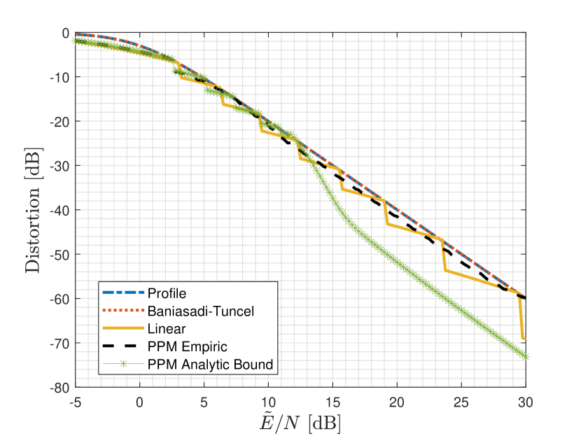
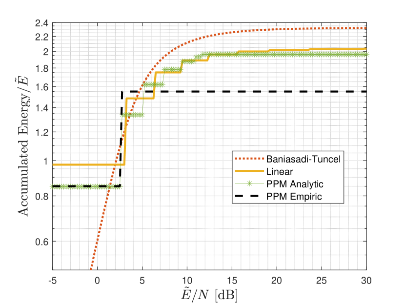
Figure 2: Distortion and accumulated energy of the layers utilized by the receiver at a given $\tilde{E}/N$ for a Gaussian source in the infinite-blocklength regime for a quadratic profile: Sch. V.1 with linear layers with energy allocation $E_{i}=\Delta\mathrm{e}^{-\alpha i}$ for $\Delta=0.975,\alpha=0.65$, empirical performance of the scheme with a linear layer with energy $E_{1}=0.85$ and an analog PPM layer with energy $E_{2}=0.75$, analytic performance of the scheme of Th. V.2 with the parameters from its proof and analytic performance of Baniasadi and Tuncel scheme according to the proof in [17]

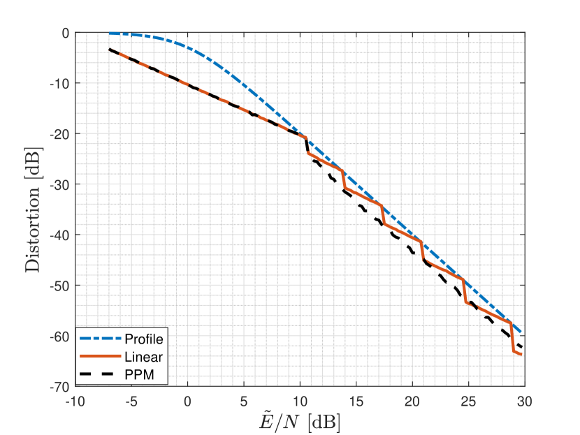
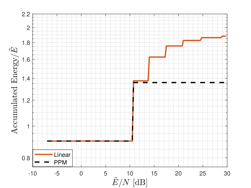
Figure 3: Distortion and accumulated energy of the layers utilized by the receiver at a given $\tilde{E}/N$ for a uniform scalar source for a quadratic profile: Sch. V.1 with linear layers with energy allocation $\frac{E_{i}}{\tilde{E}}=\Delta\mathrm{e}^{-\alpha i}$ for $\Delta=0.9,\alpha=0.64$, and with a linear layer with energy $E_{1}=0.9\tilde{E}$ and an analog PPM layer with energy $E_{2}=0.346\tilde{E}$.

We first consider the infinite-blocklength regime ($k\to\infty$) for a Gaussian source and a quadratic profile [$L=2$ in (3)], for which we have derived analytical guarantees in Secs. V-A and V-B. Fig. 2 depicts the accumulated energy of the employed layers at the receiver of Sch. V and the achievable distortion at a given $\tilde{E}/N$, along with the desired quadratic distortion profile (3b) (with $L=2$) for $N_{\min}\to 0$ for: linear layers, and $M-1$ linear layers with a final analog PPM layer (analytic performance for $M=7$ layers according to Th. V.2 and empirical performance for $M=2$ layers). This figure clearly demonstrates the gain due to introducing an analog PPM layer. Interestingly, the empirical curve shows that only two layers are needed when the second layer is an analog PPM one, meaning that the seven layers needed in the proof of Th. V.2 are an artifact of the slack in our analytic bounds. To derive the performance of the scheme with linear layers we evaluated (85) directly for the optimized energy allocation $E_{i}=\Delta\mathrm{e}^{-\alpha i}$ with $\Delta=0.975$ and $\alpha=0.65$. To derive the analytical performance of Th. V.2, we used the energy allocation from its proof in App. D, while for the empirical performance, optimizing over the energy allocation yielded $E_{1}=0.975\tilde{E},E_{2}=0.5904\tilde{E}$.

We move now to the uniform scalar source setting ($k=1$) and a quadratic profile. The analysis of Sch. V in the scalar setting is difficult. We therefore evaluate its performance empirically for both variants of the scheme: with linear layers, and with one linear layer and one analog PPM layer (two layers suffice in this setting as well). In Fig. 3, we depict again the accumulated energy of the employed layers at the receiver of Sch. V and the achievable distortion at a given $\tilde{E}/N$ for both variants of the scheme, along with the desired quadratic distortion profile (3b) (with $L=2$) for $N_{\min}\to 0$.

VII Summary and Discussion

In this work, we studied the problem of JSCC over an energy-limited channel with unlimited bandwidth and/or transmission time when the noise level is unknown at the transmitter. We showed that MLM-based schemes outperform the existing schemes thanks to the improvement in the performance of all layers (including preceding layers that act as SI) with the ENR. By replacing (some of the) linear layers with analog PPM ones, further improvement was achieved. We further demonstrated numerically that the MLM-layered scheme works well in the scalar-source regime.

We also note that a substantial gap remains between the lower bound in (4) and the upper bound of Th. V.2 for the energy required to achieve a quadratic profile [(3b) with $L=2$]. In Sec. VIII several ways to close this gap are described.

We note that, although we assumed that both the bandwidth and the time are unlimited, the scheme and analysis presented in this work carry over to the setting where one of the two is bounded as long as the other one is unlimited, with little adjustment.

VIII Future Research

Consider first the remaining gap between the lower and upper bounds. As demonstrated in Sec. VI, the upper (achievability) bound on the performance of analog PPM is not tight and calls for further improvement thereof. This step is currently under intense investigation, along with improvement via companding of the presented analog PPM variant in this work as well as via other choices of energy allocation (see Rem. V.4). Furthermore, the optimization was performed numerically and for a particular form of noise levels of an exponential form (recall Rem. V.4). We believe that a systematic optimization procedure could put light on the weaknesses of our scheme and provide further improvement of the overall performance. On the other hand, the outer bounds of [17] are based on specific choices of sequences of noise levels. Therefore, further improvement might be achieved by other choices and calls for further research.

We have also shown that the MLM scheme performs well in the scalar-source regime; it would be interesting to derive analytical performance guarantees for this regime.

Finally, since MLM utilizes well source SI at the receiver and channel SI at the transmitter [11, 12], [13, Chs. 10–12], the proposed scheme can be extended to limited-energy settings such as universal transmission with universal SI at the receiver [31] and the dual problem of the one considered in this work of universal transmission with near-zero bandwidth [32].

Appendix A Proof of Cor. IV.2

To prove Cor. IV.2, we repeat the steps of the proof of Th. IV.1 in [20, Prop. 2]; we next detail the contributions to the small-distortion [20, Eq. (25)] and the large-distortion [20, Eq. (27)] terms due to the deviation (52) from the source p.d.f. from Gaussianity, which are denoted by $d_{S}$ and $d_{L}$, respectively.

We start by bounding the contribution to the small-distortion term. To that end, note that [20, Eqs. (24b) and (25b)] remain unaltered since the decoder remains the same. The contribution to the small-distortion term is bounded from above as follows.

$$\frac{d_{S}}{{\epsilon}} \leq\frac{2}{\beta^{2}}\cdot\int_{\sqrt{2\beta\mathrm{ENR}}}^{\infty}\delta_{f}(a)da$$ (65a)

$$\leq\frac{2}{\beta^{2}}$$ (65b)

where (65a) follows from [20, Eqs. (24b) and (25b)], and (65b) follows from $\delta_{f}$ being non-negative with unit integral.

We next bound the contribution $d_{L}$ to the large distortion term. To that end, note that [20, Eqs. (27) and (28)] remain unaltered since the decoder remains the same. We define by $a_{i}$ the deviation in $\Pr\left(A_{i}\right)$ in [20, Eq. (30)]. Then,

$$\frac{a_{i}}{{\epsilon}} \leq\int_{-\left(\frac{2\mathrm{ENR}\beta}{i}+\frac{i}{2\beta}\right)}^{\infty}\delta_{f}(a)\Bigg{\{}\frac{\sqrt{3}}{4\pi}\mathrm{e}^{-\frac{\ell^{2}(a)}{3}}\!+\left(\frac{1}{\sqrt{8}}+\frac{\ell(a)}{4\sqrt{\pi}}\right)\mathrm{e}^{-\frac{\ell^{2}(a)}{4}}$$

$$\quad+\mathrm{e}^{-\frac{\ell^{2}(a)}{2}}\Bigg{\}}da+\int_{-\infty}^{-\left(\frac{2\mathrm{ENR}\beta}{i}+\frac{i}{2\beta}\right)}\delta_{f}(a)da$$ (66a)

$$\leq\frac{\sqrt{2\mathrm{ENR}}\beta}{i}\int_{0}^{\infty}\delta_{f}\left(\frac{\sqrt{2\mathrm{ENR}}\beta}{i}u-\frac{2\mathrm{ENR}\beta}{i}-\frac{i}{2\beta}\right)$$

$$\ \qquad\quad\!\Bigg{\{}\frac{\sqrt{3}}{4\pi}\mathrm{e}^{-\frac{u^{2}}{3}}+\mathrm{e}^{-\frac{u^{2}}{2}}+\left(\frac{1}{\sqrt{8}}+\frac{u}{4\sqrt{\pi}}\right)\mathrm{e}^{-\frac{u^{2}}{4}}\Bigg{\}}du$$

$$\qquad\quad+\frac{H}{\left(1+\frac{2\mathrm{ENR}\beta}{i}+\frac{i}{2\beta}\right)^{4}}$$ (66b)

$$\leq\frac{\tilde{H}}{\left(1+\frac{2\mathrm{ENR}\beta}{i}+\frac{i}{2\beta}\right)^{4}}\,,$$ (66c)

where (66a) follows from [20, Eqs. (28) and (30)], (66b) follows from integration by substitution and (53), and (66c) follows from (53) for some $\tilde{H}>0$.

By substituting the bound of (66) in [20, Eq. (31)], we may bound $d_{L}$ from above by

$$\frac{d_{L}}{{\epsilon}} \leq 2\sum_{i=2}^{\infty}\left(\frac{i}{\beta}\right)^{2}a_{i}$$ (67)

$$\leq\sum_{i=2}^{\infty}\left(\frac{i}{\beta}\right)^{2}\frac{\tilde{H}}{\left(1+\frac{2\mathrm{ENR}\beta}{i}+\frac{i}{2\beta}\right)^{4}}$$ (68)

$$\leq\tilde{C}$$ (69)

for some $\tilde{C}<\infty$.

Therefore, by (65) and (67), the overall contribution $d$ to the distortion due to the deviation (52) is bounded from above by

$$d =d_{L}+d_{S}$$ (70)

$$\leq{\epsilon}\left(\frac{2}{\beta^{2}}+\tilde{C}\right);$$ (71)

choosing $C=\frac{2}{\beta^{2}}+\tilde{C}<\infty$ concludes the proof.

Appendix B Full version of Sch. V.1

We now present the full multi-layer transmission scheme (cf. Sch. V.1), which includes interleaving and Gaussianization steps, as discussed in Rems. V.1 and V.2, respectively. Block diagrams of the overall scheme and the new ingredients are provided in Figs. 4 and 5, respectively. The new components in Sch. B.1 compared to those in Sch. V.1 (and Fig. 1(a)) are highlighted in green in Fig. 4.

Figure 4: Block diagram of Sch. B.1.

(a) Interleaved MLM Tx_i ($\Pi$MLM_i)

(b) Deinterleaved MLM Rx_i ($\Pi^{-1}$MLM_i)

Figure 5: Block diagram for the i’th MLM layer transmitter and receiver of Sch. B.1. We denote the interleaving and deinterleaving operations by $\Pi$ and $\Pi^{-1}$, respectively.

Scheme B.1 (Full MLM-based).

$M$-Layer Transmitter:

First layer ($i=1$):

• For $B\geq k$, $B\in\mathbb{N}$, accumulates $B^{k}$ source (column) vectors $x^{k}(1),x^{k}(2),\ldots,x^{k}(B^{k})$. Denote by $\mathcal{X}$ the matrix whose columns are the source vectors:

  $$\mathcal{X}\triangleq\begin{bmatrix}x^{k}(1)&x^{k}(2)&\ldots&x^{k}(B^{k})\end{bmatrix}.$$ (72)

• For each $b\in\{1,2,\ldots,B^{k}\}$, transmits each of the entries of the vector $x^{k}(b)$ over the channel (6) linearly (39):

  $$s_{1;\ell,b}(t) \triangleq s\left(t+\left(\ell-1\right)T+\left(b-1\right)kT\right)$$ (73)

  $$=\sqrt{\frac{E_{1}}{T}}\frac{x_{\ell}(b)}{\sigma_{x}}\varphi(t),\qquad t\in[0,T),$$ (74)

  for $\ell=\{1,2,\ldots,k\}$, where $\varphi$ is a continuous unit-norm (i.e., unit-energy) waveform that is zero outside the interval $[0,T]$, say $\phi$ of (43), $E_{1}\in[0,E]$ is the allocated energy for layer $1$, and $E$ is the total available energy of the scheme.

Other layers: For each $i\in\{2,\ldots,M\}$:

• For each $b\in\{1,2,\ldots,B^{k}\}$, calculates the $k$-dimensional tuple

  $$m^{k}_{i}(b) =[\eta_{i}(b)x^{k}(b)+d^{k}_{i}(b)]_{\Lambda}\,,$$ (75)

  where $m^{k}_{i}(b)=\left(m_{i;1}(b),m_{i;2}(b),\ldots,m_{i;k}(b)\right)^{\dagger}$, and $m_{i;\ell}(b)$ denotes the $\ell^{\text{th}}$ entry of $m^{k}_{i}(b)$ for $\ell\in\{1,\ldots k\}$; $\eta_{i}(b)$, $d^{k}_{i}(b)$ and $\Lambda$ take the roles of $\eta,d^{k}$ and $\Lambda$ of Sch. III.1, and are tailored for each layer $i$; $\Lambda$ is chosen to have unit second moment.

• For each $\ell\in\{1,\ldots,k\}$, interleaves the entries $m_{i;\ell}(1),\ldots,m_{i;\ell}(B^{k})$, stacks them into vectors of size $B$, and applies to each of them a $B$-dimensional orthogonal matrix $H_{i}$, as follows.

  $${\tilde{m}}^{B}_{i;(\ell,j)}$$ (76a)

  $$\!=H_{i}\begin{pmatrix}m_{i;\ell}\left(\left\lfloor\frac{j-1}{B^{\ell}}\right\rfloor\cdot B^{\ell+1}+[j-1]_{B^{\ell}}+1\right)\\ m_{i;\ell}\left(\left\lfloor\frac{j-1}{B^{\ell}}\right\rfloor\cdot B^{\ell+1}+[j-1]_{B^{\ell}}+B^{\ell}+1\right)\\ m_{i;\ell}\left(\left\lfloor\frac{j-1}{B^{\ell}}\right\rfloor\cdot B^{\ell+1}+[j-1]_{B^{\ell}}+2B^{\ell}+1\right)\\ \vdots\\ m_{i;\ell}\left(\left\lfloor\frac{j-1}{B^{\ell}}\right\rfloor\cdot B^{\ell+1}+\ [j-1]_{B^{\ell}}+B^{\ell}\left(B-1\right)+1\right)\end{pmatrix}$$ (76b)

  $$\!\triangleq H_{i}\grave{m}^{B}_{i;(\ell,j)}$$ (76c)

  for $j\in\{1,2,\ldots,B^{k-1}\}$, where $\grave{m}^{B}_{i;(\ell,j)}$ is the vector after interleaving; ${\tilde{m}}^{B}_{i;(\ell,j)}$ is the vector after interleaving and matrix multiplication and its $\xi^{\text{th}}$ entry is ${\tilde{m}}_{i;\xi,(\ell,j)}$ for $\xi\in\{1,\ldots,B\}$; the length of the vectors $\grave{m}^{B}_{i;(\ell,j)}$ and ${\tilde{m}}^{B}_{i;(\ell,j)}$ is $B$. Note that the interleaving operation creates doubly-indexed vectors, where a set of $B^{k}$ vectors of length $k$ is transformed into $k\times B^{k-1}$ vectors of length $B$, which are indexed by $\ell\in\{1,\ldots,k\}$ and $j\in\left\{1,\ldots,B^{k-1}\right\}$.

• For each $\ell$, $j$, and $\xi$, views ${\tilde{m}}_{i;\xi,(\ell,j)}$ as a scalar source sample, and generates a corresponding channel input $\left\{s_{i;\xi,(\ell,j)}(t)\middle|t\in[0,T)\right\}$ where

  $$s_{i;\xi,(\ell,j)}(t)$$ (77)

  $$\triangleq\!s\big{(}t+\big{(}(\ell-1)+(\xi-1)k+(j-1)Bk+(i-1)kB^{k}\big{)}T\big{)}$$

  using a scalar JSCC scheme with a predefined energy $E_{i}\geq 0$ that is designed for a predetermined $\mathrm{ENR}_{i}$, or equivalently, $N_{i}=E_{i}/\mathrm{ENR}_{i}$, such that $\sum_{i=1}^{M}E_{i}=E$ and $N_{2}>N_{3}>\cdots>N_{M}>0$.

Receiver: Receives the channel output signal $r$ (6) and recovers the different layers as follows.

First layer ($i=1$): For each $\ell\in\{1,\ldots,k\}$, $b\in\{1,\ldots,B^{k}\}$:

• Recovers the MMSE estimate ${\hat{x}}_{1;\ell}(b)$ of $x_{\ell}(b)$ given $\left\{r_{1;\ell,b}(t)|t\in[0,T)\right\}$, where

  $$r_{1;\ell,b}(t)\triangleq r\left(t+(\ell-1)T+(b-1)kT\right).$$ (78)

  Denote the matrix whose columns comprise these estimates by $\hat{\mathcal{X}}_{1}\triangleq\begin{bmatrix}{\hat{x}}^{k}_{1}(1)&\ldots&{\hat{x}}^{k}_{1}(B^{k})\end{bmatrix}$.

• If the true noise level $N$ satisfies $N>N_{2}$, sets the final estimate $\hat{\mathcal{X}}$ of $\mathcal{X}$ to $\hat{\mathcal{X}}_{1}$ and stops. Otherwise, determines the maximal layer index $\jmath$ for which $N\leq N_{\jmath}$ and continues to process the other layers.

Other layers: For each $i\in\{2,\ldots,\jmath\}$ in ascending order:

• For each $\ell\in\{1,\ldots,k\},\ j\in\{1,\ldots,B^{k-1}\}$ and $\xi\in\{1,\ldots,B\}$, uses the receiver of the scalar JSCC scheme to generate an estimate $\hat{\tilde{m}}^{B}_{i;(\ell,j)}$ of ${\tilde{m}}^{B}_{i;(\ell,j)}$ from $\left\{r_{i;\xi,(\ell,j)}(t)\middle|t\in[0,T)\right\}$, where

  $$r_{i;\xi,(\ell,j)}(t)$$ (79)

  $$\triangleq r\left(t+\left((\ell-1)+(\xi-1)k+(j-1)Bk+(i-1)kB^{k}\right)T\right).$$

• For each $\ell\in\{1,\ldots,k\}$, stacks the entries of $\hat{\tilde{m}}^{B}_{i;(\ell,1)},\ldots,\hat{\tilde{m}}^{B}_{i;(\ell,B^{k-1})}$ into vectors of length $B$, $\hat{\tilde{m}}^{B}_{i;(\ell,j)}$, applies the orthogonal matrix $H_{i}^{-1}=H_{i}^{\dagger}$ to each vector $\hat{\tilde{m}}^{B}_{i;(\ell,j)}$, and deinterleaves the outcomes, to attain $\hat{\grave{m}}^{B}_{i;(\ell,j)}$, as follows.

  $$\hat{\grave{m}}^{B}_{i;(\ell,j)}$$ (80a)

  $$=\begin{pmatrix}\hat{m}_{i;\ell}\left(\left\lfloor\frac{j-1}{B^{\ell}}\right\rfloor\cdot B^{\ell+1}+[j-1]_{B^{\ell}}\right)\\ \hat{m}_{i;\ell}\left(\left\lfloor\frac{j-1}{B^{\ell}}\right\rfloor\cdot B^{\ell+1}+[j-1]_{B^{\ell}}+B^{\ell}\right)\\ \hat{m}_{i;\ell}\left(\left\lfloor\frac{j-1}{B^{\ell}}\right\rfloor\cdot B^{\ell+1}+[j-1]_{B^{\ell}}+2B^{\ell}\right)\\ \vdots\\ \hat{m}_{i;\ell}\left(\left\lfloor\frac{j-1}{B^{\ell}}\right\rfloor\cdot B^{\ell+1}+[j-1]_{B^{\ell}}+B^{\ell}\left(B-1\right)\right)\end{pmatrix}\qquad$$ (80b)

  $$=H_{i}^{\dagger}\hat{\tilde{m}}^{B}_{i;(\ell,j)}$$ (80c)

  for $j\in\left\{1,2,\ldots,B^{k-1}\right\}$.

• For each $b\in\left\{1,\ldots,B^{k}\right\}$, using the effective channel output $\hat{m}_{i}^{k}(b)$ (that takes the role of $y^{k}$ in Sch. III.1) with SI ${\hat{x}}_{i-1}^{k}(b)$, generates the signal

  $$\tilde{y}^{k}_{i}(b) =[\alpha^{(i)}_{c}\hat{m}^{k}_{i}(b)-\eta_{i}{\hat{x}}^{k}_{i-1}(b)-d^{k}_{i}(b)]_{\Lambda},$$ (81)

  as in (18) of Sch. III.1, where $\alpha^{(i)}_{c}$ is a channel scale factor.

• For each $b\in\left\{1,\ldots,B^{k}\right\}$, constructs an estimate ${\hat{x}}^{k}(b)$ of $x^{k}(b)$:

  $${\hat{x}}_{i}^{k}(b) =\frac{\alpha^{(i)}_{s}}{\eta_{i}}\tilde{y}^{k}_{i}(b)+{\hat{x}}^{k}_{i-1}(b),$$ (82)

  as in (19) of Sch. III.1, where $\alpha^{(i)}_{s}$ is a source scale factor. Denote the matrix whose columns comprise these estimates by $\hat{\mathcal{X}}_{i}\triangleq\begin{bmatrix}{\hat{x}}^{k}_{i}(1)&\ldots&{\hat{x}}^{k}_{i}(B^{k})\end{bmatrix}$. The final estimate is $\hat{\mathcal{X}}=\hat{\mathcal{X}}_{\jmath}$.

Appendix C Proof of Th. V.1

To prove Th. V.1, we will make use of the following lemma about the validity of the MLM results from Sec. III for the multi-layer MLM scenario, where the mid-stage noise vectors are linear combinations of dithers and Gaussian noises. The proof of this lemma is given in App. E.

Lemma C.1.

Let $q^{k}$ be a sequence in $k$ of vectors, such that the vector $q^{k}$ equals with probability $1-P_{k}$ to a linear combination of a Gaussian vector and dithers all of which are mutually independent, where $\lim_{k\to\infty}P_{k}=0$. Then, the sequence in $k$ of error signals $x^{k}-{\hat{x}}^{k}$ is SNE for a sequence of lattices that is good for both channel coding and MSE quantization; moreover, for each $k$, the error signal equals with probability $1-Q_{k}$ to a linear combination of a Gaussian vector and dithers all of which are mutually independent, where $\lim_{k\to\infty}Q_{k}=0$.

We now prove Th. V.1. We will construct a scheme with a large enough (yet finite) $M$ that achieves (3b) with the predefined $L$ and $\tilde{E}$ for all $N>N_{\min}$ for a given $N_{\min}>0$. For any $N_{\min}>0$, however small, we will choose $M\in\mathbb{N}$ large enough and $\{N_{i}|i=1,\ldots,M\}$ such that $N_{\min}\in(N_{M},N_{M-1}]$.

Consider the first layer ($i=1$). The distortion $D_{1}$ of ${\hat{x}}_{1}^{k}$ for a noise level $N$ is bounded from above by

$$D_{1}(N) =\frac{\sigma^{2}_{x}}{1+\frac{2E_{1}}{N}}$$ (83a)

$$\leq\sigma_{x}^{2}\cdot\mathcal{F}(N)$$ (83b)

$$=\frac{\sigma_{x}^{2}}{1+\left(\frac{\tilde{E}}{N}\right)^{L}}$$ (83c)

where (83a) follows from (41), and (83b) and (83c) follow from the distortion profile requirement (3) for $N>N_{2}$.

To guarantee the requirement (83b) for all $N>N_{2}$, it suffices to guarantee it for the extreme value $N=N_{2}$, which holds, in turn, for

$$E_{1} =\left(\frac{\tilde{E}}{N_{2}}\right)^{L}\frac{N_{2}}{2}.$$ (84)

For $i\in\{2,\ldots,\jmath\}$, the distortion $D_{i}$ of ${\hat{x}}_{i}^{k}$ for a noise level $N$ is bounded from above by

$$D_{i}(N) \leq\frac{D_{i-1}(N_{i})}{1+\frac{2E_{i}}{N}}\cdot\frac{1+\frac{2E_{i}}{N_{i}}}{\frac{2E_{i}}{N_{i}}}+{\epsilon}_{i}$$ (85a)

$$\leq\frac{\sigma_{x}^{2}\cdot\mathcal{F}(N_{i})}{1+\frac{2E_{i}}{N}}\cdot\frac{1+\frac{2E_{i}}{N_{i}}}{\frac{2E_{i}}{N_{i}}}+{\epsilon}_{i}$$ (85b)

$$=\frac{\sigma_{x}^{2}}{1+\left(\frac{\tilde{E}}{N_{i}}\right)^{L}}\cdot\frac{1}{1+\frac{2E_{i}}{N}}\cdot\frac{1+\frac{2E_{i}}{N_{i}}}{\frac{2E_{i}}{N_{i}}}+{\epsilon}_{i}$$ (85c)

$$\leq\sigma_{x}^{2}\cdot\mathcal{F}(N)$$ (85d)

$$=\frac{\sigma_{x}^{2}}{1+\left(\frac{\tilde{E}}{N}\right)^{L}},$$ (85e)

where (85a) follows from Cor. III.2 by treating ${\hat{x}}_{i-1}^{k}$ as SI and the error $x-{\hat{x}}_{i-1}^{k}$ taking the role of the “unknown part” at the receiver with power $D_{i-1}$, with ${\epsilon}_{i}$ going to zero with $k$, and by invoking Lem. C.1 recursively, which guarantees that the sequence in $k$ of the error vectors $x-{\hat{x}}_{i-1}^{k}$ is SNE; (85b) holds by the distortion profile requirement (3); (85c) follows from (3b) with $\tilde{E}$ and $L$; (85d) follows from the distortion profile requirement (3) for $N\in(N_{i+1},N_{i}]$; and (85e) follows from (3b) with $\tilde{E}$ and $L$.

To guarantee the requirement (85d) for all $N\in(N_{i+1},N_{i}]$ we need only to satisfy it for the extreme value $N=N_{i+1}$, which holds, in turn, for

$$1+\frac{2E_{i}}{N_{i+1}} \geq\frac{1+\frac{2E_{i}}{N_{i}}}{\frac{2E_{i}}{N_{i}}}\cdot\frac{1+\left(\frac{\tilde{E}}{N_{i+1}}\right)^{L}}{1+\left(\frac{\tilde{E}}{N_{i}}\right)^{L}}+{\tilde{{\epsilon}}}_{i}$$ (86a)

$$\geq\left(1+\frac{N_{i}}{2E_{i}}\right)\left(\frac{N_{i}}{N_{i+1}}\right)^{L}+{\tilde{{\epsilon}}}_{i},$$ (86b)

where (86b) holds since $N_{i+1}<N_{i}$. and ${\tilde{{\epsilon}}}_{i}$ decays to zero with $k$; the set of inequalities (86) holds for

$$E_{i} =\frac{N_{i+1}}{4}\left(\left(\frac{N_{i}}{N_{i+1}}\right)^{L}\!-1\right)\left(1+\!\sqrt{1+\frac{4\left(\frac{N_{i}}{N_{i+1}}\right)^{L+1}}{\left(1-\left(\frac{N_{i}}{N_{i+1}}\right)^{L}\right)^{2}}}\right)+\varepsilon_{i},$$ (87)

where again $\varepsilon_{i}$ decay to zero with $k$.

We are now ready to bound the total energy $E$.

$$\frac{E}{\tilde{E}}=\frac{1}{\tilde{E}}\sum_{i=1}^{\jmath}E_{i}$$ (88a)

$$\leq\sum_{i=2}^{\infty}\frac{N_{i+1}}{4\tilde{E}}\left(\left(\frac{N_{i}}{N_{i+1}}\right)^{L}-1\right)\left(1+\sqrt{1+\frac{4\left(\frac{N_{i}}{N_{i+1}}\right)^{L+1}}{\left(1-\left(\frac{N_{i}}{N_{i+1}}\right)^{L}\right)^{2}}}\right)$$

$$\qquad\qquad+\frac{1}{2}\left(\frac{\tilde{E}}{N_{2}}\right)^{L-1}+\sum_{i=2}^{\jmath}\frac{\varepsilon_{i}}{\tilde{E}}$$ (88b)

$$=\frac{\Delta}{4\tilde{E}}\left(\mathrm{e}^{\alpha L}-1\right)\left(1+\sqrt{1+\frac{4\mathrm{e}^{\alpha\left(L+1\right)}}{\left(1-\mathrm{e}^{\alpha L}\right)^{2}}}\right)\sum_{i=2}^{\infty}\mathrm{e}^{-\alpha i}$$ (88c)

$$\qquad\qquad+\frac{1}{2}\left(\frac{\tilde{E}}{\Delta\mathrm{e}^{-\alpha}}\right)^{L-1}+\sum_{i=2}^{\jmath}\frac{\varepsilon_{i}}{\tilde{E}}$$ (88d)

$$=\frac{x}{4}\left(\mathrm{e}^{\alpha L}-1\right)\left(1+\sqrt{1+\frac{4\mathrm{e}^{\alpha\left(L+1\right)}}{\left(1-\mathrm{e}^{\alpha L}\right)^{2}}}\right)\frac{\mathrm{e}^{-2\alpha}}{1-\mathrm{e}^{-\alpha}}$$ (88e)

$$\qquad\qquad+\frac{1}{2}\left(\frac{\mathrm{e}^{\alpha}}{x}\right)^{L-1}+\sum_{i=2}^{\jmath}\frac{\varepsilon_{i}}{\tilde{E}},$$ (88f)

where (88b) follows from (84) and (87), in (88d) we use the choice $N_{i}=\Delta\mathrm{e}^{-\alpha\left(i-1\right)}$ for the noise levels for some positive parameters $\alpha$ and $\Delta$, and (88f) holds by defining $x\triangleq\Delta/\tilde{E}$.

Finally, by optimizing over the parameters $\alpha$ and $x$, taking a large enough $M$, and taking $k$ to infinity, we arrive at the desired result.

For the particular case of a quadratically decaying profile ($L=2$), numerically optimizing (88f) over $\alpha$ and $x$ yields (63).

Appendix D Proof of Th. V.2

To prove Th. V.2, we will make use of the following non-uniform variant of the Berry–Esseen theorem, which is a weakened (yet more compact) form of a result due to Petrov.

Theorem D.1 (​​[33], [34, Ch. VII, Thm. 17]).

Let $\{x_{i}|i\in\mathbb{N}\}$ be an i.i.d. sequence of RVs with zero mean and unit variance, and denote $s_{n}\triangleq\frac{1}{\sqrt{n}}\sum_{i=1}^{n}x_{i}$. Assume that $\mathbb{E}\left[|x_{1}|^{\nu}\right]<\infty$ for some $\nu>2$, and that $x_{1}$ has a bounded p.d.f. Then, the p.d.f. of $s_{n}$, denoted by $f_{n}$, satisfies

$$\left|f_{n}(a)-f_{G}(a)\right| <\frac{A_{\nu}}{\sqrt{n}\cdot\left(1+|a|^{\nu}\right)}, \forall a \in\mathbb{R},$$ (89)

for some $A_{\nu}<\infty$, where $f_{G}$ is the standard Gaussian p.d.f.

Furthermore, as discussed in Rems. V.1–V.3, in each layer (and specifically in the PPM layer) we effectively have an additive noisy channel whose noise distribution approaches a Gaussian distribution (due to the Gaussianization and the interleaving). For all the linear layers, Lem. C.1 allow us to use the MLM results of Sec. III. However, for the PPM layer, instead of a combination of Gaussian vectors and dithers (as treated in Lem. C.1) the actual noise contains also terms that are induced by the PPM scheme. We will use the following lemma, which is proved in App. F, to claim that the effect of these terms on the performance of the MLM scheme can be made arbitrarily small, by taking the dimension $k$ to be large enough.

Lemma D.1.

Let $x^{k}$ be a sequence in $k$ of SNE vectors with second moment $r_{k}$ such that $\lim_{k\to\infty}r_{k}=r$, and let ${\hat{x}}^{k}$ be a corresponding sequence in $k$ of vectors with identically distributed entries such that:

• The distance between the p.d.f. of $x_{1}$ and that of ${\hat{x}}_{1}$ is bounded from above by

  $$\left|f_{{\hat{x}}_{1}}(t)-f_{x_{1}}(t)\right| \leq\frac{C(t)}{\sqrt{k}} \forall t>0,$$ (90)

  where $C(t)=o\left(1/t^{2}\right)$, and where $x_{1}$ and ${\hat{x}}_{1}$ denote the first entries of the vectors $x^{k}$ and ${\hat{x}}^{k}$, respectively.

• The correlation between any two squared entries within ${\hat{x}}^{k}$ decays to zero with $k$, viz..,

  $$\lim_{k\to\infty}\mathrm{cov}\left({\hat{x}}^{2}_{i},{\hat{x}}^{2}_{j}\right)=0,$$ (91)

  where $\mathrm{cov}\left(A,B\right)\triangleq\mathbb{E}\left[AB\right]-\mathbb{E}\left[A\right]\mathbb{E}\left[B\right]$ denotes the covariance of $A$ and $B$.

Then, for all $\epsilon,\delta>0$, there exists $k_{0}\in\mathbb{N}$ such that

$$P\left(\frac{1}{k}\left\|{\hat{x}}^{k}\right\|^{2}>r+\delta\right)\leq\epsilon$$ (92)

for all $k>k_{0}$, namely, the sequence $\left\{{\hat{x}}^{k}\middle|k\in\mathbb{N}\right\}$ is a sequence of SNE vectors.

We will now prove Th. V.2. We note that the following analysis is based on the interleaving and Gaussianization blocks as they appear in the full description of the scheme in App. B.

Proof:

We will now derive the parameters that achieve a quadratic profile ($L=2$) and $\tilde{E}$ in (3b) for all $N>N_{\min}$ for a given $N_{\min}>0$.

We choose $H_{i}=I_{B}$ for the linear layers—layers $i=\{1,2,\ldots,M-1\}$. Consequently, the analysis for the first $M-1$ layers of the proof of Th. V.1 carries over to this scheme as well.

Consider now the last layer—layer $M$. Following Feder and Ingber [27], and Hadad and Erez [28], we use a $B$-dimensional Walsh–Hadamard matrix $H_{M}$.

Now, if $N\in\left(N_{M-1},N_{M}\right]$, the receiver uses the last layer to improve the source estimates while viewing the estimates resulting from the previous layer, $\{{\hat{x}}_{M-1}^{k}(1),\ldots,{\hat{x}}_{M-1}^{k}(B)\}$, as SI with mean power $D_{M-1}(N_{M})$ (85).

By Lem. III.1, all the moments of all the entries of $m_{M}^{k}(b)$ exist and are finite for all $b$. Thus, by Th. D.1, and since $m_{M}^{k}(1),m_{M}^{k}(2),\ldots,m_{M}^{k}(B^{k})$ are i.i.d., the p.d.f. $f_{\ell}$ of ${\tilde{m}}_{M;(\ell,j)}(b)$ (it is the same for all $b$ and $j$ for a given $\ell$) satisfies

$$|f_{\ell}(a)-f_{G_{\ell}}(a)|<\frac{A_{\nu}}{\sqrt{B}\left(1+|a|^{\nu}\right)}$$ (93)

for all $\ell\in\{1,\ldots,k\}$, $b\in\{1,\ldots,B\}$, and $j\in\{1,2,\ldots,B^{k-1}\}$, for all $\nu>2$ for some $A_{\nu}<\infty$, where $f_{G_{\ell}}$ is the p.d.f. of a zero-mean Gaussian RV with the same variance as ${\tilde{m}}_{M;(\ell,j)}(b)$.

By choosing some $\nu>4$ and applying Cor. IV.2 to ${\tilde{m}}_{M;\ell}(b)$ with $h(a)=A_{\nu}/\left(1+|a|^{\nu}\right)$ and ${\epsilon}=1/\sqrt{B}$, the distortion bound of Th. IV.1 is attained up to a loss $C/\sqrt{B}$ for some constant $C<\infty$, where this loss can be made arbitrarily small by choosing a large enough $B$.

We note that the interleaving makes the PPM transmitters operate over elements that are related to lattices of different sources. Thus, after deinterleaving, the correlation between different vector elements, as well as the correlation between their squares, vanishes as $k\to\infty$. Furthermore, the per-element variance is bounded from above by quantity that approaches (as $k\to\infty$) the PPM performance bound of Th. IV.1. Thus, by Lem. D.1, the resulting effective noise vector $z_{\mathrm{eff}}^{k}=\hat{m}_{M}^{k}(b)-m_{M}^{k}(b)$ is SNE (recall Def. III.1).

We note that $z_{\mathrm{eff}}^{k}(b)$ is correlated with $m_{M}^{k}(b)$; nevertheless, by Cor. III.4 with parameters ${\tilde{\alpha}}=\alpha_{c}=\alpha_{s}=1$ the distortion of ${\hat{x}}_{M}^{k}$ is bounded from above by

$$D_{M}(N)\leq\frac{D_{M-1}(N_{M})}{\mathrm{SDR}_{M}\left(N\right)}+{\epsilon}_{M},$$ (94)

where ${\epsilon}_{M}$ subsumes the aforementioned losses that all go to zero with $k$, and $\mathrm{SDR}_{M}(N)$ is the SDR of the analog PPM scheme for a noise power $N$ of Th. IV.1.

The energy $E_{M}$ of the last layer is chosen to comply with the profile for $N<N_{M}$:

$$D_{M}\left(N\right) \leq\mathcal{F}\left(N\right) \forall N<N_{M}.$$ (95)

Combining (94) and the contribution of the first $M-1$ layers, given by (88d) with summation from $1$ to $M-1$. By numerically optimizing the resulting term over the number of layers $M$, the PPM pulse width $\beta$ and the energy layers $\left\{E_{i}\right\}_{i=1}^{M}$ we obtain that $M=7$, $\beta=0.9$ and the layer energies $E_{1}\approx 0.8480\tilde{E},E_{2}\approx 0.4893\tilde{E},E_{3}\approx 0.2823\tilde{E},E_{4}\approx 0.1629\tilde{E}$, $E_{5}\approx 0.094\tilde{E}$, $E_{6}\approx 0.0542\tilde{E}$, $E_{7}\approx 0.0313\tilde{E}$ yields (64). ∎

Appendix E Proof of Lem. C.1

Since $\Lambda^{(k)}$ is assumed to be a sequence that is good for channel coding,

$$\lim_{k\to\infty}\Pr\left(x^{k}-{\hat{x}}^{k}=e^{k}\right)=1,$$ (96)

where $e^{k}\triangleq(1-\alpha_{s})q^{k}-\frac{\alpha_{s}\alpha_{c}}{\beta}z^{k}+\frac{\alpha_{s}\left(1-\alpha_{c}\right)}{\beta}m^{k}$; equivalently, for any ${\epsilon}_{1}>0$, however small, there exists $k_{1}\in\mathbb{N}$, such that for all $k>k_{1}$,

$$\Pr\left(x^{k}-{\hat{x}}^{k}\neq e^{k}\right)<{\epsilon}_{1}.$$ (97)

Note now that $e^{k}$ equals a linear combination of independent Gaussian vectors—which amounts to a Gaussian vector—and dither vectors. Hence, by [21, Th. 3], the sequence in $k$ of vectors $e^{k}$ is SNE, namely, for any $\delta,{\epsilon}_{2}>0$, however small, there exists $k_{2}\in\mathbb{N}$, such that for all $k>k_{1}$,

$$\Pr\left(\frac{1}{k}\mathbb{E}\left[\left\|e^{k}\right\|^{2}\right]>(1+\delta)\sigma_{e}^{2}\right)\leq{\epsilon}_{2}.$$ (98)

Now let ${\epsilon}>0$, however small and choose ${\epsilon}_{1}={\epsilon}_{2}={\epsilon}/2$, and $k_{0}=\max\{k_{1},k_{2}\}$. Then, by the union bound, for all $k>k_{0}$,

$$\Pr\left(\frac{1}{k}\mathbb{E}\left[\left\|x^{k}-{\hat{x}}^{k}\right\|^{2}\right]>(1+\delta)\sigma_{x-{\hat{x}}}^{2}\right)\leq{\epsilon}.$$ (99)

Appendix F Proof of Lem. D.1

By (90),

$$\left|\mathbb{E}\left[{\hat{x}}^{2}_{1}\right]-\mathbb{E}\left[x_{1}^{2}\right]\right|=\left|\int_{t=\infty}^{\infty}t^{2}\left[f_{{\hat{x}}_{1}}(t)-f_{x_{1}}(t)\right]dt\right|\leq\frac{G}{\sqrt{k}}$$ (100)

where $G$ is a finite constant, since $C(t)=o(t)$, that depends on $C(t)$, and $\mathbb{E}\left[x_{1}^{2}\right]=r_{k}$. Using second-moment ergodicity of the entries of $x^{k}$, which holds in the limit of $k\to\infty$ [35, Thm. 12.1] by (91) and recalling that $\lim_{k\to\infty}r_{k}=r$ concludes the proof.

References

- [1] T. M. Cover and J. A. Thomas, Elements of Information Theory, Second Edition. New York: Wiley, 2006.
- [2] A. El Gamal and Y.-H. Kim, Network Information Theory. Cambridge University Press, 2011.
- [3] C. E. Shannon, “Coding theorems for a discrete source with a fidelity criterion,” in Institute of Radio Engineers, International Convention Record, vol. 7, 1959, pp. 142–163.
- [4] E. Köken and E. Tuncel, “On minimum energy for robust Gaussian joint source–channel coding with a distortion–noise profile,” in Proceedings of the IEEE International Symposium on Information Theory (ISIT), Aachen, Germany, 2017, pp. 1668–1672.
- [5] W. H. R. Equitz and T. M. Cover, “Successive refinement of information,” IEEE Transactions on Information Theory, vol. 37, no. 2, pp. 851–857, Mar. 1991.
- [6] N. Santhi and A. Vardy, “Analog codes on graphs,” in Proceedings of the IEEE International Symposium on Information Theory (ISIT), Yokohama, Japan, 2003, p. 13.
- [7] ——, “Analog codes on graphs,” arXiv preprint cs/0608086, 2006.
- [8] K. Bhattad and K. R. Narayanan, “A note on the rate of decay of mean-squared error with snr for the awgn channel,” IEEE Transactions on Information Theory, vol. 56, no. 1, pp. 332–335, 2010.
- [9] U. Mittal and N. Phamdo, “Hybrid digital-analog (HDA) joint source–channel codes for broadcasting and robust communications,” IEEE Transactions on Information Theory, vol. 48, no. 5, pp. 1082–1102, May 2002.
- [10] Z. Reznic, M. Feder, and R. Zamir, “Distortion bounds for broadcasting with bandwidth expansion,” IEEE Transactions on Information Theory, vol. 52, no. 8, pp. 3778–3788, Aug. 2006.
- [11] Y. Kochman and R. Zamir, “Joint Wyner–Ziv/dirty-paper coding by modulo-lattice modulation,” IEEE Transactions on Information Theory, vol. 55, pp. 4878–4899, Nov. 2009.
- [12] ——, “Analog matching of colored sources to colored channels,” IEEE Transactions on Information Theory, vol. 57, no. 6, pp. 3180–3195, June 2011.
- [13] R. Zamir, Lattice Coding for Signals and Networks. Cambridge: Cambridge University Press, 2014.
- [14] A. D. Wyner and J. Ziv, “The rate–distortion function for source coding with side information at the decoder,” IEEE Transactions on Information Theory, vol. 22, no. 1, pp. 1–10, Jan. 1976.
- [15] A. D. Wyner, “The rate–distortion function for source coding with side information at the decoder—II: General sources,” Information and Control, vol. 38, pp. 60–80, 1978.
- [16] E. Köken and E. Tuncel, “On minimum energy for robust Gaussian joint source–channel coding with a distortion–noise profile,” in Proceedings of the IEEE International Symposium on Information Theory (ISIT), 2017, pp. 1668–1672.
- [17] M. Baniasadi and E. Tuncel, “Minimum energy analysis for robust Gaussian joint source–channel coding with a square-law profile,” in Proceedings of the IEEE International Symposium on Information Theory and Its Applications (ISITA), 2020, pp. 51–55.
- [18] M. Baniasadi, E. Köken, and E. Tuncel, “Minimum energy analysis for robust Gaussian joint source–channel coding with a distortion–noise profile,” IEEE Transactions on Information Theory, vol. 68, no. 12, pp. 7702–7713, Dec. 2022.
- [19] M. Baniasadi, “Robust Gaussian joint source–channel coding with a staircase distortion–noise profile,” CoRR, 2020. [Online]. Available: http://arxiv.org/abs/2001.09370
- [20] O. Lev and A. Khina, “Energy-limited joint source–channel coding via analog pulse position modulation,” IEEE Transactions on Communications, vol. 70, no. 8, pp. 5140–5150, August 2022.
- [21] O. Ordentlich and U. Erez, “A simple proof for the existence of “good” pairs of nested lattices,” IEEE Transactions on Information Theory, vol. 62, no. 8, pp. 4439–4453, 2016.
- [22] Y. Kochman, A. Khina, U. Erez, and R. Zamir, “Rematch-and-forward: Joint source–channel coding for parallel relaying with spectral mismatch,” IEEE Transactions on Information Theory, vol. 60, no. 1, pp. 605–622, 2014.
- [23] U. Erez and R. Zamir, “Achieving on the AWGN channel with lattice encoding and decoding,” IEEE Transactions on Information Theory, vol. 50, no. 10, pp. 2293–2314, Oct. 2004.
- [24] J. M. Wozencraft and I. M. Jacobs, Principles of Communication Engineering. New York: John Wiley & Sons, 1965.
- [25] A. J. Viterbi and J. K. Omura, Principles of Digital Communication and Coding. New York: McGraw-Hill, 1979.
- [26] Y. Wu and S. Verdú, “Functional properties of minimum mean-square error and mutual information,” IEEE Transactions on Information Theory, vol. 58, no. 3, pp. 1289–1301, 2011.
- [27] M. Feder and A. Ingber, “Method, device and system of reduced peak-to-average-ratio communication,” U.S. Patent 11/971,934, Feb. 14, 2014.
- [28] R. Hadad and U. Erez, “Dithered quantization via orthogonal transformations,” IEEE Transactions on Signal Processing, vol. 64, no. 22, pp. 5887–5900, 2016.
- [29] H. Asnani, I. Shomorony, A. S. Avestimehr, and T. Weissman, “Network compression: Worst case analysis,” IEEE Transactions on Information Theory, vol. 61, no. 7, pp. 3980–3995, 2015.
- [30] A. No and T. Weissman, “Rateless lossy compression via the extremes,” IEEE Transactions on Information Theory, vol. 62, no. 10, pp. 5484–5495, 2016.
- [31] M. Baniasadi and E. Tuncel, “Robust Gaussian JSCC under the near-infinity bandwidth regime with side information at the receiver,” in Proceedings of the IEEE International Symposium on Information Theory (ISIT), 2021.
- [32] ——, “Robust Gaussian joint source–channel coding under the near-zero bandwidth regime,” in Proceedings of the IEEE International Symposium on Information Theory (ISIT), 2020, pp. 2474–2479.
- [33] V. V. Petrov, “On local limit theorems for sums of independent random variables,” Theory of Probability & Its Applications, vol. 9, no. 2, pp. 312–320, 1964.
- [34] ——, Sums of Independent Random Variables. New York: Springer-Verlag, 1975.
- [35] A. Papoulis and S. U. Pillai, Probability, random variables, and stochastic processes, 4th ed. Tata McGraw-Hill Education, 2002.