Modelling the stellar halo with RR-Lyrae stars

Abstract

A seven-parameter distribution function (DF) is fitted to $20\,000$ RR-Lyrae stars for which only astrometric data are available. The observational data are predicted by the DF in conjunction with the gravitational potential of a self-consistent model Galaxy defined by DFs for the dark halo, the bulge and a four-component disc. Tests of the technique developed to deal with missing line-of-sight velocities show that adding such velocities tightens constraints on the DF only slightly. The recovered model of the RR-Lyrae population confirms that the population is flattened and has a strongly radially biased velocity distribution. At large radii its density profile tends to $\rho\sim r^{-4.5}$ but no power law provides a good fit inside the solar sphere. The model is shown to provide an excellent fit to the data for stars brighter than $r=16.5$ but at certain longitudes it predicts too few faint stars at Galactocentric radii $\sim 20\,\mathrm{kpc}$, possibly signalling that the halo is not axisymmetric. The DF is used to predict the velocity distribution of BHB stars for which space velocities are available. The $z$ components are predicted successfully but too much anisotropy in the $v_{R}v_{\phi}$ plane is expected.

1 Introduction

Although its mass is relatively small, the stellar halo of our Galaxy is of great interest for several reasons. Among these is the fact that it contains many of the oldest stars in the Galaxy, and it is widely believed that important insights into the Galaxy’s history can be gleaned from the halo’s chemodynamical structure (Bell et al., 2008; Belokurov et al., 2018; Lancaster et al., 2019; Myeong et al., 2019; Belokurov et al., 2020). The stellar halo is also important as a tracer of the Galaxy’s gravitational field. Indeed, the kinematics of disc stars and cool gas have enabled us to map the gravitational field in significant detail near the plane for several kiloparsecs either side of the solar radius $R_{0}$ (Binney et al., 2014; Binney & Piffl, 2015; Cole & Binney, 2017; Bland-Hawthorn & Gerhard, 2016), but the structure of the field far from the plane and beyond $R\sim 1.5R_{0}$ is not tightly constrained. Available tracers of the field at these locations include tidal streams (Koposov et al., 2009; Bovy, 2014; Gibbons et al., 2016; Erkal et al., 2016; Koposov et al., 2019), globular clusters (Binney & Wong, 2017; Vasiliev, 2019b) and dwarf spheroidal satellites (Wilkinson & Evans, 1999), and populations of halo stars (Deason et al., 2011, 2019).

RR-Lyrae stars are probably the most useful population of halo stars because they are quite luminous ($M_{V}\sim 0.5$) so can be detected within a large volume, and their distances can be obtained to excellent precision from their period-luminosity relation. Sesar et al. (2017) used machine-learning to identify $45\,000$ RR-Lyrae stars in photometric data from the PanSTARRS1 survey (Kaiser et al., 2010). Astrometric data for most of these stars are available in the second and third data releases from the European Space Agency’s satellite Gaia (Gaia Collaboration et al., 2018; Gaia Collaboration, 2021). Combining the proper-motion data from Gaia with distances from the PanSTARRS photometry, we obtain precision five-dimensional data for a population that traces the Galaxy’s gravitational field.

Learning how to exploit such five-dimensional data is an interesting and potentially valuable exercise because through parallaxes and proper motions Gaia provides five dimensional data for in excess a billion stars. To date most studies of Galactic structure that use Gaia data restrict attention to the $\la 7$ million stars in the DR2 radial-velocity sample because for these stars one has six-dimensional data. With such data, each star has a fairly well defined location in phase space. Working with five-dimensional data is much more challenging because we are ignorant of the line-of-sight velocities $v_{\parallel}$. Here we develop a technique for managing our ignorance.

A population of tracer objects can be used to constrain the Galaxy’s gravitational field only to the extent that the latter can be approximated by a constant field. Most halo objects are not expected to respond strongly to the Galaxy’s rotating bar or spirals, and the Galaxy’s potential well deepens on a timescale that is too long to invalidate the assumption of instantaneous equilibrium. Within Galactocentric radii that are probed by RR-Lyrae stars, disequilibrium caused by the orbits of the Magellanic Clouds probably also has too long a timescale to be important. The same may not be true of the disequilibrium induced by the Sagittarius dwarf galaxy, but a reasonable strategy seems to be to ignore the Sagittarius dwarf in the first instance and then to use the resulting model to investigate the impact that the Sgr Dwarf has on a population like that of the RR-Lyrae stars.

For these reasons our scheme for exploiting the RR-Lyrae sample is to seek a distribution function (DF) with these objects given the observations and a time-independent and axisymmetric model of the Galaxy’s gravitational field. By Jeans theorem (Jeans, 1915) the DF can be taken to be a function of the isolating integrals of motion in the given gravitational field, and these integrals are most conveniently taken to be three actions: $J_{r}$, which quantifies te amplitude of radial excursions, $J_{z}$, which quantifies oscillations either side of the Galactic plane, and $J_{\phi}$, which is the component of angular momentum parallel to the Galaxy’s assumed symmetry axis. Hence we assume that the DF of the RR-Lyrae stars is an analytic function $f({\bf J})$. The model gravitational field in which the RR-Lyrae stars are assumed to move is that of a self-consistent model Galaxy that is defined by a series of similar DFs, one for each of the principal mass-bearing components of the Galaxy. Specifically, the dark halo, an (axisymmetric) bulge and four disc components: a young disc, a middle-aged disc and an old thin disc plus a high-$\alpha$ disc. The gravitational potential that these DFs jointly generate is found iteratively in the manner originally described by Binney (2014) using the AGAMA package (Vasiliev, 2019a), which computes actions and gravitational potentials with remarkable efficiency, and takes care of the complex book-keeping involved in self-consistent galaxy modelling.

In this paper our focus is on determination of the DF of a sample of tracers for which we have five-dimensional data. Hence we will consider many possible DFs for the sample but use only one gravitational potential, which will arise from, and be defined by, a single set of DFs for the Galaxy’s mass-bearing components. In a subsequent paper we will consider the extent to which data for a tracer population such as the RR-Lyrae stars can be used to constrain the DFs of the mass-bearing populations.

The plan of this paper is as follows. Section 2.1 gives the functional form of the DF we fit, Section 2.2 summarises the general theory of fitting DFs to data for individual stars and Section 2.3 outlines the numerical procedure for evaluating distribution functions. Section 2.4 explains how correlations between parallax and proper motion in Gaia data can be used to refine proper-motion data when an accurate spectrophotometric distance is available. Section 3 defines the sample we use and its selection function. Section 4 demonstrates that MCMC exploration of model space recovers from realistic data the parameters of a DF to within the predicted uncertainties. Section 5 reports the results of applying the technique to the RR-Lyrae data. Section 6 investigates the success with which the recovered DF fits the observational data and shows that the fit is good when a plausible modification is made to the selection function. Section 7 explores the success of the model in predicting data for another tracer of the stellar halo, namely blue-horizontal-branch (BHB) stars. Section 8 compares our technique to that of Wegg et al. (2019), who modelled very similar data in a different way, and compares our model with those previously derived. Finally Section 9 sums up and indicates directions for future work.

2 Modelling technique

We model the RR-Lyrae population as a massless component of a self-consistent model Galaxy previously constructed using the AGAMA software library. The assumption of negligible mass greatly simplifies the process of fitting a model to data and is an excellent approximation given that the mass of the entire stellar halo, of which the RR-Lyraes are a part, is only $\sim$ $4-7\times~{}10^{8}~{}M_{\odot}$ (Bland-Hawthorn & Gerhard, 2016).

In AGAMA a model of this type is specified by an ‘ini-file’, and the relevant file is available in the online material. The distribution functions of the mass-bearing components are by far the most important part of the specification. For our model these are the dark halo, the bulge and a four-component stellar disc – the disc’s components are young, middle-aged and old discs of low-$\alpha$ stars, and a disc of old, high-$\alpha$ stars. The details of the disc model will be presented in Binney & Vasiliev (in preparation) and Li & Binney (in preparation). The distribution function of each component is a specified function $f({\bf J})$ of the action integrals. The model’s potential derives from the above distribution functions plus a gas disc. This has a mass of $1.04\times 10^{10}\,{\rm M}_{\odot}$ with a surface density that declines exponentially with scale length $5\,\mathrm{kpc}$ beyond the Sun but interior to the Sun has a depression in surface density of the type introduced by Dehnen & Binney (1998).

The DFs of the dark halo, the bulge and the stellar halo are of the ‘softened double-power-law’ type described below. The DFs of the disc components are of the ‘exponential’ type that is defined by Binney & Vasiliev (in preparation). Complete data for reproducing the model with AGAMA are contained in the file m.ini that can be found in the online addendum.

2.1 DF for spheroidal populations

The DF of the RR-Lyrae population is based on the double-power law distribution function introduced by Posti et al. (2015)

$$f({\bf J})=\frac{M}{(2\pi J_{0})^{3}}\frac{(1+[J_{0}/h_{{\bf J}}]^{\gamma})^{\alpha/\gamma}}{(1+[g_{{\bf J}}/J_{0}]^{\gamma})^{\beta/\gamma}}\mathrm{e}^{-(g_{J}/J_{\rm cut})^{\delta}}.$$ (1)

Here the normalisation constant $M$ sets the mass of the population while $h(\mathbf{J})$ and $g(\mathbf{J})$ are two linear combinations of the actions

$$h(\mathbf{J})=(3-h_{\phi}-h_{z})\,J_{r}\,+\,0.7(h_{z}\,J_{z}+h_{\phi}\,\left|J_{\phi}\right|),$$ (2)

$$g(\mathbf{J})=(3-g_{\phi}-g_{z})\,J_{r}\,+\,0.7(g_{z}\,J_{z}+g_{\phi}\,\left|J_{\phi}\right|).$$

The function $h({\bf J})$ defines the behaviour of the DF as ${\bf J}\to 0$ and therefore structure the population at small radii, while the function $g({\bf J})$ defines the behaviour of the DF as ${\bf J}\to\infty$ and therefore structures the population at large radii. The dimensionless parameter $\alpha$ sets the slope of the power law that $h({\bf J})$ generates, while the slope of the outer power law is set by $\beta$. The parameter $\gamma$ controls the sharpness of the transition from one regime to the other. Since early experiments showed that our data barely constrain $\gamma$, we set it to unity. The dimensionless coefficients $h_{\phi}$ and $h_{z}$ determine the degree of velocity anisotropy at small radii: increasing $h_{\phi}$ above unity introduces radial bias in the sense of causing the radial velocity dispersion $\sigma_{R}$ to exceed the azimuthal velocity dispersion $\sigma_{\phi}$. Similarly, increasing $h_{z}$ above unity decreases the vertical velocity dispersion $\sigma_{z}$ and thus tends to flatten the population.

The parameter $J_{0}$ in the DF (1) sets the break radius at which the flatter density profile generated by $h({\bf J})$ goes over to the steeper profile generated by $g({\bf J})$. The parameter $J_{\rm cut}$ in the DF (1) sets the radius at which the outer power-law (which may be incompatible with finite mass) gives way to a steep downturn in the density. The sharpness of the downturn is set by the parameter $\delta$. $J_{\rm cut}$ is set to $20\,000\,\mathrm{kpc}\,\mathrm{km\,s}^{-1}$ for the dark halo, $280\,\mathrm{kpc}\,\mathrm{km\,s}^{-1}$ for the bulge and $100\,000\,\mathrm{kpc}\,\mathrm{km\,s}^{-1}$ for the stellar halo. This last value is too lage to have a significant influence on the stellar halo at radii probed by observational data. The parameters that can be materially constrained by observational data are $\alpha$, $\beta$, $h_{\phi}$, $h_{z}$, $g_{\phi}$, $g_{z}$ and $J_{0}$.

The double-power-law DF (1) generates a cusped density distribution. Since a cusp is both physically and observationally problematic, following Cole & Binney (2017) we eliminate it by dividing the DF (1) by

$$S(x)=[x^{2}-\beta x+1]^{\alpha/2}$$ (3)

with $x=J_{c}/h({\bf J})$. Then when $|{\bf J}|\ll J_{c}$ and $x\gg 1$ the divergence of $S$ cancels the divergence of the DF caused by $h({\bf J})$ tending to zero, while when $|{\bf J}|\gg J_{c}$, $S$ tends to unity and $f({\bf J})$ is unaffected by the division. The parameter $\beta$ is set automatically to ensure that dividing by $S$ does not change the total mass of the component. $J_{c}$ is set to $300\,\mathrm{kpc}\,\mathrm{km\,s}^{-1}$ for the dark halo and $50\,\mathrm{kpc}\,\mathrm{km\,s}^{-1}$ for the bulge. The value adopted for the stellar halo is immaterial because this halo contributes negligibly to the gravitational potential and the observational data do not penetrate close enough to the centre to be affected by plausible values of $J_{c}$. For simplicity, we adopted $J_{c}=0$.

2.2 Fitting the DF to data

The parameters of the DF are constrained by exploring the probability of the survey data as a function of the DF’s parameters following the scheme described by McMillan & Binney (2012, 2013).

The required probability of the data given a model is a product of probabilities for individual stars. The probability that a randomly chosen survey star is located within the phase-space volume ${\rm d}^{6}{\bf w}$ around the phase-space location ${\bf w}=({\bf x},{\bf v})$ is

$$P({\bf w}|f\hbox{ \& in survey})\,{\rm d}^{6}{\bf w}={S({\bf w})f({\bf w})\over P_{\rm S}}\,{\rm d}^{6}{\bf w},$$ (4)

where $S({\bf w})$ is the probability that a star located at ${\bf w}$ will be captured by the survey (because it is bright enough and appears in an observed region of the sky) and $f({\bf w})$ is the distribution function normalised such that $\int{\rm d}^{6}{\bf w}\,f=1$. The denominator

$$P_{\rm S}=\int{\rm d}^{6}{\bf w}\,S({\bf w})f({\bf w})$$ (5)

is the probability that a star randomly chosen from the population will appear in the catalogue. It ensures that $P({\bf w}|f\hbox{ \& in survey})$ is a correctly normalised probability density.

On account of observational errors, we should maximise not $P({\bf w}|f\hbox{ \& in survey})$ but the related probability density

$$P_{\rm o}({\bf w})=\int{\rm d}^{6}{\bf w}^{\prime}\,G({\bf w}-{\bf w}^{\prime},{\bf K})P({\bf w}^{\prime}|f\hbox{ \& in survey})$$ (6)

that the catalogue will list a star at ${\bf w}$ that has true phase-space location ${\bf w}^{\prime}$. Here we assume that the distribution of observational errors $G$ is a multi-variate Gaussian with kernel ${\bf K}$:

$$G({\bf w},{\bf K})=\sqrt{|{\bf K}|\over(2\pi)^{n}}\exp(-{\textstyle{1\over 2}}{\bf w}^{T}\cdot{\bf K}\cdot{\bf w}),$$ (7)

where $n=\hbox{dim}({\bf w})$. Thus $f$ should be chosen to maximise

$$P_{\rm o}({\bf w})={1\over P_{\rm S}}\int{\rm d}^{6}{\bf w}^{\prime}\,G({\bf w}-{\bf w}^{\prime},{\bf K})S({\bf w}^{\prime})f({\bf w}^{\prime}).$$ (8)

In practice it is convenient to work with sky coordinates, which do not comprise a system of canonical coordinates for phase space. Specifically, we use Galactic longitude and latitude $\ell,b$, distance $s$, the proper motions $\mu_{\alpha}=\dot{\alpha}\cos\delta$ and $\mu_{\delta}$ and the line-of-sight velocity $v_{\parallel}$. Forming these into the vector ${\bf u}=(\alpha,\delta,s,\mu_{\alpha},\mu_{\delta},v_{\parallel})$, we have that the element of phase-space volume ${\rm d}^{6}{\bf w}$ is related to ${\rm d}^{6}{\bf u}$ by (e.g McMillan & Binney, 2012)

$${\rm d}^{6}{\bf w}=s^{4}\cos\delta\,{\rm d}^{6}{\bf u},$$ (9)

so

$$P_{\rm o}({\bf u})={1\over P_{\rm S}}\int{\rm d}^{6}{\bf u}^{\prime}\,s^{\prime 4}\cos b^{\prime}\,G({\bf u}-{\bf u}^{\prime},{\bf K})S({\bf w}^{\prime})f({\bf w}^{\prime}),$$ (10)

where ${\bf w}^{\prime}$ is understood to be a function of ${\bf u}^{\prime}$. One advantage of working with sky coordinates is that the matrix ${\bf K}$ then simplifies. Most of its off-diagonal elements vanish and $K_{\alpha\alpha}$ and $K_{\delta\delta}$ become very large because the sky positions of stars have negligible uncertainty. This being so $G$ may be approximated by the product of a $4\times 4$ matrix $\widetilde{\bf K}$ and Dirac $\delta$-functions in $\alpha-\alpha^{\prime}$ and $\delta-\delta^{\prime}$ so the integrals over these coordinates can be trivially executed. In Gaia data there are significant correlations between the errors in distance $s$ and the proper motions, and in Section 2.4 below we take advantage of this correlation. Otherwise we neglect correlations by approximating $\widetilde{\bf K}$ by a diagonal matrix,

$$\widetilde{\bf K}=\hbox{diag}\big{[}\epsilon_{s}^{-2},\epsilon_{\mu_{\alpha}}^{-2},\epsilon_{\mu_{\delta}}^{-2},\epsilon_{v_{\parallel}}^{-2}\big{]}.$$ (11)

Conversion of heliocentric coordinates into phase-space coordinates requires knowledge of the Sun’s Galactocentric position and velocity. We use Galactocentric Cartesian coordinates $(x,y,z)$ in which the Sun’s position vector is $(-8.2,0,0)$. Heliocentric distances are denoted by $s$ and Galactocentric distances by $r$. From Schönrich (2012) we take the Sun’s Galactocentric velocity ${\bf V}_{\odot}$ to be

$${\bf V}_{\odot}=(U,V,W)=(11.1,250.24,7.25)\,\mathrm{km\,s}^{-1}.$$ (12)

2.3 Evaluating the probabilities

Evaluation of the quality of a model requires execution of two distinct numerical tasks. One is computation of $P_{\rm S}$ by integrating the product of the DF and the survey’s selection function through phase space. Introducing angle-action variables $({\mathchoice{\hbox{{\gkvecten\char 18\relax}}}{\hbox{{\gkvecten\char 18\relax}}}{\hbox{{\gkvecseven\char 18\relax}}}{\hbox{{\gkvecseven\char 18\relax}}}},{\bf J})$, we have

$$P_{\rm S}=\int{\rm d}^{3}{\bf J}\,f({\bf J})\int{\rm d}^{3}{\mathchoice{\hbox{{\gkvecten\char 18\relax}}}{\hbox{{\gkvecten\char 18\relax}}}{\hbox{{\gkvecseven\char 18\relax}}}{\hbox{{\gkvecseven\char 18\relax}}}}\,S({\bf J},{\mathchoice{\hbox{{\gkvecten\char 18\relax}}}{\hbox{{\gkvecten\char 18\relax}}}{\hbox{{\gkvecseven\char 18\relax}}}{\hbox{{\gkvecseven\char 18\relax}}}}).$$ (13)

Following McMillan & Binney (2013) we execute this integral by the Monte-Carlo principle:

$$\int{\rm d}x\,f(x)\simeq{1\over N}\sum_{i=1}^{N}{f(x_{i})\over f_{\rm s}(x_{i})},$$ (14)

where the points $x_{i}$ are randomly sampled according to the probability density $f_{\rm s}$. We take $f_{\rm s}$ to be a function of ${\bf J}$ only, so we can write

$$P_{\rm S}\simeq{1\over N}\sum_{i}^{N}{f({\bf J}_{i})\over f_{\rm s}({\bf J}_{i})}S({\mathchoice{\hbox{{\gkvecten\char 18\relax}}}{\hbox{{\gkvecten\char 18\relax}}}{\hbox{{\gkvecseven\char 18\relax}}}{\hbox{{\gkvecseven\char 18\relax}}}}_{i},{\bf J}_{i}).$$ (15)

Poisson noise is minimised if $f({\bf J})/f_{\rm s}({\bf J})\simeq 1$, and in our case this can be achieved by taking $f_{\rm s}$ to be the first DF we try. If the coordinates $({\mathchoice{\hbox{{\gkvecten\char 18\relax}}}{\hbox{{\gkvecten\char 18\relax}}}{\hbox{{\gkvecseven\char 18\relax}}}{\hbox{{\gkvecseven\char 18\relax}}}}_{i},{\bf J}_{i})$ of the points that sample $f_{\rm s}$ and the resulting values of the ratio $S({\mathchoice{\hbox{{\gkvecten\char 18\relax}}}{\hbox{{\gkvecten\char 18\relax}}}{\hbox{{\gkvecseven\char 18\relax}}}{\hbox{{\gkvecseven\char 18\relax}}}}_{i},{\bf J}_{i})/f_{\rm s}({\bf J}_{i})$ are stored, the quality of any subsequently proposed DF can be computed cheaply merely by evaluating it at the ${\bf J}_{i}$.

The other numerical task is evaluation of a four-dimensional integral through the error ellipsoid around each data point. We evaluate this by a Gauss-Hermite algorithm. When $v_{\parallel}$ has been measured, we obtain from the Python utility quadpy $n=193$ 4-dimensional locations ${\bf x}_{i}$ and weights $A_{i}$ for the weight function $\mathrm{e}^{-|{\bf x}|^{2}}$ such that for any function $g({\bf x})$

$$\int{\rm d}^{4}{\bf x}\,\mathrm{e}^{-|{\bf x}|^{2}}g({\bf x})\simeq\sum_{i}^{n}A_{i}g({\bf x}_{i}).$$ (16)

Then setting $h({\bf u})=s^{4}S({\bf u})f({\bf u})$ and

$${\bf u}_{i}={\bf u}+\surd 2\sum_{\alpha=\ell,b,s,\parallel}\epsilon_{\alpha}x_{i\alpha}{\bf e}_{\alpha},$$ (17)

where ${\bf e}_{\ell}=(1,0,0,0)$, ${\bf e}_{b}=(0,1,0,0)$, etc, we have that

$$P_{\rm o}({\bf u})\simeq{\cos b\over\pi^{2}P_{\rm S}}\sum_{i}^{n}A_{i}h({\bf u}_{i}).$$ (18)

A more complex procedure is required when $v_{\parallel}$ has not been measured, for then the error ellipsoid becomes a section of a four-dimensional cylinder, the cross-sections of which are three-dimensional ellipsoids spanned by the measured quantities $(s,\mu_{\alpha},\mu_{\delta})$. We need to integrate through only that part of the cylinder for which the Galactocentric speed $v$ is less than the escape speed because the DF vanishes for $v(v_{\parallel})>v_{\rm esc}$. The strategy we adopted is to obtain from quadpy $n=77$ locations ${\bf x}_{i}$ and weights $A_{i}$ for three-dimensional integration with weight function $\mathrm{e}^{-|{\bf x}|^{2}}$. Then with $G({\bf u}|{\bf K})$ now denoting a three-dimensional Gaussian distribution, we have at each $i$ that

$$P_{\rm o} ={\cos b\over V_{0}P_{\rm S}}\int{\rm d}^{3}{\bf u}\,G({\bf u}-{\bf u}^{\prime}|{\bf K})\int_{v_{-}}^{v_{+}}{\rm d}v_{\parallel}\,h({\bf u},v_{\parallel})$$ (19)

$$={\cos b\over V_{0}\pi^{3/2}P_{\rm S}}\sum_{n=1}^{77}A_{i}\int_{v_{-}}^{v_{+}}{\rm d}v_{\parallel}\,h_{i}(v_{\parallel}),$$ (20)

where $V_{0}$ is a normalising velocity, $v_{\pm}$ are the values of $v_{\parallel}$ at which $v=v_{\rm esc}$ and

$$h_{i}(v_{\parallel})=h\Big{(}{\bf u}_{i}+\surd 2\!\!\sum_{\lambda=\alpha,\delta,s}\!\!\epsilon_{\lambda}x_{i\lambda}{\bf e}_{\lambda}+v_{\parallel}{\bf e}_{\parallel}\Big{)}.$$ (21)

The integral over $v_{\parallel}$ was executed by Gauss-Legendre integration with unit weight function using $20$ integrand evaluations. The constant $V_{0}$ is the same for all stars and DFs, so it plays no role in the optimisation and can be set to unity.

2.4 Refining the proper motions

Since the Gaia data-reduction pipeline decomposes the wiggly path of each star across the sky into linear proper motion and elliptical parallactic motion, its output is characterised by significant correlations between proper motion and parallax. From the photometric data we have rather precise distances for the RR-Lyrae stars and we can use these distances and the correlation coefficients in EDR3 to obtain more accurate and less uncertain proper motions.

Let $\delta\mu=\mu-\overline{\mu}$ and $\delta\varpi=\varpi-\overline{\varpi}$ be offsets in proper motion (in either sky coordinate) and in parallax from the central EDR3 values, and define

$$\delta{\bf u}\equiv\left(\begin{matrix}\delta\mu\cr\varpi_{0}-\overline{\varpi}\end{matrix}\right),$$ (22)

where $\varpi_{0}$ is the photometrically determined parallax. Then the probability distribution of $\delta\mu$ is

$${\rm d} P(\delta\mu|\varpi_{0})={\exp\big{(}-{\textstyle{1\over 2}}\delta{\bf u}^{T}\cdot{\bf K}\cdot\delta{\bf u})\big{]}\,{\rm d}\delta\mu\over\int_{-\infty}^{\infty}{\rm d}\delta\mu\,\exp\big{(}-{\textstyle{1\over 2}}\delta{\bf u}^{T}\cdot{\bf K}\cdot\delta{\bf u})\big{]}}$$ (23)

$$={\exp\big{[}-{\textstyle{1\over 2}}K_{\mu\mu}\big{(}\delta\mu+\delta\varpi_{0}K_{\varpi\mu}/K_{\mu\mu})^{2}\big{]}{\rm d}\delta\mu\over\int_{-\infty}^{\infty}{\rm d}\delta\mu\,\exp\big{[}-{\textstyle{1\over 2}}K_{\mu\mu}\big{(}\delta\mu+\delta\varpi_{0}K_{\varpi\mu}/K_{\mu\mu})^{2}\big{]}},\phantom{X}$$ (24)

so $\delta\mu+\delta\varpi_{0}K_{\varpi\mu}/K_{\mu\mu}$ is a Gaussianly distributed random variable with zero mean and variance $1/K_{\mu\mu}$. Hence

$$\left<\delta\mu\right>+\delta\varpi_{0}{K_{\varpi\mu}\over K_{\mu\mu}} =0$$ (25)

$$\left<\big{(}\delta\mu-\left<\delta\mu\right>\big{)}^{2}\right> ={1\over K_{\mu\mu}}.$$ (26)

Now we have a new expectation value for $\mu$

$$\left<\mu\right>=\overline{\mu}+\left<\delta\mu\right>=\overline{\mu}-\delta\varpi_{0}{K_{\varpi\mu}\over K_{\mu\mu}}$$ (27)

and a new variance for $\mu$

$$\left<\big{(}\mu-\left<\mu\right>\big{)}^{2}\right>=\left<\big{(}\delta\mu-\left<\delta\mu\right>\big{)}^{2}\right>={1\over K_{\mu\mu}}.$$ (28)

The matrix ${\bf K}$ is the inverse of the correlation matrix $\overline{u_{i}u_{j}}$, so

$$K_{\mu\mu}={\overline{\delta\varpi^{2}}\over|{\bf K}|}\hbox{ and }K_{\varpi\mu}=-{\overline{\delta\varpi\delta\mu}\over|{\bf K}|},$$ (29)

where

$$|{\bf K}|=\overline{\delta\mu^{2}}\overline{\delta\varpi^{2}}-\overline{\delta\varpi\delta\mu}^{2}.$$ (30)

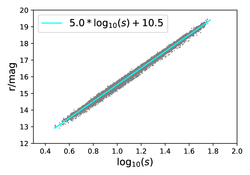
Figure 1: The correlation between $r$-band magnitude and distance for RR-Lyrae stars. The cyan line shows the linear fit employed.

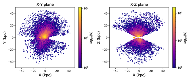
Figure 2: The spatial distribution of the RR-Lyrae sample showing the impact of the selection function.

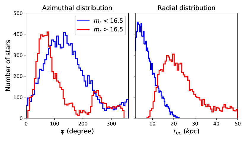
Figure 3: The azimuthal (left) and radial distributions of the stars. The blue and red curves are for stars brighter or fainter than $r=16.5\,$mag, respectively.

3 Observational data

3.1 The RR-Lyrae sample

Our sample derives from the $3\pi$ section of the PanSTARRS1 (PS1) survey (Kaiser et al., 2010). Sesar et al. (2017) used a machine-learning method to identify RR-Lyrae stars in the PanSTARRS1 survey, and determined the purity and completeness of the sample. We set their ‘threshold on score’ to $0.5$ to obtain a sample of RR-Lyrae stars of $0.95$ purity and $0.97$ completeness for the stars at $\sim 18.5\,$mag in the $r$-band, which corresponds to $40\,\mathrm{kpc}$ from the Sun (Sesar et al., 2017). Sesar et al. (2017) conclude that the distances, from the period-luminosity relation, have uncertainties $\sim 3\,$per cent.

We used astrometry from the Gaia mission’s early third data release (Gaia Collaboration, 2021). The typical uncertainties for parallax and proper motion are $0.07\,$mas and $0.07\,\mathrm{mas\,yr}^{-1}$ at $G=17\,$mag and $0.5\,$mas and $0.5\,\mathrm{mas\,yr}^{-1}$ at $G=20\,$mag for 5-parameter solutions (Gaia Collaboration, 2021).

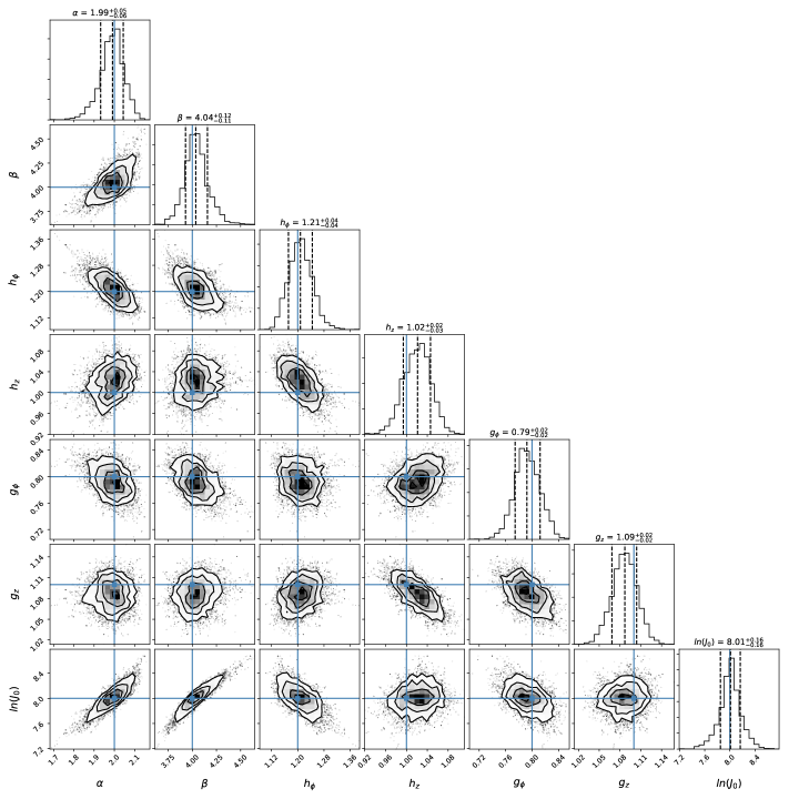
Figure 4: The posterior probability distributions and correlations of the parameters when the DF is fitted to mock data that includes line-of-sight velocities. The dashed lines mark the 1-$\sigma$ uncertainty while the blue lines mark the true value of the parameter.

3.2 Selection function

Sesar et al. (2017) derived the selection function of the RRab stars in PanSTARRS1. It is almost a constant at $\sim 90\,$per cent for $r$-band magnitude $r_{F}<20$, being well fitted by the Fermi-Dirac function

$$S(r_{F})={L\over\exp[k(r_{F}+x_{0})]+1}.$$ (31)

where $L=0.91$ represents the peak value of the selection function, $k=4.1$ is the sharpness and $x_{0}=20.6$ denotes the magnitude at which the completeness drops to $50\,$per cent. Given the almost fixed absolute magnitude of these stars, $r_{F}$ is a function of distance, namely

$$r_{F}=10.5+5\log_{10}(s/\!\,\mathrm{kpc}),$$ (32)

which is based on the linear fit of the r-band apparent magnitude with the distance shown in Figure 1. Substituting equation (32) into equation (31) we obtain the selection function as a function of distance.

In view of the latitude of Hawaii, we consider only stars with $\delta>-29^{\circ}$. To avoid the contamination by the bulge and to avoid stars with large proper-motion errors we restrict the sample to stars with Galactocentric distances $r$ in the range $1.5\,\mathrm{kpc}<r<50\,\mathrm{kpc}$. To avoid the region of high extinction near the Galactic plane and to ensure the sample is dominated by halo stars, we adopt the double cut

$$\frac{|z|}{\sqrt{x^{2}+y^{2}}}>\tan{20^{\circ}},\quad|b|>10^{\circ}.$$ (33)

Given that we are fitting to the data a smooth, axisymmetric model of the stellar halo, we try to exclude stars located in over-dense regions. First, we remove all stars that lie within 10 half-light radii of a globular cluster according to the method in Wegg et al. (2019). We use the Harris (1996) catalogue of globular clusters and adopt $2^{\prime}$ when no half-light radius is listed.

Then we remove stars located in identified halo streams. First, we remove stars at $s>15\,\mathrm{kpc}$ that lie near the plane of the Sgr stream as defined by Majewski et al. (2003). Since stars in the trailing arm of Sgr are spread more widely either side of the Sgr plane than stars in the leading arm, at $x<0$ we delete stars that lie within $15^{\circ}$ of the plane, while at $x>0$ we cut stars that lie within $10^{\circ}$ of the plane. The transformation of equatorial coordinates to Sgr coordinates is taken from Belokurov et al. (2014). We also cut stars that belong to other streams according to Tables 3 and 4 in Yang et al. (2019).

Finally we cross match the RR-Lyrae catalogue with Gaia EDR3 to within a radius of $0.5^{\prime\prime}$ and remove stars without a measurement of proper motion or $\tt{astrometric\_excess\_noise\_sig}>10$. The sample then comprises $19\,154$ RRab stars. The fraction of stars in each of 25 bins in Galactocentric radius that is successfully cross-matched to EDR3 is noted and the selection function that will be applied to models is updated by being multiplied by these fractions.

Figure 2 shows the distribution of the final sample, projected onto the Galactic plane in the left panel and onto the meridional $(R,z)$ plane in the right panel. The Sun’s location is marked by an orange dot. Figure 3, shows the azimuthal and radial distribution of the bright ($r<16.5$ blue curves) and faint stars in the sample. Naturally very few faint stars appear within $10\,\mathrm{kpc}$ of the Galactic centre.

Table 1: Summary of all tests. The second and third rows give the means and 1-$\sigma$ uncertainties of the posterior distributions from a single catalogue. The fourth and fifth rows show the means and standard deviations of the means that were extracted from ten different realisations of the same DF. The units of $J_{0}$ anr $\!\,\mathrm{kpc}\,\mathrm{km\,s}^{-1}$.

		$\alpha$	$\beta$	$h_{\phi}$	$h_{z}$	$g_{\phi}$	$g_{z}$	$\ln{J_{0}}$
	Input Value	2.0	4.0	1.2	1.0	0.8	1.1	8.0
1 catalogue	6D results	$1.99^{+0.05}_{-0.06}$	$4.04^{+0.12}_{-0.11}$	$1.21^{+0.04}_{-0.04}$	$1.02^{+0.02}_{-0.03}$	$0.79^{+0.02}_{-0.02}$	$1.09^{+0.02}_{-0.02}$	$8.01^{+0.16}_{-0.16}$
	5D results	$2.00^{+0.06}_{-0.07}$	$4.14^{+0.24}_{-0.17}$	$1.22^{+0.05}_{-0.05}$	$1.02^{+0.03}_{-0.03}$	$0.78^{+0.03}_{-0.03}$	$1.08^{+0.02}_{-0.02}$	$8.11^{+0.25}_{-0.25}$
10 catalogues	6D results	$2.04\pm 0.05$	$4.24\pm 0.21$	$1.19\pm 0.03$	$1.00\pm 0.02$	$0.78\pm 0.02$	$1.11\pm 0.02$	$8.27\pm 0.21$
	5D results	$2.06\pm 0.07$	$4.40\pm 0.32$	$1.19\pm 0.04$	$1.01\pm 0.02$	$0.76\pm 0.03$	$1.09\pm 0.02$	$8.37\pm 0.32$

4 Tests on mock data

We tested our ability to recover the DF of the RR-Lyrae stars from realistic data as follows. We generated ten sets of mock data by instructing AGAMA to randomly sample a population of RR-Lyrae stars with a known DF – the top row of Table 1 gives the parameters of this DF. The astropy package (Price-Whelan et al., 2018) was used to convert the Cartesian coordinates $({\bf x},{\bf v})$ produced by AGAMA to observational variables ${\bf u}=(\alpha,\delta,s,\mu_{\alpha},\mu_{\delta},v_{\parallel})$ . Each mock star was then included in, or excluded from, the mock catalogue by applying the selection function described in Section 3.2. Finally, the data were scattered by observational errors appropriate to the star’s apparent magnitude. The ten resulting mock catalogues, each with $\sim 20\,000$ stars like the real catalogue, were analysed in two ways: (i) using all six phase-space coordinates ${\bf u}$, and (ii) using only the five astrometric coordinates to mimic the actual case in which spectra are not available.

We used SLSQP method of scipy (Virtanen et al., 2020) to locate a minimum of minus the log-likelihood, and started the MCMC search from this DF. We searched with the emcee package (Foreman-Mackey et al., 2013), with 35 walkers for each parameter and 500 steps in total. The first 50 steps were considered burn-in and do not contribute to the statistics we present.

4.1 Mock catalogue with full 6-D information

Fig. 4 gives results from a single mock catalogue when using the values for $v_{\parallel}$. Each panel shows the marginalized posterior probability distribution of a parameter. The parameter’s true value is where the blue lines intersect. The central dashed line in each one-dimensional histogram marks the median of the distribution, and 68 percent of the probability is contained between it and the dashed lines on either side, at the 16th and 84th percentiles. These lines show that the MCMC exploration is estimating the parameters within the expected uncertainties and with no evidence of bias. The second row of Table 1 summarises the results shown in Fig. 4.

The only strong correlations are between the break action $J_{0}$ and the inner and outer slope parameters $\alpha$ and $\beta$. The existence of this correlation is entirely natural, and it gives rise to the weaker correlation between $\alpha$ and $\beta$ shown in the top left 2-d histogram.

The coefficients $h_{i}$ and $g_{i}$ of the actions, which establish the velocity ellipsoid, are recovered with good precision. The slope $\alpha$ of the inner halo is also recovered well, while the slope $\beta$ of the outer halo, and the break action $J_{0}$ are less precisely recovered. This is to be expected because the stars in the outer halo have relatively large errors in velocity.

4.2 Mock catalogue without line-of-sight velocities

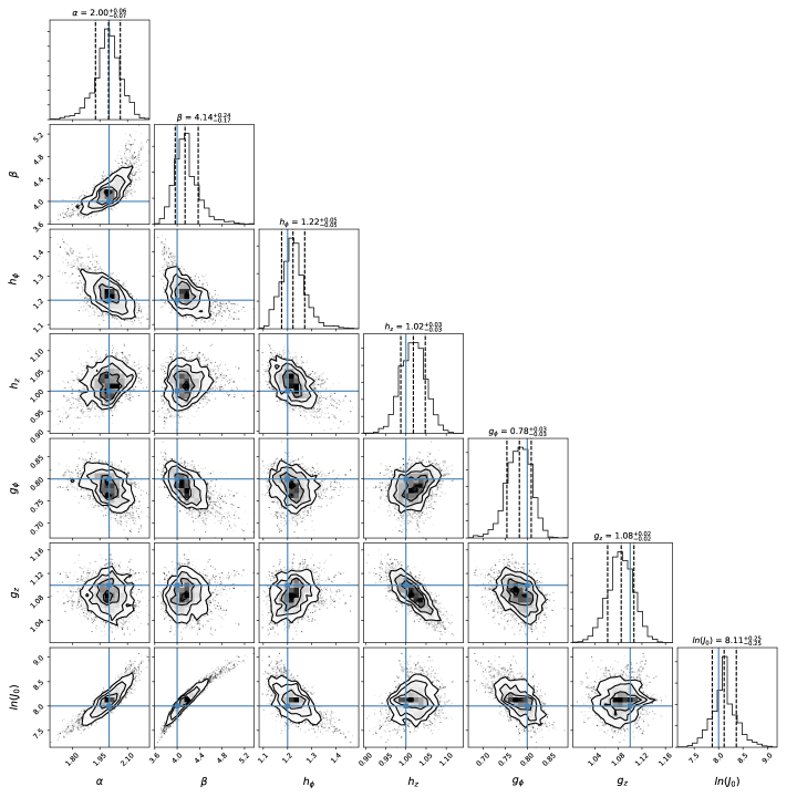
Figure 16: The posterior probability distribution of the each parameter of the mock data without $v_{los}$. The dashed lines mark represent the 1-$\sigma$ uncertainties and the cross points are the input values for the model.

Fig. 16 is the analogue of Fig. 4 for the case in which line-of-sight velocities are not available, and the third row of Table 1 gives the means and standard deviations of its distributions. We see that deleting the line-of-sight velocities introduces no new correlations between the parameters and has rather a small effect on the precision with which the parameters of the DF can be recovered. One might say that the line-of-sight velocities are almost redundant, a conclusion that parallels a result of McMillan & Binney (2012).

4.3 Sanity check

The results presented above involve the analysis of a single mock catalogue, with and without the availability of line-of-sight velocities. In these tests, both observational error and limited sample size contribute to the breadth of the a posterior probability distributions shown in Figs. 4 and 16, which in Table 1 are reduced to means and standard deviations. However, the mean values of these probability distributions are liable to be shifted one way or the other by the peculiarities of the particular realisation of the DF that was analysed. We now investigate the extent of such shifts by examining the scatter in the mean values obtained from ten different catalogues, each a different realisation of the same DF.

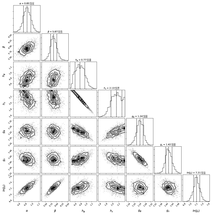
Figure 5: As Fig. 4 but after fitting to the data for real rather than mock RR-Lyrae stars.

Table 2: Means and 1-$\sigma$ uncertainties of parameters fitted to the data for real RR-Lyrae stars.

	$\alpha$	$\beta$	$h_{\phi}$	$h_{z}$	$g_{\phi}$	$g_{z}$	$\ln{J_{0}}$
Fitted Values	$0.85^{+0.12}_{-0.11}$	$5.87^{+0.15}_{-0.13}$	$0.77^{+0.18}_{-0.18}$	$2.13^{+0.18}_{-0.17}$	$1.24^{+0.02}_{-0.02}$	$1.42^{+0.02}_{-0.02}$	$7.21^{+0.11}_{-0.10}$

The bottom two rows of Table 1 list from 6d and 5d analysis, these means-of-means and standard deviations. The standard deviations for parameters other than $J_{0}$ and $\beta$ agree well with the 1-$\sigma$ uncertainties derived from a single catalogue. The means of the correlated parameters $J_{0}$ and $\beta$ both increase in line with the correlation found between them, and the standard deviations of $\beta$, and to a lesser extent $J_{0}$, exceed the 1-$\sigma$ uncertainties from a single catalogue. Overall the ten-catalogue experiment confirms the reliability of statistics extracted from a single catalogue.

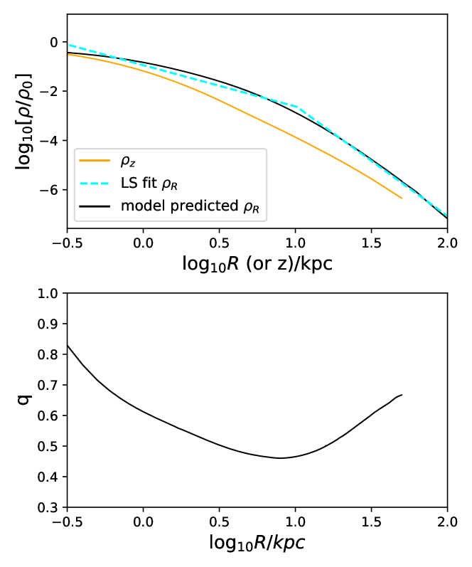
Figure 6: The density distribution predicted by the best-fitting DF. Top: density along the major (black) and minor (orange) axes. The blue lines show a double-power-law fit to the major-axis profile. Bottom: the resulting axis ratio.

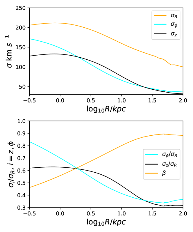
Figure 7: Velocity dispersions along the major axis of the best-fitting model. The lower panel shows the ratios $\sigma_{\phi}/\sigma_{R}$ and $\sigma_{z}/\sigma_{R}$ along the major axis.

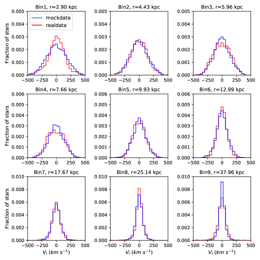
Figure 8: Distributions of $V_{\ell}$ for real RR-Lyrae stars (red histograms) and mock stars drawn from the best-fitting DF. The radius marked in each bin is the median Galactocentric radius of the mock stars in that bin.

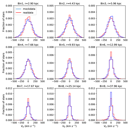
Figure 9: As Fig. 8 but for $V_{b}$.

5 DF parameters from real RR-Lyrae stars

We now apply the method for missing $v_{\parallel}$ to the real RRab catalogue from PanSTARRS and Gaia EDR3. Fig. 5 shows the distributions and correlations of the parameters from the MCMC search. Table 2 shows the means and standard deviations of these distributions.

The principal difference between Fig. 5 and the corresponding figures from the tests is the appearance of a tight correlation between the anisotropy parameters $h_{\phi}$ and $h_{z}$, which are subject to the constraint $h_{z}+h_{\phi}<3$ so that $h$ is non-zero, and the DF is finite, away from the origin of action space. In the tests, the underlying DF is not strongly anisotropic and the constraint plays no role. The DF of the RR-Lyrae stars is well known to be strongly radially biased, and the constraint $h_{\phi}+h_{z}<3$ forces the probable values of the parameters to lie close to the line $h_{\phi}+h_{z}=3$ along which the DF is almost independent of $J_{r}$. Several other studies of halo populations using Gaia DR2 data have concluded that the inner stellar halo is strongly radially biased (Belokurov et al., 2018; Wegg et al., 2019; Bird et al., 2019).

Table 2 indicates that for the RR-Lyrae stars $h_{z}>h_{\phi}$, which implies that the RR-Lyrae population is flattened. Several previous studies have reached this conclusion for sub-populations of the stellar halo (Carollo et al., 2010; Sesar et al., 2011; Das & Binney, 2016; Hernitschek et al., 2018; Wegg et al., 2019).

The values $g_{\phi}=1.24$, $g_{z}=1.42$ and thus $g_{r}=0.34$ derived for the outer halo indicate that the latter is also flattened but not so strongly radially biased as the inner halo. Previous studies of the stellar halo have concluded that its flattening and radial bias decrease with radius (Pila-Díez et al., 2015; Xue et al., 2015; Bird et al., 2019; Wegg et al., 2019; Bird et al., 2020).

The uncertainties in the parameters that define the inner halo are larger than we encountered with the mock catalogues, while similar uncertainties are found in the break action and the parameters that define the outer halo.

5.1 Spatial structure of the population

The upper panel of Fig. 6 shows the density profiles of the RR-Lyrae population in the plane (black curve) and along the symmetry axis (orange curve). The flattening of the model is evident from the fact that the orange curve lies well below the black curve. The cyan dashed lines in this plot show a least-squares fit to the in-plane density profile with two power laws:

$$\rho(r)=\rho_{0}\times\begin{cases}(r_{\rm b}/r)^{\alpha_{\rm i}}&r<r_{\rm b},\cr(r_{\rm b}/r)^{\alpha_{\rm o}}&r>r_{\rm b}.\end{cases}$$ (34)

The break radius $r_{\rm b}$ is encoded in the DF by the break action $J_{0}$, while the inner and outer density slopes $\alpha_{\rm in}$ and $\alpha_{\rm o}$ are encoded in the DF by $\alpha$ and $\beta$. Their best-fit values are $r_{\rm b}=10.2\,\mathrm{kpc},\,\alpha_{\rm i}=1.7,\alpha_{\rm o}=4.5$. A straight line provides a good fit to the model density profile at $R>10\,\mathrm{kpc}$, but no straight line could provide a good fit to the profile at smaller radii. The significant curvature of the density profile inside the break radius reflects the complexity of the potential in this region, where bulge, disc and dark halo all contribute significantly – Posti et al. (2015) showed that the DF we are fitting to the RR-Lyrae stars generates a self-consistent model that is well fitted by a double power law in radius, but our RR-Lyrae model sits in an externally generated potential.

The break radius $r_{\rm b}\simeq 10\,\mathrm{kpc}$ derived above is only half that derived for the stellar halo in other studies (Sesar et al., 2011; Xue et al., 2015; Hernitschek et al., 2018). We defer discussion of this issue to Section 8.

The outer slope in our model, $\alpha_{\rm o}=4.5$, is comparable to the values estimated for other halo populations (Sesar et al., 2011; Xue et al., 2015; Hernitschek et al., 2018). This parameter is vulnerable to the use of an erroneous selection function.

The lower panel of Fig. 6 shows the axis ratio $q$ of isodensity surfaces as a function of semi-major axis length $R$. The population is most flattened around the solar radius because it is there that the disc’s contribution to the overall potential is largest; at smaller and larger radii the bulge and the dark halo dominate.

The upper panel of Fig. 7 shows how the velocity dispersions vary with radius $R$ along the major axis, and the lower panel shows the axis ratios of the velocity ellipsoid. Even though $h_{\phi}+h_{z}$ lies near its upper bound of 3, while $g_{\phi}+g_{z}$ is significantly smaller, the (strong) radial bias is outwards increasing. At $R\la 1\,\mathrm{kpc}$, $\sigma_{\phi}$ tends to $\sigma_{R}$, as it must in any plausible axisymmetric model (Binney & Vasiliev in preparation), but at all radii for which we have observational data, both axis ratios are declining with increasing $R$ from $\sim 0.6$ to $\sim 0.3$. These results are consistent with the findings of Wegg et al. (2019). In the lower panel of Fig. 7, the orange solid line shows the anisotropy parameter $\beta=1-{\textstyle{1\over 2}}(\sigma^{2}_{\theta}+\sigma^{2}_{\phi})/\sigma^{2}_{r}$, which is as large as $\sim 0.9$ beyond $30\,\mathrm{kpc}$ from the Galactic centre. This is consistent with recent studies of the stellar halo (Bird et al., 2019; Lancaster et al., 2019; Bird et al., 2020).

6 Quality control

A best-fit model has significance only to the extent that it provides a convincing fit to the data – if a decent approximation to the true DF can be obtained for no values of its parameters, the fitted DF is unlikely to be able to predict the data even for the best-fit parameters. Hence we now ask whether the best-fit DF successfully accounts for the statistics of the data by comparing the observational catalogue with a mock catalogue constructed by sampling the best-fit DF.

Figs. 8 and 9 compare real (red) and mock (blue) distributions of $V_{\ell}$ and $V_{b}$, respectively. From top left to bottom right the Galactocentric distance of the stars increases from $r>2.9\,\mathrm{kpc}$ to $r<39\,\mathrm{kpc}$. The mock distributions were obtained in a two-step process. The DF was sampled to produce true values of the observables for the same number of stars as there are in real catalogue. The mock stars were then binned in Galactocentric radius $r$ and the effect of observational errors was simulated by smoothing as follows.

First the distributions of the uncertainties in $\mu_{\alpha}$ and $\mu_{\delta}$ for stars in each bin were plotted and appropriate dispersions chosen. Then the probability $P_{ij}$ that a star is scattered by an observational error $\epsilon_{j}$ from the true value $x_{j}$ of an observable into a bin that has boundaries $X_{i-1}<X_{i}$ is

$$P_{i}(x_{j})=\int_{X_{i-1}}^{X_{i}}\frac{{\rm d}x}{\sqrt{2\pi}\epsilon_{j}}\mathrm{e}^{-{(x_{j}-x)^{2}}/{2\epsilon_{j}^{2}}}.$$ (35)

If the true number density of stars is $F(x)$, then the number that will be found in the $i$th bin is

$$N_{i}=\int_{-\infty}^{\infty}{\rm d}x\,P_{i}(x)F(x)$$ (36)

In the approximation that the $F(x)$ is constant across the width of each bin, we have

$$N_{i}\simeq\sum_{j}{n_{j}\over X_{j}-X_{j-1}}\int_{X_{j-1}}^{X_{j}}{\rm d}x\,P_{i}(x)\simeq\sum_{j}n_{j}P_{i}(\overline{x}_{j}),$$ (37)

where $n_{j}=F(\overline{x}_{j})(X_{j}-X_{j-1})$ with $\overline{x}_{j}=\frac{1}{2}(X_{j-1}+X_{j})$ is the number expected in the $j$th bin in the absence of errors.

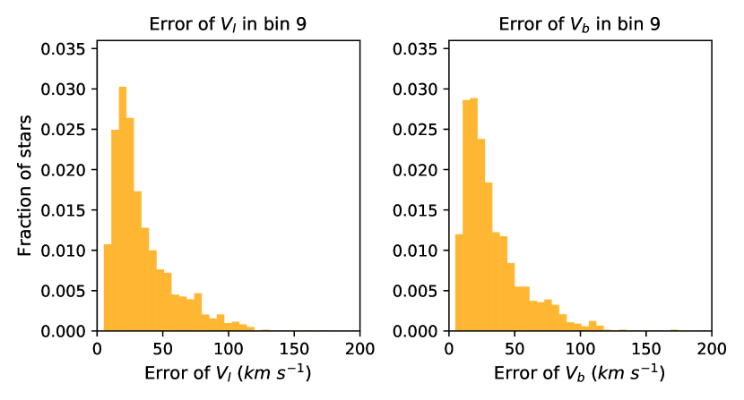
Figure 10: The errors of $V_{\ell}$ (left) and $V_{b}$ for real stars in the bin furthest from the Galactic centre.

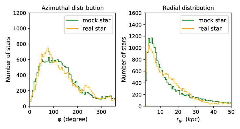
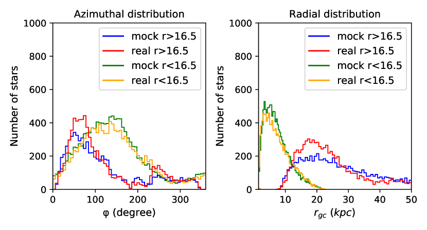
Figure 11: Distributions of stars in Galactocentric azimuth $\phi$ (left column) and radius $r$ (right column). Top row: all real stars (orange) and mock stars (blue) when using the standard selection function. Bottom row: the same catalogues split into brighter ($r<16.5$ orange/blue) and fainter (red/blue) stars.

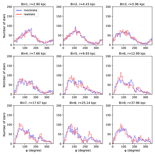
Figure 12: The distribution of $\phi$ for both real RR-Lyrae stars (red histogram) and mock stars drawn from the best-fitting DF. The bins are the same as Figs. 8 and 9.

In Figs. 8 and 9 the observed (red) and predicted (blue) histograms agree quite well at most radii. Both the observed and the mock distributions become narrower as one proceeds to larger radii. This trend reflects the marked falls in the velocity dispersions shown in the upper panel of Fig. 7. With the possible exception of the top left panel of Fig. 8, the red histograms show no evidence of being skew, as they would be if the RR-Lyrae population were systematically rotating. In the top left panel of Fig. 8, for $r\sim 2.9\,\mathrm{kpc}$, there is a hint of skewness, consistent with the finding of Wegg et al. (2019) of rotation at $r<4\,\mathrm{kpc}$. Since we have chosen to use a DF that is even in $J_{\phi}$, the blue histograms should be symmetric to within Poisson noise. However, the skewness of the red histogram is not alone responsible for the disagreement between the red and blue histograms in the top left panel of Fig. 8: the main problem is that the mock distribution is too broad. The corresponding panel of Fig. 9 shows a similar, but weaker, conflict. These conflicts may signal a problem with the functional form of the DF at small $|{\bf J}|$.

In Figs. 8 and 9, the bottom-right panels for the stars furthest from the Galactic centre display the opposite effect: the red histograms are now broader than the blue ones. From left to right along the bottom rows of both figures, the blue histograms become steadily narrower in line with the fall in $\sigma$ with increasing $r$. In the first two panels, the red histograms follow suit, but in the third panels the red histograms broaden. Is this phenomenon real or a reflection of problems with the data? In the former case, we should modify the DF at large $|{\bf J}|$. On the other hand, the data for these most distant stars $\left<r\right>\simeq 39\,\mathrm{kpc}$ are subject to large uncertainties, as is illustrated by the broad and highly non-Gaussian distribution of uncertainties in $V_{\ell}$ and $V_{b}$ plotted in Fig. 10. Moreover, stars with the most over-estimated distances will accumulate in this bin alongside inflated values of $V_{\ell}$ and $V_{b}$.

The upper row of Fig. 11 compares the observed (orange) and mock (blue) distributions in Galactocentric azimuth $\phi$ (left panel) and radius $r$. Systematic differences in the distributions are evident. The lower row of Fig. 11 probes the origin of these differences by showing the azimuthal and radial distributions separately for stars brighter/fainter than magnitude $r=16.5$. We see that the mock and observed histograms for the brighter stars agree well and the discrepancies lie with the distributions of faint stars: in the lower right panel of Fig. 11, the mock sample (blue) contains too few faint stars at $r_{\rm gc}\sim 20\,\mathrm{kpc}$ and a slight excess at large radii. This issue cannot be resolved by simply changing the model’s density profile because the yellow and green curves for bright stars agree well at $r\sim 20\,\mathrm{kpc}$: at this radius the model works well in the anticentre direction but at most distant locations it predicts too few stars. The lower left panel shows that the deficiency is concentrated at longitudes $\ell=80$ and 240 degrees. Two explanations are in principal viable: the stellar halo, unlike the model, is not axisymmetric, having enhanced density at $\ell\sim 80$ and 260 degrees, or the (very much non-axisymmetric) selection function that we have applied to the model is incorrect and culls too many stars at the given longitudes.

6.1 Overdensities

Fig. 12 compares the observed and mock distributions in Galactocentric azimuth $\phi$ when the sample is divided into bins by Galactocentric radius as in Figs. 8 and 9. The agreement is particularly good out to the solar radius, but from the fifth bin ($r\sim 10\,\mathrm{kpc}$) onwards the red histograms for real stars show more structure than the mock blue histograms. Is this additional structure caused by stellar streams that we have not eliminated from the data? Smooth structure at $r<R_{0}$ and sharp local peaks in density further out is exactly the pattern that streams would be expected to generate.

It is interesting that the blue histograms do have local peaks that correspond to peaks in the red histograms (e.g., at $\phi\sim 180^{\circ}$ in the central panel and at $\phi\sim 230^{\circ}$ in the leftmost panels of the bottom row). The conflict between the histograms is just that these features have larger amplitude in the red than in the blue histograms. Streams contribute to the blue histograms in that our selection function, which culls mock stars sampled from the DF, is designed to exclude streams. Since our selection function includes some but not all streams, it is to be expected that the mock and true histograms show similar structure, with more structure in the true histograms.

Streams other than Sgr were cut from the data using tables in Yang et al. (2019), which were compiled from LAMOST spectroscopic data. LAMOST operates at rather bright magnitudes and has a more complex selection function than the photometric surveys PanSTARRS and Gaia. Consequently, our data probably do contains streams that were missed by Yang et al. (2019), particularly at faint magnitudes $r\sim 18.5$.

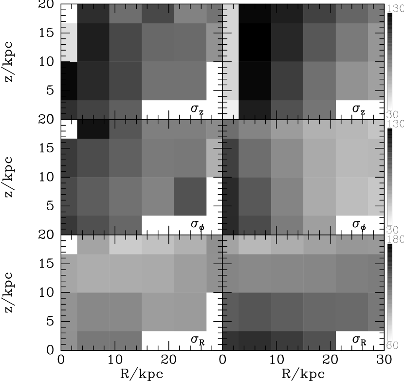
Figure 13: Left column: the principal velocity dispersions (in spherical coordinates) of the observed BHB stars when binned in $(R,|z|)$. Right column: the dispersions predicted by our model of the RR-Lyrae population.

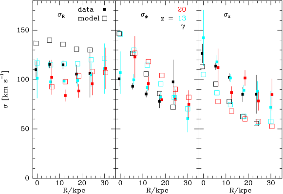
Figure 14: Velocity dispersions of the BHB population along three lines of constant distance from the plane, as functions of cylindrical radius $R$. The bins are those shown in Fig. 13 less the bottom row in each panel. Error bars are only shown for the data – there are 20 times as many mock stars as real ones, so the uncertainties of the model dispersions are smaller by a factor $\sim 4.5$.

7 Does the model fit BHB stars?

RR-Lyrae stars might be expected to trace the metal-poor halo, and in this section we compare our model of the RR-Lyrae population with the sample of nearly 5000 BHB stars from Xue et al. (2011). Accurate spectrophotometric distances and line-of-sight velocities are available for BHB stars, and we complement these with proper motions from Gaia EDR3. We exclude stars that appear unbound or lie close to a globular cluster or within the Sagittarius stream. We further exclude stars with very uncertain velocities by imposing the criterion

$$\sqrt{\epsilon^{2}_{v_{x}}+\epsilon^{2}_{v_{y}}+\epsilon^{2}_{v_{z}}}<50\,\mathrm{km\,s}^{-1}.$$ (38)

After these cuts, 2231 BHB stars remain in the sample.

The selection function involved in the identification of BHB stars by Xue et al. (2011) is complex and poorly determined, so we will not concern ourselves with the spatial distribution of the BHB stars. Fortunately, the selection function should be blind as regards velocity, so we ask to what extent our model predicts the velocity distribution of the BHB stars.

At the location of each BHB star, we instructed AGAMA to sample the velocity distribution in our model and thus produce 20 mock BHB stars at that location. Then we binned both the real and mock BHB stars in a grid in the $Rz$-plane and compared the $Rz\phi$ velocity dispersions of the two samples in cells that contain a useful number of real BHB stars.

Figs 13 and 14 show the results. The top row in Fig. 13 and the extreme right panel of Fig. 14 show that the model predicts $\sigma_{z}$ quite well. The middle panels of both figures indicate that at Galactocentric radii similar to $R_{0}$ the model values for $\sigma_{\phi}$ are on the high side, while the bottom panels of Fig. 13 and the extreme left panel of Fig. 14 indicate that near the plane the model values of $\sigma_{R}$ are too large.

The stellar halo is now recognised to contain sub-populations. In particular, recent work has identified a sub-population, the ‘Gaia sausage’ of relatively metal-rich stars on highly eccentric orbits that is speculated to have formed during an early major merger (Helmi et al., 2018; Belokurov et al., 2018; Lancaster et al., 2019; Iorio & Belokurov, 2021; Wu et al., 2021). In the likely event that the proportions of sausage stars in the RR-Lyrae and BHB populations are different, one would expect RR-Lyrae and BHB kinematics to differ. Hence the differences between model and data in Figs. 13 and 14 do not necessarily reflect weaknesses of the model. When spectra are available for a significant fraction of the RR-lyrae stars, it is likely that a more complex model of the RR-Lyrae population will be required in chemically identified sub-populations have distinct kinematics.

8 Prior work

8.1 Wegg et al. 2019

Wegg et al. (2019, hereafter W19) modelled a very similar data set for $15\,813$ RR-Lyrae stars at $r<20\,\mathrm{kpc}$ in a different way: they fitted a parametrised model

$$\nu(r,\theta)=r^{-\alpha}\Big{(}\sin^{2}\theta+{\cos^{2}\theta\over q^{2}}\Big{)}^{-\alpha/2}$$ (39)

to the stars’ spatial distribution and assumed that at each location the density of stars in velocity space is a function $F(Q)$ of

$$Q({\bf v})\equiv{\textstyle{1\over 2}}({\bf v}-\overline{{\bf v}})^{T}\cdot{\bf K}\cdot({\bf v}-\overline{{\bf v}}),$$ (40)

where $\overline{\bf v}=v_{\phi}{\bf e}_{\phi}$ is the mean azimuthal streaming velocity and

$${\bf K}\equiv\left(\begin{matrix}\sigma_{rr}^{-2}&\sigma_{r\theta}^{-2}&0\cr\sigma_{r\theta}^{-2}&\sigma_{\theta\theta}^{-2}&0\cr 0&0&\sigma_{\phi\phi}^{-2}\end{matrix}\right).$$ (41)

The function $F$, ${\bf v}_{\phi}$ and the four independent elements of ${\bf K}$ were determined by distributing the stars over $n_{r}\times n_{\theta}$ bins in the meridional plane. This procedure has the merit that it does not require prior specification of the Galaxy’s potential. Indeed, W19 were able to constrain the Galaxy’s gravitational field by applying the Jeans equations to an estimate of the stellar stress field $(\nu{\mathchoice{\hbox{{\gkvecten\char 27\relax}}}{\hbox{{\gkvecten\char 27\relax}}}{\hbox{{\gkvecseven\char 27\relax}}}{\hbox{{\gkvecseven\char 27\relax}}}}^{2})({\bf x})$ that they obtained from equation (39) and their grid of values for ${\mathchoice{\hbox{{\gkvecten\char 27\relax}}}{\hbox{{\gkvecten\char 27\relax}}}{\hbox{{\gkvecseven\char 27\relax}}}{\hbox{{\gkvecseven\char 27\relax}}}}^{2}$.

W19 adopted $n_{r}=8$ and $n_{\theta}=5$ and hence invoked $2+5n_{r}n_{\theta}=202$ free parameters. It is not a given that the density in velocity space is a function of the quadratic form $Q$ and the imbalance in the distribution of parameters between structure in real space (2 parameters) and velocity space (200 parameters) is surely not ideal. Clearly W19 could not show a figure analogous to Figs. 4, 5 and 16 for 202 parameters, but they do say that many of their parameters are highly correlated.

In formulating a model, the goal should be to obtain a good fit to the data using the smallest number of least correlated parameters. From this perspective our model with seven parameters and only one significant correlation in the tests is at an advantage to that of W19. Unfortunately, when we applied the model to the real data a second, even stronger correlation appeared, that between $h_{\phi}$ and $h_{z}$. This correlation points to a fundamental weakness in the procedure for introducing velocity anisotropy that was proposed by Binney (2014). This issue will be addressed in forthcoming paper. Moreover, our DF is an even function of $J_{\phi}$ and thus excludes the possibility of systematic rotation, for which W19 found evidence at $r\la 4\,\mathrm{kpc}$. In future work we will increase our parameter count by adding a part odd in $J_{\phi}$ to the DF. Even after a modest increase in parameter count, the present method will still involve an order-of-magnitude fewer parameters that that of W19.

8.2 Pros and cons of modelling the DF

The $f({\bf J})$ modelling technique holds down the number of parameters required to fit rich data by exploiting Jeans’ theorem, which connects real space to velocity space. The price one pays for this advantage is that to predict observables one requires both a DF and a potential $\Phi({\bf x})$. When modelling the entire Galaxy, $\Phi$ can be derived from the DF by the self-consistency principle (Binney, 2014; Binney & Piffl, 2015; Cole & Binney, 2017). When using a tracer population, the $f({\bf J})$ approach requires one to investigate how well one’s form for $f({\bf J})$ can fit the data when different potentials are used. An exploration of this process using mock data by McMillan & Binney (2013) showed that care is needed to keep Poisson noise under control. We hope shortly to constrain our Galaxy’s potential in this way using the present RR-Lyrae data and improved forms of the DF. We expect to be able to break the existing degeneracy between the dark halo and the disc in which a more flattened dark halo and less massive disc generates similar near-plane kinematics to a less flattened dark halo and more massive disc (Binney & Piffl, 2015).

The real-space approach of W19 allows for a more direct assault on the constraint of $\Phi$ but it is still fraught with difficulty because the Jeans equations require derivatives of the stress $\nu{\mathchoice{\hbox{{\gkvecten\char 27\relax}}}{\hbox{{\gkvecten\char 27\relax}}}{\hbox{{\gkvecseven\char 27\relax}}}{\hbox{{\gkvecseven\char 27\relax}}}}^{2}$, which can only be obtained by binning stars on a grid. Refining the grid increases both the parameter count and the amplitude of Poisson noise. When a coarse grid is used the inferred potential depends significantly on the interpolation scheme used to extract derivatives. Moreover, the pressure gradient that betrays the gravitational field depends more strongly on the density $\nu$ than on the velocity dispersion tensor ${\mathchoice{\hbox{{\gkvecten\char 27\relax}}}{\hbox{{\gkvecten\char 27\relax}}}{\hbox{{\gkvecseven\char 27\relax}}}{\hbox{{\gkvecseven\char 27\relax}}}}^{2}$, so assigning two parameters to the former and 200 parameters to the latter cannot be optimal.

As the density and flattening profiles of our model plotted in Fig. 6 illustrate, a DF $f({\bf J})$ which is a simple function of the actions can generate a complex three-dimensional structure because the latter reflects the structure of the potential in addition to that of the DF. Whether this feature of $f({\bf J})$ modelling is a strength or a weakness hinges on whether real components have simpler DFs than density profiles. We suspect that they do, but this view is open to challenge.

8.3 Break radius

The density profile (39) adopted by W19 is a single power law, and they derived slope $\alpha=2.6$. Similar results with stellar haloes modelled by a single power law $\rho\propto r^{-\alpha}$ were obtained by Iorio et al. (2018) and Mateu & Vivas (2018), who found $\alpha=2.96$ and 2.78, respectively. A simple power inevitably predicts divergent mass as either $r\to 0$ or $r\to\infty$ (or both when $\alpha=3$). Hence most authors have fitted broken power laws to components of the stellar halo. Our break radius $r_{\rm b}\sim 10\,\mathrm{kpc}$ is significantly smaller than previously reported values.

Hernitschek et al. (2018) derived a break radius $38.7\,\mathrm{kpc}$ but this is the radius of a transition from a steeper slope ($\alpha=4.97$) at $r<r_{\rm b}$ to a shallower slope ($\alpha=3.93$) at $r>r_{\rm b}$. Clearly, the steep slope $\alpha=4.97$ cannot continue to the origin. We do not feel able to constrain the density profile at $r>39\,\mathrm{kpc}$, and in the range $10\la r/\!\,\mathrm{kpc}\la 40$ our slope $4.5$ is broadly consistent with the result of Hernitschek et al. (2018).

Several recent studies derive radii at which the slope of a halo population steepens outwards. Watkins et al. (2009) fitted a double power-law to RR-Lyrae stars in SDSS, and found that at $r_{\rm b}=25\,\mathrm{kpc}$ the index steepens from $2.5$ to $4.5$. Sesar et al. (2011) give a break radius $r_{\rm b}=27.8\,\mathrm{kpc}$ at which the slope of the RR-Lyrae population increases from $\alpha=2.62$ to $3.8$. Sesar et al. (2013) found that at $r_{\rm b}=18\,\mathrm{kpc}$ the logarithmic slope steepens from $1.6$ to $3.4$. From a sample of K giants Xue et al. (2015) found that at $r_{\rm b}=18\,\mathrm{kpc}$ $\alpha$ increases from $2.1$ to $3.8$.

Fig. 15 compares our density profile with those of Watkins et al. (2009), Sesar et al. (2011), Sesar et al. (2013), and Xue et al. (2015). The densities predicted by these curves disagree with one another only slightly less than they do with the densities predicted by our model, which are shown by the full black curve. Thus break radii that differ by nearly a factor 3 do not necessarily imply significantly differing observationally testable predictions.

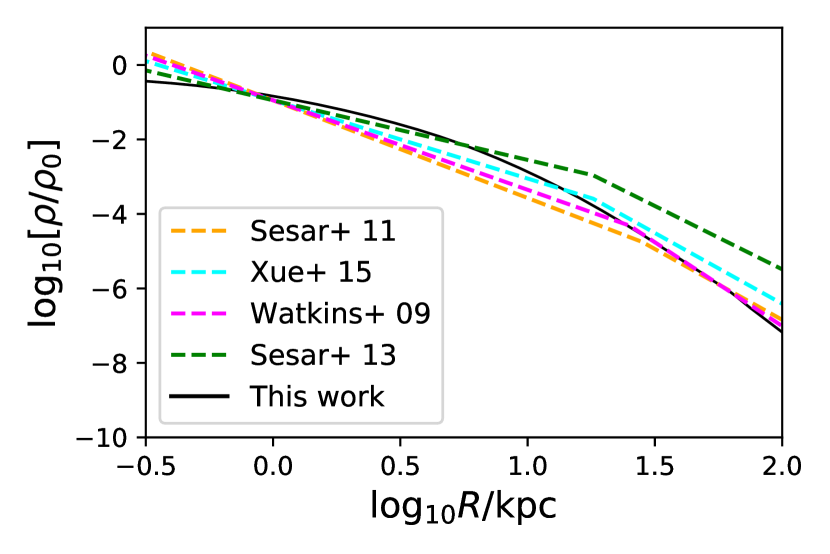
Figure 15: Comparisons between our best-fit model and four prior works Watkins et al. (2009), Sesar et al. (2011), Sesar et al. (2013), and Xue et al. (2015).

9 Conclusions

We have fitted an $f({\bf J})$ model to the Galaxy’s population of RR-Lyrae stars using a sample of $\sim 20\,000$ stars for which precise distances are available but line-of-sight velocities are lacking. This exercise is of interest both for the light it casts on the structure of our Galaxy’s stellar halo and as an exploration of what can be achieved in the absence of line-of-sight velocities. Learning to exploit such data is important given that line-of-sight velocities are unlikely ever to be available for the vast majority of the $\sim 1.3$ billion stars for which Gaia is harvesting astrometry. McMillan & Binney (2012) suggested that one could deal with missing data simply by setting to infinity the error on quantities not measured. While correct in principle, this idea does not work in practice. The procedure developed here for dealing with missing data may prove the most valuable contribution of this paper.

We fit a DF to the data by MCMC exploration of the seven-dimensional space of model parameters. We have tested our code’s ability to infer the parameters of the model with which pseudo data was generated. We did this both for the case in which line-of-sight velocities are available and when they are not. In every case the true parameters lay within the probable region of parameter space identified by the code, and deleting the line-of-sight velocity information enlarged the probable region to a surprisingly small extent. Thus when accurate astrometry is available, line-of-sight velocities are a luxury without which it is straightforward to construct a population’s DF.

In the tests, the only parameters that are significantly correlated are the slopes of the DF at small and large $|{\bf J}|$, and the break action $J_{0}$ that divides their two regimes. A correlation of this type is invariably encountered when fitting a double power-law model to data. With the given sample size and observational errors characteristic of Gaia EDR3, the only parameter that is not tightly constrained is the break action $J_{0}$, which has a 1-$\sigma$ uncertainty $\sim 10$ per cent.

The standard Bayesian technique used here yields posterior probability distributions of parameters that are broadened by both experimental error and Poisson noise. Hence, the means and standard deviations of parameters extracted from a single realisation should agree with the standard deviation obtained from the means of a sequence of different realisations of different models. Table 1 tests this conjecture and confirms it with the possible exception of the correlated parameters $\beta$ and $J_{0}$.

When we apply the code to the real sample of RR-Lyrae stars, there is one material difference: now the parameters $h_{\phi}$ and $h_{z}$ that characterise the velocity ellipsoids and flattening of the inner halo become strongly anti-correlated. In fact the data push them up against the limit $h_{\phi}+h_{z}<3$ that one imposes to ensure that the DF will not diverge at finite $|{\bf J}|$. This result reflects the strong radial bias of the inner halo, a phenomenon that has been interpreted as due to an early merger with the ‘Enceladus’ galaxy (Belokurov et al., 2018). The appearance of a strong correlation between parameters signals the need for improved functional forms for $f({\bf J})$ when fitting strongly anisotropic components. This need will be addressed shortly.

Our model of the RR-Lyrae population is a flattened spheroid in which the density settles to $\rho\sim r^{-4.5}$ at radii $r\ga 10\,\mathrm{kpc}$. At smaller radii the density is not well fitted by a power law although at $r<0.3\,\mathrm{kpc}$, ${\rm d}\ln\rho/{\rm d}\ln r\sim-1.7$. In the equatorial plane $\sigma_{\theta}\ga 0.4\sigma_{r}$, so the model is not exceptionally strongly radially biased, notwithstanding the limiting value of $h_{\phi}+h_{z}$. In the region probed by the data, the ratios $\sigma_{\phi}/\sigma_{r}$ and $\sigma_{\theta}/\sigma_{r}$ fall from $\sim 0.6$ to $\sim 0.3$ consistent with the results of Wegg et al. (2019).

A key issue when fitting a model to high-dimensional data by likelihood maximisation is whether the best-fitting model provides an acceptable fit to the data. Our model provides adequate fits to histograms of the tangential velocities of stars in bins of Galactocentric radius except for stars nearest and furthest from the Galactic centre. These discrepancies may may reflect the very uncertain velocities of these stars. The distributions in both radius and azimuth of bright stars are accurately predicted by the model, but the model predicts too few faint stars at radii $r\sim 20\,\mathrm{kpc}$ at longitudes $\ell\sim 80$ and 240 degrees. Merely changing the model’s radial density profile cannot resolve this issue; the problem could lie with our selection function, or reflect departure of the stellar halo from axisymmetry.

Likely footprints of stellar streams are visible in plots of the azimuthal distributions of stars binned by Galactocentric radius $r$. Inside the solar sphere we don’t expect significant contributions from streams, and indeed at these radii the mock and real catalogues agree nicely. At larger radii the real histograms show more substructure than the mock ones, as would be expected if streams contribute to the data despite our efforts to exclude known streams. The mock histograms have less pronounced local maxima at similar azimuths to the real histograms, perhaps because the mock data were filtered by a selection function designed to mask streams.

We used our model of the RR-Lyrae population to predict the velocity distribution at the locations of BHB stars with measured space velocities. The $z$ velocities are predicted well but too much elongation was predicted in the $v_{R}v_{\phi}$ plane. This problem may reflect real differences between the BHB population and the slightly more metal-rich RR-Lyrae population, or a poor choice for the form of the DF.

This work constitutes a proof of principle: five-dimensional data such as Gaia provides for over a billion stars can be used to build a dynamical model of a stellar component. This opens up two avenues for further work. First improved functional forms of the DF will be fitted to the present sample of RR-Lyrae stars in the potential generated by a series of self-consistent Galaxy models. A prime focus of this work will be on constraining the shape and local density of the dark halo by using the RR-Lyrae stars to probe the potential further from the plane and out to larger radii than stars in Gaia’s RVS sample do.

A second natural application of the approach we have developed here would be use stars not in the RVS catalogue alongside RVS stars in the construction of self-consistent Galaxy models.

DATA AVAILABILITY

The data underlying this article are available in the article and in its online supplementary material.

Appendix A Parameter correlations without $v_{\parallel}$

References

- Bell et al. (2008) Bell E. F., et al., 2008, ApJ, 680, 295
- Belokurov et al. (2014) Belokurov V., et al., 2014, MNRAS, 437, 116
- Belokurov et al. (2018) Belokurov V., Erkal D., Evans N. W., Koposov S. E., Deason A. J., 2018, MNRAS, 478, 611
- Belokurov et al. (2020) Belokurov V., Sanders J. L., Fattahi A., Smith M. C., Deason A. J., Evans N. W., Grand R. J. J., 2020, MNRAS, 494, 3880
- Binney (2014) Binney J., 2014, MNRAS, 440, 787
- Binney & Piffl (2015) Binney J., Piffl T., 2015, MNRAS, 454, 3653
- Binney & Wong (2017) Binney J., Wong L. K., 2017, MNRAS, 467, 2446
- Binney et al. (2014) Binney J., et al., 2014, MNRAS, 439, 1231
- Bird et al. (2019) Bird S. A., Xue X.-X., Liu C., Shen J., Flynn C., Yang C., 2019, AJ, 157, 104
- Bird et al. (2020) Bird S. A., Xue X.-X., Liu C., Shen J., Flynn C., Yang C., 2020, arXiv e-prints, p. arXiv:2005.05980
- Bland-Hawthorn & Gerhard (2016) Bland-Hawthorn J., Gerhard O., 2016, AnnRA&A, 54, 529
- Bovy (2014) Bovy J., 2014, ApJ, 795, 95
- Carollo et al. (2010) Carollo D., et al., 2010, ApJ, 712, 692
- Cole & Binney (2017) Cole D. R., Binney J., 2017, MNRAS, 465, 798
- Das & Binney (2016) Das P., Binney J., 2016, MNRAS, 460, 1725
- Deason et al. (2011) Deason A. J., Belokurov V., Evans N. W., 2011, MNRAS, 416, 2903
- Deason et al. (2019) Deason A. J., Belokurov V., Sanders J. L., 2019, MNRAS, 490, 3426
- Dehnen & Binney (1998) Dehnen W., Binney J., 1998, MNRAS, 294, 429
- Erkal et al. (2016) Erkal D., Belokurov V., Bovy J., Sanders J. L., 2016, MNRAS, 463, 102
- Foreman-Mackey et al. (2013) Foreman-Mackey D., Hogg D. W., Lang D., Goodman J., 2013, PASP, 125, 306
- Gaia Collaboration (2021) Gaia Collaboration 2021, A&A, 649, A1
- Gaia Collaboration et al. (2018) Gaia Collaboration et al., 2018, A&A, 616, A1
- Gibbons et al. (2016) Gibbons S. L. J., Belokurov V., Erkal D., Evans N. W., 2016, MNRAS, 458, L64
- Harris (1996) Harris W. E., 1996, AJ, 112, 1487
- Helmi et al. (2018) Helmi A., Babusiaux C., Koppelman H. H., Massari D., Veljanoski J., Brown A. G. A., 2018, Nat, 563, 85
- Hernitschek et al. (2018) Hernitschek N., et al., 2018, ApJ, 859, 31
- Iorio & Belokurov (2021) Iorio G., Belokurov V., 2021, MNRAS, 502, 5686
- Iorio et al. (2018) Iorio G., Belokurov V., Erkal D., Koposov S. E., Nipoti C., Fraternali F., 2018, MNRAS, 474, 2142
- Jeans (1915) Jeans J. H., 1915, MNRAS, 76, 70
- Kaiser et al. (2010) Kaiser N., et al., 2010, in Proc. SPIE. p. 77330E, doi:10.1117/12.859188
- Koposov et al. (2009) Koposov S. E., Rix H.-W., Hogg D. W., 2009, ApJ, submitted, (arXiv: 0907.1085),
- Koposov et al. (2019) Koposov S. E., et al., 2019, MNRAS, 485, 4726
- Lancaster et al. (2019) Lancaster L., Koposov S. E., Belokurov V., Evans N. W., Deason A. J., 2019, MNRAS, 486, 378
- Majewski et al. (2003) Majewski S. R., Skrutskie M. F., Weinberg M. D., Ostheimer J. C., 2003, ApJ, 599, 1082
- Mateu & Vivas (2018) Mateu C., Vivas A. K., 2018, MNRAS, 479, 211
- McMillan & Binney (2012) McMillan P. J., Binney J., 2012, MNRAS, 419, 2251
- McMillan & Binney (2013) McMillan P. J., Binney J. J., 2013, MNRAS, 433, 1411
- Myeong et al. (2019) Myeong G. C., Vasiliev E., Iorio G., Evans N. W., Belokurov V., 2019, MNRAS, 488, 1235
- Pila-Díez et al. (2015) Pila-Díez B., de Jong J. T. A., Kuijken K., van der Burg R. F. J., Hoekstra H., 2015, A&A, 579, A38
- Posti et al. (2015) Posti L., Binney J., Nipoti C., Ciotti L., 2015, MNRAS, 447, 3060
- Price-Whelan et al. (2018) Price-Whelan A. M., et al., 2018, AJ, 156, 123
- Schönrich (2012) Schönrich R., 2012, MNRAS, 427, 274
- Sesar et al. (2011) Sesar B., Jurić M., Ivezić Ž., 2011, ApJ, 731, 4
- Sesar et al. (2013) Sesar B., et al., 2013, AJ, 146, 21
- Sesar et al. (2017) Sesar B., et al., 2017, AJ, 153, 204
- Vasiliev (2019a) Vasiliev E., 2019a, MNRAS, 482, 1525
- Vasiliev (2019b) Vasiliev E., 2019b, MNRAS, 484, 2832
- Virtanen et al. (2020) Virtanen P., et al., 2020, Nature Methods,
- Watkins et al. (2009) Watkins L. L., et al., 2009, MNRAS, 398, 1757
- Wegg et al. (2019) Wegg C., Gerhard O., Bieth M., 2019, MNRAS, 485, 3296
- Wilkinson & Evans (1999) Wilkinson M. I., Evans N. W., 1999, MNRAS, 310, 645
- Wu et al. (2021) Wu W., Zhao G., Xue X.-X., Bird S. A., Yang C., 2021, arXiv e-prints, p. arXiv:2110.15571
- Xue et al. (2011) Xue X.-X., et al., 2011, ApJ, 738, 79
- Xue et al. (2015) Xue X.-X., Rix H.-W., Ma Z., Morrison H., Bovy J., Sesar B., Janesh W., 2015, ApJ, 809, 144
- Yang et al. (2019) Yang C., et al., 2019, ApJ, 880, 65