Automatic Segmentation of the Optic Nerve Head Region in Optical Coherence Tomography: A Methodological Review

Abstract

The ONH represents the intraocular section of the optic nerve, which is prone to damage by IOP. The advent of OCT has enabled the evaluation of novel ONH parameters, namely the depth and curvature of the LC. Together with the BMO-MRW, these seem to be promising ONH parameters for diagnosis and monitoring of retinal diseases such as glaucoma. Nonetheless, these OCT derived biomarkers are mostly extracted through manual segmentation, which is time-consuming and prone to bias, thus limiting their usability in clinical practice. The automatic segmentation of ONH in OCT scans could further improve the current clinical management of glaucoma and other diseases. This review summarizes the current state-of-the-art in automatic segmentation of the ONH in OCT. PubMed and Scopus were used to perform a systematic review. Additional works from other databases (IEEE, Google Scholar and ARVO IOVS) were also included, resulting in a total of 27 reviewed studies. For each algorithm, the methods, the size and type of dataset used for validation, and the respective results were carefully analyzed. The results show that deep learning-based algorithms provide the highest accuracy, sensitivity and specificity for segmenting the different structures of the ONH including the LC. However, a lack of consensus regarding the definition of segmented regions, extracted parameters and validation approaches has been observed, highlighting the importance and need of standardized methodologies for ONH segmentation.

Keywords: Optical Coherence Tomography, Segmentation, Optic Nerve Head, Lamina Cribrosa

1 Introduction

OCT is an imaging technique that enables noninvasive cross-sectional imaging of tissue using low-coherence interferometry. Among its many applications, one of the most common is the analysis of the human retina where, given its high resolution and three-dimensional nature, OCT can assist in the diagnosis and prognosis of several diseases.

One example of such diseases is glaucoma, which is the main cause of irreversible blindness worldwide, and which has elevated IOP as primary risk factor for its development (Sigal et al., 2005). It starts to manifest through damage to the RGC axons as they exit the eye at the ONH (Tan et al., 2018), and is associated with complex 3D structural modifications in the ONH, such as thinning of the RNFL, changes in the BMO-MRW and in the LC depth, thickness and curvature (Tan et al., 2018; Bekkers et al., 2020; Lee et al., 2017; De Jesus et al., 2020; Jesus et al., 2019). Evidence suggests that the ONH surface depression occurs before the RNFL thinning (Xu et al., 2014), making it more relevant for early diagnosis.

Even though ONH structural changes have been mostly studied in a context of glaucoma diagnosis, they are also representative of non-ophthalmic diseases such as IIH, ON, MS or NMOSD (Yadav et al., 2018), Alzheimer (Cabrera DeBuc et al., 2019; Lemmens et al., 2020), and Parkinson’s disease (Eraslan et al., 2016).

The LC is a mesh-like structure that fills the posterior scleral foramen where unmyelinated RGC axons pass through before exiting the eye (Tan et al., 2018). Up until recently, it has been difficult to study this region of the ONH, given its deep location. The OCT signal is highly attenuated when reaching deeper structures, and the shadow of the blood vessels, which merge at the ONH, can limit the correct identification of the LC and other ONH structures (Yadav et al., 2018). However, it is now possible to overcome some of these problems thanks to advances in imaging technologies such as EDI (Park et al., 2012), SS-OCT (Takusagawa et al., 2019) and adaptive compensation (Mari et al., 2013b).

Given the diagnostic potential of biomarkers extracted from the ONH, and particularly from the LC (Paulo et al., 2021), an accurate segmentation of this region is becoming increasingly important for improving clinical diagnosis and follow-up, and also for contributing to a better understanding of several ophthalmic and non-ophthalmic diseases.

The need for an automatic segmentation arises from the fact that manual segmentation is time consuming, prone to bias, and unsuitable for a clinical environment (Lang et al., 2013) since it requires extensive training and expertise. Even if some commercial OCT devices already have an in-built proprietary segmentation software, they can segment some, but not all, ONH tissues, and they still require frequent manual corrections (Devalla et al., 2020).

The democratization and emergence of OCT as the clinical gold-standard for in vivo structural ophthalmic examinations (Fujimoto and Swanson, 2016) has encouraged the entry of new manufacturers to the market as well. It will soon become practically infeasible to perform manual segmentations for all OCT brands, device models, generations, and applications (Devalla et al., 2020). From this arises the urgent need for device-independent automatic segmentation algorithms.

This review summarizes the current state-of-the-art in automatic segmentation of the ONH in OCT.

2 Methods

A literature search was conducted in MEDLINE (Pubmed) and Scopus bibliographic databases on the 24^th of November 2020. The search query (PubMed) was: (imag* AND processing OR segmentation) AND (optic AND (disc OR disk) OR lamina) AND (optical AND coherence AND tomography) NOT (fundus OR angiography). Additional works which were not found by Pubmed and Scopus, but were cited in the bibliography, and could be found by Google Scholar, IEEE or ARVO bibliographic databases, were also added. Only articles published in English with a detailed description of the method used were considered, and no publication date restriction was added. The exclusion criteria were: (i) no description of a novel segmentation algorithm; (ii) no segmentation of the ONH; (iii) only used en-face images; (iv) review article; (v) case report; (vi) comparative study; (vii) clinical trial; or (viii) not an article (abstracts, book chapters, editorials, and notes).

3 Results

The systematic search led to a total of 565 references after removing the duplicates, which were narrowed down to 31 after title/abstract screening, and finally to 27 after a full-text screening (Figure 1). The 27 included studies provided the description of a fully automatic segmentation of ONH centered OCT B-scans and/or volumes, and described how its performance was evaluated.

All algorithms for automatic segmentation of the ONH were analyzed, and the studies were separated in three categories: conventional methods, which use non-learning based image processing techniques only, machine-learning methods (alone or as a refinement/post-process step after conventional methods), and deep learning methods. Figure 2 further refines these categories.

Figure 1: Flowchart of the collected data.

Figure 2: Categorization of the reviewed methods.

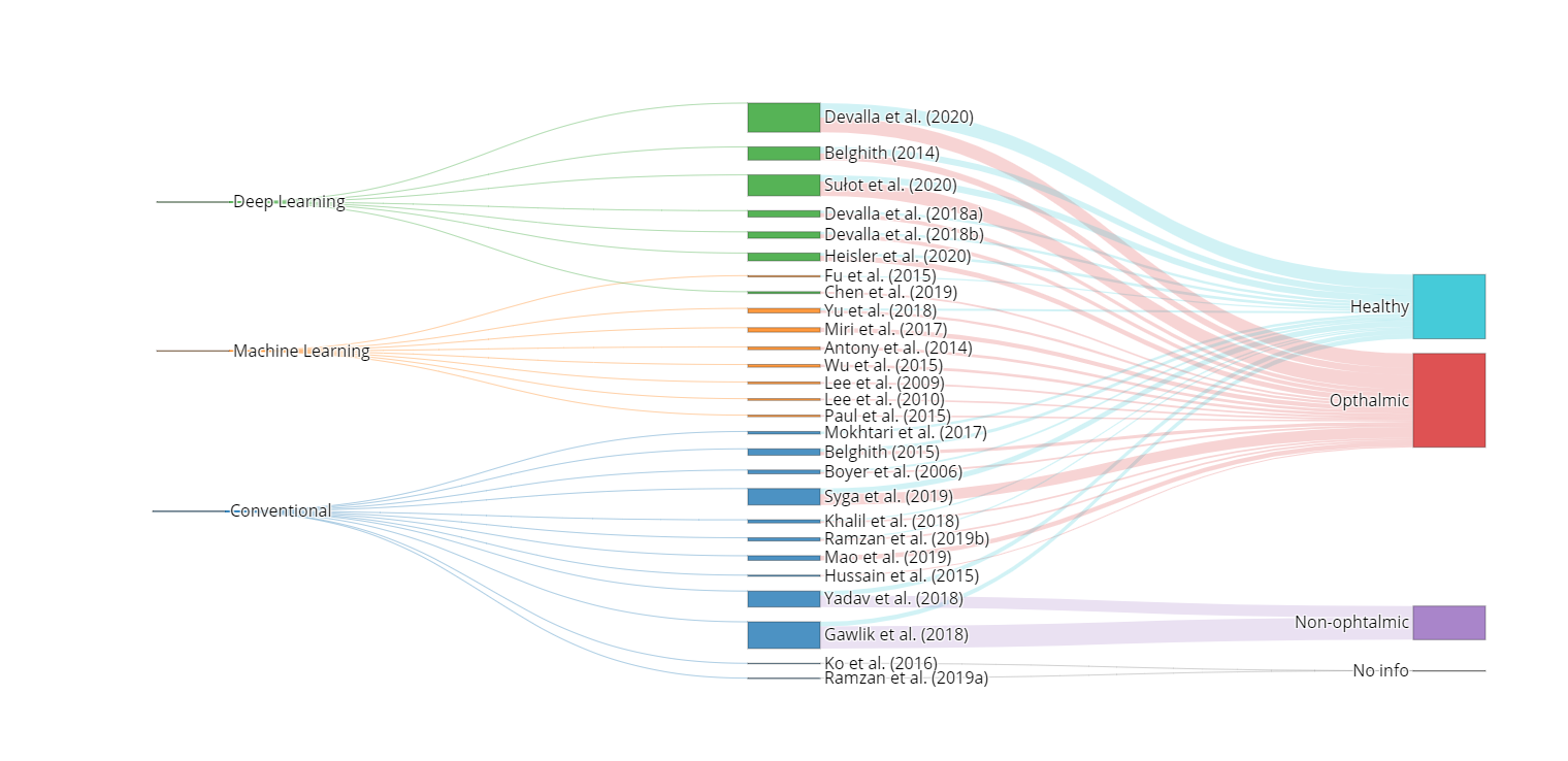
Figure 3: Distribution of the reviewed articles organized by method (deep learning, standard machine learning, and conventional image processing) and the type of data used for developing the algorithm (healthy subjects, patients with ophthalmic diseases, and patients with non-ophthalmic diseases). The height of the boxes is proportional the dataset size.

The table in the Appendix gives a complete overview of all included studies and their characteristics. The distribution of the papers over the three different categories and the size of the dataset used from ophthalmic and non-ophthalmic patients and healthy subjects in all studies can be found in Figure 3.

Analysing Figure 3 it is possible to observe that, overall, deep learning methods use larger datasets.

Most of the reviewed works evaluated the proposed algorithms in pathological data. The only exceptions were (Mokhtari et al., 2017), which validated their method on 40 healthy eyes, and (Ko et al., 2016), which does not specify if the dataset consists of healthy or pathological data. Both authors compare parameters measured in the automatic approaches with manual quantifications.

Among the rest of the works, glaucoma is the most studied pathology. There are only two works that validate their approaches in pathologies other than glaucoma, (Yadav et al., 2018) and (Gawlik et al., 2018), whom applied their method in data from healthy subjects and patients suffering from IIH, MS, NMOSD, and ON.

3.1 Structures of interest

Depending on the aim of the work, different regions or points of interest are segmented in the images. To define these points, two manual segmentations of the ONH region in OCT images can be found in Figures 4 and 5 (boundary- and region-based, respectively). Specifically, Figure 4 shows the ILM anterior surface, the RPE layer and its endpoints, the BM and its opening points, and the LC anterior surface. The vitreal-retinal boundary is equivalent to the anterior surface of the ILM layer (shown in yellow).

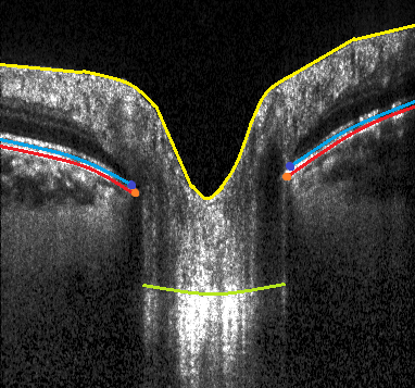
Figure 4: OCT B-scan (Heidelberg Engineering, Germany) showing a manual boundary-based segmentation of the ONH. In yellow, the ILM anterior surface; in light blue, the RPE layer; in dark blue, the RPE endpoints; in red, the Bruch’s membrane; in orange, the Bruch’s membrane opening points; in green, the LC anterior surface.

Figure 5 shows the lower boundary of the RNFL, and the LC. Moreover, it depicts the choroid boundaries. The outer limits of the ONH match the retinal-choroidal boundary endpoints.

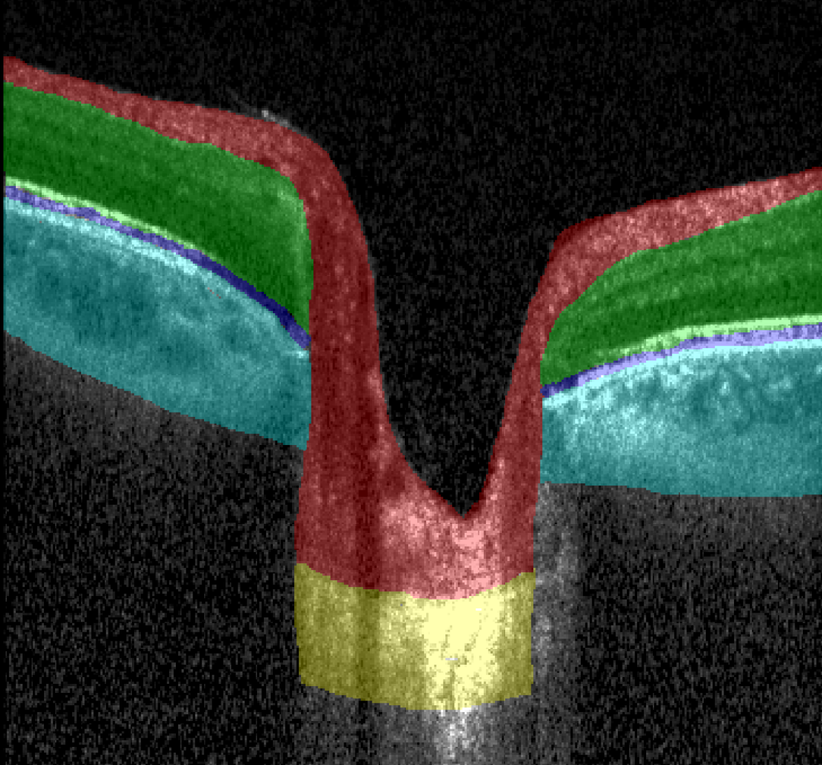
Figure 5: OCT B-scan (Heidelberg Engineering, Germany) showing a manual region-based segmentation of the ONH. In red, the RNFL; in green, all retinal layers between the ganglion cell and the photoreceptor layers; in dark blue, the RPE; in light blue, the choriocapillaris and choroid; and in yellow, the LC.

In the following subsections, a detailed analysis on the approach used by each algorithm to segment the ONH is provided.

3.2 Conventional

Conventional methods are unsupervised segmentation techniques that rely on image processing methods such as thresholding, edge detection and morphological operations.

3.2.1 Thresholding

Thresholding algorithms segment the image based on quantifiable features like image intensity or gradient magnitude, and divide the pixels according to a defined threshold.

Ramzan et al. in (Ramzan et al., 2018) and (Ramzan et al., 2019), and Khalil et al. (Khalil et al., 2018) proposed methods to extract the CDR through the segmentation of the ILM using intensity thresholds. In (Ramzan et al., 2018), the ILM was extracted using intensity based thresholding, followed by interpolation to fill in the gaps. Next, the RPE was obtained with Otsu thresholding. Additionally, a novel thresholding approach was introduced. This approach computes the distance to all the centroids of all the objects to remove the extended cup region. In (Ramzan et al., 2019) only the ILM was used to calculate the CDR. Again, intensity based thresholding was used to detect the ILM, defining its anterior surface as the first non-zero layer. Interpolation was applied to fill the gaps of the extracted layer. Finally, Khalil et al. (Khalil et al., 2018) proposed a method to calculate the CDR from the ILM segmentation using intensity thresholding, with a refinement that includes interpolation of missing points, outliers removal, low quality image and RPE feature analysis.

Mokhtari et al. (Mokhtari et al., 2017) used a different approach, applying ridgelet transform (Candès and Donoho, 1999) for RPE detection and, subsequently, a threshold to determine the RPE boundary location.

Boyer et al. (Boyer et al., 2006) combined thresholding and an adapted Markov model. First, the vitreal-retinal boundary was found through an edge based threshold. A smoothness constraint, that models a priori knowledge about the expected outcome of a successful segmentation, was introduced. On most images, below the retinal-vitreal boundary there are two strong dark-to-light edges that can be used to identify outer limits of the ONH. These contrasts were used by a Markov model (Koozekanani et al., 2001) to extract the full retinal-choroidal boundary.

Also based on edge detection, are the works by Ko et al. (Ko et al., 2016) and Mao et al. (Mao et al., 2019), that used a Canny edge detector as a starting point. In (Ko et al., 2016), Canny edge filter was used to segment the ONH surface. After smoothing the surface with a robust version of the local regression, using weighted linear least squares and a second degree polynomial model, each B-scan was re-mapped into a 3D Cartesian domain where the ONH and BMO surface profiles were fitted with an existing surface modeling tool (Errico, 2006; D’Errico, 2021). In (Mao et al., 2019), 2D and 3D Canny edge detectors were applied to the interpolated 3D volume. They used a minimum-cost-path approach, where the cost map was derived from the edge map and the weighted intensity gradients (based on previous knowledge of the LC anatomy). The locations with large values of intensity gradient yield the detection the LC border.

3.2.2 Active contours

In active contours methods, an object is segmented by an energy-minimizing contour guided by the surrounding pixels. The internal energy comes from the continuity and smoothness of a curve, and the external energy is derived from the edge map of an image (Cheng et al., 2020).

Three of the reviewed works are in this category, two of which (Yadav et al., 2018; Gawlik et al., 2018) applied Chan-Vese level set approach (Chan and Vese, 2001) as a final step of the method. In (Yadav et al., 2018), active contours were used to upgrade their previous 2D segmentation (Kadas et al., 2012) into a robust 3D segmentation of the ONH. They represented the 3D ONH shape using triangulated mesh surfaces of the ILM, RPE and BMO points. The identification of the RPE lower boundary employs a two-stage thin-plate spline fitting that preserves the retinal natural curvature. Finally, the ILM was detected with the Chan-Vese level set approach. The method presented by Gawlik et al. (Gawlik et al., 2018) presents an extended version of (Yadav et al., 2018) by adding a local intensity fitting energy step in order to handle inhomogeneous image intensities.

The third approach based on active contours is the method proposed by Syga et al. (Syga et al., 2019), which automatically segmented the LC in 3D. Otsu thresholding, morphological operators and interpolation were used to estimate the 3D region of interest in fundus photographs. The obtained information was used to define the elliptic cylindrical region of interest along the z-axis of a cuboid made of B-scans. After ILM and BM segmentation, in each OCT scan, active contours were used to reconstruct the 3D segmentation and find the LC.

3.2.3 Graph based methods

Graph based methods represent images as a weighted graph, with the pixels of an image as nodes and the relation between the pixels as the arcs or edges of the graph (Singhal and Verma, 2016).

Hussain et al. (Hussain et al., 2015) introduced the approximate location of TBMR layers and layers veto (a weight based on the layers pattern) as a parameter of the graph weight function. The goal of their work was to segment the ONH and compute the BMO-MRW for glaucoma diagnosis. The TBMR layers are the three most reflective layers of the retina corresponding to the RNFL, the outer neural layer, and the RPE and were detected to limit the search space.

Belghith et al. (Belghith et al., 2015) proposed a new method to segment the anterior LC surface that is able to include prior knowledge in the inference model. They used the MRF class of Bayesian methods. For segmentation, the LC surface was iteratively refined following a perturbation-based approach inspired by the Biased and Filtered Point Sampling method (Chang and Fisher, 2011) according to a non-local MRF energy function.

3.3 Machine Learning

Machine-learning methods train the algorithm to find patterns and features in large amounts of data in order to make decisions and predictions based on new data. They are usually applied after, or in combination with, conventional methods.

Several methods in this section use machine learning after a graph search approach. That is the case of the approach followed by Lee et al. (Lee et al., 2009, 2010), who developed a fast multiscale extension of 3D graph search to detect four intra-retinal surfaces in ONH centered OCT volumes. The authors used a k-NN classifier combined with hull fitting, to segment the ONH cup and neuroretinal rim while preserving their shape. The method assigns one of three labels (background, cup, rim) to each column within the OCT scan. Then, a set of 15 features was calculated for each voxel column in the volume, and used as input for the k-NN classifier.

Antony et al. (Antony et al., 2014), Miri et al. (Miri et al., 2017), and Yu et al. (Yu et al., 2018) all used a random forest classifier (Breiman, 2001) in combination with the graph search approach.

In (Antony et al., 2014), an existing graph theoretic approach (Garvin et al., 2009) was adapted for simultaneous segmentation of multiple continuous surfaces, in order to make it able to identify the ONH boundary in 3D. An iterative method finds the optimal set of feasible surfaces for each estimate of the ONH boundary columns by solving a minimum-closure problem in a graph. The random forest classifier was then trained to find the neural canal opening boundary points, based on the previously learned textural features. However, the continuation of the iterative search on the border of the BM was a common mistake that lead to a wrong placement of the BMO and, consequently, of the borders of the ONH. This limitation was addressed in (Miri et al., 2017) by eliminating the iteration phase. The new method, instead of using a mathematical model for the BMO points, computes the likelihood of each voxel being a BMO point using the random forest classifier.

The method described in (Yu et al., 2018) includes locally adaptive constraints for a more accurate ONH region detection. The ONH region was first detected by random forest method on polar-transformed images with features representing both textural and structural information. Then two layer segmentation methods with locally adaptive constraints, Otsu segmentation guided graph search and shared-hole graph search, were proposed for the segmentation of nine surfaces.

The three remaining papers of this section proposed all different approaches. Fu et al. (Fu et al., 2015) detects the OD through the segmentation of the RPE. A low-rank dictionary based on intensity features and local binary patterns was learned and used to reconstruct the layer on the candidate region. The resulting error curves, that represent the deviations from the smooth geometrical structure, allowed for the boundaries of the OD to be detected. Paul et al. (Paul et al., 2015) performed a segmentation of the retinal and vitreal boundary from OCT ONH centered images by incorporating a GMM (Reynolds, 2009) clustering into a kernel. Finally, Wu et al. (Wu et al., 2015) started by using a multi-scale 3D graph search approach to segment the RPE, followed by a search patch method to segment the ONH. A SVM classifier was trained with the purpose of finding the most likely patch centered at the neural canal opening. The features extracted for patch description were the local binary pattern and histogram of gradient.

3.4 Deep Learning

Deep learning methods are an advanced type of machine-learning algorithms that have been gaining visibility in the last decade. Following computational developments, they are capable of extracting and classifying features automatically when a large amount of training data is given (Seo et al., 2020). The most commonly used architectures for medical image segmentation are based on the U-net (Ronneberger et al., 2015).

Belghith et al. (Belghith et al., 2014) addressed the segmentation problem by improving an existing machine learning based method by Lee et al. (Lee et al., 2010). In (Lee et al., 2010), the estimation of the layers highly depends on the accuracy of the estimated gradient-based transitions, which can be a major drawback for low quality and noisy images, particularly in the BMO area. To overcome this, the authors proposed the use of a ANN and PCA (Kirby and Miranda, 1996). That way, the elliptical shape of the BM curve can be modeled, obtaining a more accurate estimate of the ONH size.

Among the authors that used a U-net as a basis for their algorithm are Chen et al. (Chen et al., 2019), who proposed a method consisting of three steps. First, a coarse detection based on the RPE layer and ONH segmentation in 2D projection image was applied. Then, a U-net was used to improve the accuracy of the coarse detection. Finally, a post processing algorithm removes the outliers. The loss function was a combination of Dice loss with an area bias and the mean square error loss.

In (Sułot et al., 2020), the aim was to segment the BMO. To that end, three deep learning based approaches were used and compared while evaluating the effect of the input size: an ANN where the input is an A-scan, a patch based CNN method where the input is a group of consecutive A-scans and a U-net where the input is a B-scan.

In (Heisler et al., 2020), the aim was layer segmentation. The proposed method, a semi-supervised GAN (Isola et al., 2017), allowed for the training of the network with smaller datasets while taking advantage of unlabeled scans. Additionally, a Faster Region CNN (Ren et al., 2015) was used to segment the BMO from the volumes.

The last three deep learning approaches, all developed by Devalla et al. (Devalla et al., 2018a, b, 2020), present different architectures for segmentation. The aim in (Devalla et al., 2018a) was to segment six neural and connective tissue structures in OCT images of the ONH: the RNFL and the prelamina, the RPE, the set of remaining retinal layers, the choroid, the peripapillary sclera, and the LC. After pre-processing all B-scans with adaptive compensation (Mari et al., 2013a), they used a two dimensional CNN that was trained with manually segmented images. This approach does not offer a precise separation between the LC and the sclera. This drawback was tackled in (Devalla et al., 2018b), which proposes an architecture combining a U-net and residual blocks. The goal is to extract the same six regions of the ONH by capturing both the contextual and local information while taking advantage of residual connections to improve the flow of the gradient information through the network. When compared to (Devalla et al., 2018a), the results showed that the new architecture performed better for all the tissues except for theRPE, where they performed similarly.

Finally, the work in (Devalla et al., 2020) attempted to address one of the main obstacles for the automatic segmentation of the ONH in the clinical environment: the lack of device-independent segmentation algorithms. One of the key elements of the proposed framework was a pre-processing enhancement step, which makes use of a deep learning network to improve the quality of OCT B-scans and to harmonize image characteristics across OCT devices.

The authors (Devalla et al., 2020) found that the use of 3D CNNs could further improve the reliability of the automatic segmentation by considering depth-wise spatial information from adjacent images. The proposed architecture combined three segmentation CNNs based on the 3D U-net. Each of the three 3D CNNs offered an equally plausible segmentation. However, the segmentation of ambiguous regions, such as the sclera and the LC, can differ considerably between networks with different structures. Therefore, an ensembler was used to combine the predictions from the three networks, giving a more robust segmentation in the end.

3.5 Evaluation and validation

Table 1: Results from the boundary based segmentations.

Outcome	Metrics	Results
BMO	(i) Correlation with ground truth; (ii) Error compared with ground truth; (iii) Mean unsigned error; (iv) Mean signed error; (v) Dice similarity coefficient; (vi) Failure rate; (vii) Mean average precision	(i) 0.93 (Boyer et al., 2006); (ii) 32.03 $\pm$ 58.68 $\mu$m (Mokhtari et al., 2017). 12.4 $\pm$ 12.1 pixels (Fu et al., 2015). 2.8 pixels (normal) and 3.1 pixels (glaucoma) (Paul et al., 2015). 54.18 $\pm$ 53.74 $\mu$m (Hussain et al., 2015). 60.00 $\pm$ 42.00 $\mu$m (Wu et al., 2015). 49.28 $\pm$ 16.78 $\mu$m (Miri et al., 2017). 42.38 $\pm$ 18.33 $\mu$m (Chen et al., 2019). (iii) 61.86 $\pm$ 61.97 $\mu$m (x axis) and 12.40 $\pm$ 11.24 $\mu$m (z axis) (Yadav et al., 2018). 49.53 $\pm$ 30.41 $\mu$m (x axis) and 31.58 $\pm$ 21.06 $\mu$m (z axis) (Antony et al., 2014). 37.98 $\pm$ 14.91 $\mu$m (x axis) and 22.28 $\pm$ 8.58 $\mu$m (z axis) (Miri et al., 2017). 9.80 $\pm$ 31.90 $\mu$m (Sułot et al., 2020). 0.023 mm (Lee et al., 2009). 0.026 mm (Lee et al., 2010) (iv) -7.69 $\pm$ 87.27 $\mu$m (x axis) and -1.41 $\pm$ 16.69 $\mu$m (z axis) (Yadav et al., 2018). 26.49 $\pm$ 40.22 $\mu$m (x axis) and 25.45 $m$ 14.37 $\mu$m (z axis) (Antony et al., 2014). -9.49 $\pm$ 24.58 $\mu$m (x axis) and 8.33 $\pm$ 17.72 $\mu$m (z axis) (Miri et al., 2017). (v) 0.925 $\pm$ 0.030 (Yu et al., 2018). 0.959 $\pm$ 0.032 (Sułot et al., 2020). 0.65 $\pm$ 0.14 (Lee et al., 2010). (vi) 0 in 92.5% of the scans (Belghith et al., 2014) (vii) 0.8547 for glaucoma and 0.9567 for control subjects (Heisler et al., 2020).
BMO-MRW	(i) Mean unsigned error; (ii) Mean signed error; (iii) RMSE	(i) 58.62 $\pm$ 43.12 $\mu$m (Hussain et al., 2015). 26.65 $\pm$ 13.27 $\mu$m (Antony et al., 2014). 22.22 $\pm$ 5.99 $\mu$m (Miri et al., 2017). (ii) 6.61 $\pm$ 18.59 $\mu$m (Antony et al., 2014). -0.30 $\pm$ 12.44 $\mu$m (Miri et al., 2017). (iii) 17.99 $\pm$ 8.15 $\mu$m (Antony et al., 2014). 11.62 $\pm$ 4.63 $\mu$m (Miri et al., 2017)
Optic Cup	(i) Correlation with ground truth; (ii) Error compared with ground truth; (iii) Mean unsigned error; (iv) Dice similarity coefficient	(i) 0.80 (Boyer et al., 2006) (ii) 3.4 pixels (normal) and 3.6 pixels (glaucoma) (Paul et al., 2015) (iii) 0.009 mm (Lee et al., 2009). 0.038 mm (Lee et al., 2010) (iv) 0.85 $\pm$ 0.06 (Lee et al., 2010)
CDR	(i) Error compared with ground truth; (ii) Sensitivity; (iii) Specificity; (iv) Accuracy	(i) 0.045 $\pm$ 0.033 (Wu et al., 2015) (ii) 86.2 $\pm$ 7.1% (Khalil et al., 2018) (iii) 86.2 $\pm$ 9.8% (Khalil et al., 2018) (iv) 85.5 $\pm$ 5.2% (Khalil et al., 2018)
ILM	(i) Mean unsigned error; (ii) Mean Dice coefficient; (iii) Error compared with ground truth; (iv) Mean Euclidean distance error	(i) 5.38 $\pm$ 4.23 $\mu$m (Yu et al., 2018). (ii) 0.97 (Heisler et al., 2020). (iii) 4.80 $\mu$m (Gawlik et al., 2018) (iv) 7.08 $\pm$ 3.7 pixels (Ramzan et al., 2018). 7.03 $\pm$ 3.72 pixels
LC	(i) Failure rate; (ii) Accuracy	(i) 0 in 73.7% of the scans (Belghith et al., 2015) (ii) 90.6% (Mao et al., 2019)
ONH surface depth	(i) Error compared with ground truth	(i) 0.7 $\pm$ 1.0 % (Ko et al., 2016).

A summary of the most representative results of the reviewed works can be found in Tables 1 and 2. Several outcomes can be used to evaluate a segmentation. These outcomes can be either a segmented tissue, such as the ILM, the LC, the RNFL, the RPE, the other retinal layers and the choroid, or it can be a biomarker related to a segmented tissue, such as the BMO and optic cup detection, the BMO-MRW, the CDR and the ONH surface depth. For each of these outcomes the metrics used for their evaluation and the quantitative results reported are presented.

One of the metrics mentioned in table 1 is the failure rate. This metric was proposed by Belghith et al. (Belghith et al., 2014, 2015) and it compares the automatic segmentation with the ground truth. A failure rate of 0 is obtained when the mean difference $<$3 pixels, of 1 when the mean difference $<$5 pixels and of 2 when the mean difference $>$5 pixels.

Table 2: Results from the region based segmentation

Outcome	Metrics	Results
RNFL + prelamina	(i) Dice coefficient; (ii) Sensitivity; (iii) Specificity; (iv) Accuracy	(i) 0.82 $\pm$ 0.05 (Devalla et al., 2018c). 0.92 $\pm$ 0.05 for healthy and 0.92 $\pm$ 0.03 for glaucoma (Devalla et al., 2018b). (ii) 0.89 $\pm$ 0.04 (Devalla et al., 2018c) (iii) 0.99 (Devalla et al., 2018c). 0.99 (Devalla et al., 2018b). (iv) 0.93 $\pm$ 0.02 (Devalla et al., 2018c)	Mean for all tissues: (ii) 0.94 $\pm$ 0.02 (Spectralis), 0.93 $\pm$ 0.02 (Cirrus) and 0.93 $\pm$ 0.02 (RTVue) (Devalla et al., 2020). (iii) 0.99 for Spectralis, Cirrus and RTVue (Devalla et al., 2020).
RPE	(i) Dice coefficient (ii) Sensitivity; (iii) Specificity; (iv) Accuracy	(i) 0.84 $\pm$ 0.02 (Devalla et al., 2018c). 0.83 $\pm$ 0.04 for healthy and 0.84 $\pm$ 0.03 for glaucoma (Devalla et al., 2018b). (ii) 0.90 $\pm$ 0.03 (Devalla et al., 2018c) (iii) 0.99 (Devalla et al., 2018c). 0.99 (Devalla et al., 2018b). (iv) 0.93 $\pm$ 0.02 (Devalla et al., 2018c)
Other retinal layers	(i) Dice coefficient (ii) Sensitivity; (iii) Specificity; (iv) Accuracy	(i) 0.86 $\pm$ 0.03 (Devalla et al., 2018c). 0.95 $\pm$ 0.01 for healthy and 0.96 $\pm$ 0.03 for glaucoma (Devalla et al., 2018b). (ii) 0.98 $\pm$ 0.02 (Devalla et al., 2018c) (iii) 0.99 (Devalla et al., 2018c). 0.99 (Devalla et al., 2018b). (iv) 0.98 $\pm$ 0.01 (Devalla et al., 2018c)
Choroid	(i) Dice coefficient (ii) Sensitivity; (iii) Specificity; (iv) Accuracy	(i) 0.85 $\pm$ 0.02 (Devalla et al., 2018c). 0.90 $\pm$ 0.03 for healthy and 0.91 $\pm$ 0.05 for glaucoma (Devalla et al., 2018b). (ii) 0.91 $\pm$ 0.02 (Devalla et al., 2018c) (iii) 0.99 (Devalla et al., 2018c). 0.99 (Devalla et al., 2018b). (iv) 0.93 $\pm$ 0.01 (Devalla et al., 2018c)

Even though three works reported a region segmentation of the LC (Devalla et al., 2018b, c, 2020), no values are reported in Table 2. Given the subjectivity in the visibility of the posterior LC boundary, the groups were only able to do a qualitative assessment of this the segmentation of the LC.

From the analysed pool, two of the works studied not only if the qualify of the segmentation was good, but also if the parameters obtained from the automatic segmentation were able to correctly classify data from the different groups. Ramzan et al. (Ramzan et al., 2018) evaluated the performance of the computed CDR in separating healthy from glaucomatous eyes, and it showed an average sensitivity of 87%, specificity of 73%, and accuracy of 79%. Syga et al. (Syga et al., 2019) validated their model on a dataset from 255 subjects, obtained a 68% accuracy and 0.66 AUC in distinguishing POAG patients from controls (p-value $<$0.001), 64% and 0.585 between suspects with GODA and controls (p-value $<$0.015), and 56% and 0.561 between patients and suspects (p-value $=$ 0.333) based on the mean LC index (total shape of the LC parameterization based on the fourth-order polynomial fit).

4 Discussion

The present review collects and summarizes the existing automatic algorithms for the segmentation of the ONH in OCT scans. It shows that improvements are necessary in the field since there is a limited number of studies, with great diversity in the size and type of datasets used, segmented regions and validation methods, which precludes a comparison between studies. Boundary segmentation was the starting point for the detection of the ONH and its layers. However, as methods developed, region segmentation has also been proposed.

Conventional methods focused mainly on segmenting boundaries, through the detection of BMO points, the ILM and the RPE limits. For the LC, only the anterior surface could be detected, which limited the parameters that could be extracted with these methods.

In medical imaging segmentation tasks, it is often assumed that the surfaces are continuous, which is not the case for the ONH in which surfaces converge to a hole. This can be a problem when segmenting structures with multiple interacting surfaces, such as in OCT volumes of the ONH.

Since machine-learning methods were mostly applied after conventional methods, they were often able to address segmentation problems that had remained unanswered with prior methods. Particularly, for accurately identifying the optic cup, for which pattern recognition played an important role. Miri et al. (Miri et al., 2017) were able to improve the unsigned border error of BMO-MRW from previous methods by at least 4 $\mu$m (26.65 $\pm$ 13.27 $\mu$m and 22.22 $\pm$ 5.99 $\mu$m).

Deep learning methods have been gaining visibility for their success in other medical imaging processing and analysis, and can be the future of research in this field (Rizwan I Haque and Neubert, 2020). Using deep learning, (Chen et al., 2019) was able to outperform the mean error of previous BMO segmentation by at least 7 $\mu$m. Moreover, only deep learning based algorithms have been able to perform a region segmentation of several tissues of the ONH. Devalla et al. were able to accurately segment almost all connective and neural tissues with sensitivities and specificities around or above 90%, except for the LC, that despite improvements, remains a challenge due to low signal-to-noise ratio.

Connective tissues, such as the peripapillary sclera, BM and the LC are the main load bearing elements of the ONH. Parameters extracted from the segmentation of these type of tissues have already proven to make a difference in several diagnoses (Yang et al., 2015). The LC load-bearing connective tissue components comprise about 40% of the tissue volume in the laminar region of the ONH (Downs and Girkin, 2017). Adding to its anatomical location, the LC becomes a weak spot with the conflicting tasks of providing structural and nutrient support to the axons while withstanding mechanical strain (Downs and Girkin, 2017). When compressed above a certain point, the LC can be deformed, compromising axonal transport and tissue remodeling by reactive astrocytes (Lee et al., 2017), as well as the diffusion of nutrients from the capillaries (Burgoyne et al., 2005). Several studies have already shown that LC features, such as LC depth and thickness, have potential to be used in clinical diagnosis (Paulo et al., 2021). Moreover, being significantly different between healthy patients and ocular and systemic pathologies while being patient-specific features (Paulo et al., 2021), LC features are seen as increasingly promising for patient follow-up as well. Therefore, the remaining lack of accuracy in detecting the LC can affect diagnosis and follow-up.

Altogether, the values of the parameters extracted from the segmentations showed significant differences between healthy and pathological groups. Methods such as the ones developed by Ramzan et al. (Ramzan et al., 2018) and Syga et al. (Syga et al., 2019) already achieved sensitivities of 87% and 81% in distinguishing healthy from pathological groups.

Datasets with data from less than 40 patients were often used. Even though a lot of imaging data are being acquired in clinical practice, these data are rarely labelled and/or publicly available. The time consuming process of manual labelling by experts, combined with the scarcity of publicly available segmented datasets, may cause further delays in technology development, since time is lost in repeating steps that have already been done and validated by previous groups. This is particularly problematic for supervised deep learning methods since they need more data to yield accurate results. However, future work may focus on label-free/unsupervised learning since it will ease the burden of manual labelling (however, it will not solve the lack of OCT data itself). Therefore, efforts to make more clinical data available and create sharing practices/protocols between groups could further accelerate research, allowing more studies to be done more effectively, which will close the gap to automation in the clinic.

One limitation of this review is that, since the literature search was made on MEDLINE (Pubmed) and Scopus bibliographic databases only, some technical studies might have been missed. By considering only articles with detailed descriptions on the algorithm used, the number of included articles was shortened since otherwise a review of the method would not be possible. Moreover, studies which were solely published as congress abstracts were excluded from this review.

5 Conclusion

There is a growing interest in ONH features as biomarkers for disease diagnosis and/or progression. This review highlights algorithms that automatically segment several structures and boundaries from ONH centered OCT scans. From these automatic segmentations, several parameters can be automatically extracted which may be relevant for clinical practice. Nevertheless, efforts should be employed to make more OCT data available, develop standardized guidelines for the extracted parameters and metrics used in the validation of the algorithms so that more accurate comparisons between methods can be performed. Moreover, efforts in improving LC signal-to-noise ratio and device-independent algorithms can contribute to a better diagnosis and follow-up of ONH-related diseases in daily clinical practice.

Table 3: Characteristics of the reviewed studies

Category	Authors	Dataset	Regions Segmented	Validation	Results	Technique	Device
Conventional	Boyer et al. [2006]	59 glaucoma B-scans	Retinal-vitreal boundary, limits of the OD, retinal-choroid boundaries.	Comparison with the ground truth.	High correlation between automatic and manual cup and disk limits.	-	OCT 3000 from Zeiss-Humphrey
Conventional	Hussain et al. [2015]	13 glaucoma scans	ILM, BMO, HRC, RNFL, RPE, OD boundary	Comparison with ground truth and existing method. Confusion matrix based metrics. Distance metrics.	Robust segmentation over noise and pathology.	SD-OCT	Spectralis
Conventional	Belghith et al. [2015]	50 healthy scans and 50 glaucoma scans	LC anterior surface	Comparison with ground truth. Statistical tests.	High similarity between manual and automatic segmentation. Significant correlation between changes in IOP and the position of the LC.	EDI SD-OCT	Spectralis
Conventional	Ko et al. [2016]	no info	ILM, BMO	Comparison with ground truth.	Accurate segmentation of the ONH structure. Not sensitive to the differentiation of blood vessels from the ONH surface.	SD-OCT	Spectralis
Conventional	Mokhtari et al. [2017]	40 healthy scans	RPE break points, RPE boundary	Comparison with ground truth.	Accurate segmentation of the OD boundary.	no info	Topcon model of 3D-1000 unit
Conventional	Gawlik et al. [2018]	71 healthy scans and 345 pathological scans (31 IIH + 60 NMOSD + 252 MS)	ILM	Statistical tests. Comparison with segmentation from a device. Distance metrics. Visual evaluation.	Robust segmentations over variations in ONH topology. Outperforms device segmentation.	SD-OCT	Spectralis
Conventional	Khalil et al. [2018]	22 healthy scans and 28 glaucoma scans	ILM and RPE	Comparison with ground truth. Comparison with computed generated values. Comparison with existing methods Wang et al. [2013], Nithya and Venkateswaran [2015], Babu et al. [2015].	Outperforms existing methods and computer generated values.	SD-OCT	no info
Conventional	Yadav et al. [2018]	71 healthy scans and 177 pathological scans (31 IIH +146 autoimmune central nervous system disorders )	RPE, BMO Points, ILM and BMO.	Comparison with ground truth. Distance metrics.	Successfully captures the differences between pathological groups.	SD-OCT	Spectralis
Conventional	Ramzan et al. [2018]	50 scans from healthy and glaucoma patients	ILM and RPE	Comparison with ground truth. comparison with computer generated values. Confusion matrix based metrics.	High correlation with ground truth. Outperforms existing techniques.	TOPCON’S 3D OCT-1000
Conventional	Ramzan et al. [2019]	50 scans from healthy and glaucoma patients	ILM	Comparison with ground truth. Distance metrics. Visual evaluation.	Accurate segmentation.	SD-OCT	Topcon
Conventional	Syga et al. [2019]	86 healthy scans and 169 glaucoma scans	ILM, BM points and LC	Statistical tests. Confusion matrix based metrics.	Statiscally significant differences between glaucoma patients (POAG and GODA) and healthy controls. The mean LC shapes for POAG and GODA were not significantly different.	EDI OCT	Spectralis
Conventional	Mao et al. [2019]	72 glaucoma scans	LC anterior surface	Comparison with ground truth. Visual evaluation.	Segmentation accuracy is significantly higher when a deep learning noise reduction algorithm is used than in raw images.	SS-OCT	Topcon
Machine learning	Lee et al. [2009]	30 glaucoma scans	3 intraretinal surfaces, OD boundary	Comparison with ground truth. Distance metrics.	No signifficant differences between the unsigned errors of the optic cup and disk, before and after feature selection.	HD-OCT	Cirrus
Machine learning	Lee et al. [2010]	27 glaucoma scans	4 intraretinal surfaces, OD boundary	Comparison with the ground truth. Distance metrics. Confusion matrix based metrics.	Contextual 9-k-NN outperforms the regular k-NN classifier when no post processing is applied. Performance of 9-k-NN classifier is significantly better with post processing.	HD-OCT	Cirrus
Machine learning	Antony et al. [2014]	44 glaucoma scans	BM, intraretinal surfaces, ONH hole	Comparison with ground truth and existing methods. Distance metrics. Confusion matrix based metrics.	Outperforms existing methods Hu et al. [2010], Lee et al. [2010].	SD-OCT	Cirrus
Machine learning	Wu et al. [2015]	42 glaucoma scans	ILM, RPE	Comparison with ground truth and existing method. Distance metrics. Confusion matrix based metrics.	Outperforms existing methods Lee et al. [2010].	SD-OCT	Cirrus
Machine learning	Fu et al. [2015]	48 healthy scans	ILM, RPE, OD boundary	Comparison with ground truth and other methods.	Outperforms existing methods Boyer et al. [2006].	SD-OCT	Topcon
Machine learning	Paul et al. [2015]	25 glaucoma B-scans	Retinal layers, OD boundary	Comparison with ground truth.	Correct segmentation in normal and glaucoma affected images.	no info	no info
Machine learning	Miri et al. [2017]	69 glaucoma scans	ILM, (IS/OS), BM	Comparison with ground truth and existing methods. Distance metrics. Statistical tests.	Outperforms existing methods Antony et al. [2014].	HD-OCT	Cirrus
Machine learning	Yu et al. [2018]	30 healthy scans and 35 glaucoma scans	RNFL, retinal layers, RPE/Bruch’s complex and OD boundary	Comparison with ground truth and existing methods. Confusion matrix based metrics. Distance metrics.	Outperforms existing methods Hu et al. [2009], Zang et al. [2017].	SD-OCT	Topcon
Deep learning	Belghith et al. [2014]	100 healthy scans and 105 glaucoma scans	BM	Comparison with ground truth, values from the device and other methods. Statistical tests.	High correlation with ground truth and built-in software of the device. Significant differences between glaucoma and healthy eyes.	EDI SD-OCT	Cirrus and Spectralis
Deep learning	Devalla et al. [2018c]	40 healthy scans and 60 glaucoma scans	RNFL and the prelamina; RPE; all other retinal layers; the choroid; the peripapillary sclera and the LC;	Confusion matrix based metrics. Statistical tests.	Good performance for all tissues in glaucoma and healthy images. Performs better with compensated images.	EDI SD-OCT	Spectralis
Deep learning	Devalla et al. [2018b]	40 healthy scans and 60 glaucoma scans	RNFL and the prelamina; RPE; all other retinal layers; choroid; peripapillary sclera; LC;	Confusion matrix based metrics.	Good performance for all tissues in glaucoma and healthy images. No significant differences in segmentation performances with compensated and uncompensated images.	EDI OCT	Spectralis
Deep learning	Chen et al. [2019]	30 glaucoma scans	OD boundary, RPE, BMO points	Comparison with the ground truth and with existing methods.	Outperforms existing methods Hussain et al. [2015], Wu et al. [2015], Miri et al. [2017].	SD-OCT	Topcon
Deep learning	Heisler et al. [2020]	42 healthy scans and 80 glaucoma scans	ILM, RNFL, BM, choroid-sclera boundary; BMO points	Comparison with ground truth. Confusion matrix based metrics. Statistical tests.	No statistically significant difference between BMO segmentation and ground truth. Thickness parameters were highly correlated.	SS-OCT	custom-built OCT
Deep learning	Devalla et al. [2020]	225 healthy scans and 225 glaucoma scans	RNFL and prelamina; ganglion cell complex; all other retinal layers; RPE; choroid; LC	Confusion matrix based metrics. Visual evaluation. Statistical tests.	Networks trained in any of the devices, successfully segmented images from other devices with high performances in all tissues.	SD-OCT	Spectralis, Cirrus and RTVue
Deep learning	Sułot et al. [2020]	102 healthy scans and 223 glaucoma scans	BMO	Comparison with ground truth. Confusion matrix based metrics. Distance metrics.	U-net like architecture with B-scans as input had the best performance.	SD-OCT	Spectralis

References

- Antony et al. [2014] Bhavna J Antony, Mohammed S Miri, Michael D Abràmoff, Young H Kwon, and Mona K Garvin. Automated 3d segmentation of multiple surfaces with a shared hole: segmentation of the neural canal opening in sd-oct volumes. In International Conference on Medical Image Computing and Computer-Assisted Intervention, pages 739–746. Springer, 2014.
- Babu et al. [2015] TR Babu, S Devi, R Venkatesh, et al. Optic nerve head segmentation using fundus images and optical coherence tomography images for glaucoma detection. Biomedical Papers, 159(4):607–615, 2015.
- Bekkers et al. [2020] Amerens Bekkers, Noor Borren, Vera Ederveen, Ella Fokkinga, Danilo Andrade De Jesus, Luisa Sánchez Brea, Stefan Klein, Theo van Walsum, João Barbosa-Breda, and Ingeborg Stalmans. Microvascular damage assessed by optical coherence tomography angiography for glaucoma diagnosis: a systematic review of the most discriminative regions. Acta ophthalmologica, 98(6):537–558, 2020.
- Belghith et al. [2014] Akram Belghith, Christopher Bowd, Robert N Weinreb, and Linda M Zangwill. A hierarchical framework for estimating neuroretinal rim area using 3d spectral domain optical coherence tomography (sd-oct) optic nerve head (onh) images of healthy and glaucoma eyes. In 2014 36th Annual International Conference of the IEEE Engineering in Medicine and Biology Society, pages 3869–3872. IEEE, 2014.
- Belghith et al. [2015] Akram Belghith, Christopher Bowd, Felipe A. Medeiros, Robert N. Weinreb, and Linda M. Zangwill. Automated segmentation of anterior lamina cribrosa surface: How the lamina cribrosa responds to intraocular pressure change in glaucoma eyes? Proceedings - International Symposium on Biomedical Imaging, 2015-July:222–225, 2015. ISSN 19458452. doi: 10.1109/ISBI.2015.7163854.
- Boyer et al. [2006] Kim L. Boyer, Artemas Herzog, and Cynthia Roberts. Automatic recovery of the optic nervehead geometry in optical coherence tomography. IEEE Transactions on Medical Imaging, 25(5):553–570, 2006. ISSN 02780062. doi: 10.1109/TMI.2006.871417.
- Breiman [2001] L Breiman. Random Forests. Machine Learning, 45:5–32, 2001. doi: 10.1023/A:1010933404324.
- Burgoyne et al. [2005] Claude F. Burgoyne, J. Crawford Downs, Anthony J. Bellezza, J. K. Francis Suh, and Richard T. Hart. The optic nerve head as a biomechanical structure: A new paradigm for understanding the role of IOP-related stress and strain in the pathophysiology of glaucomatous optic nerve head damage. Progress in Retinal and Eye Research, 24(1):39–73, 2005. ISSN 13509462. doi: 10.1016/j.preteyeres.2004.06.001.
- Cabrera DeBuc et al. [2019] Delia Cabrera DeBuc, Magdalena Gaca-Wysocka, Andrzej Grzybowski, and Piotr Kanclerz. Identification of Retinal Biomarkers in Alzheimer’s Disease Using Optical Coherence Tomography: Recent Insights, Challenges, and Opportunities. Journal of Clinical Medicine, 8(7):996, 2019. ISSN 2077-0383. doi: 10.3390/jcm8070996.
- Candès and Donoho [1999] Emmanuel J. Candès and David L. Donoho. Ridgelets: A key to higher-dimensional intermittency? Philosophical Transactions of the Royal Society A: Mathematical, Physical and Engineering Sciences, 357(1760):2495–2509, 1999. ISSN 1364503X. doi: 10.1098/rsta.1999.0444.
- Chan and Vese [2001] Tony F. Chan and Luminita A. Vese. Active contours without edges. IEEE Transactions on Image Processing, 10(2):266–277, 2001. ISSN 10577149. doi: 10.1109/83.902291.
- Chang and Fisher [2011] Jason Chang and John W Fisher. Efficient mcmc sampling with implicit shape representations. In CVPR 2011, pages 2081–2088. IEEE, 2011.
- Chen et al. [2019] Zailiang Chen, Peng Peng, Hailan Shen, Hao Wei, Pingbo Ouyang, and Xuanchu Duan. Region-segmentation strategy for Bruch’s membrane opening detection in spectral domain optical coherence tomography images. Biomedical Optics Express, 10(2):526, 2019. ISSN 2156-7085. doi: 10.1364/boe.10.000526.
- Cheng et al. [2020] Ke Cheng, Tianfeng Xiao, Qingfang Chen, and Yuanquan Wang. Image segmentation using active contours with modified convolutional virtual electric field external force with an edge-stopping function. PLoS ONE, 15(3):1–14, 2020. ISSN 19326203. doi: 10.1371/journal.pone.0230581. URL http://dx.doi.org/10.1371/journal.pone.0230581.
- De Jesus et al. [2020] Danilo Andrade De Jesus, Luisa Sánchez Brea, João Barbosa Breda, Ella Fokkinga, Vera Ederveen, Noor Borren, Amerens Bekkers, Michael Pircher, Ingeborg Stalmans, Stefan Klein, et al. Octa multilayer and multisector peripapillary microvascular modeling for diagnosing and staging of glaucoma. Translational Vision Science & Technology, 9(2):58–58, 2020.
- D’Errico [2021] John D’Errico. Surface fitting using gridfit matlab central file exchange, 2021. URL http://pt.wikipedia.org/w/index.php?title=BibTeX&oldid=4879810. https://www.mathworks.com/matlabcentral/fileexchange/8998-surface-fitting-using-gridfit, Retrieved March 16, 2021.
- Devalla et al. [2018a] Sripad Krishna Devalla, Khai Sing Chin, Jean-martial Mari, Tin A Tun, G Nicholas, J A Girard, Tin Aung, and Alexandre H Thi. A Deep Learning Approach to Digitally Stain Optical Coherence Tomography Images of the Optic Nerve Head. Invest Ophthalmol Vis Sci., 2018a.
- Devalla et al. [2018b] Sripad Krishna Devalla, Prajwal K. Renukanand, Bharathwaj K. Sreedhar, Shamira Perera, Jean Martial Mari, Khai Sing Chin, Tin A. Tun, Nicholas G. Strouthidis, Tin Aung, Alexandre H. Thiéry, and Michaël J.A. Girard. DRUNET: A dilated-residual u-net deep learning network to digitally stain optic nerve head tissues in optical coherence tomography images. arXiv, 9(7):575–584, 2018b. ISSN 23318422. doi: 10.1364/boe.9.003244.
- Devalla et al. [2018c] Sripad Krishna Devalla, Giridhar Subramanian, Tan Hung Pham, Xiaofei Wang, Shamira Perera, Tin A. Tun, Tin Aung, Leopold Schmetterer, Alexandre H. Thiéry, and Michaël J.A. Girard. A deep learning approach to denoise optical coherence tomography images of the optic nerve head. arXiv, 2018c. ISSN 23318422.
- Devalla et al. [2020] Sripad Krishna Devalla, Tan Hung Pham, Satish Kumar Panda, Liang Zhang, Giridhar Subramanian, Anirudh Swaminathan, Chin Zhi Yun, Mohan Rajan, Sujatha Mohan, Ramaswami Krishnadas, Vijayalakshmi Senthil, John Mark S. de Leon, Tin A. Tun, Ching Yu Cheng, Leopold Schmetterer, Shamira Perera, Tin Aung, Alexandre H. Thiéry, and Michaël J.A. Girard. Towards label-free 3d segmentation of optical coherence tomography images of the optic nerve head using deep learning. arXiv, 11(11):6356–6378, 2020. ISSN 23318422. doi: 10.1364/boe.395934.
- Downs and Girkin [2017] J. Crawford Downs and Christopher A. Girkin. Lamina cribrosa in glaucoma. Current Opinion in Ophthalmology, 28(2):113–119, 2017. ISSN 15317021. doi: 10.1097/ICU.0000000000000354.
- Eraslan et al. [2016] Muhsin Eraslan, Eren Cerman, Sevcan Yildiz Balci, Hande Celiker, Ozlem Sahin, Ahmet Temel, Devran Suer, and Nese Tuncer Elmaci. The choroid and lamina cribrosa is affected in patients with Parkinson’s disease: Enhanced depth imaging optical coherence tomography study. Acta Ophthalmologica, 94(1):e68–e75, 2016. ISSN 17553768. doi: 10.1111/aos.12809.
- Errico [2006] John R D Errico. Understanding Gridfit The mechanical and philosophical underpinnings. Methodology, 1(1):1–6, 2006.
- Fu et al. [2015] Huazhu Fu, Dong Xu, Stephen Lin, Damon Wing Kee Wong, and Jiang Liu. Automatic Optic Disc Detection in OCT Slices via Low-Rank Reconstruction. IEEE Transactions on Biomedical Engineering, 62(4):1151–1158, 2015. ISSN 15582531. doi: 10.1109/TBME.2014.2375184.
- Fujimoto and Swanson [2016] James Fujimoto and Eric Swanson. The development, commercialization, and impact of optical coherence tomography. Investigative Ophthalmology and Visual Science, 57(9):OCT1–OCT13, 2016. ISSN 15525783. doi: 10.1167/iovs.16-19963.
- Garvin et al. [2009] Mona Kathryn Garvin, Michael David Abràmoff, Xiaodong Wu, Senior Member, Stephen R Russell, Trudy L Burns, and Milan Sonka. Automated 3-D Intraretinal Layer Segmentation of Macular Spectral-Domain Optical Coherence Tomography Images. IEEE Trans Med Imaging, 28(9):1436–1447, 2009.
- Gawlik et al. [2018] Kay Gawlik, Frank Hausser, Friedemann Paul, Alexander U. Brandt, and Ella Maria Kadas. Active contour method for ILM segmentation in ONH volume scans in retinal OCT. Biomedical Optics Express, 9(12):6497, 2018. ISSN 2156-7085. doi: 10.1364/boe.9.006497.
- Heisler et al. [2020] Morgan Heisler, Mahadev Bhalla, Julian Lo, Zaid Mammo, Sieun Lee, Myeong Jin Ju, Mirza Faisal Beg, and Marinko V. Sarunic. Semi-supervised deep learning based 3D analysis of the peripapillary region. Biomedical Optics Express, 11(7):3843, 2020. ISSN 2156-7085. doi: 10.1364/boe.392648.
- Hu et al. [2009] Zhihong Hu, Meindert Niemeijer, Kyungmoo Lee, Michael D. Abràmoff, Milan Sonka, and Mona K. Garvin. Automated segmentation of the optic disc margin in 3-D optical coherence tomography images using a graph-theoretic approach. Medical Imaging 2009: Biomedical Applications in Molecular, Structural, and Functional Imaging, 7262:72620U, 2009. ISSN 16057422. doi: 10.1117/12.811694.
- Hu et al. [2010] Zhihong Hu, Michael D Abràmoff, Young H Kwon, Kyungmoo Lee, and Mona K Garvin. Automated segmentation of neural canal opening and optic cup in 3d spectral optical coherence tomography volumes of the optic nerve head. Investigative ophthalmology & visual science, 51(11):5708–5717, 2010.
- Hussain et al. [2015] Md Akter Hussain, Alauddin Bhuiyan, and Kotagiri Ramamohanarao. Disc segmentation and bmo-mrw measurement from sd-oct image using graph search and tracing of three bench mark reference layers of retina. In 2015 IEEE International Conference on Image Processing (ICIP), pages 4087–4091. IEEE, 2015.
- Isola et al. [2017] Phillip Isola, Jun-Yan Zhu, Tinghui Zhou, and Alexei A Efros. Image-to-image translation with conditional adversarial networks. In Proceedings of the IEEE conference on computer vision and pattern recognition, pages 1125–1134, 2017.
- Jesus et al. [2019] Danilo A Jesus, Joao Barbosa Breda, Karel Van Keer, Amândio Rocha Sousa, Luis Abegao Pinto, and Ingeborg Stalmans. Quantitative automated circumpapillary microvascular density measurements: a new angiooct-based methodology. Eye, 33(2):320–326, 2019.
- Kadas et al. [2012] Ella Maria Kadas, Falko Kaufhold, Christian Schulz, Friedemann Paul, Konrad Polthier, and Alexander U. Brandt. 3D optic nerve head segmentation in idiopathic intracranial hypertension. Informatik aktuell, pages 262–267, 2012. ISSN 1431472X. doi: 10.1007/978-3-642-28502-8-46.
- Khalil et al. [2018] Tehmina Khalil, M. Usman Akram, Hina Raja, Amina Jameel, and Imran Basit. Detection of Glaucoma Using Cup to Disc Ratio from Spectral Domain Optical Coherence Tomography Images. IEEE Access, 6:4560–4576, 2018. ISSN 21693536. doi: 10.1109/ACCESS.2018.2791427.
- Kirby and Miranda [1996] Michael J Kirby and Rick Miranda. Circular nodes in neural networks. Neural Computation, 8(2):390–402, 1996.
- Ko et al. [2016] M. W.L. Ko, C. K.S. Leung, and T. Y.P. Yuen. Automated segmentation of optic nerve head for the topological assessment. 2016 Global Medical Engineering Physics Exchanges/Pan American Health Care Exchanges, GMEPE/PAHCE 2016, pages 4–7, 2016. doi: 10.1109/GMEPE-PAHCE.2016.7504611.
- Koozekanani et al. [2001] Dara Koozekanani, Student Member, Kim Boyer, Senior Member, and Cynthia Roberts. Coherence Tomography Using a Markov Boundary Model. IEEE transactions on medical imaging, 20(9):900–916, 2001.
- Lang et al. [2013] Andrew Lang, Aaron Carass, Matthew Hauser, Elias S. Sotirchos, Peter A. Calabresi, Howard S. Ying, and Jerry L. Prince. Retinal layer segmentation of macular OCT images using boundary classification. Biomedical Optics Express, 4(7):1133, 2013. ISSN 2156-7085. doi: 10.1364/boe.4.001133.
- Lee et al. [2009] Kyungmoo Lee, Meindert Niemeijer, Mona K. Garvin, Young H. Kwon, Milan Sonka, and Michael D. Abràmoff. 3-D segmentation of the rim and cup in spectral-domain optical coherence tomography volumes of the optic nerve head. Medical Imaging 2009: Biomedical Applications in Molecular, Structural, and Functional Imaging, 7262:72622D, 2009. ISSN 16057422. doi: 10.1117/12.811315.
- Lee et al. [2010] Kyungmoo Lee, Student Member, Meindert Niemeijer, Mona K Garvin, Young H Kwon, Milan Sonka, and Michael D Abràmoff. Segmentation of the Optic Disc in 3-D OCT Scans of the Optic Nerve Head. IEEE transactions on medical imaging, 29(1):159–168, 2010.
- Lee et al. [2017] Seung Hyen Lee, Tae Woo Kim, Eun Ji Lee, Michaël J.A. Girard, and Jean Martial Mari. Diagnostic power of lamina cribrosa depth and curvature in glaucoma. Investigative Ophthalmology and Visual Science, 58(2):755–762, 2017. ISSN 15525783. doi: 10.1167/iovs.16-20802.
- Lemmens et al. [2020] Sophie Lemmens, Toon Van Craenendonck, Jan Van Eijgen, Lies De Groef, Rose Bruffaerts, Danilo Andrade de Jesus, Wouter Charle, Murali Jayapala, Gordana Sunaric-Mégevand, Arnout Standaert, et al. Combination of snapshot hyperspectral retinal imaging and optical coherence tomography to identify alzheimer’s disease patients. Alzheimer’s research & therapy, 12(1):1–13, 2020.
- Mao et al. [2019] Zaixing Mao, Atsuya Miki, Song Mei, Ying Dong, Kazuichi Maruyama, Ryo Kawasaki, Shinichi Usui, Kenji Matsushita, Kohji Nishida, and Kinpui Chan. Deep learning based noise reduction method for automatic 3D segmentation of the anterior of lamina cribrosa in optical coherence tomography volumetric scans. Biomedical Optics Express, 10(11):5832, 2019. ISSN 2156-7085. doi: 10.1364/boe.10.005832.
- Mari et al. [2013a] Jean Martial Mari, Nicholas G Strouthidis, Sung Chul Park, and J A Girard. Enhancement of Lamina Cribrosa Visibility in Optical Coherence Tomography Images Using Adaptive Compensation. Invest Ophthalmol Vis Sci., pages 2238–2247, 2013a. doi: 10.1167/iovs.12-11327.
- Mari et al. [2013b] Jean Martial Mari, Nicholas G. Strouthidis, Sung Chul Park, and Michaël J.A. Girard. Enhancement of lamina cribrosa visibility in optical coherence tomography images using adaptive compensation. Investigative Ophthalmology and Visual Science, 54(3):2238–2247, 2013b. ISSN 01460404. doi: 10.1167/iovs.12-11327.
- Miri et al. [2017] Mohammad Saleh Miri, Michael D. Abramoff, Young H. Kwon, Milan Sonka, and Mona K. Garvin. A Machine-Learning Graph-Based Approach for 3D Segmentation of Bruch’s Membrane Opening from Glaucomatous SD-OCT Volumes. Medical Image Analysis, 39:206–217, 2017. doi: 10.1016/j.media.2017.04.007.A.
- Mokhtari et al. [2017] Marzieh Mokhtari, Hossein Rabbani, Alireza Mehri-Dehnavi, and Rahele Kafieh. Exact localization of breakpoints of retinal pigment epithelium in optical coherence tomography of optic nerve head. In 2017 39th Annual International Conference of the IEEE Engineering in Medicine and Biology Society (EMBC), pages 1505–1508. IEEE, 2017.
- Nithya and Venkateswaran [2015] R Nithya and N Venkateswaran. Analysis of segmentation algorithms in colour fundus and oct images for glaucoma detection. Indian Journal of Science and Technology, 8(24):1, 2015.
- Park et al. [2012] Hae Young Lopilly Park, So Hee Jeon, and Chan Kee Park. Enhanced depth imaging detects lamina cribrosa thickness differences in normal tension glaucoma and primary open-angle glaucoma. Ophthalmology, 119(1):10–20, 2012. ISSN 01616420. doi: 10.1016/j.ophtha.2011.07.033. URL http://dx.doi.org/10.1016/j.ophtha.2011.07.033.
- Paul et al. [2015] Dincy Paul, S Priya, and T Ashok Kumar. Gmm clustering based segmentation and optic nervehead geometry detection from oct nervehead images. In 2015 Global Conference on Communication Technologies (GCCT), pages 376–379. IEEE, 2015.
- Paulo et al. [2021] Alice Paulo, Pedro G Vaz, Danilo Andrade De Jesus, Luisa Sánchez Brea, Jan Van Eijgen, João Cardoso, Theo van Walsum, Stefan Klein, Ingeborg Stalmans, and João Barbosa Breda. Optical coherence tomography imaging of the lamina cribrosa: Structural biomarkers in nonglaucomatous diseases. Journal of Ophthalmology, 2021, 2021.
- Ramzan et al. [2018] Aneeqa Ramzan, M Usman Akram, Arslan Shaukat, Sajid Gul Khawaja, and Ubaid Ullah Yasin. Automated Glaucoma Detection using Retinal Layers Segmentation and Optic Cup to Disc Ratio in OCT Images. IET Image Processing, 13(c):2–14, 2018.
- Ramzan et al. [2019] Aneeqa Ramzan, M. Usman Akram, Javeria Ramzan, Qurat Ul Ain Mubarak, Anum Abdul Salam, and Ubaid Ullah Yasin. Automated inner limiting membrane segmentation in OCT retinal images for glaucoma detection, volume 857. Springer International Publishing, 2019. ISBN 9783030011765. doi: 10.1007/978-3-030-01177-2˙93. URL http://dx.doi.org/10.1007/978-3-030-01177-2{_}93.
- Ren et al. [2015] Shaoqing Ren, Kaiming He, Ross Girshick, and Jian Sun. Faster R-CNN : Towards Real-Time Object Detection with Region Proposal Networks. Advances in Neural Information Processing Systems, 28:1–14, 2015.
- Reynolds [2009] Douglas A Reynolds. Gaussian mixture models. Encyclopedia of biometrics, 741:659–663, 2009.
- Rizwan I Haque and Neubert [2020] Intisar Rizwan I Haque and Jeremiah Neubert. Deep learning approaches to biomedical image segmentation. Informatics in Medicine Unlocked, 18:100297, 2020. ISSN 23529148. doi: 10.1016/j.imu.2020.100297. URL https://doi.org/10.1016/j.imu.2020.100297.
- Ronneberger et al. [2015] Olaf Ronneberger, Philipp Fischer, and Thomas Brox. U-Net: Convolutional Networks for Biomedical Image Segmentation. Medical Image Computing and Computer-Assisted Intervention – MICCAI, pages 1–8, 2015.
- Seo et al. [2020] Hyunseok Seo, Masoud Badiei Khuzani, Varun Vasudevan, Charles Huang, Hongyi Ren, Ruoxiu Xiao, Xiao Jia, and Lei Xing. Machine learning techniques for biomedical image segmentation: An overview of technical aspects and introduction to state-of-art applications. Medical physics, 47(5):e148–e167, 2020.
- Sigal et al. [2005] Ian A. Sigal, John G. Flanagan, and C. Ross Ethier. Factors influencing optic nerve head biomechanics. Investigative Ophthalmology and Visual Science, 46(11):4189–4199, 2005. ISSN 01460404. doi: 10.1167/iovs.05-0541.
- Singhal and Verma [2016] Pyushi Singhal and Akhilesh Verma. A review on graph based segmentation techniques. In 2016 10th International Conference on Intelligent Systems and Control (ISCO), pages 1–6. IEEE, 2016.
- Sułot et al. [2020] Dominika Sułot, David Alonso-Caneiro, D. Robert Iskander, and Michael J. Collins. Deep learning approaches for segmenting bruch’s membrane opening from oct volumes. OSA Continuum, 3(12):3351–3364, Dec 2020. doi: 10.1364/OSAC.403102. URL http://www.osapublishing.org/osac/abstract.cfm?URI=osac-3-12-3351.
- Syga et al. [2019] Piotr Syga, Cezary Sieluzycki, Patrycja Krzyzanowska-Berkowska, and D. Robert Iskander. A Fully Automated 3D In-Vivo Delineation and Shape Parameterization of the Human Lamina Cribrosa in Optical Coherence Tomography. IEEE Transactions on Biomedical Engineering, 66(5):1422–1428, 2019. ISSN 15582531. doi: 10.1109/TBME.2018.2873893.
- Takusagawa et al. [2019] Hana L. Takusagawa, Ambika Hoguet, Anna K. Junk, Kouros Nouri-Mahdavi, Sunita Radhakrishnan, and Teresa C. Chen. Swept-Source OCT for Evaluating the Lamina Cribrosa: A Report by the American Academy of Ophthalmology. Ophthalmology, 126(9):1315–1323, 2019. ISSN 15494713. doi: 10.1016/j.ophtha.2019.03.044. URL https://doi.org/10.1016/j.ophtha.2019.03.044.
- Tan et al. [2018] Nicholas Y.Q. Tan, Victor Koh, Michaël J.A. Girard, and Ching Yu Cheng. Imaging of the lamina cribrosa and its role in glaucoma: a review. Clinical and Experimental Ophthalmology, 46(2):177–188, 2018. ISSN 14429071. doi: 10.1111/ceo.13126.
- Wang et al. [2013] Yu-ping Wang, Qiang Chen, and Sheng-tao Lu. Quantitative assessments of cup-to-disk ratios in spectral domain optical coherence tomography images for glaucoma diagnosis. In 2013 6th International Conference on Biomedical Engineering and Informatics, pages 160–165. IEEE, 2013.
- Wu et al. [2015] Menglin Wu, Theodore Leng, Luis de Sisternes, Daniel L. Rubin, and Qiang Chen. Automated segmentation of optic disc in SD-OCT images and cup-to-disc ratios quantification by patch searching-based neural canal opening detection. Optics Express, 23(24):31216, 2015. ISSN 1094-4087. doi: 10.1364/oe.23.031216.
- Xu et al. [2014] Guihua Xu, Robert N. Weinreb, and Christopher K.S. Leung. Optic nerve head deformation in glaucoma: The temporal relationship between optic nerve head surface depression and retinal nerve fiber layer thinning. Ophthalmology, 121(12):2362–2370, 2014. ISSN 15494713. doi: 10.1016/j.ophtha.2014.06.035. URL http://dx.doi.org/10.1016/j.ophtha.2014.06.035.
- Yadav et al. [2018] Sunil Kumar Yadav, Ella Maria Kadas, Seyedamirhosein Motamedi, Konrad Polthier, Frank Haußer, Kay Gawlik, Friedemann Paul, and Alexander Brandt. Optic nerve head three-dimensional shape analysis. Journal of biomedical optics, 23(10):106004, 2018.
- Yang et al. [2015] Hongli Yang, Ruojin Ren, Howard Lockwood, Galen Williams, Vincent Libertiaux, Crawford Downs, Stuart K Gardiner, and Claude F Burgoyne. The Connective Tissue Components of Optic Nerve Head Cupping in Monkey Experimental Glaucoma Part 1 : Global Change. Invest Ophthalmol Vis Sci., 3, 2015. doi: 10.1167/iovs.15-17624.
- Yu et al. [2018] Kai Yu, Fei Shi, Enting Gao, Weifang Zhu, Haoyu Chen, and Xinjian Chen. Shared-hole graph search with adaptive constraints for 3D optic nerve head optical coherence tomography image segmentation. Biomedical Optics Express, 9(3):962, 2018. ISSN 2156-7085. doi: 10.1364/boe.9.000962.
- Zang et al. [2017] Pengxiao Zang, Simon S Gao, Thomas S Hwang, Christina J Flaxel, David J Wilson, John C Morrison, David Huang, Dengwang Li, and Yali Jia. Automated boundary detection of the optic disc and layer segmentation of the peripapillary retina in volumetric structural and angiographic optical coherence tomography. Biomedical optics express, 8(3):1306–1318, 2017.