A Unified Approach to Hypothesis Testing for Functional Linear Models

Abstract

A unified approach to hypothesis testing is developed for scalar-on-function, function-on-function, function-on-scalar models and particularly mixed models that contain both functional and scalar predictors. In contrast with most existing methods that rest on the large-sample distributions of test statistics, the proposed method leverages the technique of bootstrapping max statistics and exploits the variance decay property that is an inherent feature of functional data, to improve the empirical power of tests especially when the sample size is limited or the signal is relatively weak. Theoretical guarantees on the validity and consistency of the proposed test are provided uniformly for a class of test statistics.

Keywords: Bootstrap approximation; Functional response; Gaussian approximation; Max statistic; Varying coefficient model.

1 Introduction

Functional data are nowadays common in practice and have been extensively studied in the past decades. For a comprehensive treatment on the subject of functional data analysis, we recommend the monographs Ramsay and Silverman (2005) and Kokoszka and Reimherr (2017) for an introduction, Ferraty and Vieu (2006) for nonparametric functional data analysis, Hsing and Eubank (2015) from a theoretical perspective, and Horváth and Kokoszka (2012) and Zhang (2013) with a focus on statistical inference.

Functional linear models that pair a response variable with a predictor variable in a linear way, where at least one of the variables is a function, play an important role in functional data analysis. A functional linear model (FLM), in its general form that accommodates both functional responses and/or functional predictors, can be mathematically represented by

$$Y-\mathbb{E}Y=\beta(X-\mathbb{E}X)+Z,$$ (1)

where $Y,Z\in\mathcal{Y}$, $X\in\mathcal{X}$, with $(\mathcal{X},\langle\cdot,\cdot\rangle_{1})$ and $(\mathcal{Y},\langle\cdot,\cdot\rangle_{2})$ being two separable Hilbert spaces respectively endowed with the inner products $\langle\cdot,\cdot\rangle_{1}$ and $\langle\cdot,\cdot\rangle_{2}$, and $\beta$, called the slope operator, is an unknown Hilbert–Schmidt operator between $\mathcal{X}$ and $\mathcal{Y}$. The variable $Z$, representing a random error, is assumed to be centered, of finite variance, and independent of $X$. The following popular models are special cases of (1).

• The scalar-on-function model: Taking $\mathcal{Y=\mathbb{R}}$, $\mathcal{X}=L^{2}(\mathcal{T})=\{f:\mathcal{T}\rightarrow\mathbb{R}\mid\int_{\mathcal{T}}|f(t)|^{2}\mathrm{d}t<\infty\}$ for an interval $\mathcal{T}\subset\mathbb{R}$, endowed with their canonical inner products respectively, and $\beta(x)=\int x(t)\tilde{\beta}(t)\mathrm{d}t$ for some function $\tilde{\beta}:\mathcal{T}\rightarrow\mathbb{R}$, the model (1) becomes

  $$Y-\mathbb{E}Y=\int_{\mathcal{T}}\{X(t)-\mathbb{E}X(t)\}\tilde{\beta}(t)\mathrm{d}t+Z.$$

• The function-on-function model: Taking $\mathcal{Y}=L^{2}(\mathcal{T}_{0})$, $\mathcal{X}=L^{2}(\mathcal{T}_{1})$ for some intervals $\mathcal{T}_{0},\mathcal{T}_{1}\subset\mathbb{R}$, endowed with their respective canonical inner products, and $\beta(x)=\int x(s)\tilde{\beta}(s,\cdot)\mathrm{d}s$ for some function $\tilde{\beta}:\mathcal{T}_{1}\times\mathcal{T}_{0}\rightarrow\mathbb{R}$, the model (1) becomes

  $$Y(t)-\mathbb{E}Y(t)=\int_{\mathcal{T}_{1}}\{X(s)-\mathbb{E}X(s)\}\tilde{\beta}(s,t)\mathrm{d}s+Z(t).$$

• The function-on-vector model, also known as the varying coefficient model in Shen and Faraway (2004): Taking $\mathcal{Y}=L^{2}(\mathcal{T})$ for some interval $\mathcal{T}\subset\mathbb{R}$, $\mathcal{X}=\mathbb{R}^{q}$ for some positive integer $q$, endowed with their respective canonical inner products, and $\beta(x)=x^{\top}\tilde{\beta}(\cdot)$ for some function $\tilde{\beta}:\mathcal{T}\rightarrow\mathbb{R}^{q}$, the model (1) becomes

  $$Y(t)-\mathbb{E}Y(t)=\sum_{j=1}^{q}(X_{j}-\mathbb{E}X_{j})\tilde{\beta}_{j}(t)+Z(t).$$

• The model with mixed-type predictors (Cao et al., 2020): Take $\mathcal{Y}=L^{2}(\mathcal{T}_{0})$ for some intervals $\mathcal{T}_{0}\subset\mathbb{R}$ endowed with its canonical inner product, and take $\mathcal{X}=L^{2}(\mathcal{T}_{1})\oplus\cdots\oplus L^{2}(\mathcal{T}_{d})\oplus\mathbb{R}^{q}$ endowed with the inner product of the direct sum of Hilbert spaces $\langle\cdot,\cdot\rangle_{DS}$ (e.g., see Section I.6 of Conway, 2007), for some positive integers $d$ and $q$, along with some intervals $\mathcal{T}_{1},\ldots,\mathcal{T}_{d}\subset\mathbb{R}$. Let $\beta(x)=\sum_{k=1}^{d}\int g_{k}(s)\tilde{\gamma}_{k}(s,\cdot)\mathrm{d}s+v^{\top}\tilde{\eta}(\cdot)$ for $x=(g_{1},\ldots,g_{d},v)\in\mathcal{X}$ with $\tilde{\eta}_{v}:\mathcal{T}_{0}\rightarrow\mathbb{R}^{q}$ and real-valued functions $\tilde{\gamma}_{k}:\mathcal{T}_{k}\times\mathcal{T}_{0}\rightarrow\mathbb{R}$. The model (1), with $X=(G_{1},\ldots,G_{d},V)$, then becomes

  $$Y(t)-\mathbb{E}Y(t)=\sum_{k=1}^{d}\int_{\mathcal{T}_{k}}\{G_{k}(s)-\mathbb{E}G_{k}(s)\}\tilde{\gamma}_{k}(s,t)\mathrm{d}s+(V-\mathbb{E}V)^{\top}\tilde{\eta}(t)+Z(t).$$

• The partial functional linear model (Shin, 2009): Take $\mathcal{Y=\mathbb{R}}$ and $\mathcal{X}=L^{2}(\mathcal{T}_{1})\oplus\cdots\oplus L^{2}(\mathcal{T}_{d})\oplus\mathbb{R}^{q}$ endowed with the inner product of the direct sum of Hilbert spaces $\langle\cdot,\cdot\rangle_{DS}$ for some positive integers $d$ and $q$, along with some intervals $\mathcal{T}_{1},\ldots,\mathcal{T}_{d}\subset\mathbb{R}$. Let $\beta(x)=\sum_{k=1}^{d}\int g_{k}(t)\tilde{\gamma}_{k}(t)\mathrm{d}t+v^{\top}\tilde{\eta}$ for $x=(g_{1},\ldots,g_{d},v)\in\mathcal{X}$, with $\tilde{\eta}\in\mathbb{R}^{q}$ and real-valued functions $\tilde{\gamma}_{k}:\mathcal{T}_{k}\rightarrow\mathbb{R}$. The model (1), with $X=(G_{1},\ldots,G_{d},V)$, then becomes

  $$Y-\mathbb{E}Y=\sum_{k=1}^{d}\int_{\mathcal{T}_{k}}\{G_{k}(s)-\mathbb{E}G_{k}(s)\}\tilde{\gamma}_{k}(s)\mathrm{d}s+(V-\mathbb{E}V)^{\top}\tilde{\eta}+Z.$$

These models have been investigated, for example, among many others, by Cardot et al. (1999, 2003); Yao et al. (2005); Hall and Horowitz (2007); James et al. (2009); Yuan and Cai (2010); Zhou et al. (2013); Lin et al. (2017); Shen and Faraway (2004); Zhang (2011); Zhu et al. (2012); Cao et al. (2020); Wang et al. (2020); Shin (2009); Kong et al. (2016), with a focus on estimation of the slope operator in one of these models.

Practically it is also of importance to check whether the predictor $X$ has influence on the response $Y$ in the postulated model (1), which corresponds to whether the slope operator is null and can be cast into the following hypothesis testing problem

$$\mathrm{H}_{0}:\beta=0\quad\text{v.s.}\quad\mathrm{H}_{a}:\beta\neq 0.$$ (2)

This problem has been investigated in the literature, with more attention given to the scalar-on-function model. For example, among many others, Hilgert et al. (2013) proposed Fisher-type parametric tests with random projection to empirical functional principal components by using multiple testing techniques, Lei (2014) introduced an exponential scan test by utilizing the estimator for $\beta$ proposed in Hall and Horowitz (2007) that is based on functional principal component analysis, Qu and Wang (2017) developed generalized likelihood ratio test using smoothing splines, and Xue and Yao (2021), exploiting the techniques developed for post-regularization inferences, constructed a test for the case that there are an ultrahigh number of functional predictors. For the function-on-function model, Kokoszka et al. (2008) proposed a weighted $L_{2}$ test statistic based on functional principal component analysis, and Lai et al. (2021) developed a goodness-of-fit test based on generalized distance covariance. For the function-on-vector model, Shen and Faraway (2004); Zhang (2011); Smaga (2019) proposed functional F-tests while Zhu et al. (2012) considered a wild bootstrap method.

In this paper, we develop a unified approach to the hypothesis testing problem (2) with the following features. First, constructed for the model (1) and contrasting with existing methods that consider only one type of functional linear models at a time, the proposed approach accommodates all aforementioned functional linear models, especially the mixed models that contain both scalar and functional predictors; statistical inference on such models is less considered in the literature. In addition, the number of functional and/or scalar predictors is allowed to grow with the sample size.

Second, the method enjoys relatively high power especially when the sample size is limited and/or the signal is weak, by extending the bootstrap strategy developed in Lopes et al. (2020) and Lin et al. (2022) for high-dimensional data with variance decay. In these endeavors, it is demonstrated that, the strategy of bootstrapping a max statistic, proposed for testing high-dimensional mean vectors in a one-sample or multiple-sample setting, also extends to mean functions in functional data analysis. While application of this strategy to mean functions is relatively straightforward, a further extension to functional regression seems much more challenging.

Third, the proposed method bypasses the ill-posed problem of estimating the slope operator $\beta$ via a clever transformation of the test on the slope operator into a test on a high-dimensional vector that captures the association between $X$ and $Y$; see Section 2 for details. In addition, each coordinate of the high-dimensional vector is the mean of a composition of (random) functional principal component scores whose variances by nature decay to zero at certain rate, and consequently, the principle behind Lopes et al. (2020) and Lin et al. (2022) applies. Moreover, our numerical studies in Section 4 show that the number of principal components adopted by the proposed method can be simply set to the sample size, which contrasts with some classic methods that require a delicate choice of the number of principal components. This not only makes the test procedure simpler, but also potentially improves power of the test, especially when the signal of the slope operator is tied to some high-order principal components.

In our theoretical investigation, to partially accommodate the situation that empirical principal components or some fixed known basis functions of practitioners’ choice may be adopted for conducting the aforementioned transformation, we establish validity and consistency of the proposed test uniformly for a family of test statistics arising from the transformation, via establishing uniform Gaussian and bootstrap approximations of distributions of the corresponding family of max statistics. Consequently, our theoretical analyses are materially different from and considerably more challenging than those in Lopes et al. (2020) and Lin et al. (2022) which consider only one max statistic. For example, a key step in our analyses is to establish a non-trivial probabilistic upper bound for $\sup_{b\in\mathcal{B}}|\langle b,V\rangle|$ for a centered sub-Gaussian vector $V\in\mathbb{R}^{p}$ with dependent coordinates and for a ball $\mathcal{B}\subset\mathbb{R}^{p}$ with radius $a_{n}\to 0$ and divergent $p$; see Lemma LABEL:lemma-min-sigma-hat and its proof in the supplementary material for details.

The rest of the paper is organized as follows. We describe the proposed test in Section 2 and analyze its theoretical properties in Section 3. We then proceed to showcase its numerical performance via simulation studies in Section 4 and illustrate its applications in Section 5. We conclude the article with a remark in Section 6. All proofs are provided in the supplementary material.

2 Methodology

Without loss of generality, we assume $X$ and $Y$ in (1) are centered, i.e., $\mathbb{E}X=0$ and $\mathbb{E}Y=0$. Such an assumption, adopted also in Cai et al. (2006), is practically satisfied by replacing $X_{i}$ with $X_{i}-\bar{X}$ and replacing $Y_{i}$ with $Y_{i}-\bar{Y}$, where $\bar{X}=n^{-1}\sum_{i=1}^{n}X_{i}$ and $\bar{Y}=n^{-1}\sum_{i=1}^{n}Y_{i}$. This simplifies the model (1) to

$$Y=\beta(X)+Z.$$ (3)

We assume $\mathbb{E}\|X\|_{1}^{4}<\infty$ and $\mathbb{E}\|Y\|_{2}^{2}<\infty$ where $\|\cdot\|_{1}$ and $\|\cdot\|_{2}$ are norms induced respectively by $\langle\cdot,\cdot\rangle_{1}$ and $\langle\cdot,\cdot\rangle_{2}$, so that the covariances of $X$ and $Y$ exist. Our goal is to test (2) based on the independently and identically distributed (i.i.d.) realizations $(X_{1},Y_{1}),\ldots,(X_{n},Y_{n})$. In addition, we assume that $X_{i}$ and $Y_{i}$ are fully observed when they are functions. This assumption is pragmatically satisfied when $X_{i}$ and $Y_{i}$ are observed in a dense grid of their defining domains, as the observations in the grid can be interpolated to form an accurate approximation to $X_{i}$ and $Y_{i}$. Thanks to modern technologies, such densely observed functional data are nowadays common in many fields, such as medicine and healthcare (Zhu et al., 2012; Chang and McKeague, 2020+), meteorology (Burdejova et al., 2017; Shang, 2017) and finance (Müller et al., 2011; Tang and Shi, 2021). The case that $X_{i}$ and $Y_{i}$ are only observed in a sparse grid is much more challenging and is left for future research.

For $x\in\mathcal{X}$ and $y\in\mathcal{Y}$, the tensor product operator $(x\otimes y):\mathcal{X}\rightarrow\mathcal{Y}$ is defined by

$$(x\otimes y)z=\langle x,z\rangle_{1}y$$

for all $z\in\mathcal{X}$. The tensor product $x\otimes z$ for $x,z\in\mathcal{X}$ is defined analogously. For example, if $\mathcal{X}=\mathbb{R}^{q}$, then $x\otimes z=zx^{\top}$ for $x,z\in\mathcal{X}$, and if $\mathcal{X}=L^{2}(\mathcal{T})$, $f\otimes g$ is represented by the function $(f\otimes g)(s,t)=f(s)g(t)$, for $f,g\in L^{2}(\mathcal{T})$. With the above notation, the covariance operator of a random element $X$ in the Hilbert space $\mathcal{X}$ is given by $C_{X}=\mathbb{E}(X\otimes X)$. For example, if $\mathcal{X}=\mathbb{R}^{q}$ then $C_{X}=\mathbb{E}(XX^{\top})$ and if $\mathcal{X}=L^{2}(\mathcal{T})$ then $(C_{X}f)(t)=\int_{\mathcal{T}}\mathbb{E}\{X(s)X(t)\}f(s)\mathrm{d}s$ for $f\in L^{2}(\mathcal{T})$ and all $t\in\mathcal{T}$.

By Mercer’s theorem, the operator $C_{X}$ admits the decomposition

$$C_{X}=\sum_{j_{1}=1}^{d_{\mathcal{X}}}\lambda_{j_{1}}\phi_{j_{1}}\otimes\phi_{j_{1}},$$ (4)

where $\lambda_{1}\geq\lambda_{2}\geq\cdots>0$ are eigenvalues, $\phi_{1},\phi_{2},\ldots$ are the corresponding eigenelements that are orthonormal, and $d_{\mathcal{X}}$ is the dimension of $\mathcal{X}$; for example, $d_{\mathcal{X}}=q$ if $\mathcal{X}=\mathbb{R}^{q}$ and $d_{\mathcal{X}}=\infty$ if $\mathcal{X}=L^{2}(\mathcal{T})$. Similarly, the operator $C_{Y}$ is decomposed by

$$C_{Y}=\sum_{j_{2}=1}^{d_{\mathcal{Y}}}\rho_{j_{2}}\psi_{j_{2}}\otimes\psi_{j_{2}},$$ (5)

with eigenvalues $\rho_{1}\geq\rho_{2}\geq\cdots>0$ and the corresponding eigenelements $\psi_{1},\psi_{2},\ldots$. Without loss of generality, we assume $\phi_{1},\phi_{2},\ldots$ form a complete orthonormal system (CONS) of $\mathcal{X}$ and $\psi_{1},\psi_{2},\ldots$ form a CONS of $\mathcal{Y}$.

Let $\mathfrak{B}_{HS}(\mathcal{X},\mathcal{Y})$ be the set of Hilbert–Schmidt operators from $\mathcal{X}$ to $\mathcal{Y}$ (see Definition 4.4.2 in Hsing and Eubank, 2015), and note that $\beta\in\mathfrak{B}_{HS}(\mathcal{X},\mathcal{Y})$. Since $\phi_{1},\phi_{2},\ldots$ and $\psi_{1},\psi_{2},\ldots$ are CONS, $\beta$ can be represented as

$$\beta=\sum_{j_{1}=1}^{d_{\mathcal{X}}}\sum_{j_{2}=1}^{d_{\mathcal{Y}}}b_{j_{1}j_{2}}\phi_{j_{1}}\otimes\psi_{j_{2}},$$ (6)

where each $b_{j_{1}j_{2}}\in\mathbb{R}$ is the generalized Fourier coefficient. Consequently, the null hypothesis in (2) is equivalent to $b_{j_{1}j_{2}}=0$ for all $j_{1}$ and $j_{2}$. It turns out that the coefficients are linked to the cross-covariance operator $g:=\mathbb{E}(X\otimes Y)$. Specifically, with $g_{j_{1}j_{2}}=\langle g,\phi_{j_{1}}\otimes\psi_{j_{2}}\rangle$, we have the following proposition that connects $b_{j_{1}j_{2}}$ and $g_{j_{1},j_{2}}$; special cases of this connection have been exploited for example by Cai et al. (2006); Hall and Horowitz (2007); Kokoszka et al. (2008).

Proposition 2.1.

$g_{j_{1}j_{2}}=\mathbb{E}(\langle X,\phi_{j_{1}}\rangle_{1}\langle Y,\psi_{j_{2}}\rangle_{2})$ and $b_{j_{1}j_{2}}=\lambda_{j_{1}}^{-1}g_{j_{1}j_{2}}$.

Because $\lambda_{j_{1}}\rightarrow 0$ as $j_{1}\rightarrow\infty$, estimating the coefficients $b_{j_{1}j_{2}}$ becomes an ill-posed problem (Hall and Horowitz, 2007) and hence a direct test on the coefficients is difficult. To overcome the challenge of ill-posedness, a key observation from the above proposition is that, $b_{j_{1}j_{2}}=0$ is equivalent to $g_{j_{1}j_{2}}=0$ for all $j_{1}$ and $j_{2}$, as the eigenvalues $\lambda_{j_{1}}$ are assumed to be nonzero without loss of generality. Therefore, a test on $b_{j_{1}j_{2}}$ can be further transformed into a test on $g_{j_{1}j_{2}}$, and this bypasses the difficulty of estimating the eigenvalues. Moreover, as we shall see below, each $g_{j_{1}j_{2}}$ is the mean of some random variable that can be easily constructed from data and hence a test on $g_{j_{1}j_{2}}$ is much more manageable.

Specifically, we test $g_{j_{1}j_{2}}=0$ for $j_{1}=1,\ldots,p_{1}$ when $d_{\mathcal{X}}=\infty$, and similarly, for $j_{2}=1,\ldots,p_{2}$ when $d_{\mathcal{Y}}=\infty$, where $p_{1}$ and $p_{2}$ are integers that may grow with the sample size; when $d_{\mathcal{X}}<\infty$ or $d_{\mathcal{Y}}<\infty$, one may choose $p_{1}=d_{\mathcal{X}}$ or $p_{2}=d_{\mathcal{Y}}$, respectively. Formally, with $\nu$ denoting the vector formed by $g_{j_{1}j_{2}}$ for $j_{1}=1,\ldots,p_{1}$ and $j_{2}=1,\ldots,p_{2}$, we pragmatically consider the following surrogate hypothesis testing problem

$$\mathrm{H}_{0}:\nu=0\qquad\text{versus}\qquad\mathrm{H}_{a}:\nu\neq 0.$$ (7)

To test the above hypothesis, we observe that $g_{j_{1}j_{2}}$ is the mean of the random variable $\langle X,\phi_{j_{1}}\rangle_{1}\langle Y,\psi_{j_{2}}\rangle_{2}$ and the variance of $\langle X,\phi_{j_{1}}\rangle_{1}\langle Y,\psi_{j_{2}}\rangle_{2}$ exhibits a decay pattern under some regularity conditions; see Section 3 for details. This motivates us to adapt the technique of partial standardization developed in Lopes et al. (2020); Lin et al. (2022). The basic idea is to construct a test statistic by considering the asymptotic distributions of the max statistic

$$M=\underset{1\leq j\leq p}{\max}\frac{S_{n,j}}{\sigma_{j}^{\tau}}$$ (8)

and the min statistic

$$L=\underset{1\leq j\leq p}{\min}\frac{S_{n,j}}{\sigma_{j}^{\tau}},$$

where $\tau\in[0,1)$ is a tuning parameter, $p=p_{1}p_{2}$, $S_{n,j}$ denotes the $j$th coordinate of $S_{n}:=n^{-1/2}\sum_{i=1}^{n}\{V_{i}-\nu\}$ with $V_{i}$ being the vector formed by $\langle X_{i},\phi_{j_{1}}\rangle_{1}\langle Y_{i},\psi_{j_{2}}\rangle_{2}$ for $j_{1}=1,\ldots,p_{1}$ and $j_{2}=1,\ldots,p_{2}$, and $\sigma_{j}^{2}=\mathrm{var}(V_{ij})$ with $V_{ij}$ being the $j$th coordinate of $V_{i}$. Intuitively, $\max_{1\leq j\leq p}n^{-1/2}\sum_{i=1}^{n}V_{ij}/\sigma_{j}^{\tau}$ has the same distribution with $M$ under $\mathrm{H}_{0}$ and may be much larger than $M$ under $\mathrm{H}_{a}$; similar intuition applies to the random quantity $\min_{1\leq j\leq p}n^{-1/2}\sum_{i=1}^{n}V_{ij}/\sigma_{j}^{\tau}$. This leads us to the following test statistics

$$T_{U}=\underset{1\leq j\leq p}{\max}\frac{\sqrt{n}\bar{V}_{j}}{\hat{\sigma}_{j}^{\tau}}\quad\text{ and }\quad T_{L}=\underset{1\leq j\leq p}{\min}\frac{\sqrt{n}\bar{V}_{j}}{\hat{\sigma}_{j}^{\tau}},$$

where $\bar{V}_{j}$ represents the $j$th coordinate of $\bar{V}=n^{-1}\sum_{i=1}^{n}V_{i}$, and $\hat{\sigma}^{2}_{j}$, which is an estimate of $\sigma_{j}^{2}$, is the $j$th diagonal element of $\hat{\Sigma}=n^{-1}\sum_{i=1}^{n}(V_{i}-\bar{V})(V_{i}-\bar{V})^{\top}$. For a significance level $\varrho$, we may reject the null hypothesis if $T_{U}$ exceeds its $1-\varrho/2$ quantile or $T_{L}$ is below its $\varrho/2$ quantile.

It remains to estimate the quantiles of $T_{U}$ and $T_{L}$ for any given $\varrho\in(0,1)$ under the null hypothesis, for which we adopt a bootstrap strategy, as follows. Let $S^{\star}_{n}$ be drawn from the distribution $N_{p}(0,\hat{\Sigma})$ conditional on the data, where $N_{p}(0,\hat{\Sigma})$ denotes the $p$-dimensional centered Gaussian distribution with the covariance matrix $\hat{\Sigma}$. Then, the bootstrap counterparts of $M$ and $L$ are given by

$$M^{\star}=\underset{1\leq j\leq p}{\max}\frac{S_{n}^{\star}}{\hat{\sigma}_{j}^{\tau}}\quad\text{ and }\quad L^{\star}=\underset{1\leq j\leq p}{\min}\frac{S_{n}^{\star}}{\hat{\sigma}_{j}^{\tau}},$$

respectively. Intuitively, the distribution of $M^{\star}$ provides an approximation to the distribution of $M$ when the sample size is sufficiently large, while the distribution of $M$ acts as a surrogate for the distribution of $T_{U}$ under $H_{0}$; we justify this intuition in Theorems 3.5 and 3.6. In particular, the distribution of $M^{\star}$, and consequently the quantiles of $M^{\star}$, can be practically computed via resampling from the distribution $N_{p}(0,\hat{\Sigma})$. Specifically, for a sufficiently large integer $B$, e.g., $B=1000$, for each $b=1,\ldots,B$, we independently draw $S_{n}^{\star,b}\sim N_{p}(0,\hat{\Sigma})$ and compute $M^{\star,b}$ and $L^{\star,b}$. The $1-\varrho/2$ quantile of $M$ and the $\varrho/2$ quantile of $L$ are then respectively estimated by the empirical $1-\varrho/2$ quantile $\hat{q}_{M}(1-\varrho/2)$ of $M^{\star,1},\ldots,M^{\star,B}$ and the $\varrho/2$ quantile $\hat{q}_{L}(\varrho/2)$ of $L^{\star,1},\ldots,L^{\star,B}$. Finally, we

$$\text{ reject the null hypothesis if }T_{U}>\hat{q}_{M}(1-\varrho/2)\text{ or }T_{L}<\hat{q}_{L}(\varrho/2).$$

In practice, the eigenelements $\phi_{j_{1}}$ and $\psi_{j_{2}}$ are unknown. To test (7), we may then choose to use some fixed known orthonormal sequences $\tilde{\phi}_{1},\tilde{\phi}_{2},\ldots$ and $\tilde{\psi}_{1},\tilde{\psi}_{2},\ldots$, such as the standard Fourier basis involving the $\sin$ and $\cos$ functions. Alternatively, we may estimate $\phi_{j_{1}}$ and $\psi_{j_{2}}$ from data. For example, $\phi_{j_{1}}$ is estimated by the eigenelement corresponding to the $j_{1}$th eigenvalue of the sample covariance operator $\hat{C}_{X}=n^{-1}\sum_{i=1}^{n}X_{i}\otimes X_{i}$, and similarly, $\psi_{j_{2}}$ is estimated by the eigenelement corresponding to the $j_{2}$th eigenvalue of $\hat{C}_{Y}=n^{-1}\sum_{i=1}^{n}Y_{i}\otimes Y_{i}$.

The tuning parameter $\tau\in[0,1)$, controlling the degree of partial standardization in (8), is the key to exploiting the decay variances of the coordinates of $V_{i}$. This may be better understood from the perspective of simultaneous confidence intervals (SCI) for hypothesis testing. Based on the distributions of $M$ and $L$, one can also construct an SCI for each coordinate of $\nu$, which for the $j$th coordinate, is empirically given by $[\bar{V}_{j}-n^{-1/2}\hat{\sigma}_{j}^{\tau}\hat{q}_{M}(1-\varrho/2),\,\bar{V}_{j}+n^{-1/2}\hat{\sigma}_{j}^{\tau}\hat{q}_{L}(\varrho/2)]$ for a significance level $\varrho$. As discussed in Lin et al. (2022), in the extreme case that $\tau=0$, all SCIs are of the same width, which counters our intuition that width of the SCI for each coordinate shall be adaptive to the variance of the coordinate, while in the case that $\tau=1$, all coordinates $S_{n,j}/\sigma_{j}^{\tau}=S_{n,j}/\sigma_{j}$ in (8) have the same variance, which eliminates the “low-dimensional” structure arising from the decay variances. In practice, the value of $\tau$ can be tuned to maximize the power of the proposed test by the method described in Lin et al. (2022).

3 Theory

We begin with introducing some notations. The symbol $\ell^{2}$ denotes the set of sequences that are square summable. For a matrix $A$, we write $\|A\|_{F}=\left(\sum_{i,j}A_{ij}^{2}\right)^{1/2}$ for its Frobenius norm and $\|A\|_{\infty}=\max_{i,j}|A_{ij}|$ for its max norm, where $A_{ij}$ is the element of $A$ at position $(i,j)$. For a random variable $\xi$ and an integer $p\geq 1$, the $\psi_{p}$-Orlicz norm is $\|\xi\|_{\psi_{p}}=\inf\{t>0:\mathbb{E}[\exp(|\xi|^{p}/t)]\leq 2\}$. We also use $\mathcal{L}(\xi)$ to denote the distribution of $\xi$ and define the Kolmogorov distance between random variables $\xi$ and $\eta$ by $d_{K}\left(\mathcal{L}(\xi),\mathcal{L}(\eta)\right)=\sup_{t\in\mathbb{R}}\left|\mathbb{P}(\xi\leq t)-\mathbb{P}(\eta\leq t)\right|$. For two sequences $\{a_{n}\}$ and $\{b_{n}\}$ with non-negative elements, $a_{n}=o(b_{n})$ means $a_{n}/b_{n}\to 0$ as $n\to\infty$, and $a_{n}=O(b_{n})$ means $a_{n}\leq cb_{n}$ for some constant $c>0$ and all sufficiently large $n$. Moreover, we write $a_{n}\lesssim b_{n}$ if $a_{n}=O(b_{n})$, write $a_{n}\gtrsim b_{n}$ if $b_{n}=O(a_{n})$, and write $a_{n}\asymp b_{n}$ if $a_{n}\lesssim b_{n}$ and $a_{n}\gtrsim b_{n}$. Also, define $a_{n}\vee b_{n}=\max\{a_{n},b_{n}\}$ and $a_{n}\wedge b_{n}=\min\{a_{n},b_{n}\}$.

Let $V_{i}^{\infty}=(\xi_{ij_{1}}\zeta_{ij_{2}},j_{1},j_{2}=1,2,\cdots)$ with $\xi_{ij_{1}}=\langle X_{i},\phi_{j_{1}}\rangle_{1}$ and $\zeta_{ij_{2}}=\langle Y_{i},\psi_{j_{2}}\rangle_{2}$. Our first assumption is on the tail behavior of $V_{i}^{\infty}$; a similar assumption appears in the equation (4.24) of Vershynin (2018).

Assumption 3.1 (Tail behavior).

The random vectors $V_{1}^{\infty}$ is sub-gaussian in the sense of

$$\|\langle V_{1}^{\infty},t\rangle\|_{\psi_{2}}\leq K\langle C_{V}t,t\rangle^{1/2}$$ (9)

for any vector $t\in\ell^{2}$ and a constant $K>0$, where $\langle\cdot,\cdot\rangle$ is the canonical inner product in $\ell^{2}$ and $C_{V}=\mathbb{E}\{(V_{1}^{\infty}-\mathbb{E}V_{1}^{\infty})\otimes(V_{1}^{\infty}-\mathbb{E}V_{1}^{\infty})\}$ is the covariance operator of $V_{1}^{\infty}$.

To state the next assumption, for any $d\in\{1,\ldots,p\}$, let $\mathcal{J}_{d}$ denote the set of indices corresponding to the $d$ largest values among $\sigma_{1},\ldots,\sigma_{p}$ which are the standard deviations of elements in $V_{1}$, i.e., $\{\sigma_{(1)},\ldots,\sigma_{(p)}\}=\{\sigma_{j}:j\in\mathcal{J}_{d}\}$. In addition, let $R(d)\in\mathbb{R}^{d\times d}$ denote the correlation matrix of random variables $\{V_{1,j}:j\in\mathcal{J}_{d}\}$.

Assumption 3.2 (Structural assumptions).

1. The eigenvalues $\lambda_{j_{1}}$ for $j_{1}=1,2,\ldots$ and $\rho_{j_{2}}$ for $j_{2}=1,2,\ldots$ are positive, and there are constants $\alpha_{1}>2$ and $\alpha_{2}>2$, not depending on $n$, such that

   $$\lambda_{j_{1}}\asymp{j_{1}}^{-\alpha_{1}}\quad\text{and}\quad\rho_{j_{2}}\asymp{j_{2}}^{-\alpha_{2}}.$$ (10)

   Moreover,

   $$\max_{j_{1}\geq 1}b_{j_{1}j_{2}}^{2}\asymp\rho_{j_{2}},\quad\text{for all}~{}j_{2}=1,2,\ldots.$$ (11)

2. Let $\bar{\alpha}=\max\{\alpha_{1},\alpha_{2}\}$ and $\underline{\alpha}=\min\{\alpha_{1},\alpha_{2}\}$. For any constant $\delta\in(0,1/2)$, define $a=4\vee(3\underline{\alpha}(1-\tau))$ and $k_{n}=\lceil n^{\delta/a}\wedge p\rceil$. Define the class

   $$\mathcal{R}(k_{n},m_{n})=\left\{R^{\circ}\in\mathbb{R}^{k_{n}\times k_{n}}\mid R^{\circ}\text{ is a sub-matrix of }R(m_{n})\right\},$$

   with $m_{n}=k_{n}^{\frac{\bar{\alpha}-\underline{\tilde{\alpha}}}{2}+\delta_{0}}+k_{n}$ for an arbitrarily small number $\delta_{0}>0$, where $\underline{\tilde{\alpha}}$ is a constant defined in Proposition LABEL:prop-struct-tilde-V of the supplementary material. We assume

   $$\sup_{R^{\circ}\in\mathcal{R}(k_{n},m_{n})}\|R^{\circ}\|_{F}^{2}\lesssim k_{n}^{2-\delta}.$$

The requirement of $\alpha_{1}>2$ and $\alpha_{2}>2$ in the condition (i) of the above assumption ensures certain smoothness of the covariance functions of $X$ and $Y$, respectively; such a requirement is also adopted in Cai et al. (2018) and is connected to the so-called Sacks-Ylvisaker condition (Ritter et al., 1995; Yuan et al., 2010). For a scalar-on-function model, $p_{2}=d_{\mathcal{Y}}=1$, and thus the requirement for $\rho_{j_{2}}$ in (10) and the condition on the generalized Fourier coefficients $b_{j_{1}j_{2}}$ of $\beta$ in (11) are automatically satisfied. In addition, (11) is considerably weaker than the requirement in Cai et al. (2006); Hall and Horowitz (2007) for the scalar-on-function regression model.

Our last assumption imposes some conditions on the growth rate of $p$ relative to $n$, where we recall that $p=p_{1}p_{2}$.

Assumption 3.3.

Let $\tilde{p}=\max\{p_{1},p_{2}\}$. We require

$$p^{2\alpha_{0}}\tilde{p}^{2(\bar{\alpha}+1)}\ln p\lesssim\frac{n}{k_{n}^{2\bar{\alpha}}}\quad\text{ and }\quad p\lesssim k_{n}^{\bar{\alpha}/2}n^{{1}/{4}}$$

for an arbitrarily small but fixed $\alpha_{0}>0$. In addition, $p_{1}\gtrsim k_{n}^{\bar{\alpha}/(\underline{\alpha}-1)}$ if $d_{\mathcal{X}}=\infty$ and $p_{2}\gtrsim k_{n}^{\bar{\alpha}/(\underline{\alpha}-1)}$ if $d_{\mathcal{Y}}=\infty$. Moreover, $p_{1}\asymp p_{2}$ when $d_{\mathcal{X}}=d_{\mathcal{Y}}=\infty$.

For the scalar-on-function model, the above assumption requires $p\lesssim\left({n}/{k_{n}^{2\bar{\alpha}}}\right)^{\frac{1}{2(\bar{\alpha}+1)+2\alpha_{0}}}$ which is only asymptotically slightly less than the rate for $p$ in Hall and Horowitz (2007), by noting that $\alpha_{0}$ can be made arbitrarily small and $k_{n}^{2\bar{\alpha}}$ is asymptotically less than $n^{\delta\bar{\alpha}/\underline{\alpha}}$ for any small $\delta>0$. In addition, as $p_{1}$ includes the number of potential scalar predictors and is allowed to grow with $n$, the proposed method can accommodate a diverging number of scalar predictors.

As mentioned previously, the eigenelements $\phi=\{\phi_{j_{1}}\}_{j_{1}=1}^{p_{1}}$ and $\psi=\{\psi_{j_{2}}\}_{j_{2}=1}^{p_{2}}$ are often unknown, and practitioners may use alternative orthonormal elements $\tilde{\phi}=\{\tilde{\phi}_{j_{1}}\}_{j_{1}=1}^{p_{1}}$ which may differ from $\phi$, and similarly use orthonormal elements $\tilde{\psi}=\{\tilde{\psi}_{j_{2}}\}_{j_{2}=1}^{p_{2}}$ in place of $\psi$. In this case, all quantities depending on $\phi$ and $\psi$, such as $M$ and $S_{n}$, will be computed by using $\tilde{\phi}$ and $\tilde{\psi}$. We write, for example, $M(\tilde{\phi},\tilde{\psi})$ and $S_{n}(\tilde{\phi},\tilde{\psi})$, to indicate the dependence on $\tilde{\phi}$ and $\tilde{\psi}$, and note that $M=M(\phi,\psi)$ and $S_{n}=S_{n}(\phi,\psi)$.

Given two orthonormal sequences $\{\tilde{\phi}_{j_{1}}\}_{j_{1}=1}^{p_{1}}$ and $\{\tilde{\psi}_{j_{2}}\}_{j_{2}=1}^{p_{2}}$, define

$$U_{\mathcal{X}}^{p}(\tilde{\phi})=\begin{pmatrix}\langle\phi_{1},\tilde{\phi}_{1}\rangle_{1}&\cdots&\langle\phi_{1},\tilde{\phi}_{p_{1}}\rangle_{1}\\ \vdots&\ddots&\vdots\\ \langle\phi_{p_{1}},\tilde{\phi}_{1}\rangle_{1}&\cdots&\langle\phi_{p_{1}},\tilde{\phi}_{p_{1}}\rangle_{1}\end{pmatrix}\quad\text{and}\quad U_{\mathcal{Y}}^{p}(\tilde{\psi})=\begin{pmatrix}\langle\psi_{1},\tilde{\psi}_{1}\rangle_{2}&\cdots&\langle\psi_{1},\tilde{\psi}_{p_{2}}\rangle_{2}\\ \vdots&\ddots&\vdots\\ \langle\psi_{p_{2}},\tilde{\psi}_{1}\rangle_{2}&\cdots&\langle\psi_{p_{2}},\tilde{\psi}_{p_{2}}\rangle_{2}\end{pmatrix}.$$

Let $W_{p}(\tilde{\phi},\tilde{\psi})=U_{\mathcal{X}}^{p}(\tilde{\phi})\mathbin{\mathchoice{\ooalign{$\displaystyle\vbox{\hbox{\scalebox{0.77778}{$\displaystyle\bigcirc$}}}$\cr$\displaystyle\star$\cr}}{\ooalign{$\textstyle\vbox{\hbox{\scalebox{0.77778}{$\textstyle\bigcirc$}}}$\cr$\textstyle\star$\cr}}{\ooalign{$\scriptstyle\vbox{\hbox{\scalebox{0.77778}{$\scriptstyle\bigcirc$}}}$\cr$\scriptstyle\star$\cr}}{\ooalign{$\scriptscriptstyle\vbox{\hbox{\scalebox{0.77778}{$\scriptscriptstyle\bigcirc$}}}$\cr$\scriptscriptstyle\star$\cr}}}U_{\mathcal{Y}}^{p}(\tilde{\psi})$, where $\mathbin{\mathchoice{\ooalign{$\displaystyle\vbox{\hbox{\scalebox{0.77778}{$\displaystyle\bigcirc$}}}$\cr$\displaystyle\star$\cr}}{\ooalign{$\textstyle\vbox{\hbox{\scalebox{0.77778}{$\textstyle\bigcirc$}}}$\cr$\textstyle\star$\cr}}{\ooalign{$\scriptstyle\vbox{\hbox{\scalebox{0.77778}{$\scriptstyle\bigcirc$}}}$\cr$\scriptstyle\star$\cr}}{\ooalign{$\scriptscriptstyle\vbox{\hbox{\scalebox{0.77778}{$\scriptscriptstyle\bigcirc$}}}$\cr$\scriptscriptstyle\star$\cr}}}$ denotes the Kronecker product of two matrices. Consider a class $\mathcal{F}_{p}$ of $(\tilde{\phi},\tilde{\psi})$ with $\tilde{\phi}=\{\tilde{\phi}_{j_{1}}\}_{j_{1}=1}^{p_{1}}$ and $\tilde{\psi}=\{\tilde{\psi}_{j_{2}}\}_{j_{2}=1}^{p_{2}}$, such that 1) $\tilde{\phi}$ and $\tilde{\psi}$ are respectively orthonormal sequences, and 2) $\|W_{p}(\tilde{\phi},\tilde{\psi})-{I}_{p}\|_{\infty}\lesssim a_{n}$ with $a_{n}=(k_{n}^{\bar{\alpha}}p^{\alpha_{0}})^{-1}$, where $k_{n},\bar{\alpha}$, $\alpha_{0}$ are defined in the above assumptions, and ${I}_{p}$ is the $p\times p$ identity matrix. The condition $\|W_{p}(\tilde{\phi},\tilde{\psi})-{I}_{p}\|_{\infty}\lesssim a_{n}$ enforces that the variances of the coordinates of $V_{i}(\tilde{\phi},\tilde{\psi})$ exhibit a decay pattern similar to that of the variances of $V_{i}$. Such condition, for example, is satisfied by the empirical eigenbases with high probability, according to the following proposition.

Proposition 3.4.

Let $\{\hat{\phi}_{j_{1}}\}_{j_{1}=1}^{p_{1}}$ and $\{\hat{\psi}_{j_{2}}\}_{j_{2}=1}^{p_{2}}$ be empirical eigenelements of $\hat{C}_{X}$ and $\hat{C}_{Y}$ defined in Section 2, respectively. If $X$ and $Z$ in (1) are sub-Gaussian random elements in $\mathcal{X}$ and $\mathcal{Y}$, and Assumption 3.2 holds, then for $t>0$, with probability at least $1-e^{-t+2\ln p}$, we have

$$\|W_{p}(\hat{\phi},\hat{\psi})-{I}_{p}\|_{\infty}\lesssim\max\{p_{1}^{\alpha_{1}+1},p_{2}^{\alpha_{2}+1}\}\sqrt{t/n}.$$

Consequently, taking $t\asymp n/(k_{n}^{2\bar{\alpha}}p^{2\alpha_{0}}\tilde{p}^{2(\bar{\alpha}+1)})$ and $p^{2\alpha_{0}}\tilde{p}^{2(\bar{\alpha}+1)}\ln p\lesssim{n}/{k_{n}^{2\bar{\alpha}}}$ leads to

$$\|W_{p}(\hat{\phi},\hat{\psi})-\text{I}_{p}\|_{\infty}\lesssim(k_{n}^{\bar{\alpha}}p^{\alpha_{0}})^{-1}$$

with high probability.

The class $\mathcal{F}_{p}$ corresponds to a class of test statistics $T_{U}(\tilde{\phi},\tilde{\psi})$ and $T_{L}(\tilde{\phi},\tilde{\psi})$. Below we analyze the uniform asymptotic power and size over this class of test statistics; the asymptotic properties of the proposed test by using $T_{U}=T_{U}(\phi,\psi)$ and $T_{L}=T_{L}(\phi,\psi)$ then follow as direct consequences, since the class $\mathcal{F}_{p}$ contains $(\phi,\psi)$. To this end, we first establish three approximation results related to the test statistics, namely, the Gaussian approximation, the bootstrap approximation and the approximation with empirical variances, uniformly over the class $\mathcal{F}_{p}$. These general uniform approximations, requiring considerably more challenging and delicate proofs than their non-uniform counterparts in Lopes and Yao (2022) and Lin et al. (2022), may be of independent interest. Below we consider only the max statistic while note that similar results hold for the min statistic.

We start with defining the Gaussian counterpart of $M(\tilde{\phi},\tilde{\psi})$ by

$$\check{M}(\tilde{\phi},\tilde{\psi})=\max_{1\leq j\leq p}\frac{\check{S}_{n,j}(\tilde{\phi},\tilde{\psi})}{\sigma_{j}^{\tau}(\tilde{\phi},\tilde{\psi})},$$

where $\check{S}_{n}(\tilde{\phi},\tilde{\psi})\sim N_{p}(0,\Sigma(\tilde{\phi},\tilde{\psi}))$. The following result shows that the distribution of $M(\tilde{\phi},\tilde{\psi})$ converges to the distribution $\check{M}(\tilde{\phi},\tilde{\psi})$ at a near $1/\sqrt{n}$ rate uniformly over $\mathcal{F}_{p}$.

Theorem 3.5 (Uniform Gaussian approximation).

For any small number $\delta\in(0,1/2)$, if Assumptions 3.1–3.3 hold, then

$$\sup_{(\tilde{\phi},\tilde{\psi})\in\mathcal{F}_{p}}d_{K}\left(\mathcal{L}(M(\tilde{\phi},\tilde{\psi})),\mathcal{L}(\check{M}(\tilde{\phi},\tilde{\psi}))\right)\lesssim n^{-1/2+\delta}.$$

In the proposed test, a bootstrap strategy is used to estimate the distribution of $\check{M}(\tilde{\phi},\tilde{\psi})$, which is justified by the following result.

Theorem 3.6 (Uniform bootstrap approximation).

For any small number $\delta\in(0,1/2)$, if Assumptions 3.1–3.3 hold, then there is a constant $c>0$, not depending on $n$, such that the event

$$\sup_{(\tilde{\phi},\tilde{\psi})\in\mathcal{F}_{p}}d_{K}\left(\mathcal{L}(\check{M}(\tilde{\phi},\tilde{\psi})),\mathcal{L}(M^{\star}(\tilde{\phi},\tilde{\psi})|\mathcal{D})\right)\leq cn^{-1/2+\delta}$$

occurs with probability at least $1-cn^{-1}$, where $\mathcal{L}(M^{\star}(\tilde{\phi},\tilde{\psi})|\mathcal{D})$ represents the distribution of $M^{\star}(\tilde{\phi},\tilde{\psi})$ conditional on the observed data $\mathcal{D}=(X_{i},Y_{i})_{i=1}^{n}$.

In reality, the variances $\sigma_{j}^{2}$ are estimated by $\hat{\sigma}_{j}^{2}$, and the max statistic is pragmatically computed by

$$\hat{M}(\tilde{\phi},\tilde{\psi})=\max_{1\leq j\leq p}\frac{S_{n,j}(\tilde{\phi},\tilde{\psi})}{\hat{\sigma}_{j}^{\tau}(\tilde{\phi},\tilde{\psi})}.$$

Below we show that the distribution of this practical max statistic converges to the distribution of the original max statistic uniformly over the class $\mathcal{F}_{p}$.

Theorem 3.7.

For any small number $\delta\in(0,1/2)$, if Assumptions 3.1–3.3 hold, then

$$\sup_{(\tilde{\phi},\tilde{\psi})\in\mathcal{F}_{p}}d_{K}\left(\mathcal{L}(\hat{M}(\tilde{\phi},\tilde{\psi})),\mathcal{L}(M(\tilde{\phi},\tilde{\psi}))\right)\lesssim n^{-1/2+\delta}.$$

With the triangle inequality, Theorems 3.5–3.7 together imply that, with probability at least $1-cn^{-1}$,

$$\sup_{(\tilde{\phi},\tilde{\psi})\in\mathcal{F}_{p}}d_{K}\left(\mathcal{L}(\hat{M}(\tilde{\phi},\tilde{\psi})),\mathcal{L}(M^{\star}(\tilde{\phi},\tilde{\psi})|\mathcal{D})\right)\leq cn^{-1/2+\delta}$$

for some constant $c>0$ not depending on $n$. This eventually leads to Theorem 3.8 and Theorem 3.9 for uniform validity and consistency of the proposed test respectively.

Theorem 3.8.

For any small number $\delta\in(0,1/2)$, if Assumptions 3.1–3.3 hold, then for any $\varrho\in(0,1)$, for some constant $c>0$ not depending on $n$, we have

$$\sup_{(\tilde{\phi},\tilde{\psi})\in\mathcal{F}_{p}}\left|\mathrm{SIZE}(\varrho,\tilde{\phi},\tilde{\psi})-\varrho\right|\leq cn^{-1/2+\delta},$$

where $\mathrm{SIZE}(\varrho,\tilde{\phi},\tilde{\psi})$ is the probability of rejecting the null hypothesis by using the bases $(\tilde{\phi},\tilde{\psi})$ at the significance level $\varrho$ when the null hypothesis in (2) is true.

Theorem 3.9.

Suppose Assumptions 3.1–3.3 hold. Then,

1. for any fixed $\varrho\in(0,1)$, one has

   $$\sup_{(\tilde{\phi},\tilde{\psi})\in\mathcal{F}_{p}}|\hat{q}_{M(\tilde{\phi},\tilde{\psi})}(\varrho)|\leq c(\log n)^{1/2}$$

   with probability at least $1-cn^{-1}$, where $c>0$ is a constant not depending on $n$, and

2. for some constant $c>0$ not depending on $n$, one has

   $$\mathbb{P}\left(\sup_{(\tilde{\phi},\tilde{\psi})\in\mathcal{F}_{p}}\frac{\max_{1\leq j\leq p}\hat{\sigma}_{j}^{2}(\tilde{\phi},\tilde{\psi})}{\sigma_{\max}^{2}(\tilde{\phi},\tilde{\psi})}<5\right)\geq 1-cn^{-1},$$

   where $\sigma_{\max}(\tilde{\phi},\tilde{\psi})=\max\{\sigma_{j}(\tilde{\phi},\tilde{\psi}):1\leq j\leq p\}$.

Consequently, if $\nu_{0}=\max_{1\leq j\leq p}|\lambda_{j}b_{j}|\gtrsim\max\{\sigma_{\max}(\phi,\psi)n^{-1/2}\log^{1/2}n,{a_{n}}\}$, then the null hypothesis in (2) will be rejected uniformly over $\mathcal{F}_{p}$ with probability tending to one, that is,

$$\mathbb{P}\left(\forall(\tilde{\phi},\tilde{\psi})\in\mathcal{F}_{p}:~{}T_{U}(\tilde{\phi},\tilde{\psi})>\hat{q}_{M(\tilde{\phi},\tilde{\psi})}(1-\varrho/2)\text{ or }T_{L}(\tilde{\phi},\tilde{\psi})<\hat{q}_{L(\tilde{\phi},\tilde{\psi})}(\varrho/2)\right)\to 1,$$

as $n\to\infty$.

4 Simulation Studies

To illustrate the numerical performance of the proposed method, we consider three families of models. For each family, we consider various settings; see below for details. In all settings, $Y$ is computed from (1) with $\mathbb{E}Y=1$.

For each setting, we consider different sample sizes, namely, $n=50$ and $n=200$, to investigate the impact of $n$ on the power of a test. For the proposed test, we set $p_{1}=n$ when $d_{\mathcal{X}}=\infty$ and $p_{2}=n$ when $d_{\mathcal{Y}}=\infty$, i.e., we do not need to tune the parameters $p_{1}$ and $p_{2}$. The tuning parameter $\tau$ is selected by the method described in Lin et al. (2022). Finally, we independently perform $R=1000$ replications for each setting, based on which we compute the empirical size as the proportion of rejections among the $R$ replications when the null hypothesis is true and compute the empirical power as the proportion of rejections when the alternative hypothesis is true. In all settings, the significance level is $\varrho=0.05$.

Scalar-on-function. The functional predictor $X$ is a centered Gaussian process with the following Matérn covariance function

$$C(s,t)=\sigma^{2}\frac{2^{1-\nu}}{\Gamma(\nu)}\left(\sqrt{2\nu}\frac{|s-t|}{\rho}\right)^{\nu}K_{\nu}\left(\sqrt{2\nu}\frac{|s-t|}{\rho}\right),$$

where $\Gamma$ is the gamma function and $K_{\nu}$ is the modified Bessel function of the second kind. Here, we fix $\nu=1$, $\rho=1$ and $\sigma=1$. The noise $Z$ is sampled from the Laplacian distribution with zero mean and unit variance, so that the distribution of $Y$ is non-Gaussian.

We consider the slope operator as $\beta(t)=rg(t)$ for $r\in\mathbb{R}$ with the following distinct functions $g(t)$:

• (Sparest) $g(t)=1$;

• (Sparse) $g(t)=\sum_{j=1}^{3}\frac{11}{4}(j+2)^{-1}\phi_{j}(t)$;

• (Dense) $g(t)=\sum_{j=1}^{K}\frac{12}{4}(j+2)^{-1}\phi_{j}(t)$ for $K=100$;

• (Densest) $g(t)=\frac{6}{4}t^{2}e^{t}$.

The parameter $r=0,0.1,\ldots,1$ controls the strength of the signal. The case of $r=0$ corresponds to the null hypothesis, while the case of $r>0$ corresponds to the alternative hypothesis and the power of a test is expected to increase as $r$ increases. In the sparse setting, $g(t)$ is formed by only a few principal components, while in the dense and densest settings, $g(t)$ contains considerably more components and thus represents challenging settings.

We compare the proposed method with the exponential scan method (Lei, 2014) and a Fisher-type method (Hilgert et al., 2013), where for the proposed method the bases $\tilde{\phi}$ and $\tilde{\psi}$ are pragmatically taken to be the empirical eigenelements of the sample covariance operators $\hat{C}_{X}$ and $\hat{C}_{Y}$, respectively. From the results shown in Figure 1, we see that the proposed method controls the empirical type-I error well and has empirical power increasing with the sample size and approaching one as the signal, quantified by $r$, becomes stronger. Moreover, the proposed test outperforms the other two methods by a large margin.

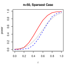
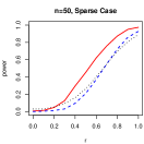
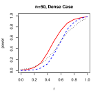
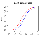
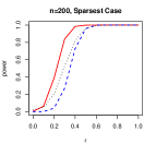
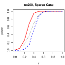
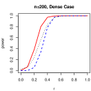
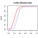
Figure 1: Empirical size ($r=0$) and power ($r>0$) of the proposed method (red-solid), the exponential scan method (blue-dashed) and the Fisher-type method (black-dotted) for the scalar-on-function family.

Function-on-function. The functional predictor $X$ is sampled as in the scalar-on-function case, while the noise process $Z$ is represented by

$$Z(t)=\sum_{j=1}^{k}\eta^{(j)}\phi_{j}(t)$$

for $k=50$, where $\phi_{1}(t)\equiv 1$, $\phi_{2j}(t)=\sqrt{2}\cos(2j\pi t)$ and $\phi_{2j+1}(t)=\sqrt{2}\sin(2j\pi t)$, and for each $j=1,\ldots,k$, $\eta^{(j)}$ is a random variable following the centered Laplacian distribution $\text{Laplace}(0,\sqrt{\lambda_{j}/2})$. Consequently, the process $Y$ is non-Gaussian.

For the slope operator, we consider $\beta(s,t)=rg(s,t)$ with $g(s,t)\in\mathbb{R}$ being one of the following:

• (Sparsest) $g(s,t)=\frac{5}{7}$;

• (Sparse) $g(s,t)=\sum_{k=1}^{3}\sum_{j=1}^{3}\frac{10}{4}\frac{\phi_{j}(s)\phi_{k}(t)}{(j+2)^{1.2}(k+2)^{1.2}}$;

• (Dense) $g(s,t)=\sum_{k=1}^{K}\sum_{j=1}^{K}\frac{9}{4}\frac{\phi_{j}(s)\phi_{k}(t)}{(j+2)^{1.2}(k+2)^{1.2}}$ with $K=100$;

• (Densest) $g(s,t)=\frac{10}{4}(st)^{2}\sqrt{e^{(s+t)/2}}$.

The dense case represents a challenging setting as $\beta$ contains a large number of relatively weaker spectral signals, in contrast with the sparse case in which the spectral signals of $\beta$ are stronger.

We compare the proposed method with the chi-squared test (Kokoszka et al., 2008). The chi-squared test is also based on functional principal component analysis, but unlike our method, it requires a delicate choice of the number of principal components, as the choice has a visible influence on the performance of the test. In our simulations, we take the leading $K=4$ principal components as in Kokoszka et al. (2008); we also tried various values for $K$ and found that overall $K=4$ yields the best results for the chi-squared test. According to the results shown in Figure 2, the proposed method has a much larger power when the signal is sparse and the sample size is small, and has a performance similar to that of the chi-squared test in other cases.

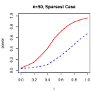
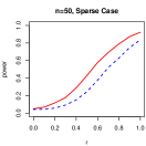
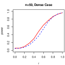
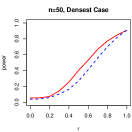
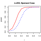
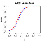
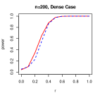
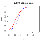
Figure 2: Empirical size ($r=0$) and power ($r>0$) of the proposed method (red-solid) and the chi-squared test (blue-dashed) for the function-on-function family.

Function-on-vector. The vector predictor $X\in\mathbb{R}^{q}$ with $q=5$ follows the centered multivariate Laplacian distribution with the covariance matrix $\Sigma=ADA^{\top}$ for $D=\text{diag}(\lambda_{1}\ldots,\lambda_{q})$, where $\lambda_{j}=j^{-1.5}$ and $A$ is an orthogonal matrix that is randomly generated and then remains fixed throughout the studies. The noise $Z$ is sampled as in the function-on-function case.

For the slope operator, we set $\beta(t)=rg(t)$ with $g(t)\in\mathbb{R}^{q}$, where for each $j=1,\ldots,q$, the $j$th component $g^{j}(t)$ of $g(t)$ is one of the following:

• (Sparest) $g^{j}(t)=\frac{11}{10}$;

• (Sparse) $g^{j}(t)=\sum_{k=1}^{3}\sum_{j=1}^{3}\frac{11}{4}\frac{\phi_{j}(\frac{j-1}{q-1})\phi_{k}(t)}{(j+2)^{1.2}(k+2)^{1.2}}$;

• (Dense) $g^{j}(t)=\sum_{k=1}^{K}\sum_{j=1}^{K}\frac{6}{4}\frac{\phi_{j}(\frac{j-1}{q-1})\phi_{k}(t)}{(j+2)^{1.2}(k+2)^{1.2}}$ with $K=100$;

• (Densest) $g^{j}(t)=\frac{11}{4}(\frac{j-1}{q-1})^{2}\sqrt{e^{\frac{j-1}{q-1}/4}}t^{2}\sqrt{e^{t/4}}$.

Similar to the function-on-function family, the dense case represents a more challenging setting for the proposed method. We compare the proposed method with the F-test developed by Zhang (2011). From the results shown in Figure 3, we observe that the proposed method is more powerful when the signal is relatively weak while the F-test has slightly higher power when the signal is strong.

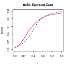
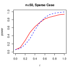
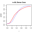
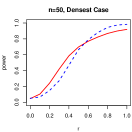
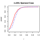
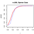
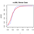
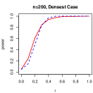
Figure 3: Empirical size ($r=0$) and power ($r>0$) of the proposed method (red-solid) and the F-test (blue-dashed) for the function-on-vector family.

5 Data Application

We apply the proposed method to study physical activities using data collected from wearable devices and available in the National Health and Nutrition Examination Survey (NHANES) 2005-2006. Over seven consecutive days, each participant wore a wearable device that for each minute recorded the average physical activity intensity level (ranging from 0 to 32767) in that minute. As the wearable devices were not waterproof, participants were advised to remove the devices when they swam or bathed. The devices were also removed when the participants were sleeping. For each subject, an activity trajectory, denoted by $A(t)$ for $t\in[0,7]$, was collected. In our study, trajectories with missing values or unreliable readings are excluded. To eliminate the effect of circadian rhythms that vary among participants, instead of the raw activity trajectories, we follow the practice in Chang and McKeague (2020+); Lin et al. (2022) to consider the activity profile $Y(s)=\mathrm{Leb}(\{t\in[0,7]:A(t)\geq s\})$ for $s=1,\ldots,32767$, where $\mathrm{Leb}$ denotes the Lebesgue measure on $\mathbb{R}$. The zero intensity values are also excluded since they may represent no activities like sleeping or intense activities like swimming. After these pre-processing steps, for the $i$th subject, we obtain an activity profile $Y_{i}(s)$ which is regarded as a densely observed function. Our goal is to study the effect of age on the activity profile. As children and adults, as well as males and females, have different activity patterns, we conduct the study on each group separately by using the proposed test, where the tuning parameter $\tau$ is selected by using the method of Lin et al. (2022).

First, we consider children with age from 6 to 17, including 6 and 17, and focus on the intensity spectrum $[1,1000]$ as children are found to have more moderate activities (WHO, 2020). As shown in Table 1, the age seems no impact on the activity profile for female children, but has significant impact for male children. By inspecting the mean activity profile curves in Figure 4, we see the visible differences for different age groups among male children, in contrast with the visually indistinguishable differences among female children. In particular, our test results and Fig. 4 together suggest that on average young male children tend to be significantly more active than elder male children.

Table 1: The p-values for testing the effect of age on the activity pattern, with sample size in the parentheses.

	Male	Female
p-value (age 6-17)	0.0046 (962)	0.1778 (952)
p-value (age 18-35)	0.1336 (623)	0.0282 (823)

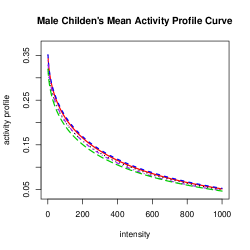
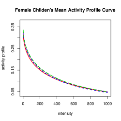
Figure 4: Mean activity profile curves among male children (left) and female children (right) for different age groups, namely, age 6-8 (red-solid), age 9-10 (blue-dashed), age 11-12 (black-dotted), 13-14 (purple-dash-dotted) and age 15-17 (green-dashed).

Now we consider the young adults with age from 18 to 35, and focus on the intensity spectrum $[1,3000]$. As shown in Table 1, there is significant difference of mean activity profiles among female young adults, while the difference is not significant among the males. This also agrees with the mean activity profiles shown in Fig. 5, where we observe significant difference in the mean activity profiles among different age groups of females, especially on the intensity spectrum $[300,1500]$, while the difference is less pronounced among males.

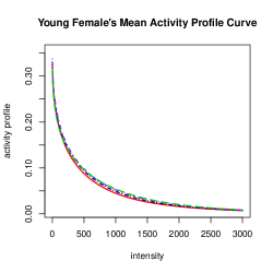
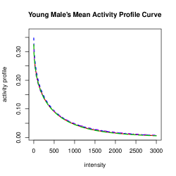
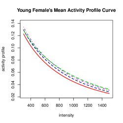
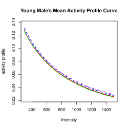
Figure 5: Mean activity profile curves among young female (top-left) and male (top-right) adults with their zoom-in regions (bottom) on the intensity spectrum $[300,1500]$ in different age groups, namely, age 18-21 (red-solid), age 22-25 (blue-dashed), age 26-29 (black-dotted), age 30-33 (purple-dash-dotted) and age 33-35 (green-dashed).

6 Concluding Remarks

In our theoretical analysis, we assume the overall number $p=p_{1}p_{2}$ of principal components to grow at a rate slower than $n$. This assumption is primarily used to ensure that the sequences ${V_{i}(\tilde{\phi},\tilde{\psi})}$ induced by $(\tilde{\phi},\tilde{\psi})\in\mathcal{F}_{p}$ share a common variance decay pattern (see Proposition LABEL:prop-struct-tilde-V in the supplementary material for details) and that the adopted empirical principal components are sufficiently close to their population versions in the sense of Proposition 3.4. Nonetheless, the simulation studies show that $p_{1}=n$ and $p_{2}=n$ still produce superior numerical results, suggesting possible relaxation of the assumption on $p$. Such relaxation, however, seems rather difficult and thus is left for future exploration, as it requires a finer analysis of the theoretical properties of high-order functional principal component analysis; such analysis itself is already highly challenging.

Supplementary material

Supplementary material contains proofs for the theoretical results of this paper, some auxiliary results used in the proofs and a concentration inequality for empirical eigenelements. (PDF)

See iFLR-supp

References

- Burdejova et al. (2017) Burdejova, P., Härdle, W., Kokoszka, P., and Xiong, Q. (2017), “Change point and trend analyses of annual expectile curves of tropical storms,” Econometrics and statistics, 1, 101–117.
- Cai et al. (2006) Cai, T. T., Hall, P., et al. (2006), “Prediction in functional linear regression,” The Annals of Statistics, 34, 2159–2179.
- Cai et al. (2018) Cai, T. T., Zhang, L., and Zhou, H. H. (2018), “Adaptive functional linear regression via functional principal component analysis and block thresholding,” Statistica Sinica, 28, 2455–2468.
- Cao et al. (2020) Cao, G., Wang, S., and Wang, L. (2020), “Estimation and inference for functional linear regression models with partially varying regression coefficients,” Stat, 9, e286.
- Cardot et al. (1999) Cardot, H., Ferraty, F., and Sarda, P. (1999), “Functional linear model,” Statistics & Probability Letters, 45, 11–22.
- Cardot et al. (2003) — (2003), “Spline estimators for the functional linear model,” Statistica Sinica, 13, 571–591.
- Chang and McKeague (2020+) Chang, H.-w. and McKeague, I. W. (2020+), “Nonparametric comparisons of activity profiles from wearable device data,” manuscript.
- Conway (2007) Conway, J. B. (2007), A Course in Functional Analysis, vol. 96, New York, NY: Springer New York, 2nd ed.
- Ferraty and Vieu (2006) Ferraty, F. and Vieu, P. (2006), Nonparametric Functional Data Analysis: Theory and Practice, New York: Springer-Verlag.
- Hall and Horowitz (2007) Hall, P. and Horowitz, J. L. (2007), “Methodology and convergence rates for functional linear regression,” The Annals of Statistics, 35, 70–91.
- Hilgert et al. (2013) Hilgert, N., Mas, A., and Verzelen, N. (2013), “Minimax adaptive tests for the functional linear model,” The Annals of Statistics, 41, 838–869.
- Horváth and Kokoszka (2012) Horváth, L. and Kokoszka, P. (2012), Inference for functional data with applications, Springer Series in Statistics, Springer.
- Hsing and Eubank (2015) Hsing, T. and Eubank, R. (2015), Theoretical Foundations of Functional Data Analysis, with an Introduction to Linear Operators, Wiley.
- James et al. (2009) James, G. M., Wang, J., and Zhu, J. (2009), “Functional linear regression that’s interpretable,” The Annals of Statistics, 37, 2083–2108.
- Kokoszka et al. (2008) Kokoszka, P., Maslova, I., Sojka, J., and Zhu, L. (2008), “Testing for lack of dependence in the functional linear model,” Canadian Journal of Statistics, 36, 207–222.
- Kokoszka and Reimherr (2017) Kokoszka, P. and Reimherr, M. (2017), Introduction to Functional Data Analysis, Chapman and Hall/CRC.
- Kong et al. (2016) Kong, D., Xue, K., Yao, F., and Zhang, H. H. (2016), “Partially functional linear regression in high dimensions,” Biometrika, 103, 147–159.
- Lai et al. (2021) Lai, T., Zhang, Z., and Wang, Y. (2021), “Testing independence and goodness-of-fit jointly for functional linear models,” Journal of the Korean Statistical Society, 50, 380–402.
- Lei (2014) Lei, J. (2014), “Adaptive Global Testing for Functional Linear Models,” Journal of the American Statistical Association, 109, 624–634.
- Lin et al. (2017) Lin, Z., Cao, J., Wang, L., and Wang, H. (2017), “Locally Sparse Estimator for Functional Linear Regression Models,” Journal of Computational and Graphical Statistics, 26, 306–318.
- Lin et al. (2022) Lin, Z., Lopes, M. E., and Müller, H.-G. (2022), “High-dimensional MANOVA via Bootstrapping and its Application to Functional Data and Sparse Count Data,” Journal of the American Statistical Association, to appear.
- Lopes et al. (2020) Lopes, M. E., Lin, Z., and Müller, H.-G. (2020), “Bootstrapping max statistics in high dimensions: Near-parametric rates under weak variance decay and application to functional data analysis,” The Annals of Statistics, 48, 1214–1229.
- Lopes and Yao (2022) Lopes, M. E. and Yao, J. (2022), “A sharp lower-tail bound for Gaussian maxima with application to bootstrap methods in high dimensions,” Electronic Journal of Statistics, 16, 58–83.
- Müller et al. (2011) Müller, H.-G., Sen, R., and Stadtmüller, U. (2011), “Functional data analysis for volatility,” Journal of Econometrics, 165, 233–245.
- Qu and Wang (2017) Qu, S. and Wang, X. (2017), “Optimal Global Test for Functional Regression,” arxiv.
- Ramsay and Silverman (2005) Ramsay, J. O. and Silverman, B. W. (2005), Functional Data Analysis, Springer Series in Statistics, New York: Springer, 2nd ed.
- Ritter et al. (1995) Ritter, K., Wasilkowski, G. W., Wozniakowski, H., et al. (1995), “Multivariate integration and approximation for random fields satisfying Sacks-Ylvisaker conditions,” Annals of Applied Probability, 5, 518–540.
- Shang (2017) Shang, H. L. (2017), “Functional time series forecasting with dynamic updating: An application to intraday particulate matter concentration,” Econometrics and statistics, 1, 184–200.
- Shen and Faraway (2004) Shen, Q. and Faraway, J. (2004), “An F test for linear models with functional responses,” Statistica Sinica, 14, 1239–1257.
- Shin (2009) Shin, H. (2009), “Partial functional linear regression,” Journal of Statistical Planning and Inference, 139, 3405–3418.
- Smaga (2019) Smaga, Ł. (2019), “General linear hypothesis testing in functional response model,” Communications in Statistics-Theory and Methods, 1–16.
- Tang and Shi (2021) Tang, C. and Shi, Y. (2021), “Forecasting High-Dimensional Financial Functional Time Series: An Application to Constituent Stocks in Dow Jones Index,” Journal of Risk and Financial Management, 14, 343.
- Vershynin (2018) Vershynin, R. (2018), High-dimensional probability: An introduction with applications in data science, vol. 47, Cambridge university press.
- Wang et al. (2020) Wang, D., Zhao, Z., Yu, Y., and Willett, R. (2020), “Functional Linear Regression with Mixed Predictors,” arXiv preprint arXiv:2012.00460.
- WHO (2020) WHO (2020), “WHO Physical activity Fact Sheet,” https://www.who.int/news-room/fact-sheets/detail/physical-activity.
- Xue and Yao (2021) Xue, K. and Yao, F. (2021), “Hypothesis testing in large-scale functional linear regression,” Statistica Sinica, 31, 1101–1123.
- Yao et al. (2005) Yao, F., Müller, H.-G., and Wang, J.-L. (2005), “Functional linear regression analysis for longitudinal data,” The Annals of Statistics, 33, 2873–2903.
- Yuan and Cai (2010) Yuan, M. and Cai, T. T. (2010), “A reproducing kernel Hilbert space approach to functional linear regression,” The Annals of Statistics, 38, 3412–3444.
- Yuan et al. (2010) Yuan, M., Cai, T. T., et al. (2010), “A reproducing kernel Hilbert space approach to functional linear regression,” The Annals of Statistics, 38, 3412–3444.
- Zhang (2011) Zhang, J.-T. (2011), “Statistical inferences for linear models with functional responses,” Statistica Sinica, 21, 1431–1451.
- Zhang (2013) — (2013), Analysis of variance for functional data, London: Chapman & Hall.
- Zhou et al. (2013) Zhou, J., Wang, N.-Y., and Wang, N. (2013), “Functional Linear Model with Zero-value Coefficient Function at Sub-regions,” Statistica Sinica, 23, 25–50.
- Zhu et al. (2012) Zhu, H., Li, R., and Kong, L. (2012), “Multivariate varying coefficient model for functional responses,” The Annals of Statistics, 40, 2634–2666.