Applying explicit symplectic integrator to study chaos of charged particles around magnetized Kerr black hole

Abstract

In a recent work of Wu, Wang, Sun and Liu, a second-order explicit symplectic integrator was proposed for the integrable Kerr spacetime geometry. It is still suited for simulating the nonintegrable dynamics of charged particles moving around the Kerr black hole embedded in an external magnetic field. Its successful construction is due to the contribution of a time transformation. The algorithm exhibits a good long-term numerical performance in stable Hamiltonian errors and computational efficiency. As its application, the dynamics of order and chaos of charged particles is surveyed. In some circumstances, an increase of the dragging effects of the spacetime seems to weaken the extent of chaos from the global phase-space structure on Poincaré sections. However, an increase of the magnetic parameter strengthens the chaotic properties. On the other hand, fast Lyapunov indicators show that there is no universal rule for the dependence of the transition between different dynamical regimes on the black hole spin. The dragging effects of the spacetime do not always weaken the extent of chaos from a local point of view.

1 Introduction

The Kerr spacetime [1] as well as the Schwarzschild spacetime is integrable because the Carter constant [2] appears as a fourth constant of motion. However, a test charge motion in a magnetic field around the Kerr black hole or the Schwarzschild black hole is nonintegrable due to the absence of the fourth constant of motion. In some cases, the electromagnetic perturbation induces the onset of chaos and islands of regularity [3-10]. In particular, Takahashi $\&$ Koyama [11] found the connection between chaoticness of the motion and the black hole spin. That is, the chaotic properties are weakened with an increase of the black hole spin.

It is worth pointing out that the detection of the chaotical behavior needs reliable results on the trajectories. Usually, it needs long-time calculations, especially in the case of the computation of Lyapunov exponents. Thus, the adopted computational scheme is required to have good stability, high precision and small cost of computational time. Because these general relativistic curved spacetimes correspond to Hamiltonian systems with the symplectic nature, a low order symplectic integration scheme which respects the symplectic nature of Hamiltonian dynamics [12-14] is naturally regarded to as the most appropriate solver. The Hamiltonian systems for these curved spacetimes are not separable to the phase-space variables, therefore, no explicit symplectic integrators but implicit (or implicit and explicit combined) symplectic integrators [15-22] can be available in general. However, the implicit methods are more computationally demanding than the explicit ones at same order. To solve this problem, Wang et al. [23-25] split the Hamiltonians of Schwarzschild, Reissner-Nordström and Reissner-Nordström -(anti)-de Sitter spacetime geometries into four, five and six integrable separable parts, whose analytical solutions are explicit functions of proper time. In this way, explicit symplectic integrators were designed for the spacetime geometries. Unfortunately, the dragging effects of the spacetime by a rotating black hole make the Hamiltonian of Kerr spacetime have no desired splitting form similar to the Hamiltonian splitting form of Schwarzschild spacetime, and then lead to the difficulty in the construction of explicit symplectic integrators. This obstacle was successfully overcame by the introduction of time transformations of Mikkola [26] to the Hamiltonian of Kerr spacetime geometry. The obtained time-transformed Hamiltonian exists a desired splitting, and explicit symplectic integrators were established by Wu et al. [27]. At this point, a note is worthwhile on such time-transformed explicit symplectic integrators. They are constant time-steps in the new coordinate time and the algorithmic symplecticity can be maintained. Although they are variant time-steps in the proper coordinate time, the varying proper time-steps have only small differences and are approximately constant when the new integration time is not very long. In other words, the time transformation plays a main role in obtaining separable time-transformed Hamiltonian for the use of explicit symplectic integrators rather than adaptive time step control.

One of the main purposes in this paper is to explore whether the proposed explicit symplectic integrators for the Kerr spacetime geometry work well in the simulation of the chaotic motion of charged particles near the Kerr black hole immersed in a weak, asymptotically uniform external magnetic field. As another important purpose, we apply the established second-order explicit symplectic method to check the result of Takahashi $\&$ Koyama [11] on the dragging effects weakening the chaotic properties, and to survey how a small change of the magnetic parameter affects a dynamical transition from order to chaos. Besides the Poincaré map method, the methods of Lyapunov exponents [28, 29] and fast Lyapunov indicators [30-32] are employed to distinguish between regular and chaotic orbits and to quantify the dependence of transition from regular to chaotic dynamics on a certain parameter.

For the sake of our purposes, we introduce a Hamiltonian system for the description of charged particles moving around the Kerr black hole surrounded with an external magnetic field in Sect. 2. A second-order time-transformed explicit symplectic algorithm is constructed and used to quantify the transition from regular to chaotic dynamics by means of different methods finding chaos in Sect. 3. Finally, the main results are concluded in Sect. 4.

2 Kerr black hole with external magnetic field

Let us consider a particle with charge $q$ moving around the Kerr black hole, surrounded by an external asymptotically uniform magnetic field with strength $B$. The particle motion is described by the following Hamiltonian formalism [33]

$$H=\frac{1}{2}g^{\mu\nu}(p_{\mu}-qA_{\mu})(p_{\nu}-qA_{\nu}).$$ (1)

Contravariant Kerr metric $g^{\mu\nu}$ has nonzero components

$$g^{tt}=-\frac{D}{\Lambda\Sigma},~{}~{}g^{t\phi}=-\frac{2ar}{\Lambda\Sigma}=g^{\phi t},$$

$$g^{rr}=\frac{\Lambda}{\Sigma},~{}~{}~{}~{}~{}~{}g^{\theta\theta}=\frac{1}{\Sigma},$$

$$g^{\phi\phi}=\frac{\Sigma-2r}{\Lambda\Sigma\sin^{2}\theta};$$

$$\Sigma=r^{2}+a^{2}\cos^{2}\theta,~{}~{}~{}~{}\Lambda=r^{2}+a^{2}-2r,$$

$$D=(r^{2}+a^{2})^{2}-\Lambda a^{2}\sin^{2}\theta.$$

$A^{\mu}$ is an electromagnetic four-vector potential [33, 34]

$$A^{\mu}=aB\xi^{\mu}_{(t)}+\frac{B}{2}\xi^{\mu}_{(\phi)},$$ (2)

where $\xi^{\mu}_{(t)}=(1,0,0,0)$ and $\xi^{\mu}_{(\phi)}=(0,0,0,1)$ are timelike and spacelike axial Killing vectors. Obviously, the four-vector potential has two nonzero covariant components

$$A_{t} = aBg_{tt}+\frac{B}{2}g_{t\phi},$$ (3)

$$= -aB[1+\frac{r}{\Sigma}(\sin^{2}\theta-2)]$$

$$A_{\phi} = aBg_{t\phi}+\frac{B}{2}g_{\phi\phi}$$ (4)

$$= B\sin^{2}\theta[\frac{r^{2}+a^{2}}{2}+\frac{a^{2}r}{\Sigma}(\sin^{2}\theta-2)].$$

The above covariant metric’s components are

$$g_{tt}=-(1-\frac{2r}{\Sigma}),~{}~{}g_{t\phi}=-\frac{2ar\sin^{2}\theta}{\Sigma}=g_{\phi t},$$

$$g_{\phi\phi}=(r^{2}+a^{2}+\frac{2ra^{2}}{\Sigma}\sin^{2}\theta)\sin^{2}\theta.$$

$p_{\mu}$ represents a covariant generalized four-momentum, determined by the relation

$$\dot{x}^{\mu}=\frac{\partial H}{\partial p_{\mu}}=g^{\mu\nu}(p_{\nu}-qA_{\nu}).$$ (5)

Note that $\dot{x}^{\mu}$ is a derivative of coordinate $x^{\mu}=(t,r,\theta,\phi)$ with respect to proper time $\tau$, called as a 4-velocity. Eq. (5) is rewritten as

$$p_{\mu}=g_{\mu\nu}\dot{x}^{\nu}+qA_{\mu}.$$ (6)

Because $\dot{p}_{\mu}=-\partial H/\partial x^{\mu}$, $p_{t}$ and $p_{\phi}$ are constants of motion. They are the particle’s energy and angular momentum:

$$-E = p_{t}=g_{tt}\dot{t}+g_{t\phi}\dot{\phi}+qA_{t},$$ (7)

$$L = p_{\phi}=g_{t\phi}\dot{t}+g_{\phi\phi}\dot{\phi}+qA_{\phi}.$$ (8)

They have equivalent expressions

$$\dot{t} = -f_{1}(E+qA_{t})-f_{2}(L-qA_{\phi}),$$ (9)

$$\dot{\phi} = f_{2}(E+qA_{t})+f_{3}(L-qA_{\phi}),$$ (10)

where

$$f_{1} = \frac{g_{\phi\phi}}{g_{tt}g_{\phi\phi}-g^{2}_{t\phi}},$$ (11)

$$f_{2} = \frac{g_{t\phi}}{g_{tt}g_{\phi\phi}-g^{2}_{t\phi}},$$ (12)

$$f_{3} = \frac{g_{tt}}{g_{tt}g_{\phi\phi}-g^{2}_{t\phi}}.$$ (13)

Now, Eq. (1) is rewritten as

$$H = \frac{1}{2}g^{\mu\nu}(p_{\mu}-qA_{\mu})(p_{\nu}-qA_{\nu})$$ (14)

$$= F+\frac{1}{2}\frac{\Lambda}{\Sigma}p^{2}_{r}+\frac{1}{2}\frac{p^{2}_{\theta}}{\Sigma},$$

where $F$ is a function of $r$ and $\theta$ as follows:

$$F = \frac{1}{2}[g^{tt}(E+qA_{t})^{2}+g^{\phi\phi}(L-qA_{\phi})^{2}]$$ (15)

$$-g^{t\phi}(E+qA_{t})(L-qA_{\phi})$$

$$= \frac{1}{2}[f_{1}(E+qA_{t})^{2}+f_{3}(L-qA_{\phi})^{2}]$$

$$+f_{2}(E+qA_{t})(L-qA_{\phi})$$

$$= -\frac{D}{2\Lambda\Sigma}(E+qA_{t})^{2}+\frac{\Sigma-2r}{2\Lambda\Sigma\sin^{2}\theta}(L-qA_{\phi})^{2}$$

$$+\frac{2ar}{\Lambda\Sigma}(E+qA_{t})(L-qA_{\phi}).$$

In Eq. (14), we take the speed of light $c$ and the gravitational constant $G$ as geometrized units, $c=G=1$. The black hole’s mass $M$ is also one unit, $M=1$. In practice, dimensionless operations are given to the related quantities via a series of scale transformations. That is, $r\rightarrow rM$, $t\rightarrow tM$, $\tau\rightarrow\tau M$, $a\rightarrow aM$, $E\rightarrow Em$, $p_{r}\rightarrow mp_{r}$, $L\rightarrow mML$, $p_{\theta}\rightarrow mMp_{\theta}$, $q\rightarrow mq$, $B\rightarrow B/M$ and $H\rightarrow m^{2}H$, where $m$ denotes the particle’s mass. Hereafter, we take $\beta=qB$. For any rotating black hole in general relativity, its spin angular momentum always satisfies $|a|\leq 1$.

Because the timelike 4-velocity (5) always satisfies the relation $\dot{x}^{\mu}\dot{x}_{\mu}=-1$, the Hamiltonian (14) itself is identical to a given constant

$$H=-\frac{1}{2}.$$ (16)

Besides this value and $E$ and $L$, other constants do not exist in the system. Thus, the Hamiltonian is non-integrable.

3 Numerical investigations

Following the work of Wu et al. [27], we establish a second-order explicit symplectic integrator for a time-transformed Hamiltonian of the system (14). For comparison, a second-order implicit and explicit mixed symplectic method is applied to solve the Hamiltonian (14) in Sect. 3.1. Then, the explicit symplectic integrator is used to investigate the dependence of the regular and chaotic dynamics of the time-transformed Hamiltonian on a certain parameter by means of several methods finding chaos in Sect. 3.2.

3.1 Numerical integration scheme

Clearly, the Hamiltonian (14) is inseparable to the variables. Implicit symplectic methods can be applied to it without doubt. The first term $F$ in Eq. (14) is solved analytically, and the sum of the second and third terms is solved numerically by the second-order implicit midpoint symplectic method IM2 [15]. The explicit and implicit solutions compose a second-order implicit and explicit mixed symplectic integrator for $H$, labeled as IE2. Such a mixed integrators was discussed by several authors [17-22]. It can save labour compared with the midpoint rule IM2 directly acting on the whole Hamiltonian $H$.

On the other hand, Wu et al. [27] used a time transformation function

$$d\tau=g(r,\theta)dw,~{}~{}g(r,\theta)=\frac{\Sigma}{r^{2}}$$ (17)

to obtain a time-transformed Hamiltonian to the Kerr geometry. The time-transformed Hamiltonian can be solved by explicit symplectic integrators. In the present problem, the time-transformed Hamiltonian is

$$K=g(H+p_{0})=\frac{\Sigma}{r^{2}}(F+p_{0})+\frac{\Lambda}{2r^{2}}p^{2}_{r}+\frac{1}{2r^{2}}p^{2}_{\theta}.$$ (18)

$p_{0}=-H=1/2$ is a momentum with respect to coordinate $q_{0}=\tau$. Thus, $K$ is always identical to zero, $K=0$. The time-transformed Hamiltonian is split into five parts

$$K=K_{1}+K_{2}+K_{3}+K_{4}+K_{5},$$ (19)

where the sub-Hamiltonians read

$$K_{1} = \frac{\Sigma}{r^{2}}(F+p_{0}),$$ (20)

$$K_{2} = \frac{1}{2}p^{2}_{r},$$ (21)

$$K_{3} = -\frac{1}{r}p^{2}_{r},$$ (22)

$$K_{4} = \frac{a^{2}}{2r^{2}}p^{2}_{r},$$ (23)

$$K_{5} = \frac{1}{2r^{2}}p^{2}_{\theta}.$$ (24)

$K_{1}$ seems to be the same as that of Wu et al. [27] from the expressional form, but is unlike that of Wu et al. $K_{2}$, $K_{3}$, $K_{4}$ and $K_{5}$ are the same as those of Wu et al. The five sub-Hamiltonians have analytical solutions that are explicit functions of the new coordinate time $w$. Their solutions correspond to operators $\widetilde{K}_{1}$, $\widetilde{K}_{2}$, $\widetilde{K}_{3}$, $\widetilde{K}_{4}$ and $\widetilde{K}_{5}$. According to the idea of Wu et al., these operators can compose second-order explicit symplectic integrator for $K$:

$$S2(h) = \widetilde{K}_{5}(\frac{h}{2})\circ\widetilde{K}_{4}(\frac{h}{2})\circ\widetilde{K}_{3}(\frac{h}{2})\circ\widetilde{K}_{2}(\frac{h}{2})\circ\widetilde{K}_{1}(h)$$ (25)

$$\circ\widetilde{K}_{2}(\frac{h}{2})\circ\widetilde{K}_{3}(\frac{h}{2})\circ\widetilde{K}_{4}(\frac{h}{2})\circ\widetilde{K}_{5}(\frac{h}{2}),$$

where $h$ represents a new coordinate time-step. The use of fixed new coordinate time-step maintains the symplecticity of the algorithms for the time-transformed Hamiltonian $K$. However, the proper time $\tau$ takes varying step-sizes. Such symplectic integrators are adaptive time-steps [26, 35, 36]. However, the adaptive proper time step control is almost absent in the present problem because the time transformation function $1<g\leq 1+1/r^{2}\approx 1$ for $r\gg 1$. This indicates that the time transformation function mainly provides the desirable separable time-transformed Hamiltonian.

Based on the numerical results of Wu et al., the second-order explicit symplectic method S2 performs good computational efficiency and stabilizing error behavior, compared with the fourth-order explicit symplectic method S4. Thus, we focus on the application of S2 to the system (19). For comparison, the second-order implicit and explicit mixed symplectic integrator IE2 is applied to $H$. Let us take the time-step $h=1$. Note that $h=1$ denotes a proper time-step for IE2 and a new coordinate time-step for S2. The parameters are given by $E=0.995$, $L=4.6$, $a=0.5$ and $\beta=0.001$. The initial conditions are $\theta=\pi/2$ and $p_{r}=0$. The initial separations $r_{0}=11$ and 75 are respectively given to Orbits 1 and 2. The initial value of $p_{\theta}>0$ is determined by Eqs. (14) and (16). It is shown in Fig. 1(a) that Hamiltonian errors $\Delta=K$ for the explicit symplectic algorithm S2 and $\Delta=-H-1/2$ for the second-order implicit and explicit mixed symplectic method IE2 remain stable and bounded. Both algorithms give no explicit error differences to the same orbit. The errors have the same order for the two orbits. If IE2 is applied to $K$, the results are almost the same as those for the application of IE2 to $H$. Although S2 is not explicitly better than IE2 in numerical accuracy, it is in computational efficiency, as claimed in the work of Wu et al.

It is worth pointing out that IE2 and S2 work in different time systems. The integration time for IE2 is the proper time $\tau=10^{8}$. However, the integration time for S2 is the new coordinate time $w=10^{8}$. The new coordinate time $w=10^{8}$ and its corresponding real proper time have no large differences. This result is shown clearly in Table 1. In fact, differences between the solutions of $H$ and those of $K$ are negligible before the integration time arrives at $10^{5}$. So are the differences between the proper times of $K$ and the coordinate times of $K$. These facts confirm that the time transformation does not provide adaptive time-steps but a separable time-transformed Hamiltonian. Of course, these differences between the solutions of the two systems get slowly large as the integration time spans $10^{5}$ and increases. In this case, the solutions of $K$ at a given proper time are obtained with the aid of some interpolation method.

In fact, the tested orbits have different dynamical behaviors, as shown on Poincaré sections at the plane $\theta=\pi/2$ and $p_{\theta}>0$ in Fig. 1(b). The phase-space structure of Orbit 1 is a torus, regarded as the characteristic of an ordered orbit. However, the phase-space structure of Orbit 2 has many discrete points that are randomly filled in an area, regarded as the characteristic of a chaotic orbit. It can be seen from Fig. 1(a) that the performance of S2 (with IE2) is independent of the regularity and chaoticity of orbits. The phase-space structures in Fig. 1(b) are described by S2. They are also given by IE2.

3.2 Dynamical transition with parameters varying

In what follows, we use the algorithm S2 to trace the orbital dynamics of the system $K$. Meantime, methods of Poincaré sections, Lyapunov exponents and fast Lyapunov indicators are employed to find chaos.

3.2.1 Poincaré sections

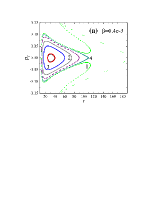
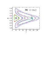
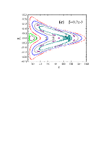
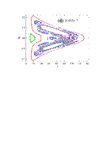
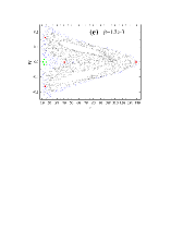
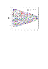
Figure 2: Same as Fig. 1(b), but for different values of the magnetic parameter $\beta$. An increase of $\beta$ results in strengthening the extent of chaos. Orbit 3 with the initial separation $r_{0}=60$ in panel (d) is weakly chaotic.

It is worth pointing out that the chaoticity of Orbit 2 is due to the charged particle suffered from the electromagnetic field interaction. As claimed in the Introduction, the Kerr spacetime without the electromagnetic field interaction holds the Carter constant as the fourth integral of motion and therefore is integrable and nonchaotic. If the electromagnetic field is included in the Kerr spacetime, then the Carter constant is no longer present and the dynamics of charged particles becomes nonintegrable. This nonintegrability is an insufficient but necessary condition for the occurrence of chaos. When the electromagnetic field interaction acts as a relatively small perturbation, the gravitational force from the black hole is a dominant force and the dynamical system is nearly integrable. In this case, the Kerr spacetime with the electromagnetic field interaction can exhibit the similar dynamical features of the Kerr spacetime without the electromagnetic field interaction. That is to say, no chaos occurs and all orbits are regular Kolmogorov-Arnold-Moser (KAM) tori. This result is suitable for the magnetic parameter $\beta=4\times 10^{-4}$ in Fig. 2(a). The tori in the perturbed case unlike those in the unperturbed case are twisted in the shapes; e.g., Orbit 1 corresponds to a peculiar torus, and Orbit 4 with initial separation $r_{0}=110$ yields a triangle torus. When $\beta=6\times 10^{-4}$ in Fig. 2(b), the tori are still present, but are to a large degree different from those for $\beta=4\times 10^{-4}$ in the shapes. There are typical differences of Orbits 1, 2 and 3 between Figs. 2 (a) and (b). In particular, Orbit 4 in Fig. 2(a) is evolved to a twisted figure-eight orbit with a hyperbolic point in Fig. 2(b) due to the electromagnetic field interaction. Such a hyperbolic point has a stable direction and another unstable direction, and easily induces chaos. As the electromagnetic field interaction increases and can generally match with the black hole gravitational force, chaos occurs. The hyperbolic point causes Orbit 4 to be chaotic for $\beta=7\times 10^{-4}$ in Fig. 2(c). When the magnetic field strength is further enhanced, e.g., $\beta=8\times 10^{-4}$ in Fig. 2(d), $\beta=1\times 10^{-3}$ in Fig. 1(b) and $\beta=1.2\times 10^{-3}$ in Fig. 2(e), chaos becomes stronger and stronger. Particular for $\beta=3\times 10^{-3}$ in Fig. 2(f), chaos is existent almost everywhere in the whole phase space. In a word, it can be concluded clearly from Figs. 1(b) and 2 that an increase of the magnetic parameter is easier to induce chaos and enhances the strength of chaos from the global phase-space structure.

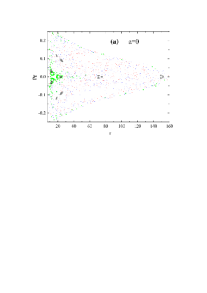
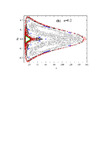
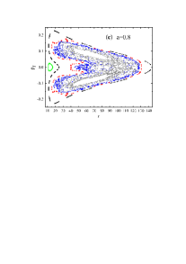
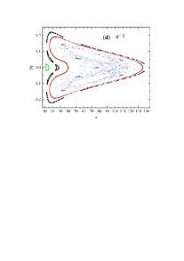
Figure 3: Same as Fig. 1(b), but for different values of the black hole’s angular momentum $a$. Here, the magnetic parameter $\beta=1\times 10^{-3}$. An increase of $a$ seems to weaken the extent of chaos from the global phase space structure.

On the other hand, we are also interested in knowing what the dynamical transition with an increase of the black hole angular momentum $a$ is. To answer this question, we consider some values of $a$. For $a=0$ corresponding to the Schwarzschild case in Fig. 3(a), chaos densely exists almost everywhere in the whole phase space. This does not mean that any regular orbits are ruled out. In fact, regular Orbit 2 and black orbit with initial separation $r_{0}=25$ in Fig. 1(b) are still ordered in Fig. 3(a). Given $a=0.2$, chaotic Orbits 1 and 3 in Fig. 3(a) become regular in Fig. 3(b), whereas ordered Orbit 2 in Fig. 3(a) becomes chaotic in Fig. 3(b). As the spin frequently increases [e.g., $a=0.5$ in Fig. 1(b), $a=0.8$ in Fig. 3(c) and $a=1$ in Fig. 3(d)], the regular region seems to gradually increase and the chaotic region seems to decrease. In other words, an increase of $a$ seems to weaken the extent of chaos from the global phase-space structure. This seems to support the result of [11] about the black hole spin weakening the chaotic properties. However, this does not mean that some individual orbits must be more chaotic as the dragging effects of the spacetime by a rotating black hole decrease. For example, Orbit 2 is regular for $a$=0, 1 but chaotic for $a$=0.2, 0.5, 0.8.

3.2.2 Fast Lyapunov indicators

Apart from the Poincaré map method, the technique of Lyapunov exponents is very efficient to detect the onset of chaos and provides a quantitative measure to chaos. An average exponential deviation of two nearby orbits in the system $K$ is measured by the largest Lyapunov exponent

$$\lambda=\lim_{w\rightarrow\infty}\frac{1}{w}\ln\frac{d(w)}{d(0)},$$ (26)

where $d(0)$ and $d(w)$ represent the separations between the two nearby orbits at times 0 and $w$, respectively. Precisely speaking, $d(w)$ is written as

$$d(w) = [(r_{2}-r_{1})^{2}+(\theta_{2}-\theta_{1})^{2}+(p_{r2}-p_{r1})^{2}$$ (27)

$$+(p_{\theta 2}-p_{\theta 1})^{2}]^{1/2},$$

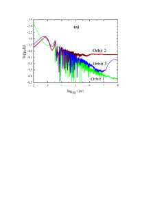
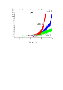
Figure 4: (a) Lyapunov exponents of three orbits including Orbits 1 and 2 in Fig. 1 and Orbit 3 in Fig. 2(d). The Lyapunov exponent (colored red) of Orbit 2 calculated in the new coordinate time $w$ coincides with that (colored black) of Orbit 2 computed in the proper time $\tau$. Orbit 1 is regular, whereas Orbits 2 and 3 show the onset of chaos. (b) Fast Lyapunov indicators (FLIs) of the three orbits. The FLI of Orbit 2 reaches 12 when the integration time $w=6\times 10^{5}$, but is larger than 200 for the integration time $w=10^{7}$. Thus, this orbit is strongly chaotic. Weak chaos of Orbit 3 can be distinguished from regular Orbit 1 in terms of the growth of FLIs of the two orbits during the integration time $w=10^{7}$.

where $(r_{1},\theta_{1},p_{r1},p_{\theta 1})$ is a set of phase-space variables of one orbit at time $w$ and $(r_{2},\theta_{2},p_{r2},p_{\theta 2})$ is a set of phase-space variables of its nearby orbit. Three points should be noted. (i) The initial distance $d(0)$ had better be $10^{-8}$ in the double-precision case. (ii) Appropriate renormalizations to the distance $d(w)$ are required from time to time. (iii) Although the Lyapunov exponent depends on the choice of spacetime coordinates, it is very approximate to an invariant Lyapunov exponent because the new coordinate time $w$ and its corresponding proper time $\tau$ are approximately equal, and the distance $d(w)$ and its corresponding proper distance are, too. More details about the invariant Lyapunov exponent were given by Wu $\&$ Huang [29] and Wu et al. [32]. A positive Lyapunov exponent indicates the chaoticity of a bounded orbit, and zero Lyapunov exponent describes the regularity of a bounded orbit. This allows us to detect chaos from order. It is clearly seen from the Lyapunov exponents in Fig. 4(a) that Orbits 1 and 2 in Fig. 1 are ordered and chaotic, respectively. Orbit 3 in Fig. 2(d) seems to be regular till $w=10^{7}$ because its Lyapunov exponent like Orbit 1’s Lyapunov exponent decreases and does not tend to a stabilizing value. However, the Lyapunov exponent of Orbit 3 unlike that of Orbit 1 tends to a stabilizing positive value when the integration time spans from $10^{7}$ to $10^{8}$; therefore, Orbit 3 is chaotic. Because the Lyapunov exponent of Orbit 3 is smaller than that of Orbit 2, the chaoticity of Orbit 3 is weaker than that of Orbit 2. The result is consistent with that described by the method of Poincaré sections in Figs. 1(b) and 2(d).

In general, a long enough integration time is necessary to obtain a stabilizing value of Lyapunov exponent. In particular, the chaoticity of Orbit 3 cannot be distinguished from the regularity of Orbit 1 in terms of Lyapunov exponents until $w=10^{8}$. Compared with the method of Lyapunov exponents, the fast Lyapunov indicator (FLI) of Froeschlé $\&$ Lega [31] is based on computations of tangent vectors and is regarded as a quicker technique to separate chaotic orbits from regular ones. Wu et al. [32] modified the FLI with tangent vectors as the FLI of two nearby orbits:

$$FLI=\log_{10}\frac{d(w)}{d(0)}.$$ (28)

Here, $d(0)=10^{-9}$ is admissible in the double-precision case, and a few but not many renormalizations to the distance $d(w)$ are still necessary to avoid the saturation of orbits. Regular and chaotic orbits can be identified according to completely different time rates of growth of FLIs. An exponential increase of FLI of a bounded with time $\log_{10}w$ indicates the chaoticity of the orbit; an algebraical increase of FLI of a bounded with time $\log_{10}w$ indicates the regularity of the orbit. In other words, if the FLI of a bounded orbit is much larger than that of another bounded orbit for a given time, the former orbit is chaotic, but the latter orbit is regular. On the basis of this point, the properties of orbits in Fig. 4(b) can be known easily. Without doubt, Orbit 2 is strongly chaotic because its FLI arrives at 12 when the integration time $w=6\times 10^{5}$, and is larger than 200 when $w=10^{7}$. Unlike the Lyapunov exponents, the FLIs are easy to distinguish between the regularity of Orbit 1 and the chaoticity of Orbit 3 when $w=10^{7}$ because the FLI of Orbit 1 is smaller than 6, but the FLI of Orbit 3 is 13.5.

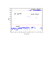
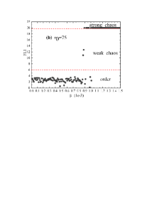
Figure 5: Dependence of the values of FLIs on the magnetic parameter $\beta$. The other parameters are $E=0.995$, $L=4.6$ and $a=0.5$. The initial conditions $\theta=\pi/2$ and $p_{r}=0$ are the same in the two panels, but the initial values $r_{0}$ and $p_{\theta}>0$ are different. For the strong chaotic case, the integration ends when the FLI reaches 20, whereas the integration time $w=10^{7}$ for the two other cases.

As claimed in Ref. [32], the FLI is a good tool to allow us to identify the transition between different dynamical regimes with a variation of a certain dynamical parameter. Letting $a=0.5$ be fixed and $\beta$ run from 0 to $1.5\times 10^{-3}$, we trace the dependence of the dynamical transition on the magnetic parameter. For a given value $\beta$, the integration lasts to the time $w=10^{7}$, but it ends if the FLI of some orbit is 20. There are three areas: regular area with FLIs smaller than 6, weak chaos area with FLIs no less than 6 but no more than 20 and strong chaos area with FLIs larger than 20. When $\beta<0.7\times 10^{-3}$, no chaos occurs in Figs. 5 (a) and (b). This is because the magnetic field force to charged particles is smaller than the black hole gravity to charged particles, as is mentioned above. $\beta<0.7\times 10^{-3}$ is a regular area of the magnetic parameter. Chaos will get easier to a large degree as $\beta$ increases. When $\beta>0.8\times 10^{-3}$, many values of $\beta$ correspond to the onset of chaos and many other values indicate the presence of order in Fig. 5(a). In particular, chaos and order are present in the neighbourhood of $\beta=1.5\times 10^{-3}$. Unlike in Fig. 5(a), all values of $\beta>1.1\times 10^{-3}$ can induce strong chaos in Fig. 5(b). Of course, few values of the magnetic parameter correspond to weak chaos in the two panels. In short, the technique of FLIs and the method of Poincaré sections consistently show that an increase of the magnetic parameter leads to a strong probability for inducing the occurrence of chaos and strengthening the extent of chaos.

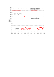
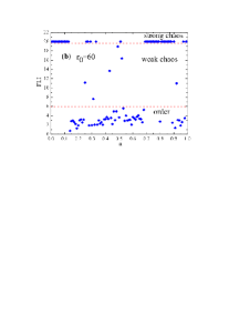
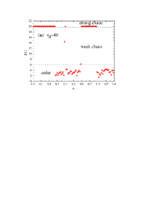
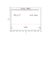
Figure 6: Same as Fig. 5, but the dependence of the values of FLIs on the black hole spin $a$. Here, $\beta=0.001$.

Figs. 6 (a)-(d) plot the dependence of FLIs on the black hole spin $a$ when $\beta=0.001$ is fixed. Strong chaos occurs as $a\rightarrow 0$ but no chaos appears as $a\rightarrow 1$ for the initial separation $r_{0}=40$ in Fig. 6(a). For the most values of $a\in[0.25,0.65]$, chaos is absent, too. The transition has some differences for the initial separation $r_{0}=60$ in Fig. 6(b). Chaos exists when $a\rightarrow 1$. However, there is no chaos at the left end $a=0$ and the right end $a=1$ in Figs. 6 (c) and (d). These facts show that different combinations of initial conditions and other dynamical parameters affect the dependence of the dynamical transition on the black hole spin. Thus, no universal rule can be given to the relation between the dynamical transition and the black hole spin.

A notable point is that the aforementioned results are completely based on mathematical calculations. To justify the mathematical correctness of the obtained results, we employ an eighth- and ninth-order Runge-Kutta-Fehlberg integrator (RKF89) with adaptive step sizes to integrate the system (14) or (19). This algorithm can provide a machine precision to the Hamiltonians if roundoff errors are ignored. Of course, the higher-order method is more expensive in computations than the second-order explicit scheme S2. Consequently, the results obtained from RKF89 are consistent with those given by S2. It is very perfect and idealized to make a comparison of the obtained theoretical results with real observational results in the relativistic astrophysics. However, the known observational results have not sufficiently supported the study of chaotic behavior of black holes. There are two main reasons. On one hand, it costs a long enough time span to distinguish between the regular and chaotic two cases. The time for the determination of chaos is $10^{7}M$ or $10^{8}M$ from the numerical computations. Nevertheless, it is impossibly available from the observations. On the other hand, it costs massive data to detect chaos from order. This fact can be seen clearly from the numerical simulations. However, only a small amount of observational data are given. Because of these reasons, the study of chaos and islands of regularity of black holes in all the known publications such as [3-11, 23-25, 33 and 34] is restricted to the theoretically numerical results rather than the real observational results.

4 Conclusion

Because of the dragging effects of the spacetime by a rotating black hole, the Kerr geometry is complicated. In spite of this, it is integrable and nonchaotic. When an external magnetic field is included, the dynamics of charged particles becomes more complicated. In fact, it is nonintegrable and possibly chaotic. We find that the second-order explicit symplectic integrator for the integrable Kerr spacetime proposed in the work of Wu et al. [27] is still suited for the present nonintegrable problem. The successful application of the explicit symplectic integrator is owing to the contribution of the time transformation given in Eq. (17). The theoretical analysis and numerical results show that such a time transformation does not mainly bring adaptive proper time steps but a separable time-transformed Hamiltonian, which satisfies a need for the use of explicit symplectic integrator. The explicit symplectic algorithm performs good performance in numerical accuracy, stable error behaviour and computational cost regardless of whether tested orbits are regular or chaotic.

The explicit symplectic integrator is very suitable for studying the long-term qualitative evolution of orbits of charged particles moving around the magnetized Kerr black hole. The electromagnetic force interactions are mainly responsible for the nonintegrability and chaoticity of charged particle dynamics. In some circumstances, charged particle motions can be chaotic. An increase of the dragging effects of the spacetime seems to weaken the extent of chaos from the global phase-space structure on Poincaré sections. However, an increase of the magnetic parameter results in strengthening the chaotic properties. On the other hand, the fast Lyapunov indicators by scanning the black hole spin parameter show that no universal rule can be given to the dependence of the transition between different dynamical regimes on the black hole spin. This is because the transition is dependent on not only the spin parameter but also different combinations of initial conditions and other parameters. Unlike an increase of the black hole spin, that of the magnetic parameter may much easily induce chaos.

Acknowledgements: The authors are very grateful to two referees for valuable comments and suggestions. This research has been supported by the National Natural Science Foundation of China [Grant Nos. 11973020 (C0035736), 11533004, 11803020, 41807437, U2031145], and the Natural Science Foundation of Guangxi (Grant Nos. 2019JJD110006 and 2018GXNSFGA281007).

Table 1: Solutions for the methods S2 and IE2 solving Orbit 1 in Fig. 1(a). The two systems $H$ and $K$ almost have the same solutions in an integration time of $\tau=10000$ or $w=10000$.

	$w$	$\tau$	$r$	$\theta$	$p_{r}$	$p_{\theta}$
$H$	/	1	11.0031	1.5867	7.6213e-3	1.9255
$K$	1	1	11.0031	1.5867	7.6203e-3	1.9255
$H$	/	10	11.3074	1.7235	7.3287e-2	1.7922
$K$	10	10.0002	11.3075	1.7235	7.3281e-2	1.7921
$H$	/	$10^{2}$	26.2463	1.9136	0.2041	-1.0078
$K$	$10^{2}$	100.0094	26.2473	1.9136	0.2041	-1.0079
$H$	/	$10^{3}$	126.4088	1.5798	6.3895e-2	-1.8227
$K$	$10^{3}$	1000.0118	126.3912	1.5797	6.3868e-2	-1.8226
$H$	/	$10^{4}$	132.8861	1.5449	-5.1566e-2	-3.0532
$K$	$10^{4}$	10000.1079	132.7308	1.5441	-5.1730e-2	-3.0572
$H$	/	$10^{5}$	37.3004	1.1427	-0.1763	-1.4168
$K$	$10^{5}$	100001.0807	33.7413	1.1251	-0.1827	-1.2180
$H$	/	$10^{6}$	150.9389	1.6606	1.2518e-2	-2.0503
$K$	$10^{6}$	1000011.0250	151.8362	1.6616	-2.7765e-3	-2.0940
$H$	/	$10^{7}$	142.0132	1.5745	-3.5099e-2	-3.0676
$K$	$10^{7}$	10000110.1522	110.0560	1.6668	8.0709e-2	-3.0845

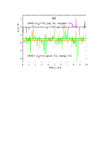
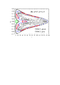
Figure 1: (a) Hamiltonian errors $\Delta=K$ for the explicit symplectic algorithm S2 and $\Delta=-H-1/2$ for the second-order implicit and explicit mixed symplectic method IE2. The parameters are $E=0.995$, $L=4.6$, $a=0.5$ and $\beta=0.001$. Orbits 1 and 2 have their initial separations $r_{0}=11$ and 75, respectively. The other initial conditions are $\theta=\pi/2$, $p_{r}=0$ and $p_{\theta}>0$ given by Eqs. (14) and (16). $h=1$ is a proper time step for IE2 and a new coordinate time step for S2. Both algorithms make the errors have no secular drift and remain of the same order for Orbits 1 and 2. (b) Poincaré sections on the plane $\theta=\pi/2$ and $p_{\theta}>0$, given by S2. It is clear that Orbit 1 is regular, whereas Orbit 2 is chaotic.

References

- Kerr (1963) R. P. Kerr, Phy. Rev. Lett. 11, 237 (1963)
- Carter (1968) B. Carter, Phy. Rev. 174, 1559 (1968)
- Nakamura & Ishizuka (1968) Y. Nakamura, T. Ishizuka, Astrophys. Space Science 210, 105 (1993)
- Kopáček et al. (2010) O. Kopáček, V. Karas, J. Kovář, Z. Stuchlík, Astrophys. J. 722, 1240 (2010)
- Kopáček & Karas (2014) O. Kopáček, V. Karas, Astrophys. J. 787, 117 (2014)
- Kopáček & Karas (2018) O. Kopáček, V. Karas, Astrophys. J. 853, 53 (2018)
- Frolov & Shoom (2010) V. P. Frolov, A. A. Shoom, Phys. Rev. D 82, 084034 (2010)
- Kopáček et al. (2017) M. Kološ, A. Tursunov, Z. Stuchlík, Eur. Phys. J. C 77, 860 (2017)
- Pánis et al. (2019) R. Pánis, M. Kološ, Z. Stuchlík, Eur. Phys. J. C 79, 479 (2019)
- Stuchlík et al. (2020) Z. Stuchlík, M. Kološ, J. Kovář, P. Slaný, A. Tursunov, Universe 6, 26 (2020)
- Takahashi & Koyama (2009) M. Takahashi, H. Koyama, Astrophys. J. 693, 472 (2009)
- Wisdom (1982) J. Wisdom, Astron. J. 87, 577 (1982)
- Ruth (1983) R. D. Ruth, IEEE Trans. Nucl. Sci. NS 30, 2669 (1983)
- Wisdom & Holman (1991) J. Wisdom J., M. Holman, Astron. J. 102, 1528 (1991)
- Feng (1986) K. Feng, Journal of Computational Mathematics 44, 279 (1986)
- Brown (2006) J. D. Brown, Phys. Rev. D 73, 024001 (2006)
- Liao (2006) X. H. Liao, Celest. Mech. Dyn. Astron. 66, 243 (1997)
- Preto (2009) M. Preto, P. Saha, Astrophys. J. 703, 1743 (2009)
- Lubich & Walther (2010) C. Lubich, B. Walther, B. Brügmann, Phys. Rev. D 81, 104025 (2010)
- Zhong et al. (2010) S. Y. Zhong, X. Wu, S. Q. Liu, X. F. Deng, Phys. Rev. D 82, 124040 (2010)
- Mei et al. (2013a) L. Mei, X. Wu, F. Liu, Eur. Phys. J. C 73, 2413 (2013)
- Mei et al. (2013b) L. Mei, M. Ju, X. Wu, S. Liu, Mon. Not. R. Astron. Soc. 435, 2246 (2013)
- Wang et al. (2021a) Y. Wang, W. Sun, F. Liu, X. Wu, Astrophys. J. 907, 66 (2021) (Paper I)
- Wang et al. (2021b) Y. Wang, W. Sun, F. Liu, X. Wu, Astrophys. J. 909, 22 (2021) (Paper II)
- Wang et al. (2021c) Y. Wang, W. Sun, F. Liu, X. Wu, Astrophys. J. Supp. Series 254, 8 (2021) (Paper III)
- Mikkola (1997) S. Mikkola, Celest. Mech. Dyn. Ast. 67, 145 (1997)
- Wu et al. (2021) X. Wu, Y. Wang, W. Sun, F. Liu, Astrophys. J. 914, 63 (2021) (Paper IV)
- Tancredi et al. (2001) G. Tancredi, A. Sánchez, F. Roig, Astron. J. 121, 1171 (2001)
- Wu & Huang (2003) X. Wu, T.-Y. Huang, Phys. Lett. A 313, 77 (2003)
- Froeschlé et al. (1997) C. Froeschlé, E. Lega, R. Gonczi, Celest. Mech. Dyn. Astron. 67, 41 (1997)
- Froeschlé & Lega (1997) C. Froeschlé, E. Lega, Celest. Mech. Dyn. Astron. 78, 167 (2000)
- Wu et al. (2006) X. Wu, T.-Y. Huang, H. Zhang, Phys. Rev. D 74, 083001 (2006)
- Stuchlík & Kološ (2016) Z. Stuchlík, M. Kološ, Eur. Phys. J. C 76, 32 (2016)
- Tursunov et al. (2016) A. Tursunov, Z. Stuchlík, M. Kološ, Phys. Rev D 93, 084012 (2016)
- Mikkola & Tanikawa (1999) S. Mikkola, K. Tanikawa, Celest. Mech. Dyn. Ast. 74, 287 (1999)
- Preto & Tremaine (1999) M. Preto, S. Tremaine, Astron. J. 118, 2532 (1999)