Postulating Exoplanetary Habitability via a Novel Anomaly Detection Method

Abstract

A profound shift in the study of cosmology came with the discovery of thousands of exoplanets and the possibility of the existence of billions of them in our Galaxy. The biggest goal in these searches is whether there are other life-harbouring planets. However, the question which of these detected planets are habitable, potentially-habitable, or maybe even inhabited, is still not answered. Some potentially habitable exoplanets have been hypothesized, but since Earth is the only known habitable planet, measures of habitability are necessarily determined with Earth as the reference. Several recent works introduced new habitability metrics based on optimization methods. Classification of potentially habitable exoplanets using supervised learning is another emerging area of study. However, both modeling and supervised learning approaches suffer from drawbacks. We propose an anomaly detection method, the Multi-Stage Memetic Algorithm (MSMA), to detect anomalies and extend it to an unsupervised clustering algorithm MSMVMCA to use it to detect potentially habitable exoplanets as anomalies. The algorithm is based on the postulate that Earth is an anomaly, with the possibility of existence of few other anomalies among thousands of data points. We describe an MSMA-based clustering approach with a novel distance function to detect habitable candidates as anomalies (including Earth). The results are cross-matched with the habitable exoplanet catalog (PHL-HEC) of the Planetary Habitability Laboratory (PHL) with both optimistic and conservative lists of potentially habitable exoplanets.

1 Introduction

Thousands of exoplanets have been discovered in last few decades, with implication that there are more planets than stars in our Galaxy. Ultimately, we are searching for habitable planets or, at least, for potentially habitable. By potentially habitable planets we understand those classes or types of planets whose properties indicate their ability to beget or sustain life, such as e.g. being a rocky planet in a habitable zone (HZ) of the host star allowing for a liquid water on the surface, and so on. By applying various Earth-based criteria, more than one potentially habitable exoplanets have indeed been hypothesized. The Habitable Exoplanets Catalog (HEC) maintained by the PHL describes a small fraction of all discovered planets as potentially habitable. These are divided into two categories: optimistic (24 planets) and conservative (36 planets) lists of potentially habitable exoplanets. Since the number of potentially habitable exoplanets is significantly less than the non-habitable ones, these habitable candidates could be thought of as anomalies in a large pool of normal (non-habitable) instances. The idea of equating the habitability detection problem to an anomaly detection problem therefore deserves merit, and no method supporting this hypothesis exists currently in the literature. The idea resonates well with the fact that Earth is the only known habitable planet among several thousand detected, and there is a possibility that life is arbitrarily rare (Spiegel and Turner, 2012). Backed by such physical observations, it is reasonable to postulate Earth as an anomaly, and hypothesize the potentially habitable planets as anomalies. This will allow the anomaly detection, i.e. habitable exoplanet detection problem, to be framed as an unsupervised machine learning (ML) approach via a novel clustering algorithm. Consequently, we can estimate the absolute prerequisites for habitability in order to set up a list of planets harbouring life indicators, using the examples from our own planet.

Our hypothesis is that this small fraction of planets are anomalous instances in a large pool of ‘non-habitable’ exoplanets (a total of 4383 planets are confirmed so far, with 5912 candidates). With this large number of discovered exoplanets, it is imperative to examine these rare instances by characterizing all exoplanets in terms of planetary parameters, types, populations and, ultimately, the habitability potential. This needs the knowledge of multiple planetary parameters from observations which, in turn, demands hours of expensive telescope time. Therefore, we need to prioritize the planets to examine, i.e. develop a quick screening tool for evaluating habitability perspectives from observed properties.

2 Habitability Quantification and Classification: Existing Approaches

Detecting potentially habitable exoplanets using machine learning tools have gained momentum in recent times (Bora et al., 2016; Saha et al., 2018; Basak et al., 2020). This research suggests that the habitability can be viewed as probabilistic measure (Bora et al., 2016), and such approaches require optimization and classification methods. Two popular approaches to habitability estimation are discussed below.

2.1 Metric-based quantification

Bora et al. (2016) introduced a Cobb-Douglas Habitability Score – a metric based on Cobb-Douglas habitability production function (CD-HPF), which computes the habitability score by using measured and estimated planetary parameters. Basak et al. (2020) extended the CDHS model and proposed another quantitative metric for habitability – CEESA, which considers orbital eccentricity in addition to the same features used by the CDHS. These metrics, based on optimization methods, use only four physical planetary parameters (mass, density, radius and surface temperature), while there may be a need to accommodate more features such as, for ex., eccentricity, or orbital separation. In Limbach et al. (2015) it was proposed that low eccentricity favours multiple planetary systems which, in turn, favours habitability as it may stabilize the climate on a planet (Wang et al., 2017). While it is acceptable to reason that many factors of life are dependent on temperature, habitability metrics should be assessed on more parameters than just the temperature. Factors such as escape velocity, eccentricity and many others, are important while determining whether a planet can be potentially habitable or not. For example, the brown dwarf WD 0806-661B has the surface temperature of $52^{\circ}-77^{\circ}$C (Luhman et al., 2011), which is in the habitable range (Earth average temperature is $\sim$15^∘C), but the planet has a mass of 7 to 9 $M_{\rm Jup}$ — too massive to be potentially habitable. Some researchers (e.g. Tasker et al. (2017)) even suggest that it is impossible to compare habitability on different planets quantitatively based on a single habitability score or metric.

2.2 Supervised learning

Saha et al. (2018) applied a statistical ML classification method (XGBoost), where the training data with multiple features are used to predict a target variable. The classification method is supervised and rely heavily on training labels. Classification strategies rely on class labels primarily based on surface temperature of the planets. Since training labels are based on measurement of surface temperature, this is often an issue as many of the discovered exoplanets don’t possess measured surface temperature. As many of the class labels are processed based on estimated surface temperature, even high training and validation accuracies are not free from scrutiny. Saha et al. (2020) have shown recently that the classification accuracy drops sharply if features related to surface temperature are removed. Méndez (2011) discusses that the surface temperature-based bounds for habitability are approximate and there are species who could sustain life in warmer and cooler climates compared to the limits specified by these temperature boundaries for habitable or non-habitable classes. Surface temperature-based class labels cannot be entirely trusted. Therefore, an automated learning process for detecting potentially habitable exoplanets using Earth as a reference needs to be independent of class labels.

Anomalous instances are hard to detect, especially when the data are not labelled. The DeepAnT (Munir et al., 2018) approach uses unlabeled data for training, but it is tightly coupled with time-series in the dataset. Like any other Deep Learning method, this approach requires retraining from scratch for a different kind of data type. Deep Learning-based anomaly detection methods are primarily supervised approaches. A clustering-based approach – Cluster Centers – has been proposed to identify anomalies (Castellani et al., 2020). It has been designed for a dataset that has very few labeled data. Isolation-based algorithms, such as iForest and K-means-based Isolation Forest are the unsupervised approaches. Karczmarek et al. (2020) considered anomaly along with normal data with the aim to isolate anomalous instances from the rest of the data.

This makes a strong case for unsupervised approach to the habitability detection problem. Thus, we remove the class labels and steer clear of wrong annotation and explainability problems and proceed to solve the anomaly detection problem via clustering. An Anomaly is an instance that occurs rarely and may be present among a pool of normal data instances. We propose an efficient detection algorithm capable of flagging several anomalies, if present, in the data set.

2.3 Summary of Proposed Contributions:

Toward the goal of detecting potentially habitable planets other than Earth i.e. anomalies, we contribute to the literature of unsupervised learning and propose:

• A novel clustering method, MSMVMCA, based on a novel multi-stage memetic algorithm (MSMA);

• Multi-Stage Memetic Binary Tree Anomaly Identifier (MSMBTAI);

• Enhanced Cluster Based Local Outlier Factor (ECBLOF), a distance semi-metric;

• Application of Multi-Stage Memetic Binary Tree Anomaly Identifier (MSMBTAI)and Enhanced Cluster Based Local Outlier Factor (ECBLOF)to detect anomalies i.e. potentially habitable exoplanets from data.

We will show that MSMVMCA can use multiple fitness functions and therefore is better equipped to handle anomalies. The proposed clustering algorithm have been tested on benchmark data sets and have been compared with other methods. Since these data sets are not related to the exoplanet data, results are available on request. We have shown that MSMVMCA outperforms benchmark methods on additional data sets.

3 Multi-Stage Multi-Version Memetic Clustering Algorithm (MSMVMCA)

Memetic algorithms are a class of metaheuristic algorithms, where an evolutionary approach is hybridized with the problem-specific information. The objective of the hybridization is to accelerate the discovery of good solutions, for which the EA (Evolutionary Algorithm) would have taken a long time to reach, or it was never possible to reach (Krasnogor et al., 2006). In MSMVMCA (Algorithm 1), the initial population is designed for supporting the clustering features. MSMVMCA is based on the principles of Multi-Stage Memetic Algorithm (MSMA). The significant difference of MSMA with other typical memetic algorithms is that MSMA supports multiple stages. Though we have implemented two stages in the manuscript, it is possible to increase the number of stages. Typically, a memetic algorithm employs a single crossover, mutation rate, and a single fitness function. However, MSMA can apply multiple strategies, where different mutation rate, crossover rate, and fitness functions are used. A set of crossover rate, mutation rate, and fitness function forms a single stage. Mult-stage allows multiple mutations, crossover rates, and fitness functions in different stages.

3.1 Various Memetic Definitions

3.1.1 Mutation

The mutation operator of the memetic algorithm is analogous to the biological mutation. Mutation alters one or more gene values in the chromosome from its initial state. The rate of mutation differs from problem to problem. Say, a chromosome length is $10$, and the mutation rate is $0.1$. This implies $1(0.1*10)$ gene is eligible for mutation. The individual solution is represented as a chromosome. The gene is selected randomly for mutation. For MSMVMCA, a typical solution or chromosome is $0101101$ and the probable values are $0,1$ (two clustering problems). The individual value of the chromosome is considered a gene. If the fourth element is selected for mutation, the value will be flipped $0$. Then the new solution looks like $0100101$.

3.1.2 Crossover

The crossover functionality of a memetic algorithm is similar to the biological crossover. It is also called recombination. Here, two solutions are considered as parents, and they exchange their genetic information to produce a new offspring or solution. For example, consider $001111$ and $011100$ as the parents and the crossover rate as $0.5$. Then $3$ genes ($0.5*$size of the solution) from a parent will be exchanged to the other parent. The new solutions will be $011111$ and $001100$.

3.1.3 Fitness Function

Fitness function evaluates the fitness of the new solution. The solutions which have higher fitness are eligible for survival. Every problem uses different fitness function specific to that domain.

3.2 MSMA: Operators Overview

MSMA describes four operators ($\Omega_{i}$ for $i={1,2,3,4}$) based on Genetic heuristic. The operators $\Omega_{1}$ and $\Omega_{2}$ are used in Stage 1, and $\Omega_{3}$ and $\Omega_{4}$ are used in Stage 2.
Stage 1 Breeding Strategy ($\Omega_{1}$): $\Omega_{1}$ operates on the initial multi-version gene pool. For each pair of versions (chromosome), say father and mother version, select a random index t (split location) in [1; k].
We transfer the class values (genes) $x_{1}$ to $x_{t}$ from mother version and the genes from $x_{t}+1$ to $x_{k}$ from father version to child1. The remaining class values from mother and father are transported to their respective positions in child2. Thus, two children are created from the versions (chromosomes) of father and mother.
Stage 1 Mutation Strategy ($\Omega_{2}$): A predefined ratio of class value (gene) in child version is replaced with the random value to produce mutant. Here a different approach has been taken for mutation, and it is called a selective mutation. For a fixed number of times, it tries to find a mutant which improves the fitness value of the chromosome (version) in comparison to the parent. If it finds, then it replaces the version with the newly found mutant.
Stage 2 Breeding Strategy $\Omega_{3}$: $\Omega_{3}$ operates similarly to $\Omega_{1}$, though the transfer ratio is not the same.
Stage 2 Mutation Strategy ($\Omega_{4}$): Similar to operator $\Omega_{2}$, a predefined ratio of the total class values (gene) in a version is selected and replaced by randomly generated class value. The predefined ratio for the mutation in $\omega_{4}$ can be different from $\Omega_{2}$. The same selected mutation strategy has been applied here, like operator $\Omega_{2}$.

Result: version with the best fitness value

Input: D – input data, $v$ – the number of versions, $s_{1}$ – the proportion of the population in stage1 becoming parents, $s_{2}$ – the proportion of the population in stage2 becoming parents, $n_{1}$ is the max stage1 iteration number, $n_{2}$ is the max stage2 iteration number, $F_{t}$ is the fitness threshold value.

1 population $\leftarrow$ random new multi-version population-based on D and $v$;

2 $outer_{itr}\leftarrow 0$;

3while $outer_{itr}\leq n_{1}$ or isStoppingCriteraMeet() do

4       Initialize fitnessArray

5      

6      for each version $v$ in population do

7            fitnessArray$\leftarrow$ Silhouette(v,D)

8       end for

9      

10      Sort(fitnessArray,population)parents $\leftarrow$ top $s_{1}$ proportion of population

11       survivors $\leftarrow$ top ($1-s_{1}$) proportion of population

12       children $\leftarrow\Omega_{1}$(parents)

13       mutants $\leftarrow\Omega_{2}$(children)

14       population $\leftarrow$ survivors $\cup$mutants

15      

16      $inner_{itr}\leftarrow 0$

17      while $inner_{itr}\leq n_{2}$ or isStoppingCriteraMeet() do

18             Initialize innerFitnessArray

19             for each version $v$ in population do

20                   innerFitnessArray$\leftarrow$ DaviesBouldin(v,D)

21             end for

22            Sort(innerFitnessArray,population) parents $\leftarrow$ top $s_{2}$ proportion of population;

23             survivors $\leftarrow$ top ($1-s_{2}$) proportion of population

24             children $\leftarrow\Omega_{3}$(parents)

25             mutants $\leftarrow\Omega_{4}$(children)

26             population $\leftarrow$ survivors$\cup$mutants

27             $inner_{itr}\leftarrow inner_{itr}+1$

28       end while

29      

30      if Max-fitness(population)$\geq$ $F_{t}$ then

31             Break

32       end if

33      $outer_{itr}\leftarrow outer_{itr}+1$

34 end while

return version $\leftarrow$ Max-fitness(population)

Algorithm 1 MSMVMCA(D,v,$s_{1}$,$s_{2}$,$n_{1}$,$n_{2}$,$F_{t}$)

Population initialization: The initial population is a multi-version gene pool described in Table 1. This is generally called Integer Label-based Encoding (Murthy and Chowdhury, 1996). Each individual is a vector of size $N$, where $N$ is the number of data points. Each position in the vector takes a value from 0 to $K-1$, where $K$ is the total number of clusters.

Table 1: The initial population of the MSMVMCA algorithm: where the rows are versions and columns represents the data points. In a different version, the data point is assigned to a different class. $M[0][2]=2$ means in the first version; the third data point is assigned to the third class. (Indexing starts from $0$, and $M$ represents population matrix)

Version No	1	2	3	4	5	6	7	8	9	10
V1	0	1	2	2	0	1	1	2	0	0
V2	0	0	1	2	2	2	1	0	0	1
V3	1	1	0	0	2	1	1	1	0	1
V4	0	2	2	1	1	2	0	1	0	0

Characteristics of MSMVMCA: The proposed algorithm is driven by the clustering purity metric, which acts as a fitness function. During the clustering process, using the operators ($\Omega_{1}$ to $\Omega_{4}$), it attempts to find the best possible version, which produces better fitness value. This is equivalent to hybridization of EA by introducing clustering purity metric as the fitness function, and the initial gene pool is designed to support various versions of clustering solutions. MSMVMCA employs multiple crossover and mutation rates, which is not present in a typical EA supporting a single fitness function. Once MSMVMCA terminates, we gather a set of versions, and each version is a probable clustering solution. Though we consider the version having the highest fitness value, all the versions with fitness values greater than a predefined threshold may participate in producing the final solution via majority voting. Data points are assigned to a cluster supported by the majority of the versions. Say, $V_{1}$, $V_{2}$ and $V_{3}$ have fitness value higher than the threshold. $V_{3}$ suggests that the data point1 belongs to cluster 1, but $V_{1}$ and $V_{2}$ suggest the data point is close to cluster 0. Therefore, by majority voting, the data point1 is assigned to cluster 0. MSMVMCA qualifies as a clustering algorithm and has been applied on multiple benchmark datasets (See Appendix A for more details).

3.3 Multi-Stage Memetic Binary Tree Anomaly Identifier (MSMBTAI)

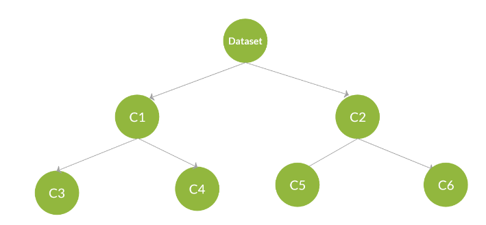
Figure 1: This figure demonstrates the recursive nature and a sample tree structure of the MSMBTAI.

In order to evaluate the efficacy of a clustering based anomaly detector, the Cluster-Based Local Outlier Factor (CBLOF)metric proposed by (He et al., 2003) has been used extensively. We propose the Enhanced Cluster Based Local Outlier Factor (ECBLOF), a modified CBLOF metric, where we avoid the multiplication with the cluster size since such a score can bias towards the large clusters. The following example explains the rationale.

Example 1

Suppose that a small cluster $C_{1}$ has only one data point $a$ which is an anomaly. Consider another large cluster $C_{2}$ with a non-anomalous data point $b\in C_{2}$. Suppose that the distance between $a$ and centroid of $C_{2}$ cluster is 10 ($d(a,C_{2})=10$). Since $C_{2}$ is the nearest larger cluster, as per the definition of the CBLOF, the anomaly score of $a=10\times 1$, whereas that of $b=1*|C_{2}|$ (since $b\in C_{2}$, its distance from the centroid of $C_{2}$ will be 1). If $|C_{2}|>10$, then $a$ will not be identified as an anomaly based on the CBLOF score and a normal data point $b$ will be considered as anomaly because of the higher anomaly score.

The modified metric called ECBLOF is defined below: Let $D$ be the dataset, partitioned into $n$ clusters $C_{1},\cdots,C_{i}\cdots,C_{n}$. We categorize the set of clusters into two, namely Small Cluster (SC)and Large Cluster (LC). For a predefined threshold $\alpha$, $C_{i}\in SC$ if $|C_{i}|<\alpha|D|$, otherwise it is in $LC$. For a data point $p\in D$, we define $ECBLOF(p)$ as

$$\begin{aligned} ECBLOF(p)=\begin{cases}\quad min(d(p,C_{j}))\ if\ C_{i}\in SC\\ \quad where\quad p\in C_{i}\wedge C_{j}\in LC\\ \quad\forall j=1\cdots b\end{cases}\end{aligned}$$ (1)

$$\begin{aligned} ECBLOF(p)=d(p,C_{i})\ if\ C_{i}\in LC\ where\ p\in C_{i}\end{aligned}$$ (2)

$d(p,C_{j})$ computes the distance between p and the cluster center of $C_{j}$.

Anomaly Detection using MSMBTAI:

The entire anomaly detection process is divided into two phases. First phase is the construction of the Anomaly Tree (AT)using the proposed MSMVMCA. In the second phase, MSMBTAI tries to find the probable anomalies using the ECBLOF metric. Algorithm 2 constructs the AT and a similar tree structure of the AT is demonstrated in Fig. 1. The algorithm terminates further clustering when the node level is more than $n$.

1 $v\leftarrow$ new Node()

2 $v.level\leftarrow L$

3 $v.cluster\leftarrow D$

4 if ($L\leq n$) then

       $(D_{L},D_{R})\leftarrow$MSMVMCA(D,2) $\triangleright$ $D_{L},D_{R}$ are two clusters generated by clustering function

5       $v.left\leftarrow AT(D_{L},n,L+1$)

6       $v.right\leftarrow AT(D_{R},n,L+1$)

7      

return $v$

Algorithm 2 AT($D,n,L$)

Algorithm 3 finds the leaf nodes from the AT and applies ECBLOF on all the leaf nodes. It applies anomaly ranking on the data points by sorting the dataset in descending order based on ECBLOF score.

Result: Probable anomaly data-points

1 $L\leftarrow 0$

2 $AT\_root\leftarrow$AT(D, L, n)

3 $leaf\_nodes\leftarrow$find_leaves($AT\_root$)

4 anomaly_score $\leftarrow$ ECBLOF(leaf-nodes)

5 anomaly_score $\leftarrow$ descending-sort(anomaly-score)

$\triangleright$ This function sorts the data-instances based on anomaly scores in descending order. Data-instances with higher anomaly scores take the top positions.

6

return Top_N(anomaly-score)

Algorithm 3 MSMBTAI($D,n$)

4 Data and Experiments

Table 2: A sample of anomalous exoplanets and statistics for the complete anomalous set for Dataset D1 including Surface Temperature and Surface Flux. In total, 51 anomalies are detected out of 1682 exoplanets.

Planet	Class	LOF	K-NN- ECBLOF	HBOS	iForest	MSMBTAI
KIC-5522786 b	thermoplanet	16	13	12	11	14
LHS 1140 b	psychroplanet	535	93	38	57	21
Proxima Cen b	psychroplanet	273	56	141	111	23
TRAPPIST-1 d	mesoplanet	201	45	9	63	42
TRAPPIST-1 e	psychroplanet	218	44	20	65	44
TRAPPIST-1 f	psychroplanet	215	40	19	64	50
tau Cet e	mesoplanet	442	248	80	43	67
K2-18 b	mesoplanet	366	283	336	286	171
Kepler-61 b	mesoplanet	445	384	260	486	538
Min		16	3	9	11	14
Max		1485	816	1334	763	664
Mean		440.14	263.39	335.80	273.94	215.51
StdDev		396.84	176.73	329.34	180.20	175.60
Range		16–1485	13–816	9–1334	11–763	14–664

Table 3: A sample of anomalous exoplanets and statistics for the complete anomalous set for Dataset D1 excluding Surface Temperature and Surface Flux. In total, 51 anomalies are detected out of 1682 exoplanets.

Planet	Class	LOF	K-NN- ECBLOF	HBOS	iForest	MSMBTAI
KIC-5522786 b	thermoplanet	12	13	37	13	12
Proxima Cen b	psychroplanet	288	43	85	83	17
LHS 1140 b	psychroplanet	415	84	125	50	21
TRAPPIST-1 d	mesoplanet	200	45	9	42	37
TRAPPIST-1 e	psychroplanet	203	48	18	49	73
TRAPPIST-1 f	psychroplanet	205	44	64	61	44
tau Cet e	mesoplanet	477	203	107	47	68
K2-18 b	mesoplanet	487	247	176	294	206
Kepler-61 b	mesoplanet	444	373	210	461	563
Min		12	13	9	13	12
Max		1605	838	646	641	644
Mean		412.82	257.24	262.33	247.33	205.90
StdDev		347.29	188.11	147.05	138.68	161.93
Range		12–1605	13–838	9-646	13–41	12–644

Dataset:

PHL-EC catalog serves as one of the most comprehensive datasets comprising both measured and derived features for exoplanets and their host stars. The catalog provides 68 features for the confirmed exoplanets: 13 categorical features and 55 continuous features, however, not every entry has all the features. Sometimes there are missing values for Eccentricity or Surface Temperature, for example. In the catalog, all planets are sorted into five categories based on their thermal surface characteristics: non-habitable, and potentially habitable: psychroplanet, mesoplanet, thermoplanet and hypopsychroplanet. For reasons stated in Section 2.2, we analyse the contribution of the surface temperature as a feature in an unsupervised setting in the experiments presented below, and only consider planets whose surface temperatures are measured, and not estimated.

This paper presents results based on two versions of this dataset (D1 and D2), both of which are described below. It is important to note that in both of the experiments with D1 and D2, features serving as measured markers for habitability, such as Star’s Habitable Zone (HZ) and Earth Similarity Index (ESI) were removed. (See Appendix B for the features from D1 and D2 used in the experiments.)
Dataset D1: The 2018 iteration of the PHL-EC dataset, containing Surface Temperature and Stellar Flux parameters, classifies 1681 planets into 5 habitable classes based on their surface temperatures, out of which 1631 are non-habitable. The disadvantage of class imbalance in the dataset (non-habitable: 1631, mesoplanets: 30, psychroplanets: 16, thermoplanets: 3, hypopsychroplanets: 2) hinders the robustness of any classifier in the absence of surface temperature. To compare the effect of Surface Temperature and Stellar Flux, the results include two sets of inferences from this data set, one including the above mentioned features and one without it, after the class labels are removed.

Dataset D2: The latest version contains 4048 exoplanets and classifies planets into three classes, non-habitable planets constituting a majority (3993). The current version does not include Surface Temperature and even such important characteristics as Gravity, Density, or Escape Velocity, are available for only 706 out of 4048 of these exoplanets. Hence, only one set of inferences covering these 706 exoplanets is drawn, out of which only 6 intersect with the optimistic/conservative list of exoplanets in the PHL-HEC. Only 93 of the 706 exoplanets intersect with D1 dataset.

Table 4: A sample of anomalous exoplanets and statistics for the complete anomalous set for Dataset D2 containing 6 anomalies in 706 exoplanets.

Planet	LOF	K-NN- ECBLOF	HBOS	iForest	MSMBTAI
K2-18 b	174	134	213	132	46
TRAPPIST-1 f	70	67	105	69	54
TRAPPIST-1 g	73	71	107	72	67
LHS 1140 b	156	52	160	55	68
TRAPPIST-1 d	67	65	108	65	81
TRAPPIST-1 e	68	66	104	73	85
Min	67	52	104	55	46
Max	174	134	213	132	85
Mean	101.33	75.83	132.83	77.67	66.83
StdDev	49.69	29.21	44.84	27.41	15.04
Range	67–174	52–134	104–213	55–132	46–85

Preprocessing:

In the Dataset D1, meso, thermo, psychro, and hypopsychro exoplanets are marked $1$ (anomalies) and all the non-habitable planets are marked $0$. Out of all the 1682 planets, any feature having data for less than 1600 planets is removed. Features not affecting habitability in any way as well as highly correlated features are also removed. 10 features are retained after Principal Component Analysis for both datasets to ensure fairness. For the Dataset D2, both conservative and optimistic habitable planets are considered as anomalies (marked 1) and all others are considered as normal instances (marked 0). These markers are not used only for cross-matching purposes. Only 706 of the exoplanets having non-null/non-missing values for important characteristics, such as Density and Gravity, are considered. Features irrelevant for habitability (Date of Discovery, etc.) as well as categorical features are removed. Finally, highly correlated features are removed.

5 RESULTS:

The proposed solution MSMBTAI is compared with Local Outlier Factor (LOF)(Ramaswamy et al., 2000), ECBLOF, HBOS (Goldstein and Dengel, 2012), and iForest (Liu et al., 2008). LOF, and ECBLOF are clustering based anomaly detection algorithms and these algorithms rely on a solution to identify anomalies. The solution applied is K-NN as an auxiliary tool in these approaches to identify anomalies. The results will be discussed in two parts, by comparing MSMBTAI and other clustering algorithms, and secondly discussing the effect of exclusion of surface temperature and stellar flux parameters. Since the range of anomaly scores can vary between algorithms, the results are discussed in terms of anomaly rank: a ranking based on the anomaly score obtained from an algorithm, with the lower anomaly rank indicating higher chance of a sample being anomalous, i.e. habitable. Consider the following definitions used in summarizing the results in the table:

• Min: Minimum anomaly rank among all anomalous planets

• Max: Maximum anomaly rank among all anomalous planets

• Mean: Average anomaly rank among all anomalous planets

• StdDev: Standard deviation of anomaly ranks among all anomalous planets

• Range: Maximum-Minimum anomaly rank of all anomalous planets

In Table 2, MSMBTAI produces better result in comparison to other algorithms in multiple parameters. iForest achieves the lowest maximum rank and MSMBTAI achieves the minimum mean rank in Table 3. MSMBTAI, among all algorithms, also assigns the lowest rank to such promising potential habitable exoplanets as Proxima Cen b and the TRAPPIST-1 planets.

Surface Temperature and Stellar Flux serve as hard markers for classification of exoplanets as habitable. Hence, after removing these features, the algorithms are expected to perform significantly worse. However, comparing Table 2 and Table 3, most algorithms perform very similar or even better after excluding parameters of surface temperature and stellar flux. We note that MSMBTAI assigns lowest rank to Proxima Cen b, tau Cet e and TRAPPIST-1 exoplanets. The nominal differences between the two tables indicate that sufficient clustering information can be obtained from the observed features alone, and fine-tuned unsupervised methods can be used in the future to indicate habitability of newly observed exoplanets. The results are especially motivating for the scientific community as features indicating habitability, such as minimum and maximum habitable zone of a star and similarity indices, like ESI, are not included in either of the computations.

Table 5: Description of the parameters of employed algorithms and their values for exoplanet datasets.

Algorithm	Parameter Description	Values in D1, D2
MSMBTAI($n$)	$n$: the maximum tree level	(4)
MSMVMCA	$v$: the number of versions in the population,
($v,s_{1},s_{2},n_{1},n_{2},F_{t}$)	$s_{1}$, $s_{2}$: proportions of stage1 and stage2	($12,0.5,0.5,10,10,0.5$)
	populations becoming parent,
	$n_{1}$, $n_{2}$: max iterations number of stage1 and stage2,
	$F_{t}$: the fitness threshold.
LOF$(k)$	$k$: number of neighbours included in density computation	(Average over 10–25)
HBOS$(bins,tolerance)$	$bins$: number of histogram bins to form,
	$tolerance$: determines the flexibility while	(10,0.5)
	dealing with samples lying outside the bins.
iForest$(estimators,samples)$	$estimators$: number of trees in the ensemble,
	$samples$: number of samples drawn to train	(100,256)
	each base estimator.

6 Conclusion

Earth-like rocky planets could amount to as many as 6 billion in the Milky Way (Kunimoto and Matthews, 2020; Bryson et al., 2020). Numerous space missions, current and planned for near future, are searching for potentially-habitable planets, for the possibility of exolife – life elsewhere in the Universe. Humanity is also looking for the second ‘Earth’ – a planet habitable for us, but preferably uninhabited, so that colonization opportunities, initially postulated by Krugman (2010) and recently considered through a quantitative model (Khaidema et al., 2021), can be explored. Inferences in astronomy do not rely absolutely on machine learning methods but benefit a great deal from such methods. It is the combination of ML-based inferences and domain knowledge that help reduce the search for habitable planets significantly due to the proposed method. Therefore, the outcome of MSMVMCA-based Anomaly detection is promising and relevant for the scientific community. The results from the clustering based algorithm were cross-matched with both optimistic and conservative lists of PHL-HEC habitable exoplanets. There are 42 matches out of 51 in the D1 set, and all 6 anomalies detected in D2 set match with PHL-HEC potentially habitable planets. Out of 6 discovered anomalies in D2, TRAPPIST-1 g planet is the only mismatch with D1. This means that Trappist 1-g is not detected as an anomaly in D1 dataset, but is detected as an anomaly when MSMA is applied on D2 dataset. This is an interesting observation, as Trappist 1-g is may be too cold to host life – its equilibrium temperature is 198.6 K (-75°C) (e.g. Wolf (2017)). In fact, it is deemed not habitable by the Solar Equivalent Astronomical Unit (SEAU) criteria (Yamashiki et al., 2017). The anomalous instances are cross-validated with domain knowledge-based expectations of habitable candidates and not by commonly used metrics, as the class labels in the PHL-EC are not beyond reasonable doubt. We have also shown the efficacy of our clustering method on additional datasets. As future work, the following will have to be considered:

1. It is required to improve the computation cost of the MSMVMCA in comparison to other clustering algorithms.

2. MSMVMCA has established itself as a clustering algorithm and been applied in detection of anomalous exoplanets. However, clustering algorithms such as K-means, K-medoids have been employed extensively in various domains, and it is required to implement MSMVMCA in other research domains as well to emphasize its strength.

Data Availability

Data and the codes associated with this manuscript are available on several websites:
1. CDHS/CEESSA Datasets and Catalogs: AstrIRG (Astroinformatics Research Group) website, http://astrirg.org/projects.html
2. Codes to analyze exoplanetary data from PHL’s HEC catalog: https://github.com/SuryodayBasak/Exoplanets
Analysis/tree/master/MLAnalysis

Appendix A MSMVMC Qualify as a Clustering Algorithm

Before applying on the exoplanet data, it was crucial to verify the effectiveness of the MSMVMCA as a clustering algorithm by applying it on various benchmark datasets. MSMVMCA has been applied on Iris, Glass, Seed, Knowledge, Libras, and Sonar datasets (Dua and Graff, 2019). These are benchmark data sets used extensively in machine classification (see the detailed description of each dataset in subsection  A.1). MSMVMCA has been also compared with other standard clustering algorithms such as K-means, K-medoids in terms of Rand and Jaccard indices – two metrics widely used in the performance comparison.

• Rand Index: A Rand index is used to measure the similarity between two data clusterings. The Rand index is related to the clustering accuracy though it can be applied when class labels are not available. The range of the Rand index is 0 to 1. Higher the value, better the accuracy of the data clustering.

• Jaccard Index: A Jaccard index is a statistical tool used to measure the similarity and diversity of sets. It is also known as a Jaccard coefficient. It is used to compare the similarity between finite sets. It is defined as the size of the intersection divided by the size of the union of the comparing sets. The range is from 0% to 100%. The higher the percentage, the more similarity between the two datasets.

Two different types of fitness functions are employed in stages. The first stage has used Silhouette, and the second stage has implemented Davis-Bouldin (DB) as a fitness function (See Appendix D for more details on the fitness functions). A higher Silhouette value means it has achieved better clustering, whereas a smaller DB value indicates a better result. We have assumed that the data points which belong to the same clusters are co-located together. For example, a dataset of 10 data points, where the first 2 data points belong to clusters1, the next 5 data points belong to cluster 3, and the last 3 data points are part of cluster 2. The order looks as follows: 1133333222. The result has been demonstrated in Table 6, and it is evident from the table that MSMVMCA has outperformed other clustering algorithms.

Table 6: MSMVMCA performance on benchmark data: MSMVMCA outperformed other algorithms in terms of both Jaccard and Rand coefficients.

Dataset	MSMVMCA		K-means		K-medoids
	Rand	Jaccard	Rand	Jaccard	Rand	Jaccard
Iris	0.9186	0.9333	0.8797	0.44	0.8922	0.4266
Glass	0.7665	0.2663	0.6718	0.2429	0.7302	0.1869
Seed	0.9566	0.3380	0.8743	0.0142	0.8713	0.2714
Knowledge	0.8099	0.6551	0.7590	0.2068	0.7181	0.5241
Libras	0.9125	0.1166	0.8911	0.1083	0.8748	0.1
Sonar	0.5094	0.5769	0.5032	0.4471	0.5054	0.5625

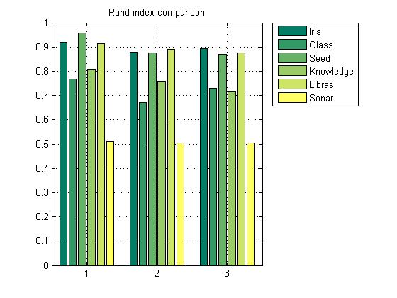
Figure 2: Comparison of MSMVMCA performance with K-means and K-medoids. The $X$-axis is the algorithm, where 1, 2 and 3 represent MSMVMCA, K-means and K-medoids, respectively. The $Y$-axis represents the Rand index. It is evident that MSMVMCA has achieved a higher Rand index in comparison to other algorithms.

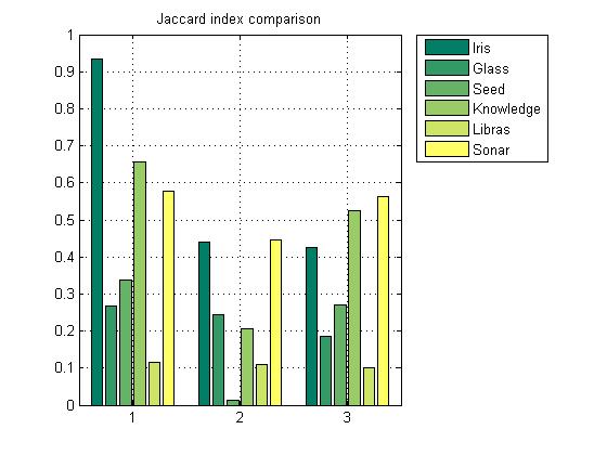
Figure 3: Comparison of MSMVMCA Jaccard index with K-means and K-medoids. Here, 1, 2 and 3 in $X$-axis denote MSMVMCA, K-means and K-medoids, respectively. $Y$-axis is the Jaccard index. MSMVMCA has attained a better result in comparison to other standard algorithms.

A.1 Description of Datasets

A.1.1 Iris

Iris is a well-known dataset used widely for clustering purposes in the field of pattern recognition. It has a total of 150 data points and 4 attributes. The total of three classes, each containing 50 data instances, were used for the task of anomaly detection. It is evident from Table 6 that MSMVMCA has achieved higher accuracy in both the Rand as well as Jaccard indices. For example, MSMVMCA has achieved Rand index 0.91, whereas K-means achieves 0.87 and K-medoid achieves 0.89. MSMVMCA has considered 100 versions in the initial population, where every chromosome, or version, was generated randomly. As we have assumed that the data points belonging to the same clusters are co-located, the initial population is generated in the same fashion. For example, version 1 randomly decided that the first 10 data instances are cluster 1, the next 100 belong to cluster 2, and the rest of the data instances are part of cluster 3. The same methodology has been applied to all other datasets to maintain uniformity. For both stages, Davis-Bouldin was used as a fitness function. However, the best version is selected from the population based on the Silhouette score.

A.1.2 Seed

This dataset comprises kernels belonging to three different types of wheat, with total of 210 data instances and 7 attributes. The dataset has three clusters, each having 70 data points. The MSMVMCA considered 100 version and Silhouette and DB as fitness functions in stage 1 and stage 2, respectively. MSMVMCA has attained 0.95 Rand index, which is higher than 0.87 achieved by both K-means and K-medoids.

A.1.3 Sonar

This sonar dataset consists of 208 records and 60 attributes. All these data instances belong to two classes, either Rock or Metal. Out of all these records, 111 data points were obtained by bouncing sonar signals off a metal cylinder at various angles and under various conditions. 97 records have been obtained from rocks under similar conditions. It is apparent from Table 6 that our proposed algorithm has outperformed K-means, K-medoids in terms of both Rand and Jaccard indices.

A.1.4 Libras

Libras comprises 360 data instances, and the total number of attributes is 91, which is higher than previous datasets. It contains 15 classes, each with 24 data points, and each class is a reference to a hand movement type in Libras. MSMVMCA attains higher accuracy in both Rand and Jaccard indices.

A.1.5 Knowledge

This dataset has 403 records, and the total number of attributes is 5. It has a total of 4 classes (Very Low, Low, Middle, High). Very Low has 50 instances, Low has 129 instances, Middle and High have 122 and 130 instances, respectively. MSMVMCA reached 0.80 in the Rand index, which is almost 0.09 more than K-medoids, and in the case of Jaccard index, the MSMVMCA has three times higher value than K-means.

A.1.6 Glass

The Glass dataset contains a total of 214 instances, and the total number of attributes is 10. This dataset is used extensively by many researchers in their papers. The same algorithms have been applied to the Glass dataset to evaluate the performance of the K-means algorithm after the dimension reduction. The types of glass present in the aforementioned dataset are

1. building_windows_float_processed

2. building_windows_non_float_processed

3. vehicle_windows_float_processed

4. containers

5. tableware

6. headlamps

MSMVMCA has performed better than other well-known algorithms as is evident from Table 6. In Figures 2 and 3, MSMVMCA, K-means, and K-medoids are denoted as 1, 2, and 3, respectively.

A.2 Setting Parameters for Different Datasets

The parameter settings for K-medoids and K-means algorithms for different datasets are shown in Table 7. MSMVMCA algorithm had the same parameter setup for all datasets: MSMVMCA($v,s_{1},s_{2},n_{1},n_{2},F_{t}$)=(100,0.5,0.5,10,10,0.7).

Table 7: Parameter settings on different datasets

Algorithm	Iris	Seed	Sonar	Knowledge	Glass	Libras
K-medoids ($k$)	(3)	(3)	(2)	(4)	(6)	(15)
K-means ($k$)	(3)	(3)	(2)	(4)	(6)	(15)

Appendix B List of features used in clustering Data sets D1 and D2 for anomalous (habitable) candidate detection

Features used for clustering for Dataset D1 (Features indicating (*) are included in one experiment and excluded in the other): Planet Mass, *Planet Stellar Flux (Mean), Star Size from Planet, Planet Radius, *Planet Surface Temperature (Mean), Star Temperature Effective, Planet Density, Planet Surface Pressure, Star Luminosity, Planet Gravity, Planet Period, Star Right Ascension, Planet Escape Velocity, Star Mass, Star Declination, Planet Semi Major Axis, Star Radius & Star Magnitude from Planet. Features used in MSMVMCA and other clustering techniques for Dataset D2:
Planet Mass, Star Radius, Planet Density, Planet Period, Star Temperature, Planet Distance, Star Right Ascension, Planet Escape Velocity, Planet Radius, Star Declination, Planet Potential (planet gravitational potential in earth units), Star Mass & Planet Gravity.

Appendix C Benchmark Methodologies: Anomaly Detection

This section describes various anomaly detection algorithms, which were used for comparison with MSMBTAI.

C.1 K-NN Global anomaly detection

For every data point, the $k$ nearest neighbors are calculated. The distance metric, e.g. L1, L2, Euclidean or Mahalanobis, can be decided according to the dataset. The anomaly score can be calculated according to measures described below:

1. largest: use the distance to the $k$-th neighbor as the outlier score

2. mean: use the average of all $k$ neighbors as the outlier score

3. median: use the median of the distance to $k$ neighbors as the outlier score

The anomaly score, however, is heavily dependent on normalization criteria and the number of dimensions. Another challenge is to be able to decide on the value of ‘$k$’. While in supervised algorithms, $k$ can be determined with cross-validation, deciding on a $k$ in unsupervised cases is more challenging. Hence, generally, an average over many values of $k$ is used to make a fair comparison with the rest of the algorithms. The algorithm performs well for global anomalies since for a data point to have a high score, it should be away from all the clusters in the dataset.

C.2 Local Outlier Factor (LOF)

As the name suggests, LOF is a local outlier scoring method that can be used for global anomalies as well. It is a density-based algorithm that relies on the $k$ nearest neighbors. The estimated local density of a point is the number of its neighbors divided by the cumulative sum of distances to its neighbors. LOF is then calculated by dividing the average density of the neighbors by the point’s density. Suppose $N(p)$ is the set of neighbors of point $p$, $k$ is the number of points in this set, and $d(p,x)$ is the distance between points $p$ and $x$. The estimated density is:

$$\hat{f}(p)=\frac{k}{\Sigma_{x\in N(p)}d(p,x)}\,,$$ (3)

and the local outlier factor score is:

$$LOF(p)=\frac{\frac{1}{k}\Sigma_{x\in N(p)}\hat{f}(x)}{\hat{f}(p)}\,.$$ (4)

Since LOF is a ratio of densities, normal instances would get a value close to 1, whereas outliers will get larger values. Here again, the value of $k$ needs to be adjusted.

C.3 Histogram-based Outlier Score (HBOS)

HBOS is a statistical algorithm, which calculates the anomaly score by creating a univariate histogram for each feature of the dataset, assuming independence of the features. The disadvantage of assuming feature independence becomes less severe when the dataset has a high number of dimensions, which is true for the case of the PHL-EC dataset. The density estimate is represented by the height of each bin of the histogram. For each feature, the histogram is normalized to $[0,1]$ and HBOS for each instance $v$ is computed as a product of the inverse of the estimated density:

$$HBOS(v)=\sum\limits_{i=0}^{d}\log{\left(\frac{1}{hist_{i}(v)}\right)}\,,$$ (5)

where $d$ is the number of dimensions, $v$ is the vector of features, and $hist_{i}(v)$ is the density estimate of each feature. Inverting the score ensures anomalies have a higher score than normal instances.

C.4 Isolation Forest

Isolation Forest is an ensemble method which ’isolates’ data points by randomly selecting a feature and then randomly selecting a split value to divide the data points into 2 nodes. Recursive partitioning will result in each observation residing in a leaf node, and the number of splittings required to isolate a sample is equal to path length from root to the leaf of the tree. If this length is averaged over a forest of many such random trees, it will act as a measure of the outlying behavior, producing shorter length for anomalies on average.

Appendix D Fitness Functions

D.1 Silhouette Index

The Silhouette index refers to the interpretation and validation of the consistency within the clusters of data. It measures how similar an object to its cluster (cohesion) in comparison to another cluster (separation). The ranges of the Silhouette vary from $-1$ to $+1$. A higher Silhouette indicates the object is matched perfectly to its cluster and poorly to other clusters. The value $+1$ means the sample is far away from the neighboring cluster and very close the cluster where it is assigned. $-1$ means the sample is near to the neighboring clusters and it is not so close to the assigned cluster. $0$ indicates that it is at the boundary of the distance two clusters. $+1$ is the ideal value and $-1$ is the least preferable. The higher the value, the better the clustering of the dataset. Assume the data has been partitioned into $K$ clusters using some standard clustering mechanism. Now, $i$ is a data-point and $a(i)$ is the average distance of all the data-points belong to the same cluster. $b(i)$ is the mean distance of the data point $i$ to all other data points of a neighboring cluster $(B)$ to which $i$ is not a member. And the neighbor cluster to which the data-point $i$ is closest in comparison to other clusters. The Silhouette can be calculated as follows,

$$s(i)=\frac{b(i)-a(i)}{max(b(i),a(i))}\,.$$ (6)

$s(i)$ will become $1$ if the $b(i)$ value is very large and $a(i)$ is very small: $b(i)>>a(i)$. This situation may happen when $a(i)$ is very close to other data points inside the cluster, and far away from the closest neighbouring cluster. This metric is used as a fitness function in stage1 in MSMVMCA.

D.2 Davis-Bouldin

Davis-Bouldin is a metric widely used for evaluating the clustering algorithm. It is the ratio between the within-cluster distances and the between-cluster distances. In the same way, it computes the average of the overall clusters and it is very easy to implement. The lower the score better the clustering (Davies and Bouldin, 1979). The lowest value of the Davis-Bouldin that can be achieved is $0$. We have considered this metric as a fitness function in stage 2 in the proposed algorithm.

References

- Basak et al. (2020) Basak, S., Saha, S., Mathur, A., Bora, K., Makhija, S., Safonova, M., Agrawal, S., 2020, Astronomy and Computing, 30, 100335
- Bora et al. (2016) Bora, K., Saha, S., Agrawal, S., Safonova, M., Routh, S., Narasimhamurthy, A., 2016, Astronomy and Computing, 17, 129
- Bryson et al. (2020) Bryson, S., Kunimoto, M., Kopparapu, R. K., Coughlin, J. L., Borucki, W. J., et al., 2020, AJ, 161(1), 36. DOI:10.3847/1538-3881/abc418
- Castellani et al. (2020) Castellani, A., Schmitt, S., Squartini, S., 2020, IEEE Transactions on Industrial Informatics, 1
- Davies and Bouldin (1979) Davies, D. L., Bouldin, D. W., 1979, IEEE Transactions on Pattern Analysis and Machine Intelligence, 1(2), 224. doi10.1109/TPAMI.1979.4766909
- Dua and Graff (2019) Dua, D., Graff, C., 2019, UCI Machine Learning Repository [http://archive.ics.uci.edu/ml]. Irvine, CA: University of California, School of Information and Computer Science
- Goldstein and Dengel (2012) Goldstein, M., Dengel, A., 2012. Histogram-based Outlier Score (HBOS): A fast Unsupervised Anomaly Detection Algorithm. In: Wölfl, S., ed, KI-2012: Poster and Demo Track. Online; pp. 59
- He et al. (2003) He, Z., Xu, X., Deng, S., 2003, Pattern Recognition Letters, 24(9–10), 1641
- Karczmarek et al. (2020) Karczmarek, P., Kiersztyn, A., Pedrycz, W., Al, E., 2020, Knowledge-Based Systems, 195, 105659. DOI: https://doi.org/10.1016/j.knosys.2020.105659
- Khaidema et al. (2021) Khaidem, L., Saha, S., Kar, S., Mathur, A., Saha, S., 2021, Eur. Phys. J. Spec. Top., https://doi.org/10.1140/epjs/s11734-021-00208-8
- Knorr and Ng (1998) Knorr, E. M., Ng, R. T., 1998, Proc. 24rd Int. Conf. Very Large Data Bases, August 24-27, 1998, San Francisco, CA., USA., pp. 392
- Krasnogor et al. (2006) Krasnogor, N., Aragn, A., Pacheco, J., 2006. Memetic Algorithms. In: Alba, E., Mart, R., eds, Metaheuristic Procedures for Training Neutral Networks. Operations Research/Computer Science Interfaces Series, vol. 36. Springer, Boston, MA
- Krugman (2010) Krugman, P., 2010, Economic Inquiry, 48, 1119. doi:10.1111/j.1465-7295.2009.00225.x
- Kunimoto and Matthews (2020) Kunimoto, M., Matthews, J. M., 2020, AJ, 159(6), 248. DOI: 10.3847/1538-3881/ab88b0
- Limbach et al. (2015) Limbach, A. M., Turner, L. E., 2015, PNAS, 112, 20
- Liu et al. (2008) Liu, T. F., Ting, M. K., Zhou, Z. H., 2008, Proc. 2008 Eighth IEEE International Conference on Data Mining (ICDM ’08). IEEE Computer Society, USA, 413. DOI:https://doi.org/10.1109/ICDM.2008.17
- Luhman et al. (2011) Luhman, K. L., Burgasser, A. J., Bochanski, J. J., 2011, ApJL, 730, L9. doi: 10.1088/2041-8205/730/1/L9
-
Méndez (2011)
Méndez, A., 2011, A Thermal Planetary Habitability Classification for Exoplanets, Planetary Habitability Laboratory @ UPR Arecibo. URL: http://phl.upr.edu/library/notes/athermalplanetary
habitabilityclassificationforexoplanets - Munir et al. (2018) Munir, M., Siddiqui, A. S., Dengel, A., Ahmed, S., 2018, IEEE Access, 1. doi:10.1109/access.2018.2886457
- Murthy and Chowdhury (1996) Murthy, C. A., Chowdhury, N., 1996, Pattern Recognition Letters, 17(8), 825
- Ramaswamy et al. (2000) Ramaswamy, S., Rastogi, R., Shim, K., 2000, ACM SIGMOD Record, 29, 427. DOI:https://doi.org/10.1145/335191.335437
- Saha et al. (2018) Saha, S., Basak, S., Safonova, M., Bora, K., Agrawal, S., Sarkar, P., Murthy, J., 2018, Astronomy and Computing, 23, 141
- Saha et al. (2020) Saha, S., Nagaraj, N., Mathur, A., Yedida, R., Sneha, H. R., 2020, Eur. Phys. J. Spec. Top., 229(16), 1. DOI: 10.1140/epjst/e2020-000098-9
- Spiegel and Turner (2012) Spiegel, D. S., Turner, E. L., 2012, PNAS, 109, 395. DOI: 10.1073/pnas.1111694108
- Tasker et al. (2017) Tasker, E., Tan, J., Heng, K., Kane, S., Spiegel, D., & the ELSI Origins Network Planetary Diversity Workshop, 2017, Nature Astronomy, 1, 0042. DOI:10.1038/s41550-017-0042
- Thinsungnoen et al. (2015) Thinsungnoen, T., Nuntawut, K., Pongsakorn, D., Kittisak, K., Nittaya, K., 2015, Proc. 2nd Int. Conf. Industrial Application Engineering 2015, pp. 44. doi:10.12792/iciae2015.012
- Wang et al. (2017) Wang, Y., Liu, Y., Tian, F., Hu, Y., Huang, Y., 2017, preprint (arXiv:1710.01405)
- Wolf (2017) Wolf, E. T., 2017, ApJL, 839, L1
- Yamashiki et al. (2017) Yamashiki, Y. Notsu, Y., Sasaki, T., et al., 2017, Radio Exploration of Planetary Habitability meeting (AASTCS5) held 7-12 May 2017, Miramonte Resort & Spa in Palm Spring, California, 49, 202.09
- Zhang et al. (2017) Zhang, L., Lin, J., Karim, R., 2017, IEEE Transactions on Systems, Man & Cybernetics Systems, ISSN 2168-2216, 47(2), 289, article id 7509594