Initial perturbation matters: implications of geometry-dependent universal Kardar-Parisi-Zhang statistics for spatiotemporal chaos

Abstract

Infinitesimal perturbations in various systems showing spatiotemporal chaos (STC) evolve following the power laws of the Kardar-Parisi-Zhang (KPZ) universality class. While universal properties beyond the power-law exponents, such as distributions and correlations, and their geometry dependence, are established for random growth and related KPZ systems, the validity of these findings to deterministic chaotic perturbations is unknown. Here we fill this gap between stochastic KPZ systems and deterministic STC perturbations by conducting extensive simulations of a prototypical STC system, namely the logistic coupled map lattice. We show that the perturbation interfaces, defined by the logarithm of the modulus of the perturbation vector components, exhibit the universal, geometry-dependent statistical laws of the KPZ class, despite the deterministic nature of STC. We demonstrate that KPZ statistics for three established geometries arise for different initial profiles of the perturbation, namely point (local), uniform, and “pseudo-stationary” initial perturbations, the last being the statistically stationary state of KPZ interfaces given independently of the Lyapunov vector. This geometry dependence lasts until the KPZ correlation length becomes comparable to the system size. Thereafter, perturbation vectors converge to the unique Lyapunov vector, showing characteristic meandering, coalescence, and annihilation of borders of piece-wise regions that remain different from the Lyapunov vector. Our work implies that the KPZ universality for stochastic systems generally characterizes deterministic STC perturbations, providing new insights for STC, such as the universal dependence on initial perturbation and beyond.

Many studies have been devoted to elucidating universal properties of spatially extended dynamical systems via statistical physics. In particular, seminal work by Pikovsky, Kurths, and Politi has demonstrated that infinitesimal perturbations to various dynamical systems showing spatiotemporal chaos (STC) evolve following universal power laws of the Kardar-Parisi-Zhang (KPZ) universality class, a representative universality class for stochastic processes Pikovsky and Kurths (1994); Pikovsky and Politi (1998). Though exact studies on stochastic interface growth have advanced the knowledge of the KPZ class dramatically Kriecherbauer and Krug (2010); Corwin (2012); Quastel and Spohn (2015); Halpin-Healy and Takeuchi (2015); Sasamoto (2016); Spohn (2017); Takeuchi (2018), revealing geometry-dependent but universal statistical properties beyond the power-law exponents, these developments have been attained independently from the field of dynamical systems. In this paper, we attempt to bridge those two subjects by extensive numerical simulations of the logistic coupled map lattice, a prototypical model of spatially extended dynamical systems Kaneko (1989, 1993). We first show clear evidence that the perturbations show the universal statistical properties of the KPZ class beyond the power-law exponents, and the geometry dependence manifests itself as the dependence on the initial profile of the perturbations. We then study the time regime in which the KPZ correlation length reaches the system size and found that the perturbations converge to a unique Lyapunov vector as suggested by Oseledec’s theorem Oseledec (1968); Eckmann and Ruelle (1985); Kuptsov and Parlitz (2012). We found that this process is governed by characteristic wandering and annihilation of the boundaries of the segmental regions that differ from the Lyapunov vector. With the current knowledge on KPZ and dynamical systems, we expect our results to generally hold in STC and can be extended to general initial perturbations.

I Introduction

To understand general laws governing spatially extended dynamical systems, it is insightful to focus on the thermodynamic limit. Successful approaches include applying the concept of phase transition to understand collective states Aranson and Kramer (2002); Chaté and Manneville (1987, 1988); Miller and Huse (1993); Marcq, Chaté, and Manneville (1996); *marcq_1997a and synchronization Pikovsky, Rosenblum, and Kurths (2003) in large dynamical systems. Considering the infinite-size limit is also crucial for defining the extensivity of chaos, by the existence of a finite density of Lyapunov exponents per degree of freedom Ruelle (1982); Manneville (1985); Egolf et al. (2000).

In particular, universality associated with scale invariance has successfully provided a general insight for growing infinitesimal perturbations in spatially extended dynamical systems. When a system is showing spatiotemporal chaos (STC), i.e., chaos characterized by spatial and temporal disorder, perturbations given to trajectories typically grow exponentially and fluctuate. Pioneering studies by Pikovsky, Kurths, and Politi Pikovsky and Kurths (1994); Pikovsky and Politi (1998) revealed that, for a wide range of systems, this growing perturbation belongs to the Kardar-Parisi-Zhang (KPZ) universality class Kardar, Parisi, and Zhang (1986), which is one of the most wide-ranging universality classes for various stochastic processes (see reviews Kriecherbauer and Krug (2010); Corwin (2012); Quastel and Spohn (2015); Halpin-Healy and Takeuchi (2015); Sasamoto (2016); Spohn (2017); Takeuchi (2018)), including growing interfaces, directed polymers, stochastic particle transport, nonlinear fluctuating hydrodynamics Spohn (2016, 2017), and most recently, to quantum spin chains Ljubotina, Žnidarič, and Prosen (2019); Scheie et al. (2021); Wei et al. (2021); Bulchandani, Gopalakrishnan, and Ilievski (2021), to name but a few.

To be more specific, let us focus on a system showing STC in one-dimensional space. The dynamical variable is $u(x,t)$ with position $x$ and time $t$. We consider an infinitesimal perturbation $\delta{}u(x,t)$, growing from a given initial perturbation $\delta{}u(x,0)$ applied to the trajectory. Then, Pikovsky and coworkers Pikovsky and Kurths (1994); Pikovsky and Politi (1998) studied fluctuations of $h(x,t):=\log\left|\delta{}u(x,t)\right|$, which we call the perturbation interface, and found universal power laws for the fluctuation amplitude $\sim{}t^{\beta}$ and the correlation length $\sim{}t^{1/z}$, with characteristic exponents $\beta=1/3$ and $z=3/2$ of the one-dimensional KPZ class. This emergence of KPZ fluctuations in STC perturbations has been found in a variety of systems, ranging from coupled map lattices (CML) Pikovsky and Kurths (1994); Pikovsky and Politi (1998); Szendro et al. (2007); Pazó et al. (2008); Pazó, López, and Politi (2013), a coupled ordinary differential equation Pazó et al. (2008); Pazó, López, and Politi (2013), partial differential equations Pikovsky and Politi (1998) to time-delayed systems Pikovsky and Politi (1998); Pazó and López (2010); Pazó, López, and Politi (2013).

However, this connection to the KPZ class has far-reaching implications, beyond the exponents. The understanding on the one-dimensional KPZ class has been completely renewed during the last decades, thanks to remarkable developments by exact solutions Kriecherbauer and Krug (2010); Corwin (2012); Quastel and Spohn (2015); Halpin-Healy and Takeuchi (2015); Sasamoto (2016); Spohn (2017); Takeuchi (2018). An important outcome is the determination of the distribution and correlation functions of the interface fluctuations, which turned out to be universal yet dependent on the initial condition Kriecherbauer and Krug (2010); Corwin (2012); Quastel and Spohn (2015); Halpin-Healy and Takeuchi (2015); Takeuchi (2018). More specifically, we can write down the interface height $h(x,t)$ for infinite-size systems, asymptotically, in the following form:

$$h(x,t)\simeq v_{\infty}t+(\Gamma t)^{1/3}\chi(X,t),$$ (1)

where $\chi(X,t)$ is a stochastic variable discussed below, $X:=x/\xi(t)$ is the coordinate rescaled by the correlation length $\xi(t):=\frac{2}{A}(\Gamma{}t)^{2/3}$, and $v_{\infty},\Gamma,A$ are system-dependent parameters Prähofer and Spohn (2000); Takeuchi (2018). Then, it has been shown both theoretically Kriecherbauer and Krug (2010); Corwin (2012); Takeuchi (2018) and experimentally Takeuchi (2018); Takeuchi and Sano (2010); Takeuchi et al. (2011); Takeuchi and Sano (2012); Fukai and Takeuchi (2017); Iwatsuka, Fukai, and Takeuchi (2020); Fukai and Takeuchi (2020) that statistical properties of $\chi(X,t)$ are universal but depend on the choice of the initial condition $h(x,0)$. The following constitute three canonical cases, dubbed universality subclasses: (i) the flat subclass for the flat initial condition $h(x,0)=0$; (ii) the circular subclass for wedge or curved initial conditions, e.g., $h(x,0)=-\kappa|x|$ or $-cx^{2}$; (iii) the stationary subclass for statistically stationary initial conditions. Note that such initial conditions typically take the form of $h(x,0)=\sqrt{A}B(x)$, where $B(x)$ is the standard Brownian motion characterized by $\langle[B(x+\ell)-B(x)]^{2}\rangle{}={}\ell$ and $B(0)=0$. This is true exactly of the KPZ equation Kardar, Parisi, and Zhang (1986); Barabási and H. Eugene Stanley (1995); Takeuchi (2018) and also valid for other models in coarse-grained scales. Then, for each subclass, the one-point distribution of $\chi(0,t\to\infty)$ is known to be (i) the Gaussian orthogonal ensemble (GOE) Tracy-Widom distribution Tracy and Widom (1996), (ii) the Gaussian unitary ensemble (GUE) Tracy-Widom distribution Tracy and Widom (1994), and (iii) the Baik-Rains distribution Baik and Rains (2000) (see Prähofer and Spohn (2000); Kriecherbauer and Krug (2010); Corwin (2012); Halpin-Healy and Takeuchi (2015); Takeuchi (2018)), denoted by the random variable $\chi_{1},\chi_{2},\chi_{0}$, respectively. These subclasses have also been characterized by correlation functions Kriecherbauer and Krug (2010); Corwin (2012); Quastel and Spohn (2015); Halpin-Healy and Takeuchi (2015); Sasamoto (2016); Spohn (2017); Takeuchi (2018), which continue attracting considerable attention (e.g., recent developments on time covariance Takeuchi and Sano (2012); Ferrari and Spohn (2016); De Nardis, Le Doussal, and Takeuchi (2017); Johansson (2019); Johansson and Rahman (2021); Liu (2019) and on general initial conditions Corwin, Quastel, and Remenik (2015); Dauvergne, Ortmann, and Virág (2019)).

With this background, the following questions arise: Does this initial-condition dependence of KPZ fluctuations show up in perturbation dynamics of STC? If yes, how? Moreover, since we expect that the vector direction of $\delta{}u(x,t)$ eventually converges to the unique Lyapunov vector associated with the largest Lyapunov exponent, as Oselsedec’s theorem Oseledec (1968); Eckmann and Ruelle (1985); Kuptsov and Parlitz (2012) suggests unless the largest exponent is degenerate, how does the initial-condition dependence of $\delta{}u(x,t)$ reconcile with this fact? In this article, we address these questions numerically by an extensive simulation of the CML of the logistic map, a prototypical model showing STC Kaneko (1989, 1993).

II Method

We employed the CML of the logistic map, defined as follows. The dynamical variables $u(x,t)\in[0,1]$ are defined for integer $x$ and $t$, with the periodic boundary condition $u(x,t)=u(\mathrm{mod}(x,L),t)$. Time evolution is

$$u(x,t+1)= (1-\epsilon)f(u(x,t))$$

$$\quad+\frac{\epsilon}{2}[f(u(x-1,t))+f(u(x+1,t))],$$ (2)

which is denoted by $F_{x}(u(0,t),\dots,u(L-1,t))$, with $f(u)=au(1-u)$ and parameters $\epsilon$ and $a$. Here we chose $a=4$ and $\epsilon=0.05$, for which this CML shows fully disordered STC Kaneko (1989, 1993). The evolution of infinitesimal perturbations $\delta u(x,t)$ is then given by $\delta u(x,t+1)=\sum_{x^{\prime}=0}^{L-1}\left.\frac{\partial F_{x}(u_{0},\dots,u_{L-1})}{\partial u_{x^{\prime}}}\right|_{u_{i}=u(i,t)}\delta u(x^{\prime},t).$

To discard the transient before we applied a perturbation at $t=0$, each simulation started at $t=-T_{\mathrm{warmup}}$ from an initial condition $u(x,-T_{\mathrm{warmup}})$ generated randomly and independently. We chose $T_{\mathrm{warmup}}=1000$ and checked that the system is already in the attractor at $t=0$, by comparing the histograms of $u(x,t)$ at $t=0$ and $t=10^{5}$ (Fig. LABEL:S-fig:z_histogram sup ). We then applied a perturbation $\delta u(x,0)$ that takes different forms as we describe below, obtained $\delta{}u(x,t)$, and analyzed fluctuations of $h(x,t)=\log\left|\delta u(x,t)\right|$.

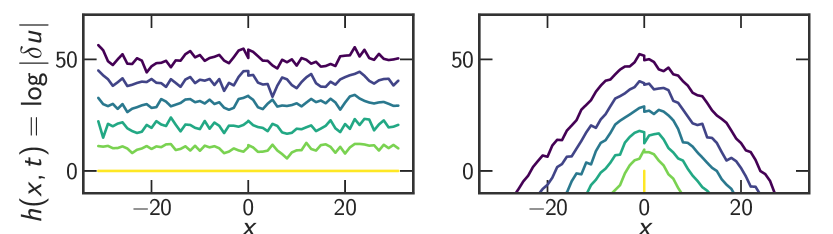
Figure 1: Typical snapshots of $h(x,t)=\log\left|\delta u(x,t)\right|$ from the uniform (left) and point (right) initial perturbations, at $t=0,20,\cdots,100$ from bottom to top.

III Uniform and point initial perturbations

We first studied the initial-shape dependence of STC perturbations. For this, we compare the uniform initial condition $\delta u(x,0)=1$ and the point initial condition $\delta u(x,0)=\delta_{x,0}$. Figure 1 shows typical snapshots of the perturbation interface $h(x,t)=\log\left|\delta{}u(x,t)\right|$ for those initial perturbations. We simulated $2400$ and $160000$ independent trajectories with $L=2^{15}$ and $L=2^{12}$ for the uniform and point perturbations, respectively.

First, we measured the mean height $\langle h(0,t)\rangle$, where $\langle\dots\rangle$ indicates the ensemble average. For the uniform perturbations, we also took the spatial average because of the translational symmetry. As expected, $\langle h(0,t)\rangle$ grows linearly with time, reflecting the exponential growth of the perturbation (Fig. LABEL:S-fig:raw_cumulants sup ). We also measured the variance $\langle h(0,t)^{2}\rangle_{\rm c}=\langle\delta h(0,t)^{2}\rangle$ with $\delta h(x,t){}:={}h(x,t)-\langle h(x,t)\rangle$ and the third- and fourth-order cumulants, $\langle h(0,t)^{3}\rangle_{\rm c}=\langle\delta h(0,t)^{3}\rangle$ and $\langle h(0,t)^{4}\rangle_{\rm c}=\langle\delta h(0,t)^{4}\rangle-3\langle\delta h(0,t)^{2}\rangle^{2}$. The $k$th-order cumulants ($k=2,3,4$) show power laws $\langle h(0,t)^{k}\rangle_{\rm c}\sim t^{k/3}$ characteristic of the KPZ class [Figs. 2(a) and LABEL:S-fig:raw_cumulants sup ], indicating that this exponent does not depend on the choice of initial perturbation, as expected.

We then investigated the one-point distribution of $h(0,t)$, measuring the skewness $\mathrm{Sk}[h(0,t)]\allowbreak:=\allowbreak\nicefrac{{\langle h(0,t)^{3}\rangle_{\rm c}}}{{\langle h(0,t)^{2}\rangle_{\rm c}^{3/2}}}$ and the kurtosis $\mathrm{Ku}[h(0,t)]\allowbreak:=\allowbreak\nicefrac{{\langle h(0,t)^{4}\rangle_{\rm c}}}{{\langle h(0,t)^{2}\rangle_{\rm c}^{2}}}$. Figure 2(b) shows that those for the uniform and point initial perturbation converge to the values for the flat ($\chi_{1}$) and circular ($\chi_{2}$) KPZ subclasses, respectively. This indicates that those perturbations indeed belong to the respective KPZ subclasses.

To characterize statistical properties further, we estimated the nonuniversal parameters, $v_{\infty}$, $\Gamma$, and $A$ Takeuchi (2018); Krug, Meakin, and Halpin-Healy (1992). These parameters are expected to be independent of the initial perturbation Krug, Meakin, and Halpin-Healy (1992); Takeuchi and Sano (2012); Takeuchi (2018). First we estimated the asymptotic growth speed $v_{\infty}$, which corresponds to the Lyapunov exponent in the limit $L\to\infty$. To do so, we used the local Lyapunov exponent $\lambda(t):=\langle\frac{\partial h(0,t)}{\partial{}t}\rangle$, which satisfies, for sufficiently large systems, the following relation derived from Eq. (1):

$$\lambda(t)=v_{\infty}+\mathrm{const.}\times t^{-2/3}.$$ (3)

Using this, we estimated $v_{\infty}$ by linear regression of $\lambda(t)$ against $t^{-2/3}$ [Fig. 2(c)]. We thereby obtained $v_{\infty}=0.53249(2)$ and $0.53250(7)$ for the uniform and point initial perturbations, respectively, where the numbers in the parentheses indicate the estimation uncertainty. This confirms that $v_{\infty}$ does not depend on the initial perturbation. Next, we estimated $\Gamma$ by $\nicefrac{{\langle h(0,t)^{2}\rangle_{\rm c}}}{{(\langle\chi_{j}^{2}\rangle_{\rm c}t^{2/3})}}\simeq\Gamma^{2/3}$ derived from Eq. (1), using $\chi_{1}$ and $\chi_{2}$ for the uniform and point initial perturbations, respectively. Similarly to other KPZ interfaces Takeuchi (2018); Takeuchi and Sano (2012); Ferrari and Frings (2011), the quantity in the left-hand side shows finite-time corrections in the order of $\mathcal{O}(t^{-2/3})$ (Fig. LABEL:S-fig:Gamma_estimation sup ). Therefore, by linear regression against $t^{-2/3}$, we obtained $\Gamma=0.1373(5)$ and $0.1369(6)$ for the uniform and point initial perturbations, respectively. From this, we derived the final estimate $\Gamma=0.1371(9)$. Finally, we estimated $A$ from the asymptotic growth speed for the finite-size systems, or the Lyapunov exponent, $\lambda_{\infty}(L):=\lim_{t\to_{\infty}}\langle\frac{\partial h}{\partial t}\rangle$. First, note that Eq. (3) for $\lambda(t)$ is expected to hold until the correlation length $\xi(t)$ reaches the system size $L$. Beyond this, $\lambda(t)$ will deviate from Eq. (3) and converge to $\lambda_{\infty}(L)\simeq v_{\infty}-\frac{A\tilde{\lambda}}{L}$, where $\tilde{\lambda}$ is a parameter satisfying $\Gamma=\frac{A^{2}\left|\tilde{\lambda}\right|}{2}$ Krug, Meakin, and Halpin-Healy (1992); Takeuchi (2018). Our simulations for the uniform initial perturbation (see Table LABEL:S-tab:lambda_estimation_params sup for parameter values) confirmed that $\lambda_{\infty}(L)$ depends linearly on $L^{-1}$ [Fig. 2(c) inset]. By linear regression, we obtained $A\tilde{\lambda}=0.0744(3)$ and $v_{\infty}=0.5324985(7)$, the latter refining our previous estimates. From the estimates of $A\tilde{\lambda}$ and $\Gamma$, we obtained $A$ by $A=\frac{2\Gamma}{A\tilde{\lambda}}$.

With those parameters, we defined the rescaled height

$$q(0,t):=\frac{h(0,t)-v_{\infty}t}{(\Gamma t)^{1/3}}\simeq\chi(0,t)$$ (4)

and investigated its statistical properties. Figure 2(d) shows its one-point distribution (again taking all $X$ for the uniform perturbation). The distributions for the uniform and point initial perturbation agree with those of the exact solutions for the flat and circular subclasses, namely the GOE and GUE Tracy-Widom distributions, respectively. Accordingly, the first- to fourth-order cumulants of $q(0,t)$ converge to those of $\chi_{1}$ and $\chi_{2}$, respectively (Fig. LABEL:S-fig:rescaled_cumulants sup ). We also measured spatial and temporal correlation functions and found agreement with the known results for the flat and circular subclasses (see Supplemental Text sup ). These results clearly indicate that the statistical properties of perturbation dynamics for the uniform and point initial perturbation are governed by the flat and circular KPZ subclasses, respectively.

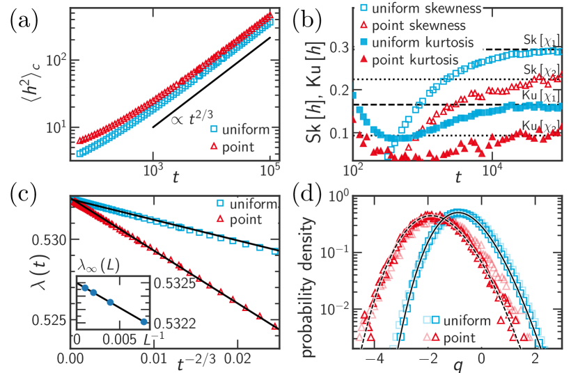
Figure 2: Results for the uniform and point initial perturbations. (a) The variance of the height $h(0,t)$. The black line is a guide to eyes indicating the power law $t^{2/3}$. (b) The skewness $\mathrm{Sk}[h(0,t)]$ and the kurtosis $\mathrm{Ku}[h(0,t)]$ of the height distribution. The values for $\chi_{1}$ and $\chi_{2}$ are shown by the dashed and dotted lines, respectively. (c) The local Lyapunov exponent $\lambda(t)$ plotted against $t^{-2/3}$. The black lines are the results of the linear fit. (inset) The infinite-time Lyapunov exponent $\lambda_{\infty}(L)$ plotted against $L^{-1}$. The black line is the result of the linear fit used for the estimation of $A\tilde{\lambda}$ and $v_{\infty}$. (d) The rescaled height distribution at $t=10^{3}$ (lighter color) and $t=10^{5}$ (darker color), for the uniform (turquoise squares) and point (red triangles) perturbations. The probability density function of $\chi_{1}$ and $\chi_{2}$ (GOE and GUE Tracy-Widom distributions, respectively) is shown by the solid and dashed lines, respectively.

IV Pseudo-stationary initial perturbation

From the viewpoint of dynamical systems theory, the perturbation interfaces are expected to converge to the unique Lyapunov vector (unique at each point in phase space), associated with the largest Lyapunov exponent Eckmann and Ruelle (1985); Kuptsov and Parlitz (2012). On the other hand, KPZ interfaces generally have a statistically stationary state, characterized by the time-invariance of the equal-time probability distribution of the height fluctuations. For the KPZ equation, such a stationary state is given by the Brownian motion Kardar, Parisi, and Zhang (1986); Barabási and H. Eugene Stanley (1995); Takeuchi (2018), $h(x,\cdot)=\sqrt{A}B(x)$, as already described. This is characterized by the scaling law for the height-difference correlation function

$$C_{h}(\Delta x,t):=\langle[h(x+\Delta x,t)-h(x,t)]^{2}\rangle\simeq A\Delta x,$$ (5)

which generally holds in the stationary state of the one-dimensional KPZ class Barabási and H. Eugene Stanley (1995); Kriecherbauer and Krug (2010); Corwin (2012); Quastel and Spohn (2015); Halpin-Healy and Takeuchi (2015); Sasamoto (2016); Spohn (2017); Takeuchi (2018). However, since the notion of Brownian motion can be defined only by the ensemble of realizations, for STC perturbations, it does not specify the unique realization corresponding to the Lyapunov vector. In other words, all realizations of the Brownian motion except the one corresponding to the true Lyapunov vector are not the stationary state of the perturbation interfaces. It is therefore natural to ask whether such pseudo-stationary states, generated randomly irrespective of the state of the dynamical system, may exhibit the characteristic fluctuation properties of the stationary KPZ subclass.

To answer this, we studied perturbation interfaces from pseudo-stationary initial conditions, given independently of the state of the dynamical system. Using the estimated value of $A$, we prepared a pseudo-stationary initial perturbation $h_{0}(x)=\sqrt{A}B(x)$ with $h_{0}(0)=0$ and the periodic boundary condition (see Supplemental Text sup ), and set the initial perturbation by $\delta u(x,0)=\exp[h_{0}(x)]$. Figure 3(a) illustrates the perturbation interface for such a pseudo-stationary initial condition. We simulated 2400 sets of independent trajectories and pseudo-stationary initial perturbations, with $L=2^{15}$. To evaluate systematic error due to the uncertainty of $A$ in $h_{0}(x)=\sqrt{A}B(x)$, we also ran simulations with the value of $A$ replaced with its upper and lower bounds of the range of uncertainty, 2400 realizations each.

We first checked the statistical stationarity of perturbation interfaces from such pseudo-stationary initial conditions. Figure 3(b) shows that $C_{h}(\Delta x,t)/\Delta x$ at $t=10^{4}$ and $10^{5}$ are identical in the pseudo-stationary case, keeping $C_{h}(\Delta{}x,t)/\Delta{}x\simeq{}A$ for $\Delta{}x\ll{}L$. Figure 3(c) shows that the growth speed, or the local Lyapunov exponent, takes a constant value only after a very short period. These results demonstrate the statistical stationarity of our pseudo-stationary interfaces.

We then compared the statistical properties of the perturbation interfaces with the predictions for the KPZ stationary subclass. In the following, the statistical accuracy was improved by taking advantage of translational symmetry, which guarantees that $h(x,t)-h_{0}(x)$ is equivalent to $h(0,t)$. We first measured the skewness and kurtosis of $h(0,t)$ and found convergence to those of $\chi_{0}$, i.e., the Baik-Rains distribution characterizing the stationary subclass [Fig. 3(d) inset]. We also confirmed agreement with the Baik-Rains distribution, by histograms [Fig. 3(e)] and cumulants (Fig. LABEL:S-fig:rescaled_cumulants sup ) of the rescaled height $q(0,t)$. Agreement with the stationary KPZ subclass was also confirmed through correlation functions (see Supplemental Text sup ), notably by quantitative agreement to the exact solution of the two-point space-time correlation Prähofer and Spohn (2004). These results demonstrate that the perturbation interfaces from the pseudo stationary initial conditions are indeed governed by the stationary KPZ subclass, despite not being stationary for the dynamical system. Of course, one can also start with the true Lyapunov vector as an initial perturbation and the same KPZ stationary subclass is expected.

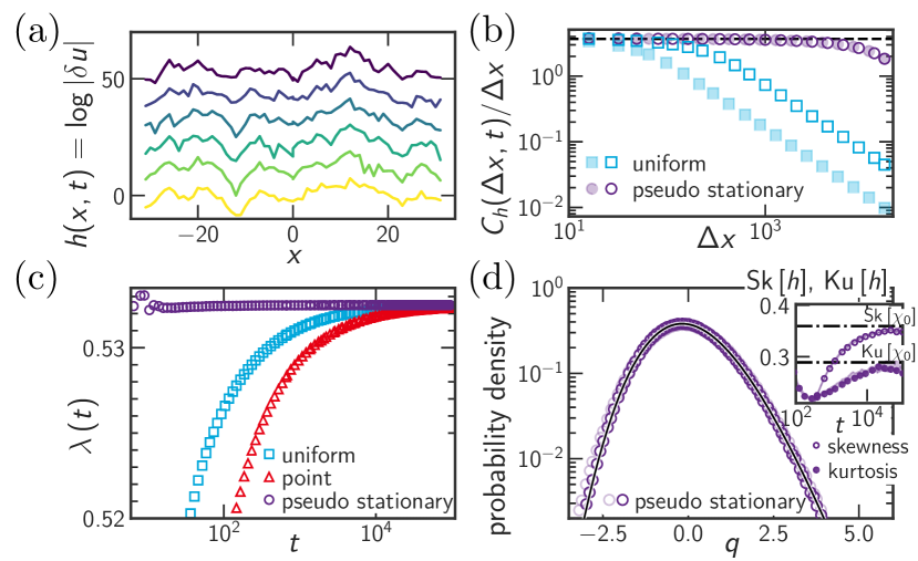
Figure 3: Results for the pseudo-stationary initial perturbations. (a) Typical snapshots of perturbation interfaces at $t=0,20,\cdots,100$ from bottom to top. (b) The height-difference correlation function $C_{h}(\Delta{}x,t)$ divided by $\Delta{}x$ at $t=10^{4}$ (lighter color) and $t=10^{5}$ (darker color). The dashed line shows the value of $A$. (c) The local Lyapunov exponent plotted against time. (d) The height distribution at $t=10^{3}$ (lighter color) and $t=10^{5}$ (darker color). The solid line shows the Baik-Rains distribution. (inset) The skewness and the kurtosis of $h(x,t)$. The shaded area indicates the systematic error due to the uncertainty of $A$ in $h_{0}(x)=\sqrt{A}B(x)$ (see text). The dash-dotted lines show the values for the Baik-Rains distribution.

V Convergence to the Lyapunov vector in finite-size systems

We have shown so far the initial-shape dependence of perturbation vectors, focusing on the three cases corresponding to the KPZ subclasses. On the other hand, for finite-size systems, we expect that the direction of the perturbation vectors eventually converges to that of the unique Lyapunov vector Eckmann and Ruelle (1985); Kuptsov and Parlitz (2012), whence the initial-condition dependence is lost. This is expected to happen when the correlation length $\xi(t)$ reaches the system size $L$. Here we investigated how this happens for the three studied initial perturbations, using the same system but with $L=2^{10}$. With this size, the correlation length $\xi(t)$ reaches $L$ at $t^{*}:=\Gamma^{-1}(\frac{AL}{2})^{3/2}\approx$6\text{\times}{10}^{5}$$.

To obtain the Lyapunov vector, we started simulations from $t=-T_{\mathrm{warmup}}-t_{0}$ with $t_{0}:=$6\text{\times}{10}^{6}$(\gg{}t^{*})$. After discarding the trajectory’s transient for $T_{\mathrm{warmup}}$ time steps, we applied a uniform perturbation $\delta{}u_{0}(x,-t_{0})=1$ and let it evolve for $t_{0}$ time steps. Then we defined $h_{\mathrm{stat}}(x,t):=\log\left|\delta{}u_{0}(x,t)\right|-\log\left|\delta{}u_{0}(0,0)\right|$, which is the interface corresponding to the Lyapunov vector and we call it the stationary perturbation interface. We compared it with the uniform, point, and pseudo-stationary interfaces $h(x,t)$ obtained for the same trajectory, and found that these indeed converge to $h_{\mathrm{stat}}(x,t)$ up to a constant shift which disappears by normalization of $\delta{}u(x,t)$ [Fig. 4(a)]. Interestingly, before this convergence, the difference $h(x,t)-h_{\mathrm{stat}}(x,t)$ consists of piece-wise plateaus, reminiscent of the difference between the first and subsequent Lyapunov vectors Pazó et al. (2008). The plateau edges meander in an apparently random manner, coalesce, and eventually annihilate [Fig. 4(b)].

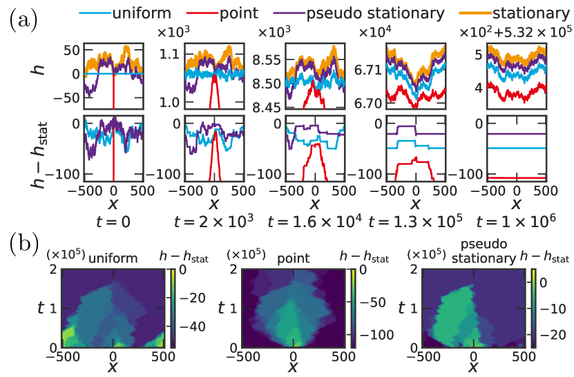
Figure 4: Convergence of the perturbation interfaces to the Lyapunov vector. (a) Typical snapshots, taken at time indicated below each panel, are shown. (b) Typical evolution of $h(x,t)-h_{\mathrm{stat}}(x,t)$.

VI Summary and discussion

In summary, using the logistic map CML as a prototypical model showing STC, we studied the distribution and correlation properties of perturbation vectors, for the following three types of initial perturbations: uniform, point, and pseudo-stationary. Focusing on the distribution and correlation properties, we showed clear evidence of agreement with the flat, circular, and stationary subclasses of the KPZ class, respectively. Since the KPZ exponents have been reported for perturbations in various STC systems Pikovsky and Kurths (1994); Pikovsky and Politi (1998); Pazó, López, and Politi (2013), it is reasonable to believe the generality of our results. In the pseudo-stationary case, the stationary KPZ subclass arises despite the fact that such a perturbation was not the Lyapunov vector and therefore not stationary for the dynamical system. These results indicate that the deterministic nature of dynamical systems does not affect the universal statistical properties of the KPZ class. When the correlation length eventually reaches the system size, the perturbation interfaces from different initial perturbations converged to the unique stationary interface up to constant shifts, unlike stochastic interface growth. This convergence is driven by intricate meandering, coalescence, and eventual annihilation of plateau borders seen in the height difference from the stationary interface.

Although we studied only the three types of initial perturbations here, the KPZ theory can also deal with general initial perturbations, via the KPZ variational formula Quastel and Remenik (2014); Corwin, Liu, and Wang (2016); Quastel and Remenik (2019); Fukai and Takeuchi (2020). We expect that we can describe the one-point distribution of perturbation vectors for arbitrary initial conditions, by using the numerical method proposed in Fukai and Takeuchi (2020) and by estimating nonuniversal parameters according to the procedure described in this article.

Recent studies have shown that the concept of the KPZ subclasses is also useful for understanding deterministic fluctuations of STC itself, in the Kuramoto-Sivashinsky equation Roy and Pandit (2020); Enrique Rodríguez-Fernández and Rodolfo Cuerno (2021), in anharmonic chains Mendl and Spohn (2016); Spohn (2016, 2017), in a discrete Gross-Pitaevskii equation Kulkarni, Huse, and Spohn (2015), etc. We hope that this line of research will continue providing new insights for spatially extended dynamical systems.

Supplementary Material

See supplementary material sup for Supplemental Texts on universal correlation functions and pseudo-stationary initial conditions, Table SI and Figs. S1, S2, S3, S4, S5 and S6.

Data Availability Statement

The data that support the findings of this study are openly available in Zenodo at https://doi.org/10.5281/zenodo.5559231.

References

- Pikovsky and Kurths (1994) A. S. Pikovsky and J. Kurths, “Roughening interfaces in the dynamics of perturbations of spatiotemporal chaos,” Phys. Rev. E 49, 898–901 (1994).
- Pikovsky and Politi (1998) A. Pikovsky and A. Politi, “Dynamic localization of Lyapunov vectors in spacetime chaos,” Nonlinearity 11, 1049 (1998).
- Kriecherbauer and Krug (2010) T. Kriecherbauer and J. Krug, “A pedestrian’s view on interacting particle systems, KPZ universality and random matrices,” J. Phys. A: Math. Theor. 43, 403001 (2010).
- Corwin (2012) I. Corwin, “The Kardar–Parisi–Zhang Equation and Universality Class,” Random Matrices Theory Appl. 01, 1130001 (2012).
- Quastel and Spohn (2015) J. Quastel and H. Spohn, “The One-Dimensional KPZ Equation and Its Universality Class,” J. Stat. Phys. 160, 965–984 (2015).
- Halpin-Healy and Takeuchi (2015) T. Halpin-Healy and K. A. Takeuchi, “A KPZ Cocktail-Shaken, not Stirred…” J. Stat. Phys. 160, 794–814 (2015).
- Sasamoto (2016) T. Sasamoto, “The 1D Kardar–Parisi–Zhang equation: Height distribution and universality,” Prog. Theor. Exp. Phys. 2016, 022A01 (2016).
- Spohn (2017) H. Spohn, “The Kardar–Parisi–Zhang equation: A statistical physics perspective,” in Stochastic Processes and Random Matrices: Lecture Notes of the Les Houches Summer School, Vol. 104, edited by G. Schehr, A. Altland, Y. V. Fyodorov, N. O’Connell, and L. F. Cugliandolo (Oxford University Press, Oxford, 2017) pp. 177–227.
- Takeuchi (2018) K. A. Takeuchi, “An appetizer to modern developments on the Kardar–Parisi–Zhang universality class,” Physica A 504, 77–105 (2018).
- Kaneko (1989) K. Kaneko, “Pattern dynamics in spatiotemporal chaos: Pattern selection, diffusion of defect and pattern competition intermettency,” Physica D 34, 1–41 (1989).
- Kaneko (1993) K. Kaneko, Theory and applications of coupled map lattices (Wiley, Chichester, New York, 1993).
- Oseledec (1968) V. I. Oseledec, “A multiplicative ergodic theorem. ljapunov characteristic numbers for dynamical systems,” Trans. Moscow Math. Soc. 19, 197–231 (1968).
- Eckmann and Ruelle (1985) J. P. Eckmann and D. Ruelle, “Ergodic theory of chaos and strange attractors,” Rev. Mod. Phys. 57, 617–656 (1985).
- Kuptsov and Parlitz (2012) P. V. Kuptsov and U. Parlitz, “Theory and Computation of Covariant Lyapunov Vectors,” J. Nonlinear Sci. 22, 727–762 (2012).
- Aranson and Kramer (2002) I. S. Aranson and L. Kramer, “The world of the complex ginzburg-landau equation,” Rev. Mod. Phys. 74, 99 (2002).
- Chaté and Manneville (1987) H. Chaté and P. Manneville, “Transition to turbulence via spatio-temporal intermittency,” Phys. Rev. Lett. 58, 112–115 (1987).
- Chaté and Manneville (1988) H. Chaté and P. Manneville, “Spatio-temporal intermittency in coupled map lattices,” Physica D 32, 409–422 (1988).
- Miller and Huse (1993) J. Miller and D. A. Huse, “Macroscopic equilibrium from microscopic irreversibility in a chaotic coupled-map lattice,” Phys. Rev. E 48, 2528–2535 (1993).
- Marcq, Chaté, and Manneville (1996) P. Marcq, H. Chaté, and P. Manneville, “Universal Critical Behavior in Two-Dimensional Coupled Map Lattices,” Phys. Rev. Lett. 77, 4003–4006 (1996).
- Marcq, Chaté, and Manneville (1997) P. Marcq, H. Chaté, and P. Manneville, “Universality in Ising-like phase transitions of lattices of coupled chaotic maps,” Phys. Rev. E 55, 2606–2627 (1997).
- Pikovsky, Rosenblum, and Kurths (2003) A. Pikovsky, M. Rosenblum, and J. Kurths, Synchronization: A Universal Concept in Nonlinear Sciences, Cambridge Nonlinear Science Series (Cambridge Univ. Press, New York, 2003).
- Ruelle (1982) D. Ruelle, “Large volume limit of the distribution of characteristic exponents in turbulence,” Commun. Math. Phys. 87, 287–302 (1982).
- Manneville (1985) P. Manneville, “Liapounov exponents for the Kuramoto-Sivashinsky model,” in Macroscopic Modelling of Turbulent Flows, Lecture Notes in Physics, edited by U. Frisch, J. B. Keller, G. C. Papanicolaou, and O. Pironneau (Springer, Berlin, Heidelberg, 1985) pp. 319–326.
- Egolf et al. (2000) D. A. Egolf, I. V. Melnikov, W. Pesch, and R. E. Ecke, “Mechanisms of extensive spatiotemporal chaos in Rayleigh–Bénard convection,” Nature 404, 733–736 (2000).
- Kardar, Parisi, and Zhang (1986) M. Kardar, G. Parisi, and Y.-C. Zhang, “Dynamic scaling of growing interfaces,” Phys. Rev. Lett. 56, 889 (1986).
- Spohn (2016) H. Spohn, “Fluctuating Hydrodynamics Approach to Equilibrium Time Correlations for Anharmonic Chains,” in Thermal Transport in Low Dimensions, Lecture Notes in Physics No. 921, edited by S. Lepri (Springer International Publishing, Cham, 2016) pp. 107–158.
- Ljubotina, Žnidarič, and Prosen (2019) M. Ljubotina, M. Žnidarič, and T. Prosen, “Kardar-parisi-zhang physics in the quantum heisenberg magnet,” Phys. Rev. Lett. 122, 210602 (2019).
- Scheie et al. (2021) A. Scheie, N. E. Sherman, M. Dupont, S. E. Nagler, M. B. Stone, G. E. Granroth, J. E. Moore, and D. A. Tennant, “Detection of kardar–parisi–zhang hydrodynamics in a quantum heisenberg spin-1/2 chain,” Nat. Phys. 17, 726–730 (2021).
- Wei et al. (2021) D. Wei, A. Rubio-Abadal, B. Ye, F. Machado, J. Kemp, K. Srakaew, S. Hollerith, J. Rui, S. Gopalakrishnan, N. Y. Yao, I. Bloch, and J. Zeiher, “Quantum gas microscopy of kardar-parisi-zhang superdiffusion,” (2021), arXiv:2107.00038 .
- Bulchandani, Gopalakrishnan, and Ilievski (2021) V. B. Bulchandani, S. Gopalakrishnan, and E. Ilievski, “Superdiffusion in spin chains,” (2021), arXiv:2103.01976 .
- Szendro et al. (2007) I. G. Szendro, D. Pazó, M. A. Rodríguez, and J. M. López, “Spatiotemporal structure of lyapunov vectors in chaotic coupled-map lattices,” Phys. Rev. E 76, 025202(R) (2007).
- Pazó et al. (2008) D. Pazó, I. G. Szendro, J. M. López, and M. A. Rodríguez, “Structure of characteristic Lyapunov vectors in spatiotemporal chaos,” Phys. Rev. E 78, 016209 (2008).
- Pazó, López, and Politi (2013) D. Pazó, J. M. López, and A. Politi, “Universal scaling of Lyapunov-exponent fluctuations in space-time chaos,” Phys. Rev. E 87, 062909 (2013).
- Pazó and López (2010) D. Pazó and J. M. López, “Characteristic Lyapunov vectors in chaotic time-delayed systems,” Phys. Rev. E 82, 056201 (2010).
- Prähofer and Spohn (2000) M. Prähofer and H. Spohn, “Statistical self-similarity of one-dimensional growth processes,” Physica A 279, 342–352 (2000).
- Takeuchi and Sano (2010) K. A. Takeuchi and M. Sano, “Universal Fluctuations of Growing Interfaces: Evidence in Turbulent Liquid Crystals,” Phys. Rev. Lett. 104, 230601 (2010).
- Takeuchi et al. (2011) K. A. Takeuchi, M. Sano, T. Sasamoto, and H. Spohn, “Growing interfaces uncover universal fluctuations behind scale invariance.” Sci. Rep. 1, 34 (2011).
- Takeuchi and Sano (2012) K. A. Takeuchi and M. Sano, “Evidence for Geometry-Dependent Universal Fluctuations of the Kardar-Parisi-Zhang Interfaces in Liquid-Crystal Turbulence,” J. Stat. Phys. 147, 853–890 (2012).
- Fukai and Takeuchi (2017) Y. T. Fukai and K. A. Takeuchi, “Kardar-Parisi-Zhang Interfaces with Inward Growth,” Phys. Rev. Lett. 119, 030602 (2017).
- Iwatsuka, Fukai, and Takeuchi (2020) T. Iwatsuka, Y. T. Fukai, and K. A. Takeuchi, “Direct Evidence for Universal Statistics of Stationary Kardar-Parisi-Zhang Interfaces,” Phys. Rev. Lett. 124, 250602 (2020).
- Fukai and Takeuchi (2020) Y. T. Fukai and K. A. Takeuchi, “Kardar-Parisi-Zhang Interfaces with Curved Initial Shapes and Variational Formula,” Phys. Rev. Lett. 124, 060601 (2020).
- Barabási and H. Eugene Stanley (1995) A.-L. Barabási and H. Eugene Stanley, Fractal Concepts in Surface Growth (Cambridge University Press, New York, NY, USA, 1995).
- Tracy and Widom (1996) C. A. Tracy and H. Widom, “On orthogonal and symplectic matrix ensembles,” Commun. Math. Phys. 177, 727–754 (1996).
- Tracy and Widom (1994) C. A. Tracy and H. Widom, “Level-spacing distributions and the Airy kernel,” Commun. Math. Phys. 159, 151–174 (1994).
- Baik and Rains (2000) J. Baik and E. M. Rains, “Limiting Distributions for a Polynuclear Growth Model with External Sources,” J. Stat. Phys. 100, 523–541 (2000).
- Prähofer and Spohn (2000) M. Prähofer and H. Spohn, “Universal Distributions for Growth Processes in 1+1 Dimensions and Random Matrices,” Phys. Rev. Lett. 84, 4882–4885 (2000).
- Note (1) Note , where is the standard GOE Tracy-Widom random variable Tracy and Widom (1996).
- Ferrari and Spohn (2016) P. L. Ferrari and H. Spohn, “On Time Correlations for KPZ Growth in One Dimension,” Symmetry Integrability Geom. Methods Appl. 12, 074 (2016).
- De Nardis, Le Doussal, and Takeuchi (2017) J. De Nardis, P. Le Doussal, and K. A. Takeuchi, “Memory and Universality in Interface Growth,” Phys. Rev. Lett. 118, 125701 (2017).
- Johansson (2019) K. Johansson, “The two-time distribution in geometric last-passage percolation,” Probab. Theory Related Fields 175, 849–895 (2019).
- Johansson and Rahman (2021) K. Johansson and M. Rahman, “Multitime distribution in discrete polynuclear growth,” Commun. Pure Appl. Math. (2021), 10.1002/cpa.21980.
- Liu (2019) Z. Liu, “Multi-point distribution of TASEP,” (2019), arXiv:1907.09876 .
- Corwin, Quastel, and Remenik (2015) I. Corwin, J. Quastel, and D. Remenik, “Renormalization Fixed Point of the KPZ Universality Class,” J. Stat. Phys. 160, 815–834 (2015).
- Dauvergne, Ortmann, and Virág (2019) D. Dauvergne, J. Ortmann, and B. Virág, “The directed landscape,” (2019), arXiv:1812.00309 .
- (55) See Supplemental Material for Supplemental Text, Table SI and Figs. S1, S2, S3, S4, S5 and S6, which includes Refs. Sasamoto (2005); Borodin et al. (2007); Prähofer and Spohn (2002); Baik, Ferrari, and Péché (2010).
- Krug, Meakin, and Halpin-Healy (1992) J. Krug, P. Meakin, and T. Halpin-Healy, “Amplitude universality for driven interfaces and directed polymers in random media,” Phys. Rev. A 45, 638–653 (1992).
- Ferrari and Frings (2011) P. L. Ferrari and R. Frings, “Finite Time Corrections in KPZ Growth Models,” J. Stat. Phys. 144, 1123 (2011).
- Prähofer and Spohn (2004) M. Prähofer and H. Spohn, “Exact Scaling Functions for One-Dimensional Stationary KPZ Growth,” J. Stat. Phys. 115, 255–279 (2004).
- Quastel and Remenik (2014) J. Quastel and D. Remenik, “Airy Processes and Variational Problems,” in Topics in Percolative and Disordered Systems (Springer, New York, NY, 2014) pp. 121–171.
- Corwin, Liu, and Wang (2016) I. Corwin, Z. Liu, and D. Wang, “Fluctuations of TASEP and LPP with general initial data,” Ann. Appl. Probab. 26, 2030–2082 (2016).
- Quastel and Remenik (2019) J. Quastel and D. Remenik, “How flat is flat in random interface growth?” Trans. Amer. Math. Soc. 371, 6047–6085 (2019).
- Roy and Pandit (2020) D. Roy and R. Pandit, “One-dimensional Kardar-Parisi-Zhang and Kuramoto-Sivashinsky universality class: Limit distributions,” Phys. Rev. E 101, 030103(R) (2020).
- Enrique Rodríguez-Fernández and Rodolfo Cuerno (2021) Enrique Rodríguez-Fernández and Rodolfo Cuerno, “Transition between chaotic and stochastic universality classes of kinetic roughening,” Physical Review Research 3, L012020 (2021).
- Mendl and Spohn (2016) C. B. Mendl and H. Spohn, “Searching for the tracy-widom distribution in nonequilibrium processes,” Phys. Rev. E 93, 060101(R) (2016).
- Kulkarni, Huse, and Spohn (2015) M. Kulkarni, D. A. Huse, and H. Spohn, “Fluctuating hydrodynamics for a discrete gross-pitaevskii equation: Mapping onto the kardar-parisi-zhang universality class,” Phys. Rev. A 92, 043612 (2015).
- (66) Theoretical curves available in the following URL were used: https://www-m5.ma.tum.de/KPZ.
- Bornemann (2010) F. Bornemann, “On the numerical evaluation of fredholm determinants,” Math. Comput. 79, 871–915 (2010).
- Sasamoto (2005) T. Sasamoto, “Spatial correlations of the 1D KPZ surface on a flat substrate,” J. Phys. A: Math. Gen. 38, L549 (2005).
- Borodin et al. (2007) A. Borodin, P. L. Ferrari, M. Prähofer, and T. Sasamoto, “Fluctuation Properties of the TASEP with Periodic Initial Configuration,” J. Stat. Phys. 129, 1055–1080 (2007).
- Prähofer and Spohn (2002) M. Prähofer and H. Spohn, “Scale Invariance of the PNG Droplet and the Airy Process,” J. Stat. Phys. 108, 1071–1106 (2002).
- Baik, Ferrari, and Péché (2010) J. Baik, P. L. Ferrari, and S. Péché, “Limit process of stationary TASEP near the characteristic line,” Commun. Pure Appl. Math. 63, 1017–1070 (2010).