Characterization of topological insulators based on the electronic polarization with spiral boundary conditions

Abstract

We introduce the electronic polarization originally defined in one-dimensional lattice systems to characterize two-dimensional topological insulators. The main idea is to use spiral boundary conditions which sweep all lattice sites in one-dimensional order. We find that the sign of the polarization changes at topological transition points of the two-dimensional Wilson-Dirac model (the lattice version of the Bernevig-Hughes-Zhang model) in the same way as in one-dimensional systems. Thus the polarization plays the role of “order parameter” to characterize the topological insulating state and enables us to study topological phases in different dimensions in a unified way.

Introduction. For more than ten years, topological phases and topological transitions have been extensively studied in connection with topological insulators [1, 2, 3, 4, 5, 6, 7]. Topological insulators have energy gaps in the bulk and gapless edge (surface) states in two (three) dimensions. On the other hand, topological phases and topological transitions have also been discussed in two-dimensional (2D) classical spin systems and one-dimensional (1D) quantum spin systems since the 1970s [8, 9, 10]. For example a dimer-Néel transition in a spin-$1/2$ frustrated anisotropic Heisenberg chain is regarded as a transition between two topologically distinct gapped phases [11]. The discovery of the Haldane gap in integer spin chains has added to the variety of topological phases [12, 13]. In this Research Letter, we study these topological phases and topological transitions of different systems in different dimensions in a unified way.

For this purpose, we consider the electronic polarization [14, 15, 16, 17, 18]. In 1D lattice electron systems, the polarization operator is defined as the following ground-state $\ket{\Psi_{0}}$ expectation value of the “twist operator” $U$,

$$z^{(q)}=\braket{\Psi_{0}}{U^{q}}{\Psi_{0}},\quad U=\exp\biggl{(}{\rm i}\frac{2\pi}{L}\sum_{j=1}^{L}jn_{j}\biggr{)}$$ (1)

where $L$ is the number of sites, $n_{j}$ is the electron number operator at $j$ th site, and $q$ is the degeneracy of the ground state. Resta related $z^{(1)}$ with the electronic polarization as $\lim_{L\to\infty}(e/2\pi){\rm Im}\;\!\ln z^{(1)}$ [15]. This quantity $z^{(q)}$ has been calculated for several 1D systems [16, 19, 20]. Hereinafter we call $z^{(q)}$ itself “polarization.” The signs of $z^{(q)}$ identify topologies of the systems such as charge or spin density waves. By replacing $n_{j}$ with a spin operator $S_{j}^{z}$, $z^{(q)}$ can also identify several magnetic orders including valence bond solid states [20]. Furthermore the condition $z^{(q)}=0$ can be used to detect a phase transition point.

The same quantity as in Eq. (1) was also introduced in the Lieb-Schultz-Mattis (LSM) theorem for 1D quantum systems [21, 22, 23, 24, 25]. In the LSM theorem, Eq. (1) appears as an overlap between the ground state and a variational excited state. According to the LSM theorem, an energy gap above a $q$-fold degenerate ground state is possible for $z^{(q)}\neq 0$ with $L\to\infty$.

Thus the property of the polarization $z^{(q)}$ has been well studied for 1D systems, however, its application to higher dimensional systems is not fully understood. In this Research Letter, we extend the twist operator in Eq. (1) to 2D systems, characterize the topological orders, and identify topological transition points. The main idea of our study is to use spiral boundary conditions (SBC) which sweep all lattice sites in one-dimensional orders. For a 2D square lattice with the number of lattices $L_{x}\times L_{y}$, SBC are introduced as shown in Fig. 1. These boundary conditions have been introduced in extending the LSM theorem to higher dimensions [26, 27] to remove unphysical restrictions for the system sizes [28]. We further introduce the parameter $\Lambda$ to deal with a variety of modulations. Then we show that topological insulating states in 2D systems can be identified by the polarization (1) with SBCs. Throughout this Research Letter, the lattice constant $a$ and the reduced Planck constant $\hbar$ are set to unity.

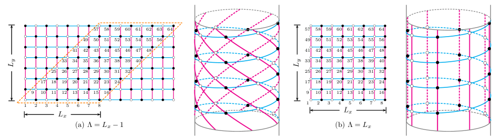
Figure 1: (a) and (b) Spiral boundary conditions (SBCs) for 2D square lattices where the systems are represented as extended 1D chains (blue lines). The parameter $\Lambda$ is the hopping range $c_{i+\Lambda,\alpha}^{{\dagger}}c_{i,\alpha}^{\mathstrut}+\mbox{H.c.}$ of the 1D chain originating from the hopping along the $y$ direction (magenta lines). For even $L_{x}$, $\bm{k}=(\pi,\pi)$ [$\bm{k}=(\pi,0)$] order is represented by 1D $k=\pi$ modulation with $\Lambda=L_{x}-1$ ($\Lambda=L_{x}$). For odd $L_{z}$, the roles of $\Lambda$ are interchanged.

The Wilson-Dirac model. As a fundamental model to describe 2D topological insulators, we consider the Wilson-Dirac model [29, 30], which is the lattice version of the Bernevig-Hughes-Zhang (BHZ) model [3, 4],

$$\mathcal{H}= \sum_{\bm{k},\alpha,\beta}c^{\dagger}_{\bm{k},\alpha}\,H_{\alpha\beta}(\bm{k})\,c^{\mathstrut}_{\bm{k},\beta},$$ (2a)

$$H(\bm{k})= t\sum_{\mu=x,y}\sin k_{\mu}\,\tau_{\mu}+\left[M-B\sum_{\mu=x,y}\bigl{(}1-\cos k_{\mu}\bigr{)}\right]\tau_{z},$$ (2b)

where $t$ is the hopping amplitude, $M$ is the mass, $B$ is the coefficient of the Wilson term, $c_{\bm{k},\alpha}$ is the annihilation operator of a fermion with a 2D wave number, $\alpha,\beta$ are orbital indices, and $\tau_{\mu}$ are the Pauli matrices. The energy eigenvalue is given by

$$\varepsilon_{\bm{k}}^{2}=t^{2}(\sin^{2}k_{x}+\sin^{2}k_{y})+\bigl{\{}M-B(2-\cos k_{x}-\cos k_{y})\bigr{\}}^{2}.$$ (3)

This system is a topological (trivial) insulator for $B<M/4$ ($B>M/4$), and a phase transition among two topological phases occurs at $B=M/2$. These transition points can be identified by vanishing of the bulk energy gap $\varepsilon_{\bm{k}}=0$. In the continuum version of the model, the Hall conductivity is calculated as [31]

$$\sigma_{xy}=-\frac{e^{2}}{2h}[{\rm sgn}(M)+{\rm sgn}(B)].$$ (4)

Therefore the system is a topological (trivial) insulator for $MB>0$ ($MB<0$), and a topological transition occurs at $B=0$ for fixed $M$.

Now we consider the lattice model (2) based on SBC. Here SBC are introduced by replacing the 2D wave vector $\bm{k}=(k_{x},k_{y})$ as $k_{x}\to k$ and $k_{y}\to\Lambda k$ with the 1D Fourier transformation

$$c_{k,\alpha}=\frac{1}{\sqrt{L}}\sum_{j=1}^{L}{\rm e}^{-{\rm i}kx_{j}}c_{j,\alpha},$$ (5)

where $L\equiv L_{x}L_{y}$, $x_{j}=aj$, and $k=2\pi n/L$ with $n=0,1,2,\cdots,L-1$ meaning periodic boundary conditions (PBCs) for the extended 1D chain, $c_{i+L,\alpha}=c_{i,\alpha}$. When $L_{x}$ is even, the parameter $\Lambda$ is chosen as $\Lambda=L_{x}-1$ [$\Lambda=L_{x}$] to detect a modulation of $\bm{k}=(\pi,\pi)$ [$\bm{k}=(0,\pi),(\pi,0)$] as shown in Fig. 1. The present system has translational symmetry $\mathcal{T}c_{j,\alpha}\mathcal{T}^{-1}=c_{j+1,\alpha}$ and parity symmetry $\mathcal{P}c_{j,\alpha}\mathcal{P}=c_{L-j+1,\alpha}$, so that $z^{(q)}=z^{(q)}{\rm e}^{-{\rm i}2q\pi N/L}$ and $z^{(q)}=[z^{(q)}]^{*}{\rm e}^{{\rm i}2q\pi N/L}$ with $N$ being the number of fermions. Thus we should choose $q=1$ in the present case with $N=L$.

Polarization. In order to calculate the polarization $z^{(1)}$ for the 2D Wilson-Dirac model, we use the following Resta’s argument [15]. After the inverse Fourier transformation, the Wilson-Dirac model (2) with SBCs is written as a 1D quadratic Hamiltonian [32],

$$\mathcal{H}=\sum_{ij,\alpha\beta}c_{i\alpha}^{\dagger}H_{ij,\alpha\beta}c_{j\beta}^{\mathstrut},$$ (6)

where $i,j$ are sites. Then we obtain its single-particle eigenstates by

$$\sum_{j^{\prime}}H_{jj^{\prime}}\ket{\psi^{j^{\prime}}_{p\mu}}=\varepsilon_{p\mu}\ket{\psi^{j}_{p\mu}},$$ (7)

where $\ket{\psi^{j}_{p\mu}}=\mathcal{U}^{-1}_{jp}\ket{u_{p\mu}}$, $\mathcal{U}^{\mathstrut}_{pj}={\rm e}^{-{\rm i}px_{j}}/\sqrt{L}$, and $\ket{u_{p\mu}}$ are the eigenstates of the Bloch Hamiltonian $H(p)=\sum_{jj^{\prime}}\mathcal{U}^{\mathstrut}_{pj}H_{jj^{\prime}}\mathcal{U}^{-1}_{j^{\prime}p}$. Then the polarization is given as

$$z^{(q)}={\rm det}^{\prime}S^{(q)},\quad S^{(q)}_{\mu,\nu}(k_{s},k_{s^{\prime}})=\sum_{j=1}^{L}\braket{\psi^{j}_{k_{s}\mu}}{{\rm e}^{{\rm i}\frac{2q\pi}{L}x_{j}}}{\psi^{j}_{k_{s^{\prime}}\nu}},$$ (8)

where det^′ indicates the determinant restricted to the occupied single-particle states. This calculation is simplified as

$${\rm det}\;S^{(q)}=(-1)^{q}\prod_{s=0}^{L-1}{\rm det}\;S^{(q)}(k_{s+q},k_{s}),$$ (9)

$$S^{(q)}_{\mu,\nu}(k_{s+q},k_{s})=\braket{u_{k_{s+q}\mu}}{u_{k_{s}\nu}},$$ (10)

where $k_{s}=2\pi s/L$, and the factor $(-1)^{q}$ stems from the antisymmetry of the determinant [32]. Here the meaning of the polarization becomes clear: it is a product of overlaps between Bloch states with wave vectors that differ by $k_{q}$. This decomposition to small matrices and cancellation of $x_{j}$ dependence greatly simplify the calculations and enable us to deal with large systems. Especially, in the present system with a single occupied band, $S_{\mu,\nu}(k_{s+1},k_{s})$ is no longer a matrix but a number. This simplification is also one of the advantages of SBCs where each state is specified by a single wave number $k$, compared with conventional 2D PBCs.

Conductivities. As a physical quantity to compare with the polarization, we calculate the Hall conductivity $\sigma_{xy}$ which is given in Matsubara form as

$${\rm Re}\;\sigma_{ij}=-\lim_{\omega\to 0}\frac{{\rm Im}\;\Pi_{ij}^{\rm R}(0,\omega)}{\omega}\qquad\{i,j\}\in\{x,y\}$$ (11a)

$$\Pi_{ij}(p,{\rm i}\nu_{m})=\frac{e^{2}}{L_{i}L_{j}\beta}\sum_{k,\omega_{n}}$$ (11b)

$$\times{\rm Tr}\left[\mathcal{G}(k,{\rm i}\omega_{n})\,\gamma_{i}\left(k+\tfrac{p}{2}\right)\mathcal{G}(k+p,{\rm i}\omega_{n}+{\rm i}\nu_{m})\,\gamma_{j}\left(k+\tfrac{p}{2}\right)\right]$$

where $\beta$ is the inverse temperature, and the temperature Green’s function is given as $\mathcal{G}(k,{\rm i}\omega_{n})=({\rm i}\omega_{n}-(H(k)-\mu)+{\rm i}\,{\rm sgn}(\omega_{n})\Gamma)^{-1}$ with $\omega_{n}$ and $\nu_{m}$ being Matsubara frequencies for fermions and bosons, respectively. The chemical potential and the impurity scattering time are denoted by $\mu(=0)$ and $1/2\Gamma$, respectively. $\gamma_{i}$ is defined by

$$\gamma_{i}(\bm{k})=\frac{\partial H(\bm{k})}{\partial k_{i}},$$ (12)

and the replacement of the wave number $(k_{x},k_{y})\to(k,\Lambda k)$ [32].

Results. First, we look at the dispersion relation of the 2D Wilson-Dirac model with SBCs as shown in Fig. 2. The Brillouin zone is $0\leq k<2\pi$. Since the present model with SBCs is represented as a 1D model with long-range hopping terms $c_{i+\Lambda,\alpha}^{{\dagger}}c_{i,\alpha}^{\mathstrut}+\mbox{H.c.}$, there appear many oscillations. At the phase transition points where the bulk gap closes, Dirac points appear at $k=\pi$ for $\Lambda=L_{x}-1$ and $\Lambda=L_{x}$. Here we have assumed that $L_{x}$ is even. For odd $L_{x}$, the roles of $\Lambda$ are interchanged.

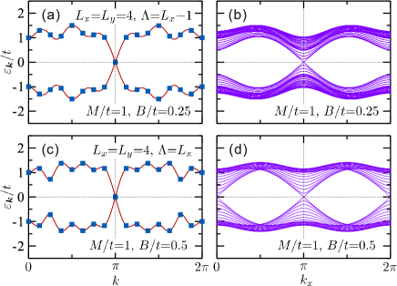
Figure 2: Dispersion relations of the 2D Wilson-Dirac model ($L_{x}=L_{y}=4$, $M/t=1$) at $B=M/4$ [(a) and (b)] and at $B=M/2$ [(c) and (d)]. (a) and (c) are written with spiral boundary conditions for $\Lambda=L_{x}-1$ and for $\Lambda=L_{x}$, respectively, while (b) and (d) are based on conventional 2D boundary conditions. The bulk gap closes and the Dirac dispersion appears at $k=\pi$.

We calculate several quantities including the polarization as shown in Fig. 3. As expected, the Hall conductivity at zero temperature vanishes ($\sigma_{xy}=0$) in the trivial phase $B<M/4$ and $\sigma_{xy}=\pm e^{2}/2h$ for the topological phase $B>M/4$ as shown in Fig. 3(a). This is due to the absence of chiral symmetry. At the phase transition between two topological states $B=M/2$, the sign of the Hall conductivity changes. The results of the lattice model do not coincide with those of the effective mass approximation. Since the Hall conductivity is defined in the thermodynamic limit, the results do not depend on boundary conditions: we get the same quantized Hall conductivities for SBC with $\Lambda=L_{x}-1$ and $\Lambda=L_{x}$, and also for the usual 2D PBCs. However, at the phase transition points, the Hall conductivity diverges because of the vanishing of the bulk energy gap $\varepsilon_{k}=0$. Therefore we have calculated the Hall conductivity in antiperiodic boundary conditions (APBCs) for the extended 1D chain, $c_{i+L,\alpha}=-c_{i,\alpha}$, namely $k=2\pi(n+1/2)/L$, to prevent these divergences.

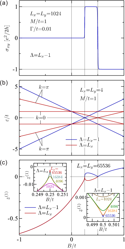
Figure 3: Several quantities around the parameter regions of the topological transitions of the 2D Wilson-Dirac model with $M/t=1$: (a) Hall conductivity, (b) energy levels in a finite-size system, and (c) polarization. The Hall conductivity is quantized at $\pm e^{2}/2h$. (a) and (c) are calculated under SBC with APBC $c_{i+L,\alpha}=-c_{i,\alpha}$ to prevent divergences at the transition points ($B/t=1/4,1/2$). The insets of (c) show how $z^{(1)}$ approaches to zero at the transition points. The polarizations with different $\Lambda$ converge to the same value except for the intermediate region $1/4<B/t<1/2$.

Next we consider energy spectra of the 2D Wilson-Dirac model in finite-size systems. As shown in Fig. 3(b), energies of $\bm{k}=(\pi,\pi)$ $[(k,\Lambda)=(\pi,L_{x}-1)]$ intersect at the topological phase transition point at $B=M/4$ without size dependence. This is similar to “level spectroscopy” for 1D quantum systems [33, 34, 35]. In this method, phase transition points between two different gapped states described by $c=1$ conformal field theory are identified by an intersection of energy spectra with different parities. The phase transition point at $B=M/2$ is also given by an intersection of energy spectra, but these spectra are given by $\bm{k}=(\pi,0)$ $[(k,\Lambda)=(\pi,L_{x})]$, so that we need to choose $\Lambda=L_{x}$.

Now we turn our attention to the polarization $z^{(1)}$ which is the main target of this Research Letter. Before looking at the result, let us evaluate the sign of $z^{(1)}$ from the real space representation of the 2D Wilson-Dirac model [32]. For the trivial phase ($B\ll 0\ll M$), the electrons of the system are located on each site; therefore it follows from $(2\pi/L)\sum_{j=1}^{L}j=(L+1)\pi$ that $z^{(1)}=-1$ for even $L$. On the other hand, the topological phase ($0\ll M\ll B$) is considered to be dominated by bond-located fermions. When all the fermions are located on the bonds along the $x$ direction, the wave function is $\ket{\Psi_{0}}=2^{-L/2}\prod_{k=1}^{L/2}(c_{2k-1,1}^{{\dagger}}+c_{2k,1}^{{\dagger}})(c_{2k,2}^{{\dagger}}+c_{2k+1,2}^{{\dagger}})\ket{0}$. Then the polarization is calculated as $z^{(1)}=[\cos(\pi/L)]^{L}{\rm e}^{{\rm i}(L+2)\pi}\to 1$ for $L\to\infty$. Here, the phase is given by the center of mass of the bond-located fermions $(2\pi/L)\sum_{j=1}^{L}(j+1/2)$. If there are bond-located fermions along the $y$ direction, then $\ket{\Psi_{0}}$ includes long range bonds $2^{-1/2}(c_{j,\alpha}^{{\dagger}}+c_{j+\Lambda,\alpha}^{{\dagger}})\ket{0}$ in the 1D representation. However, in such cases, the center of mass of the bond-located fermions is unchanged regardless of the choice of $\Lambda$ [32]. Therefore, the sign of $z^{(1)}$ is expected to change between the topological and the trivial phases.

As shown in Fig. 3(c), the sign of $z^{(1)}$ changes between the trivial and the topological regions, as we expected. For the region between two phase transition points at $B=M/4$ and $B=M/2$, the sign of $z^{(1)}$ becomes different depending on the choice of $\Lambda$. The interpretation of this result is not clear, but the difference in the sign of $z^{(1)}$ indicates the system given by bond-located fermions with modulations characterized by $(k_{x},k_{y})=(\pi,\pi)$ or $(\pi,0),(0,\pi)$. For even $L_{x}$, $z^{(1)}$ with $\Lambda=L_{x}-1$ changes the sign at $B=M/4$ and approaches to zero at $B=M/2$, while for $\Lambda=L_{x}$, $z^{(1)}$ approaches to zero at $B=M/4$ and changes the sign at $B=M/2$. The fact that $z^{(1)}$ vanishes at the phase transition points where the system is gapless is consistent with the LSM theorem. Here, we have used SBCs with APBCs $c_{i+L,\alpha}=-c_{i,\alpha}$ to prevent divergences at the transition points. For PBCs, $z^{(1)}$ changes discontinuously at the level-crossing point in finite-size systems [36].

Summary and discussion. In summary, we have discussed the polarization in the 2D Wilson-Dirac model based on spiral boundary conditions that sweep all lattice sites in 1D order. Here the system is described as 1D chains with long-range hopping. Then the electronic polarization defined in 1D systems can be extended to 2D systems. In the same way as in the 1D cases, topologically distinct gapped phases are characterized by the difference of the sign in the polarization. This means that the polarization operator and SBCs enable us to deal with topological transitions between different gapped states in different dimensions in a unified way.

The SBCs also have a great advantage in calculating the polarization. In Resta’s formalism for non-interacting systems, the polarization $z^{(q)}$ is given by products of overlaps between the Bloch states with wave vectors separated by $2q\pi/L$, so that denoting the states by 1D wave numbers greatly reduces the calculation costs, and enables us to obtain results in large enough systems to be almost regarded as the thermodynamic limit. The present SBCs are also useful for several numerical methods, such as the exact diagonalization and the density matrix renormalization group.

We have analyzed the 2D Wilson-Dirac model successfully based on SBC, but we can not conclude here whether the behavior of the polarization is universal or not in other models of 2D topological insulators. We need further systematic study of the general relationship between the polarization and topological phases in several symmetries and dimensions, including calculations of other physical quantities such as entanglement spectra. For example, there are several works relating the Chern number and the conventional type of 2D twist operators [37, 38]. It would also be interesting to apply the present analysis to multipole polarizations in higher-order topological insulators [39, 40, 41] and non-Hermitian systems.

Acknowledgments. The authors thank K. Imura and M. Oshikawa for discussions, and U. Nitzsche for technical assistance. M. N. acknowledges the Visiting Researcher’s Program of the Institute for Solid State Physics, The University of Tokyo, and the research fellow position of the Institute of Industrial Science, The University of Tokyo. M. N. is supported partly by MEXT/JSPS KAKENHI Grant Number JP20K03769. S. N. acknowledges support from SFB 1143 project A05 (project-id 247310070) of the Deutsche Forschungsgemeinschaft.

References

- [1] F. D. M. Haldane, Phys. Rev. Lett. 61, 2015 (1988).
- [2] C. L. Kane and E. J. Mele, Phys. Rev. Lett. 95, 146802 (2005).
- [3] B. A. Bernevig and S. C. Zhang, Phys. Rev. Lett. 96, 106802 (2006).
- [4] B. A. Bernevig, T. L. Hughes, and S. C. Zhang, Science 314, 1757 (2006).
- [5] S. Ryu, A. P. Schnyder, A. Furusaki, and A.W. Ludwig, New J. Phys. 12, 065010 (2010).
- [6] M. König, S. Wiedmann, C. Brüne, A. Roth, H. Buhmann, L. W. Molenkamp, X.-L. Qi, and S.-C. Zhang, Science, 318, 766 (2007).
- [7] M. König, H. Buhmann, L. W. Molenkamp, T. Hughes, C.-X. Liu, X.-L. Qi, and S.-C. Zhang, J. Phys. Soc. Jpn. 77, 031007 (2008).
- [8] V. L. Berezinskii, Sov. Phys. JETP 32, 493 (1971).
- [9] V. L. Berezinskii, Sov. Phys. JETP 34, 610 (1972).
- [10] J. M. Kosterlitz and D. J. Thouless, J. Phys. C: Solid State Phys. 6, 1181 (1973).
- [11] F. D. M. Haldane, Phys. Rev. B 25, 4925(R) (1982).
- [12] F. D. M. Haldane, Phys. Lett. A93, 464 (1983).
- [13] F. D. M. Haldane, Phys. Rev. Lett. 50, 1153 (1983).
- [14] R. Resta, Rev. Mod. Phys. 66, 899 (1994).
- [15] R. Resta, Phys. Rev. Lett. 80, 1800 (1998).
- [16] R. Resta and S. Sorella, Phys. Rev. Lett. 82, 370 (1999).
- [17] R. Resta, J. Phys. Condens. Matter 12, R107 (2000).
- [18] A. A. Aligia and G. Ortiz, Phys. Rev. Lett. 82, 2560 (1999).
- [19] M. Nakamura and J. Voit, Phys. Rev. B 65, 153110 (2002).
- [20] M. Nakamura and S. Todo, Phys. Rev. Lett. 89, 077204 (2002).
- [21] E. Lieb, T. Schultz, and D. Mattis, Ann. Phys. (Amsterdam) 16, 407 (1961).
- [22] I. Affleck and E. H. Lieb, Lett. Math. Phys. 12, 57 (1986).
- [23] I. Affleck, Phys. Rev. B 37, 5186 (1988).
- [24] M. Oshikawa, M. Yamanaka, and I. Affleck, Phys. Rev. Lett. 78, 1984 (1997).
- [25] M. Yamanaka, M. Oshikawa, and I. Affleck, Phys. Rev. Lett. 79, 1110 (1997).
- [26] M. Oshikawa, Phys. Rev. Lett. 84, 1535 (2000).
- [27] M. B. Hastings, Europhys. Lett. 70, 824 (2005).
- [28] Y. Yao and M. Oshikawa, Phys. Rev. X 10, 031008 (2020).
- [29] K. G. Wilson, Phys. Rev. D 10, 2445 (1974).
- [30] X. L. Qi, Y. S. Wu, and S. C. Zhang, Phys. Rev. B 74, 085308 (2006).
- [31] H. So, Prog. Theor. Phys. 73, 528 (1985).
- [32] See Supplemental Material for details of calculations.
- [33] K. Okamoto and K. Nomura, Phys. Lett. A 169, 433 (1992).
- [34] K. Nomura and K. Okamoto, J. Phys. A: Math. Gen. 27, 5773 (1994).
- [35] A. Kitazawa, J. Phys. A: Math. Gen. 30, L285 (1997).
- [36] M. Nakamura and S. C. Furuya, Phys. Rev. B 99, 075128 (2019).
- [37] S. Coh and D. Vanderbilt, Phys. Rev. Lett. 102, 107603 (2009).
- [38] B. Kang, W. Lee, and G. Y. Cho, Phys. Rev. Lett. 126, 016402 (2021).
- [39] B. Kang, K. Shiozaki, and G. Y. Cho, Phys. Rev. B 100, 245134 (2019).
- [40] W. A. Wheeler, L. K. Wagner, and T. L. Hughes, Phys. Rev. B 100, 245135 (2019).
- [41] H. Watanabe and S. Ono, Phys. Rev. B 102, 165120 (2020).