Predictive Distributions and the Transition from Sparse to Dense Functional Data

Abstract

A representation of Gaussian distributed sparsely sampled longitudinal data in terms of predictive distributions for their functional principal component scores (FPCs) maps available data for each subject to a multivariate Gaussian predictive distribution. Of special interest is the case where the number of observations per subject increases in the transition from sparse (longitudinal) to dense (functional) sampling of underlying stochastic processes. We study the convergence of the predicted scores given noisy longitudinal observations towards the true but unobservable FPCs, and under Gaussianity demonstrate the shrinkage of the entire predictive distribution towards a point mass located at the true FPCs and also extensions to the shrinkage of functional $K$-truncated predictive distributions when the truncation point $K=K(n)$ diverges with sample size $n$. To address the problem of non-consistency of point predictions, we construct predictive distributions aimed at predicting outcomes for the case of sparsely sampled longitudinal predictors in functional linear models and derive asymptotic rates of convergence for the $2$-Wasserstein metric between true and estimated predictive distributions. Predictive distributions are illustrated for longitudinal data from the Baltimore Longitudinal Study of Aging.

Key words and phrases: Functional Data Analysis; Functional Principal Components; Wasserstein Metric; Sparse Design; Sparse-to-Dense; Baltimore Longitudinal Study of Aging.

1 Introduction

Functional Data Analysis (FDA) has found a wide range of applications (Horvath and Kokoszka, 2012; Wang et al., 2016), including the area of longitudinal studies, where functional principal component analysis (FPCA), a core technique of FDA, was shown to play an important role. A key feature of such studies is the sparsity of the available observations per subject, which are inherently correlated and are often available at only a few irregular times and may be contaminated with measurement error. In this case underlying random trajectories are latent and must be inferred from available data. Functional Principal Component Analysis (FPCA) (Kleffe, 1973; Castro et al., 1986) was found to be a key tool in this endeavour (Yao et al., 2005a).

When subjects are recorded densely over time, one can consistently recover the underlying random trajectories from the Karhunen–Loève representation that underpins FPCA, where a common approach is to employ Riemann sums to recover the integrals that correspond to projections of the trajectories on the eigenfunctions of the auto-covariance operator of the underlying stochastic process. These integrals correspond to the functional principal components (FPCs) and their approximation by Riemann sums improves as the number of observations per subject increases (Müller, 2005). However, when functional data are sparsely observed over time with noisy measurements, which is the quintessential scenario for longitudinal studies, one faces the challenge that simple Riemann sums do not converge, due to the low number of support points.

In response to this challenge, Yao et al. (2005a) introduced the Principal Analysis through Conditional Expectation (PACE) approach, which aims to recover the underlying trajectories by targeting the best prediction of the FPCs conditional on the observations, a quantity that can be consistently estimated based on consistent estimates of mean and covariance functions. These nonparametric estimates are obtained by pooling all observations across subjects, borrowing strength from the entire sample. While these predicted FPCs are unbiased, they have non-vanishing variance in the sparse case and thus do not lead to consistent trajectory recovery.

A second scenario where consistent predictions are unavailable in the sparse case is the Functional Linear Regression Model (FLM) for the relationship between a scalar or functional response $Y$ and functional predictors $X(t)\,t\in\mathcal{T}$, a compact interval (Ramsay and Silverman, 2005; Hall and Horowitz, 2007; Shi and Choi, 2011; Kneip et al., 2016; Chiou et al., 2016),

$$E[Y|X]=\mu_{Y}+\int_{\mathcal{T}}\beta(t)X^{c}(t)dt.$$ (1)

Here $\mu_{Y}=E(Y)$, $X^{c}(t)=X(t)-E(X(t))$ and the slope function $\beta$ lies in $L^{2}(\mathcal{T})$. It is a direct extension of the standard linear regression model to the case where the predictors lie in an infinite-dimensional space, usually assumed to be the Hilbert space $L^{2}(\mathcal{T})$.

To obtain a consistent estimate of the slope function $\beta$ in the FLM with sparse observations, it is well known that one can use the fact that the linear model structure allows to express the slope in terms of the cross covariance and covariance functions of the predictor process $X$ and the response, which are quantities that can be consistently estimated under mild assumptions (Yao et al., 2005b). Alternative multiple imputation methods based on conditioning on both the predictor observations and the response $Y$ have also been explored (Petrovich et al., 2018), and these also rely on cross-covariance estimation. However, these consistent estimates of the slope parameter function $\beta$ are not accompanied by consistent predictions, i.e. consistent estimates of $E[Y|X]$. This is because the integral in (1) cannot be consistently estimated even if $\beta$ is known, due to the sparse sampling of $X$, and poses a challenge for sparsely sampled predictors.

Our aim is to address these challenges by rephrasing the prediction of trajectories in the FPCA case and of scalar outcomes in the FLM case as predictive distribution problems. To implement this program, we study a map from sparse and irregularly sampled data to a multivariate Gaussian predictive distribution and then investigate the behavior of the estimated functional principal components (FPCs) as the number of observations per subject increases. We quantify the accompanying shrinkage of the conditional predictive distributions given the data and their convergence towards a point mass located at the true but unobserved FPCs.

For predicting the expected response $E[Y|X]$ in the FLM (1) in the sparse case, we also resort to constructing predictive distributions for the expected response given the information available for a subject. We show that these predictive distributions can be consistently estimated in the Wasserstein and Kolmogorov metric, and introduce a Wasserstein discrepancy measure to assess the predictability of the response by the predictive distribution. This measure is interpretable and can be consistently recovered under mild assumptions. Simulations support the utility of the Wasserstein discrepancy measure under different sparsity designs and noise levels. The predictive distribution are shown to converge towards the predictable truncated component of the response when transitioning from sparse to dense sampling.

2 Convergence of Predicted Functional Principal Components When Transitioning from Sparse to Dense Sampling

Assume that for each individual $i=1,\dots,n$, there is an underlying unobserved function $X_{i}(t)$, where the functions $X_{i}$ are i.i.d. realizations of a $L^{2}$-stochastic process $X(t),\,t\in\mathcal{T}$, and $\mathcal{T}$ is a closed and bounded interval on the real line. Without loss of generality we assume $\mathcal{T}=[0,1]$. Sparsely sampled and error-contaminated observations $\tilde{X}_{ij}=X_{i}(T_{ij})+\epsilon_{ij}$, $j=1,\dots,n_{i}$, are obtained at random times $T_{ij}\in\mathcal{T}$ that are distributed according to a continuous smooth distribution $F_{T}$. We require the following condition:

1. $\{T_{ij}:i=1,\dots,n,\,j=1,\dots,n_{i}\}$ are i.i.d. copies of a random variable $T$ defined on $\mathcal{T}$, and $n_{i}$ are regarded as fixed. The density $f(\cdot)$ of $T$ is bounded below, $\min_{t\in\mathcal{T}}f(t)\geq m_{f}>0$.

Assumption (S1) is a standard assumption (Zhang and Wang, 2016; Dai et al., 2018) to ensure there are no systematic sampling gaps. The measurement errors $\epsilon_{ij}$ are assumed to be i.i.d. Gaussian with mean 0 and variance $\sigma^{2}$, and independent of the underlying process $X_{i}(\cdot)$. Our analysis is conditional on the random number of observations per subject $n_{i}$ (Zhang and Wang, 2016). Denote the auto-covariance function of the process $X$ by

$$\Gamma(s,t) =\,\text{cov}(X(s),X(t))=\sum_{k=1}^{\infty}\lambda_{k}\phi_{k}(s)\phi_{k}(t),\quad s,t\in\mathcal{T},$$

where $\lambda_{1}>\lambda_{2}>\dots\geq 0$ are the ordered eigenvalues which satisfy $\sum_{k=1}^{\infty}\lambda_{k}<\infty$, and $\phi_{k}$, $k\geq 1$, are the orthonormal eigenfunctions associated with the Hilbert–Schmidt operator $\Xi(g)=\int_{\mathcal{T}}\Gamma(\cdot,t)g(t)dt$, $g\in L^{2}(\mathcal{T})$. Define eigengaps $\delta_{k}=\min(\lambda_{k-1}-\lambda_{k},\lambda_{k}-\lambda_{k+1})$, $k=1,2,\dots$, and denote by $\mu(t)=E(X_{i}(t))$ the mean function, $X_{i}^{c}(t)=X_{i}(t)-\mu(t)$ the centered process, and by $\xi_{ik}=\int_{\mathcal{T}}X_{i}^{c}(t)\phi_{k}(t)d{t}$ the $k$th functional principal component score (FPC), $k=1,2,\dots$. The FPCs satisfy $E(\xi_{ik})=0$, $E(\xi_{ik}^{2})=\lambda_{k}$ and $E(\xi_{ik}\xi_{il})=0$ for $k,l=1,2,\dots$ with $l\neq k$. Trajectories can then be represented through the Karhunen–Loève decomposition $X_{i}(t)=\mu(t)+\sum_{k=1}^{\infty}\xi_{ik}\phi_{k}(t)$, where in practice it is often useful to consider a truncated expansion using the first $K>0$ components that explain most of the variation, for example through the fraction of variance explained (FVE) criterion (Yao et al., 2005a). Denote by $\mathbf{T}_{i}=(T_{i1},\dots,T_{in_{i}})^{T}$ the sampling time points for the $i$th subject. Writing $\mathbf{X}_{i}=(\tilde{X}_{i1},\dots,\tilde{X}_{in_{i}})^{T}$ and conditional on $\mathbf{T}_{i}$, it follows that $\,\text{cov}(\tilde{X}_{ij},\xi_{ik}|\mathbf{T}_{i})=\lambda_{k}\phi_{k}(T_{ij})$, $j=1,\dots,n_{i}$ and $k=1,\dots,K$. Define

$$\bm{\Phi}_{iK}=\begin{pmatrix}\phi_{1}(T_{i1})&\dots&\phi_{K}(T_{i1})\\ \vdots&\vdots&\vdots\\ \phi_{1}(T_{in_{i}})&\dots&\phi_{K}(T_{in_{i}})\end{pmatrix},$$

$\bm{\mu}_{i}=\,\text{E}(\mathbf{X}_{i}|\mathbf{T}_{i})=(\mu(T_{i1}),\dots,\mu(T_{in_{i}}))^{T}$ and the $n_{i}\times n_{i}$ conditional covariance matrix $\bm{\Sigma}_{i}=\,\text{cov}(\mathbf{X}_{i}|\mathbf{T}_{i})$, for which the $(j,l)$ entry is given by $\sigma^{2}\delta_{jl}+\Gamma(T_{ij},T_{il})$, where $\delta_{jl}=1$ if $j=l$ and 0 otherwise. To predict the FPCs $\bm{\xi}_{iK}=(\xi_{i1},\xi_{i2},\dots,\xi_{iK})^{T}$, we utilize best linear unbiased predictors (BLUP) (Rice and Wu, 2001) of $\bm{\xi}_{iK}$ given $\mathbf{X}_{i}$ and $\mathbf{T}_{i}$, which are $\tilde{\bm{\xi}}_{iK}=\bm{\Lambda}_{K}\bm{\Phi}_{iK}^{T}\bm{\Sigma}_{i}^{-1}(\mathbf{X}_{i}-\bm{\mu}_{i})$, where $\bm{\Lambda}_{K}=\,\text{diag}(\lambda_{1},\dots,\lambda_{K})$.

We now show that as the number of observations for an individual increases as the functional sampling gets denser, the predicted FPCs $\tilde{\bm{\xi}}_{iK}$ converge to the true FPCs $\bm{\xi}_{iK}$, so that the true trajectory can be consistently recovered in the limit, under the following assumptions.

1. The process $X(t)$ is continuously differentiable a.s.  for $t\in\mathcal{T}$.

2. $\partial\Gamma(s,t)/\partial s$ exists and is continuous, for $s,t\in\mathcal{T}$.

Assumptions (S2)–(S3) are requirements for the smoothness of the original process and the covariance function, respectively. The following result does not require Gaussian assumptions.

Proposition 1.

Suppose that (S1)–(S3) hold and the number of observations $n_{i}$ for the $i$th subject satisfies $n_{i}=m\to\infty$, $i=1,\dots,n$. Then, for any fixed $K\geq 1$, $k=1,\dots,K$, and $i=1,\dots,n$, as $m\rightarrow\infty$ we have

$$|\tilde{\xi}_{ik}-\xi_{ik}| =O_{p}(m^{-1/2}).$$ (2)

This is the same rate of convergence as derived previously in Dai et al. (2018) for the FPCs of the derivative process $X^{\prime}(t)$ under Gaussian assumptions. This previous analysis utilized convergence results for nonparametric posterior distributions (Shen, 2002) that are tied to the Gaussian assumption, whereas here we develop a novel direct approach that does not require distributional assumptions on $X$. We next study scenarios where the unknown population quantities are estimated from the available data, where either the subjects are observed on dense designs, with $n_{i}=m\to\infty$, or on sparse designs, with $n_{i}\leq N_{0}<\infty$ for a fixed number $N_{0}<\infty$, reflecting few and irregularly timed observations per subject. To simplify notations, we will throughout use the following abbreviations for rates of convergence for the mean and covariance of the underlying stochastic process $X$,

$$a_{n1} =h_{\mu}^{2}+\left\{\frac{\log(n)}{nh_{\mu}}\right\}^{1/2},\quad b_{n1}=h_{G}^{2}+\left\{\frac{\log(n)}{nh_{G}^{2}}\right\}^{1/2},$$

$$a_{n2} =h_{\mu}^{2}+\left\{\left(1+\frac{1}{mh_{\mu}}\right)\frac{\log(n)}{n}\right\}^{1/2},\quad b_{n2}=h_{G}^{2}+\left(1+\frac{1}{mh_{G}}\right)\left\{\frac{\log(n)}{n}\right\}^{1/2},$$ (3)

where $h_{\mu}$ and $h_{G}$ are bandwidths. Quantities $a_{n}$ and $b_{n}$ will be used in the following in dependence on the design setting as follows: For sparse designs, $a_{n}=a_{n1}$ and $b_{n}=b_{n1}$, while for dense designs, $a_{n}=a_{n2}$ and $b_{n}=b_{n2}$.

The estimation of mean function $\mu$ and covariance surface $\Gamma$ is achieved through local linear smoothers analogously as in Zhang and Wang (2016), with further details in Section S.0 of the supplement. For the covariance smoothing step $n_{i}\geq 2$ is assumed throughout as in Zhang and Wang (2016). The estimation of remaining population quantities such as $\sigma^{2}$ and eigenpairs $(\lambda_{k},\phi_{k})$, $k\geq 1$, is carried out analogously as in equations $(2)$ and $(3)$ in Yao et al. (2005a). Denote by $\hat{\Xi}$ the estimated counterpart of the Hilbert–Schmidt integral operator $\Xi$ with eigenpairs $(\hat{\lambda}_{k},\hat{\phi}_{k})$ such that $\langle\hat{\phi}_{k},\phi_{k}\rangle_{L^{2}}\geq 0$, where $\langle\cdot,\cdot\rangle_{L^{2}}$ denotes the $L^{2}$ inner product and $k\geq 1$.

We show next that the estimated FPCs for a new independent subject $i^{*}$ that is not part of the training data sample ($i=1,\dots,n$), but for which measurements are available over a dense but possibly irregular grid, converge to the true FPCs, irrespective of whether the subjects in the training set are observed under sparse or dense designs. Specifically, given an independent realization $X^{*}$ of the process $X$, and independent of $X_{1},\dots,X_{n}$, we observe the measurements of the process $X^{*}$ made at times $T_{j}^{*}$ ($j=1,\dots,m^{*})$ with added noise, $\mathbf{X}^{*}=(X^{*}(T_{1}^{*})+\epsilon_{1}^{*},\dots,X^{*}(T_{m^{*}}^{*})+\epsilon_{m^{*}}^{*})$, where the errors $\epsilon_{j}^{*}$ are Gaussian with mean zero and variance $\sigma^{2}$, and independent of all other random quantities. The new independent subject is observed over $m^{*}\to\infty$ time points which may differ from the number $m$ of individual observations that is available under dense design settings for the training data. In the following, we consider the Karhunen–Loève decomposition $X^{*}(t)=\mu(t)+\sum_{k=1}^{\infty}\xi_{k}^{*}\phi_{k}(t)$ and the FPC score estimates $\hat{\xi}_{k}^{*}=\hat{\lambda}_{k}\hat{\phi}_{k}(\mathbf{T}^{*})^{T}\hat{\bm{\Sigma}}^{*-1}(\mathbf{X}^{*}-\hat{\bm{\mu}}^{*})$, where $\hat{\bm{\mu}}^{*}=\hat{\mu}(\mathbf{T}^{*}):=(\hat{\mu}(T_{1}^{*}),\dots,\hat{\mu}(T_{m^{*}}^{*}))^{T}$, $\hat{\phi}_{k}(\mathbf{T}^{*})=(\hat{\phi}_{k}(T_{1}^{*}),\dots,\hat{\phi}_{k}(T_{m^{*}}^{*}))^{T}$, $\mathbf{T}^{*}=(T_{1}^{*},\dots,T_{m^{*}}^{*})^{T}$, and $\hat{\bm{\Sigma}}^{*-1}$ is analogous to $\bm{\Sigma}_{i}^{-1}$ but replacing the $T_{ij}$ with $T_{j}^{*}$ and the population quantities by their estimated counterparts. We require that

1. The eigenvalues $\lambda_{1}>\lambda_{2}>\dots>0$ are all distinct.

The following result does not require Gaussianity of $X$.

Theorem 1.

Suppose that assumptions (S2), (B1) and (A1)–(A8) in the Appendix are satisfied. Consider either a sparse design setting when $n_{i}\leq N_{0}<\infty$ or a dense design when $n_{i}=m\to\infty$, $i=1,\dots,n$. Set $a_{n}=a_{n1}$ and $b_{n}=b_{n1}$ for the sparse case, and $a_{n}=a_{n2}$ and $b_{n}=b_{n2}$ for the dense case. For a new independent subject $i^{*}$ and $k\geq 1$, if $m^{*}(a_{n}+b_{n})=o(1)$ as $n\rightarrow\infty$, where $m^{*}=m^{*}(n)\to\infty$,

$$|\hat{\xi}_{k}^{*}-\xi_{k}^{*}|=O_{p}(m^{*-1/2}+m^{*}(a_{n}+b_{n})).$$

Further details on the rate of convergence are in the supplement, where it is shown that under certain choices of $m^{*}$ and bandwidths along with suitable regularity conditions one can obtain a rate arbitrarily close to $O_{p}((\log n/n)^{1/6})$ for sparse designs and to $O_{p}((\log n/n)^{1/2})$ for dense designs.

3 Predictive Distributions and the Transition from Sparse to Dense Sampling for Gaussian Processes

Consider the case when $X(t),\,t\in\mathcal{T},$ is a Gaussian process, so that $\bm{\xi}_{iK}=(\xi_{i1},\xi_{i2},\dots,\xi_{iK})^{T}\sim\textit{N}(0,\bm{\Lambda}_{K})$, where $K$ is a positive integer that corresponds to a truncation parameter. Conditional on $\mathbf{T}_{i}$, it follows that $\bm{\xi}_{iK}$ and $\mathbf{X}_{i}$ are jointly normal

$$\left(\begin{array}[]{c}\mathbf{X}_{i}\\ \bm{\xi}_{iK}\end{array}\right)\sim N\left(\left(\begin{array}[]{c}\bm{\mu}_{i}\\ 0\end{array}\right),\left(\begin{array}[]{cc}\bm{\Sigma}_{i}&\bm{\Phi}_{iK}\bm{\Lambda}_{K}\\ \bm{\Lambda}_{K}\bm{\Phi}_{iK}^{T}&\bm{\Lambda}_{K}\end{array}\right)\right),$$

and by a property of multivariate normal distributions (see for example Mardia et al. (1979)),

$$\bm{\xi}_{iK}|\mathbf{X}_{i},\mathbf{T}_{i}\sim N_{K}(\tilde{\bm{\xi}}_{iK},\bm{\Sigma}_{iK}),$$ (4)

where $\tilde{\bm{\xi}}_{iK}=E(\bm{\xi}_{iK}|\mathbf{X}_{i},\mathbf{T}_{i})=\bm{\Lambda}_{K}\bm{\Phi}_{iK}^{T}\bm{\Sigma}_{i}^{-1}(\mathbf{X}_{i}-\bm{\mu}_{i})$ is the best linear unbiased predictor (BLUP) of $\bm{\xi}_{iK}$ given $\mathbf{X}_{i}$ and $\mathbf{T}_{i}$, and $\bm{\Sigma}_{iK}=\bm{\Lambda}_{K}-\bm{\Lambda}_{K}\bm{\Phi}_{iK}^{T}\bm{\Sigma}_{i}^{-1}\bm{\Phi}_{iK}\bm{\Lambda}_{K}$ is the conditional variance. The relation in (4) was previously exploited, for example in Yao et al. (2005a), to construct simultaneous confidence bands for estimated trajectories; compare also Wang and Shi (2014). We refer to the conditional distribution in (4) as $K$-truncated predictive distribution since it is a distributional representation for the subject’s truncated true but unobserved scores $\bm{\xi}_{iK}$.

Note that (2) implies that the center of the $K$-truncated predictive distribution converges to the true FPCs $\bm{\xi}_{iK}$ in the transition from sparse to dense functional data. We now show that the entire $K$-truncated predictive distribution shrinks to a point mass located at its true $K$-truncated FPCs. Recall that $\bm{\Sigma}_{iK}$ is the conditional covariance as in (4) and for a matrix $A\in\mathbb{R}^{p\times q}$ denote by $\lVert A\rVert_{\text{op},2}=\sup_{\rVert v\rVert_{2}=1}\lVert Av\rVert_{2}$ the $2$-matrix norm, where $\lVert\cdot\rVert_{2}$ is the Euclidean norm in $\mathbb{R}^{p}$, $p,q>0$. For the following, we require Gaussianity.

1. The process $X(t)$, $t\in\mathcal{T}$, is Gaussian.

Proposition 2.

Suppose that (S1)–(S4) hold and the number of observations for the $i$th subject diverges, namely $n_{i}=m\to\infty$, $i=1,\dots,n$. Then, for any fixed $K\geq 1$ and $i=1,\dots,n$, as $m\rightarrow\infty$

$$\lVert\bm{\Sigma}_{iK}\rVert_{\text{op},2} =O_{p}(m^{-1}).$$

We note that Gaussianity is used only to derive the explicit form of the conditional covariance $\bm{\Sigma}_{iK}$ of the FPCs given the data $(\mathbf{X}_{i},\mathbf{T}_{i})$, which in this case does not depend on $\mathbf{X}_{i}$. If Gaussianity does not hold, using the explicit form of $E(\bm{\xi}_{iK}|\mathbf{X}_{i},\mathbf{T}_{i})$ in Section 2 and the relation $\,\text{var}(\bm{\xi}_{iK}\mid\mathbf{T}_{i})=\bm{\Lambda}_{K}$, by a conditioning argument $\bm{\Sigma}_{iK}\coloneqq E[\,\text{var}(\bm{\xi}_{iK}|\mathbf{X}_{i},\mathbf{T}_{i})\mid\mathbf{T}_{i}]=\,\text{var}(\bm{\xi}_{iK}\mid\mathbf{T}_{i})-\,\text{var}(E(\bm{\xi}_{iK}|\mathbf{X}_{i},\mathbf{T}_{i})\mid\mathbf{T}_{i})$ share the same definition as in the Gaussian case, and Proposition 2 continues to hold for this $\bm{\Sigma}_{iK}$.

Propositions 1 and 2 show that the $K$-truncated predictive distribution of a given subject shrinks to the true $K$-truncated FPCs $\bm{\xi}_{iK}$ at a root-$m$ rate as the number of observations per subject diverges. As detailed in Theorem S7 in the Supplement, the estimated covariance $\hat{\bm{\Sigma}}_{K}^{*}$ for an independent subject $i^{*}$ as in Section 2, and thus its $K$-truncated predictive distribution can be consistently recovered. Figure 1 displays the $95\%$ contours for $10$ predictive distributions for a given subject when varying the number of observations in the transition from sparse to dense: $n_{i}=2$ (very sparse; left panel), $n_{i}=10$ (medium sparse; middle panel), and $n_{i}=50$ (dense; right panel). Here we set $K=2$, $\sigma=0.5$, $\phi_{1}(t)=-\cos(\pi t/10)/\sqrt{5}$, $\phi_{2}(t)=\sin(\pi t/10)/\sqrt{5}$, $\mu(t)=t+\sin(t)$, $t\in\mathcal{T}=[0,10]$, and the time points are sampled from a uniform distribution on $\mathcal{T}$. As expected, the predictive distributions shrink towards a point mass located at the true unobserved subject FPCs (black dot) as the data gets denser. Since the entire trajectory can be recovered from the FPC scores, a distributional representation via predictive distributions for $\bm{\xi}_{iK}$ naturally leads to a corresponding predictive distribution for the latent trajectory.

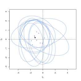
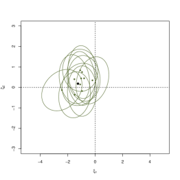
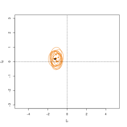
Figure 1: $95\%$ contours of predictive distributions $\bm{\xi}_{iK}|\mathbf{X}_{i},\mathbf{T}_{i}$ for a given subject and $K=2$, where we simulate $10$ possible time measurements for different number of observations $n_{i}$ in the transition from sparse to dense: Sparse $n_{i}=2$ (blue, left panel), medium sparse $n_{i}=10$ (green, middle panel) and dense $n_{i}=50$ (orange, right panel). The coloured dots correspond to the centers of the predictive distributions while the black dot shows the true latent FPCs.

The following theoretical framework is a direct consequence of the theory of square integrable Gaussian processes. For the separable real Hilbert space $\mathcal{H}=L^{2}(\mathcal{T})$ with inner product $\langle\ ,\ \rangle:=\langle\ ,\ \rangle_{L^{2}(\mathcal{T})}$, a probability measure $\nu$ defined over the Borel sets $\mathcal{B}(\mathcal{H})$ is Gaussian if for any $h\in\mathcal{H}^{*}$, where $\mathcal{H}^{*}$ denotes the dual space consisting of continuous and linear functionals on $\mathcal{H}$, $\mu\circ h$ is a Gaussian measure on $\mathbb{R}$ (Gelbrich, 1990). Such measures $\nu$ are characterized by their mean $m_{\nu}\in\mathcal{H}$ and covariance operator $\Xi_{\nu}:\mathcal{H}\to\mathcal{H}$ (Kuo, 1975), defined through

$$\langle m_{\nu},a\rangle =\int_{\mathcal{H}}\langle x,a\rangle\nu(dx),\quad a\in\mathcal{H},$$

$$\langle\Xi_{\nu}(a),b\rangle =\int_{\mathcal{H}}\langle x-m_{\nu},a\rangle\langle x-m_{\nu},b\rangle\nu(dx),\quad a,b\in\mathcal{H}.$$

Denote the Gaussian measure $\nu$ by $\mathbb{G}(m_{\nu},\Xi_{\nu})$. The $K$-truncated predictive distribution of the centered process $X_{i}^{c}(\cdot)$ given $(\mathbf{X}_{i},\mathbf{T}_{i})$ is defined as

$$\mathcal{G}_{iK}=(\text{The conditional distribution of }\bm{\xi}_{iK}^{T}\bm{\Phi}_{K}\mid\mathbf{X}_{i},\mathbf{T}_{i})=\mathbb{G}(\tilde{\mu}_{iK},\Xi_{iK}),$$

where $\tilde{\mu}_{iK}={\tilde{\bm{\xi}}_{iK}}^{T}\bm{\Phi}_{K}$, $\bm{\Phi}_{K}=(\phi_{1},\dots,\phi_{K})^{T}$ are the first $K$ eigenfunctions, and $\Xi_{iK}:L^{2}(\mathcal{T})\rightarrow L^{2}(\mathcal{T})$ is the integral operator associated with the covariance function $\Gamma_{iK}(s,t)\coloneqq\sum_{1\leq j,l\leq K}[\bm{\Sigma}_{iK}]_{jl}\phi_{j}(s)\phi_{l}(t)$, with $[\mathbf{A}]_{ij}$ denoting the $(i,j)$th entry of a matrix $\mathbf{A}$. This object is the functional (and finite-dimensional) counterpart of the $K$-truncated predictive distribution in (4) as it involves the first $K$ eigenfunctions $\bm{\Phi}_{K}$. We thus refer to $\mathcal{G}_{iK}$ as the $K$-truncated predictive distribution of the $i$th subject’s (unobserved) trajectory. The $K$-truncated predictive distribution $\mathcal{G}_{iK}$ is an approximation of the true infinite-dimensional predictive distribution,

$$\mathcal{G}_{i}=(\text{The conditional distribution of }(X-\mu)\mid\mathbf{X}_{i},\mathbf{T}_{i})=G(\tilde{\mu}_{i},\Xi_{i}),$$ (5)

where $\tilde{\mu}_{i}=\Gamma(\cdot,\mathbf{T}_{i})\bm{\Sigma}_{i}^{-1}(\mathbf{X}_{i}-\bm{\mu}_{i})$, $t\in\mathcal{T}$ and $\Xi_{i}$ is the integral operator associated with the covariance function $\Gamma_{i}(s,t)=\Gamma(s,t)-\Gamma(s,\mathbf{T}_{i})\bm{\Sigma}_{i}^{-1}\Gamma(\mathbf{T}_{i},t)$, $s,t\in\mathcal{T}$, under the convention that $\Gamma(s,\mathbf{T}_{i})$ and $\Gamma(\mathbf{T}_{i},t)$ are row and column vectors containing the evaluations of $\Gamma$, respectively. Next we study the approximation to the true latent trajectory as the truncation point $K$ increases in the transition from sparse to dense sampling.

The estimated versions to each of the previous objects are obtained by replacing population quantities by their estimates, leading to the following estimate for the $K$-truncated (functional) predictive distribution $\mathcal{G}_{iK}$,

$$\hat{\mathcal{G}}_{iK}=\mathbb{G}(\hat{\mu}_{iK},\hat{\Xi}_{iK}).$$

Here $\hat{\mu}_{iK}=\hat{\bm{\xi}}_{iK}^{T}\hat{\bm{\Phi}}_{K}$, and $\hat{\Xi}_{iK}$ is the integral operator associated with the covariance function $\hat{\Gamma}_{iK}(s,t)\coloneqq\sum_{1\leq j,l\leq K}[\hat{\bm{\Sigma}}_{iK}]_{jl}\hat{\phi}_{j}(s)\hat{\phi}_{l}(t)$. The infinite-dimensional version is

$$\hat{\mathcal{G}}_{i}=\mathbb{G}(\hat{\mu}_{i},\hat{\Xi}_{i}),$$ (6)

where $\hat{\mu}_{i}(t)=\hat{\Gamma}(t,\mathbf{T}_{i})\hat{\bm{\Sigma}}_{i}^{-1}(\mathbf{X}_{i}-\hat{\bm{\mu}}_{i})$, $t\in\mathcal{T}$ and $\hat{\Xi}_{i}$ is the integral operator associated with the covariance function $\hat{\Gamma}_{i}(s,t)\coloneqq\hat{\Gamma}(s,t)-\hat{\Gamma}(s,\mathbf{T}_{i})\hat{\bm{\Sigma}}_{i}^{-1}\hat{\Gamma}(\mathbf{T}_{i},t)$, $s,t\in\mathcal{T}$. In order to measure the discrepancy between estimated and true $K$-truncated (functional) predictive distributions, we require a suitable metric for probability measures with support in the Hilbert space $L^{2}$. For this purpose, we adopt the $2$-Wasserstein distance $\mathcal{W}_{2}$ due to its straightforward interpretation inherited from its connection to the optimal transport problem (Villani, 2003), and since it admits a simple form for Gaussian processes on a Hilbert space (Gelbrich, 1990) as well as for the distance between a Gaussian process and an atomic point mass, where the squared $\mathcal{W}_{2}$ distance is given by the mean of the squared $L^{2}$ distance between the Gaussian and the atomic element in the Hilbert space, which makes the $2$-Wasserstein distance a natural choice in our framework. For two measures $\nu$ and $\tau$, the $2$-Wasserstein metric is defined as

$$\mathcal{W}_{2}(\nu,\tau)=\left\{\inf_{A\sim\nu,B\sim\tau}E(\lVert A-B\rVert^{2})\right\}^{\frac{1}{{2}}},$$

where the norm $\lVert\cdot\rVert$ is either the Euclidean norm for measures supported on $\mathbb{R}^{d}$, $d\geq 1$, or $L^{2}$-norm for measures on the $L^{2}$ space, and the infimum is taken over all pairs of random variables $A$ and $B$ with marginal distribution $\nu$ and $\tau$, respectively (Villani, 2003). The $2$-Wasserstein distance between two Gaussian measures $\mathbb{G}(m_{\mu_{1}},\Xi_{\mu_{1}})$ and $\mathbb{G}(m_{\mu_{2}},\Xi_{\mu_{2}})$ over the infinite-dimensional Hilbert space $L^{2}(\mathcal{T})$ has a particularly simple form (Gelbrich, 1990),

$$\mathcal{W}_{2}^{2}(\mathbb{G}(m_{\mu_{1}},\Xi_{\mu_{1}}),\mathbb{G}(m_{\mu_{2}},\Xi_{\mu_{2}}))=\lVert m_{\mu_{1}}-m_{\mu_{2}}\rVert_{L^{2}}^{2}+\,\text{tr}(\Xi_{\mu_{1}}+\Xi_{\mu_{2}}-2(\Xi_{\mu_{1}}^{\frac{1}{2}}\Xi_{\mu_{2}}\Xi_{\mu_{1}}^{\frac{1}{2}})^{\frac{1}{2}}),$$

where for a positive, self-adjoint and compact operator $R:L^{2}(\mathcal{T})\rightarrow L^{2}(\mathcal{T})$, the square root operator $R^{\frac{1}{2}}$ is defined through its spectral decomposition (Hsing and Eubank, 2015). We then employ the $L^{2}$-Wasserstein distance on the space of $K$-truncated predictive distributions $\mathcal{G}_{iK}$, defined conditionally on both the measurements $\mathbf{X}_{i}$ and time observations $\mathbf{T}_{i}$. For the shrinkage in the $2$-Wasserstein metric of the $K$-truncated (functional) predictive distribution $\mathcal{G}_{iK}$ towards an atomic point mass measure $\mathcal{A}_{X_{i}^{c}}$ located at the unobserved latent centered process $X_{i}^{c}$ when the number of observations $n_{i}=m$ diverges and the truncation point $K=K(m)$ suitably grows with $m$, we obtain the following theorem.

Theorem 2.

Suppose that (S1)–(S4) and (B1) hold. Consider a given subject $i\in\{1,\dots,n\}$ which is densely observed $n_{i}=m\rightarrow\infty$. If $K=K(m)\rightarrow\infty$ is chosen such that $\sum_{k=1}^{K}\lambda_{k}^{-1}\asymp m^{1-\delta}$ for some $\delta\in(1/2,1)$, then as $m\rightarrow\infty$,

$$\mathcal{W}_{2}^{2}(\mathcal{G}_{iK},\mathcal{A}_{X_{i}^{c}}) =O_{p}\left(m^{-(2\delta-1)}+\sum_{k=K(m)+1}^{\infty}\lambda_{k}\right).$$ (7)

The expectation in the $2$-Wasserstein distance is taken here conditionally on the data for the $i$th subject $(\mathbf{X}_{i},\mathbf{T}_{i})$ and the unobserved latent trajectory $X_{i}^{c}$ so that the point mass $\mathcal{A}_{X_{i}^{c}}$ is well defined. Shrinkage of the $K$-truncated (functional) predictive distribution towards the latent centered process is inherently tied to the underlying eigenvalue decay. To illustrate the rate of convergence in (7), we consider examples of polynomial and exponential eigenvalue decay,

1. $\lambda_{k}=k^{-\alpha_{0}}$ for a constant $\alpha_{0}>1$ and all $k\geq 1$,

1. $\lambda_{k}=\,\text{exp}(-\alpha_{1}k)$ for a constant $\alpha_{1}>0$ and all $k\geq 1$.

Under polynomial decay rates (D1), it follows that $\sum_{k=1}^{K}\lambda_{k}^{-1}\asymp K^{1+\alpha_{0}}$ and also $\sum_{k=K+1}^{\infty}\lambda_{k}\asymp K^{1-\alpha_{0}}$, so the condition in Theorem 2 implies that $K\asymp m^{(1-\delta)/(1+\alpha_{0})}$ and the optimal rate in (7) is given by $m^{(1-\alpha_{0})/(1+3\alpha_{0})}$. This is achieved by choosing $\delta=2\alpha_{0}/(1+3\alpha_{0})$ and $K\asymp m^{1/(1+3\alpha_{0})}$. Faster eigenvalue decay rates for larger $\alpha_{0}$, are related to slower growth rates for $K=K(m)$ while $\delta$ approaches $2/3$. In this case the optimal rate approaches $m^{-1/3}$, which is slower than $m^{-1/2}$. The latter rate can be achieved for a finite-dimensional process, namely when $\lambda_{k}=0$ for all $k\geq k_{0}$ and some $k_{0}>0$. Under exponential eigenvalue decay rates (D2), the optimal rate in Theorem 2 is $m^{-1/3}$, which is obtained by selecting $\delta=2/3$ and $K\asymp\log(m^{1/3})$.

The previous result utilizes the population level $K$-truncated (functional) predictive distribution $\mathcal{G}_{iK}$, which depends upon unknown quantities that must be estimated in practice, introducing additional errors that need to be taken into account. The following result establishes consistency of the estimated $K$-truncated (functional) predictive distribution counterpart $\hat{\mathcal{G}}_{K}^{*}$ for a new independent subject as described in Section 2. For simplicity, let $\gamma_{K}(p,q)=\sum_{k=1}^{K}\lambda_{k}^{-p}\delta_{k}^{-q}$, where $p,q$ are non-negative integers and $\delta_{k}$ are eigengaps.

Theorem 3.

Suppose that assumptions (S2), (S4), (B1) and (A1)–(A8) in the Appendix are satisfied. Consider either a sparse design setting when $n_{i}\leq N_{0}<\infty$ or a dense design when $n_{i}=m\to\infty$, $i=1,\dots,n$. Set $a_{n}=a_{n1}$ and $b_{n}=b_{n1}$ for the sparse case, and $a_{n}=a_{n2}$ and $b_{n}=b_{n2}$ for the dense case. For a new independent subject $i^{*}$, suppose that $m^{*}=m^{*}(n)\to\infty$ is such that $m^{*}(a_{n}+b_{n})=o(1)$ as $n\rightarrow\infty$. If $K=K(m^{*})$ satisfies $(a_{n}+b_{n})\gamma_{K}(1/2,1)=o(1)$, $m^{*}(a_{n}+b_{n})^{2}\gamma_{K}(2,2)=o(1)$, $m^{*2}(a_{n}+b_{n})^{2}\gamma_{K}(2,0)=o(1)$, $m^{*4}(a_{n}+b_{n})^{4}\gamma_{K}(2,2)=o(1)$, $(a_{n}+b_{n})\gamma_{K}(2,1)=o(1)$ as $n\rightarrow\infty$, and $\sum_{k=1}^{K}\lambda_{k}^{-1}\asymp m^{*(1-\delta)}$ for some $\delta\in(1/2,1)$, then

$$\mathcal{W}_{2}^{2}(\hat{\mathcal{G}}_{K}^{*},\mathcal{A}_{X^{*c}}) =o_{p}(1).$$

For further details on the rates of convergence we refer to Section S.0.2 in the Supplement.

4 Predictive Distributions in the Functional Linear Model

Suppose one has an infinite-dimensional Gaussian predictor process $X(t)$, $t\in\mathcal{T}$, with Karhunen–Loève decomposition $X(t)=\mu(t)+\sum_{j=1}^{\infty}\xi_{j}\phi_{j}(t)$, and a Euclidean response $Y\in\mathbb{R}$, which are related through the FLM (1). Writing $\beta(t)=\sum_{j=1}^{\infty}\beta_{j}\phi_{j}(t)$, where $\beta_{j}=\int_{\mathcal{T}}\beta(t)\phi_{j}(t)$, $j=1,2,\dots$, (1) may be equivalently formulated as

$$E(Y|X^{c})=\beta_{0}+\sum_{j=1}^{\infty}\xi_{j}\beta_{j}=:\eta,$$ (8)

where $\beta_{0}=E(Y)$ is the intercept and $\eta$ is the linear predictor with responses $Y=\beta_{0}+\sum_{j=1}^{\infty}\xi_{j}\beta_{j}+\epsilon_{Y}$, where $\epsilon_{Y}\sim N(0,\sigma_{Y}^{2})$ is independent of all other random quantities.

Predicting the scalar response $Y$ (Hall and Horowitz, 2007) based on a sparsely observed predictor process $X$ is of great interest and has remained a challenging and unresolved issue as the FPCs of the predictor trajectory $X$ cannot be recovered consistently. Even knowledge of the true $\beta$ does not make it possible to consistently estimate the part of $Y$ that one expects to be consistently predictable, which is $\eta=E(Y|X^{c})=\int_{\mathcal{T}}\beta(s)X^{c}(s)ds$ in the FLM (1), notwithstanding the substantial literature on the consistency of estimates of the slope function $\beta$ in the case of fully observed (Cai and Hall, 2006) or sparsely sampled (Yao et al., 2005b) functional predictors.

Given this state of affairs, alternative approaches are needed. We propose to focus on predictive distributions of the linear predictor $\eta$, moving the target from constructing a point prediction to that of obtaining a predictive distribution for the response given the data available for the subject. We do not aim at the distribution for the observed response $Y$ as it also contains the additional error $\epsilon_{Y}$ that is independent of all other random quantities and thus is inherently unpredictable. To construct the distribution for the predictable part of the response $Y$, we consider $\eta_{K}=\beta_{0}+\bm{\beta}_{K}^{T}\bm{\xi}_{K}$, the truncated real-valued predictor employing the first $K$ principal components, where $K$ can be chosen by the FVE criterion and $\bm{\beta}_{K}=(\beta_{1},\dots,\beta_{K})^{T}$ are the (truncated) slope coefficients. Thus $\eta=\eta_{K}+\mathcal{R}_{K}$, where $\mathcal{R}_{K}=\sum_{j\geq K+1}\xi_{j}\beta_{j}$ corresponds to the linear predictor part that remains unexplained by $\eta_{K}$, but decreases asymptotically as $E(\mathcal{R}_{K})=0$ and $\,\text{Var}(\mathcal{R}_{K})=\sum_{j\geq K+1}\lambda_{j}\beta_{j}^{2}=o(1)$ as $K$ increases, where the latter rate can be specified under suitable assumptions (Hall and Horowitz, 2007).

Since $X$ is a Gaussian process, given $\bm{\beta}_{K}$, we can construct $\mathcal{P}_{iK}\overset{d}{=}N(\beta_{0}+\bm{\beta}_{K}^{T}\tilde{\bm{\xi}}_{iK},\bm{\beta}_{K}^{T}\bm{\Sigma}_{iK}\bm{\beta}_{K})$, which corresponds to a projection of the $K$-truncated predictive distribution of the FPC scores as derived above. According to Theorems 1 and 2, these predictive distributions collapse into a point mass located at the true but unobserved (truncated) predictable part $\eta_{iK}$ of the response $Y_{i}$ so that one can recover the predictable component up to the truncation point in the transition from sparse to dense sampling. To quantify the performance of the predictive distribution $\mathcal{P}_{iK}$ in the sparse case, we employ the 2-Wasserstein distance between two probability measures $\nu_{1},\nu_{2}$ on $\mathbb{R}$, which admits a simple form given by

$$\mathcal{W}_{2}^{2}(\nu_{1},\nu_{2}) =\int_{0}^{1}(Q_{1}(p)-Q_{2}(p))^{2}dp,$$ (9)

where $Q_{j}(p)=\inf\{s\in\mathbb{R}\colon F_{j}(s)\geq p\}$, $p\in(0,1)$, is the (generalized) quantile function corresponding to $\nu_{j}$, $j=1,2$ (Villani, 2003). As a measure of discrepancy of this predictive distribution we utilize the average Wasserstein distance between $\mathcal{P}_{iK}$ and the atomic measure $\mathcal{A}_{Y_{i}}$ located at $Y_{i}$. Formally,

$$\mathcal{D}_{nK}:=n^{-1}\sum_{i=1}^{n}\mathcal{W}_{2}^{2}(\mathcal{A}_{Y_{i}},\mathcal{P}_{iK}) =n^{-1}\sum_{i=1}^{n}(Y_{i}-\tilde{\eta}_{iK})^{2}+n^{-1}\sum_{i=1}^{n}\bm{\beta}_{K}^{T}\bm{\Sigma}_{iK}\bm{\beta}_{K},$$ (10)

where $\tilde{\eta}_{iK}=E(\eta_{iK}|\mathbf{X}_{i})=\beta_{0}+\bm{\beta}_{K}^{T}\tilde{\bm{\xi}}_{iK}$ is the best prediction of the (truncated) linear predictor, or equivalently the center of $\mathcal{P}_{iK}$. Note that (10) follows from (9) and similar ideas as in Amari and Matsuda (2021) when computing the Wasserstein distance between the predictive distribution and an atomic measure.

If the number of observations $n_{i}=m_{0}<N_{0}$ is common across subjects, so that the $\bm{\Sigma}_{iK}$ form an i.i.d. sequence of random positive definite matrices, the proof of Theorem 5 shows that $\mathcal{D}_{nK}$ converges to the population-level Wasserstein discrepancy

$$\mathcal{D}_{K}=2\bm{\beta}_{K}^{T}E(\bm{\Sigma}_{1K})\bm{\beta}_{K}+\sigma_{Y}^{2}+\sum_{k\geq K+1}\lambda_{k}\beta_{k}^{2}-2\bm{\beta}_{K}^{T}E\Big{[}\bm{\Lambda}_{K}\bm{\Phi}_{1K}^{T}\bm{\Sigma}_{1}^{-1}\sum_{k\geq K+1}\phi_{k}(\mathbf{T}_{1})\lambda_{k}\beta_{k}\Big{]}.$$ (11)

The first term in (11) reflects both the number of observations and the time locations, where increased values of $m_{0}$ are related to shrinkage of $\bm{\beta}_{K}^{T}E(\bm{\Sigma}_{1K})\bm{\beta}_{K}$ and thus lower discrepancy values, i.e. increased predictability. Similarly, increased predictor and response noise levels $\sigma^{2}$ and $\sigma_{Y}^{2}$ are associated with worse predictability. The last two terms come from the unexplained linear predictor part $\mathcal{R}_{K}$ and can be shrunk by increasing $K=K(n)$.

Consider an example with eigenbasis $\phi_{k}(t)=\sin(k\pi t)/\sqrt{2}$, $t\in\mathcal{T}$. If the Fourier coefficients $\beta_{k}$ and eigenvalues $\lambda_{k}$ exhibit polynomial decay $\lvert\beta_{k}\rvert=O(k^{-\alpha_{1}})$ and $\lambda_{k}=O(k^{-\alpha_{2}})$, $\alpha_{1},\alpha_{2}>1$, then by the Cauchy–Schwarz inequality we have $\sum_{k\geq K+1}\lambda_{k}\beta_{k}^{2}=O(K^{1-2\alpha_{1}-\alpha_{2}})$ and similarly $\bm{\beta}_{K}^{T}E[\bm{\Lambda}_{K}\bm{\Phi}_{1K}^{T}\bm{\Sigma}_{1}^{-1}\sum_{k\geq K+1}\phi_{k}(\mathbf{T}_{1})\lambda_{k}\beta_{k}]=O(K^{1-\alpha_{1}-\alpha_{2}})$ with $K^{1-\alpha_{1}-\alpha_{2}}\leq K^{-1}$, where we use that $\lVert\bm{\beta}_{K}\rVert_{2}\leq\lVert\beta\rVert_{L^{2}}$ and the uniform bound on the remaining quantities (see for example the proof of Lemma S12). In practice, the predictive distributions $\mathcal{P}_{iK}$ and therefore also the $\mathcal{D}_{nK}$ are unknown as they depend on unknown population quantities. We introduce $\hat{\mathcal{P}}_{iK}$ and $\hat{\mathcal{D}}_{nK}$, obtained by replacing population quantities by their estimated counterparts, where intercept $\beta_{0}$ and slope coefficients $\bm{\beta}_{K}$ are replaced by the below estimates.

Let $C(t)=\,\text{Cov}(X(t),Y)=\sum_{k=1}^{\infty}E(Y\xi_{k})\phi_{k}(t)$ be the cross-covariance function between the process $X$ and response $Y$ and $\sigma_{k}=\int_{\mathcal{T}}C(t)\phi_{k}(t)dt=E(Y\xi_{k})$, $k=1,2,\dots$. We estimate $C(t)$ using a local linear smoother on the raw covariances $C_{i}(T_{ij})=(\tilde{X}_{ij}-\hat{\mu}(T_{ij}))Y_{i}$ (Yao et al., 2005b), leading to an estimate $\hat{C}(t)$ depending on a bandwidth $h$; see Section S.0.1 in the Supplement for details. Since $\sigma_{k}=\lambda_{k}\beta_{k}$, under the following common regularity condition,

1. $\lVert\beta\rVert_{L^{2}}^{2}=\sum_{m=1}^{\infty}\sigma_{m}^{2}/\lambda_{m}^{2}<\infty$,

it holds that $\beta(t)=\sum_{m=1}^{\infty}\sigma_{m}\phi_{m}(t)/\lambda_{m}$, $t\in\mathcal{T}$. This motivates to estimate $\beta$ by

$$\hat{\beta}_{M}(t)=\sum_{m=1}^{M}\frac{\hat{\sigma}_{m}}{\hat{\lambda}_{m}}\hat{\phi}_{m}(t),\quad t\in\mathcal{T},$$

where $\hat{\sigma}_{k}=\int_{\mathcal{T}}\hat{C}(t)\hat{\phi}_{k}(t)dt$ is an estimate of $\sigma_{k}$ and $M=M(n)$ is a positive integer sequence that diverges as $n\rightarrow\infty$. The intercept $\beta_{0}=E(Y)$ is estimated by $\hat{\beta}_{0}=n^{-1}\sum_{i=1}^{n}Y_{i}$. Convergence of $\hat{\beta}_{M}$ towards $\beta$ is tied to the eigengaps of $X$ (Cai and Hall, 2006; Müller and Yao, 2010).

With estimates $\hat{\beta}_{M}$ of $\beta$ in hand, we can readily construct the predictive distributions $\hat{\mathcal{P}}_{iK}$. For the following and in the sparse case, we assume for simplicity that the optimal asymptotic tuning parameters are used for estimating the mean, covariance and cross-covariance, $h_{\mu}\asymp(\log n/n)^{1/5}$, $h_{G}\asymp(\log n/n)^{1/6}$ (Dai et al., 2018) and $h\asymp n^{-1/3}$ in the sparse design situation; in particular, this implies $c_{n}:=\max(a_{n},b_{n})\asymp(\log n/n)^{1/3}$. Defining sequences $\upsilon_{M}=\sum_{m=1}^{M}\delta_{m}^{-1}$, $\tau_{M}=\sum_{m=1}^{M}\lambda_{m}^{-1}$ and a remainder term $\Theta_{M}=\lVert\sum_{m\geq M+1}(\sigma_{m}/\lambda_{m})\phi_{m}\rVert_{L^{2}}$, where $\delta_{m}$ are the eigengaps, we note that $M=M(n)$ should not grow too fast with sample size $n$, which we formalize in the following assumption,

1. The integer sequence $M=M(n)\to\infty$ as $n\to\infty$ is such that $\sum_{m=1}^{M}\lambda_{m}^{-1/2}\delta_{m}^{-1}=O(c_{n}^{\rho-1})$ for some $\rho\in(1/3,1)$,

with an additional regularity assumption to obtain uniform convergence,

1. There exist a scalar $\kappa_{0}>0$ such that $\lambda_{\min}(\bm{\Sigma}_{iK})\geq\kappa_{0}$ almost surely, for all $i\geq 1$.

(C1) is a mild assumption, as $\bm{\Sigma}_{iK}$ corresponds to the conditional variance of $\bm{\xi}_{iK}-\tilde{\bm{\xi}}_{iK}$ given $\mathbf{T}_{i}$, which is positive definite and cannot shrink to zero in the sparse case due to the constraint on the number of observations per subject $n_{i}\leq N_{0}<\infty$.

Our next result demonstrates that $\hat{\mathcal{P}}_{iK}$ is consistent for $\mathcal{P}_{iK}$ in the $2$-Wasserstein metric, the Kolmogorov metric and in the $L^{2}$ metric between the corresponding predictive densities. Let $F_{iK}$ denote the cumulative distribution function corresponding to $\mathcal{P}_{iK}\overset{d}{=}N(\beta_{0}+\bm{\beta}_{K}^{T}\tilde{\bm{\xi}}_{iK},\bm{\beta}_{K}^{T}\bm{\Sigma}_{iK}\bm{\beta}_{K})$ and $\hat{F}_{iK}$ the corresponding cdf obtained by replacing $\tilde{\bm{\xi}}_{iK}$ and $\bm{\Sigma}_{iK}$ by $\hat{\bm{\xi}}_{iK}$ and $\hat{\bm{\Sigma}}_{iK}$, respectively, and $\beta_{0}$ and $\bm{\beta}_{K}$ by the above estimates. Denote the estimated and true predictive densities by $\hat{f}_{i}(t)=d\hat{F}_{i}(t)/dt$ and $f_{i}(t)=dF_{i}(t)/dt$. For a function $g\colon\mathcal{T}\to\mathbb{R}$, let $\lVert g\rVert_{L^{2}(\mathbb{R})}=(\int_{\mathbb{R}}g^{2}(s)ds)^{1/2}$ denote its $L^{2}$ norm over $\mathbb{R}$.

1. Let $c_{n}=\max(a_{n},b_{n})\rightarrow 0$ as $n\rightarrow\infty$, where $a_{n}$ and $b_{n}$ are defined in (3).

Theorem 4.

Suppose that (S4), (B1)–(B4), (A1)–(A8) in the Appendix hold, and consider a sparse design with $n_{i}\leq N_{0}<\infty$. For a fixed $K\geq 1$, setting $a_{n}=a_{n1}$ and $b_{n}=b_{n1}$,

$$\mathcal{W}_{2}(\hat{\mathcal{P}}_{iK},\mathcal{P}_{iK}) =O_{p}(\alpha_{n}),$$ (12)

$$\sup_{t\in\mathbb{R}}\ \lvert\hat{F}_{iK}(t)-F_{iK}(t)\rvert =O_{p}(\alpha_{n}),$$ (13)

$$\lVert\hat{f}_{iK}-f_{iK}\rVert_{L^{2}(\mathbb{R})} =O_{p}(\alpha_{n}),$$ (14)

as $n\rightarrow\infty$, where $\alpha_{n}=c_{n}\upsilon_{M}+c_{n}^{\rho}\tau_{M}^{1/2}+\Theta_{M}$ and the $O_{p}(\alpha_{n})$ terms are uniform in $i$.

Under the conditions of Theorem 4, $\alpha_{n}\rightarrow 0$ is a consequence of $\tau_{M}\leq\upsilon_{M}=O(c_{n}^{\rho-1})$, which implies $\alpha_{n}\leq O(c_{n}^{(3\rho-1)/2}+\Theta_{M})$. There is a trade-off between how fast $M$ can grow and the rate of convergence for the estimates of the population quantities, where a larger $M$ entails a lower remainder term $\Theta_{M}$ but affects the rate at which $\beta$ is recovered through $\hat{\beta}_{M}$, which involves $M$ components, and vice versa. Since the former term is connected to the decay of the covariance terms $\sigma_{m}/\lambda_{m}$, the optimal growth rate of $M(n)$ is inherently tied to the decay rate of $\sigma_{m}$, $\lambda_{m}$ and the eigengaps $\delta_{m}$. For additional discussion, see Section S.0.2 in the supplement.

Regarding the Wasserstein discrepancy $\mathcal{D}_{nK}$, we show next that the proposed predictability measure and the response measurement error variance $\sigma_{Y}^{2}$ can be consistently estimated in the sparse case. We consider the special case when the number of observations $n_{i}=m_{0}<N_{0}$ is common across subjects, and show that the estimated Wasserstein discrepancy measure $\hat{\mathcal{D}}_{nK}$ converges to the population target $\mathcal{D}_{K}$, which is inherently related to the predictability of the response by the $K$-truncated predictive distribution.

Theorem 5.

Suppose that (S4), (B1)–(B4), (C1), (A1)–(A8) in the Appendix hold and consider a sparse design with $n_{i}=m_{0}\leq N_{0}<\infty$, setting $a_{n}=a_{n1}$ and $b_{n}=b_{n1}$. For $K\geq 1$,

$$\hat{\mathcal{D}}_{nK} =\mathcal{D}_{K}+O_{p}(\alpha_{n}),\quad\alpha_{n}=c_{n}\upsilon_{M}+c_{n}^{\rho}\tau_{M}^{1/2}+\Theta_{M},$$ (15)

and furthermore

$$n^{-1}\sum_{i=1}^{n}(Y_{i}-\bar{Y}_{n})^{2}-\sum_{m=1}^{M}\hat{\lambda}_{j}\hat{\beta}_{j}^{2} =\sigma_{Y}^{2}+O_{p}(\alpha_{n})+\sum_{m\geq M+1}\lambda_{m}\beta_{m}^{2},\quad\text{with}\quad\bar{Y}_{n}=n^{-1}\sum_{i=1}^{n}Y_{i}.$$ (16)

We next consider the behavior of the estimated predictive distributions under the transition from sparse to dense sampling for a new independent subject $i^{*}$ as in Section 2.

Theorem 6.

Suppose that assumptions (S2), (S4), (B1)–(B4) and (A1)–(A8) in the Appendix are satisfied. Consider either a sparse design setting when $n_{i}\leq N_{0}<\infty$ or a dense design when $n_{i}=m\to\infty$, $i=1,\dots,n$. Set $a_{n}=a_{n1}$ and $b_{n}=b_{n1}$ for the sparse case, and $a_{n}=a_{n2}$ and $b_{n}=b_{n2}$ for the dense case. Let $K>0$ be fixed and take $h=n^{-1/3}$. For a new independent subject $i^{*}$, suppose that $m^{*}=m^{*}(n)\to\infty$ is such that $m^{*}(a_{n}+b_{n})=o(1)$ as $n\rightarrow\infty$. Then

$$\mathcal{W}_{2}^{2}(\mathcal{P}_{K}^{*},\mathcal{A}_{\beta_{0}+\bm{\beta}_{K}^{T}\bm{\xi}_{K}^{*}}) =O_{p}(m^{*-1}),$$

and

$$\mathcal{W}_{2}^{2}(\hat{\mathcal{P}}_{K}^{*},\mathcal{A}_{\beta_{0}+\bm{\beta}_{K}^{T}\bm{\xi}_{K}^{*}}) =O_{p}\left(m^{*2}(a_{n}+b_{n})^{2}+m^{*-1}+a_{n}+b_{n}+r_{n}^{*2}\right),$$

where $r_{n}^{*}=c_{n}\upsilon_{M}+c_{n}^{\rho}\tau_{M}^{1/2}+\tau_{M}\Big{[}n^{-1/3}+a_{n}\Big{]}+\Theta_{M}$.

5 Simulations

We consider a finite-dimensional Gaussian process $X(t)$, $t\in\mathcal{T}=[0,10]$, using $K=4$ principal components, where the population quantities are given by $\phi_{1}(t)=-\cos(\pi t/10)/\sqrt{5}$, $\phi_{k}(t)=\sin((2k-3)\pi t/10)/\sqrt{5}$, $k=2,\dots,K$, $\mu(t)=t/2$, $\lambda_{k}=4/(1+k)^{2}$, $k=1,\dots,K$. For the functional linear model, the intercept and slope coefficients are given by $\beta_{0}=0.5$, $\beta_{1}=1$, $\beta_{2}=-1$, $\beta_{3}=0.5$ and $\beta_{4}=-0.5$. We investigate different noise levels in the predictor process $X$ and response $Y$ as well as different sparse settings, where we generate $n_{i}=m_{0}$ random time points for the $i$th subject, $i=1,\dots,n$. Here $m_{0}=2$ reflects a very sparse design, $m_{0}=8$ a medium sparse and $m_{0}=20$ a dense case. Then, given the number $n_{i}$, we select the time points at random and without replacement from an equispaced grid of $100$ points over $\mathcal{T}$. We perform $2,000$ simulations, where the methods were implemented in Julia, interfacing with R and the fdapace package (Gajardo et al., 2021).

Table 1 presents the results for the Wasserstein discrepancy $\hat{\mathcal{D}}_{nK}$ under different sparsity designs and noise levels in both the functional predictor and scalar response $Y$. The discrepancy $\hat{\mathcal{D}}_{nK}$ reflects the improvements in predictability for lower noise levels and under increasingly denser designs and increases monotonically in both $\sigma$ and $\sigma_{Y}$ and decreases monotonically as the design becomes denser when keeping the noise level $\sigma$ and $\sigma_{Y}$ fixed.

Table 1: Simulation results for the Wasserstein discrepancy $\hat{\mathcal{D}}_{nK}$, which measures the predictability of the response $Y_{i}$ by the predictive distribution $\mathcal{P}_{iK}$. The true regression parameters are $\beta_{0}=0.5$ and $\bm{\beta}_{K}=(1,-1,0.5,-0.5)^{T}$. Different predictor and response measurement error levels and sparsity levels are investigated, where very sparse corresponds to $n_{i}=2$ observations per subject, for medium sparse $n_{i}=8$ and for dense design $n_{i}=20$. The values in the table are the averages of $\hat{\mathcal{D}}_{nK}$ across 2000 simulations.

Measurement Error Noise level		Sparsity setting
Predictor	Response	Very Sparse		Medium Sparse		Dense
$\sigma$	$\sigma_{Y}$	$n=500$	$n=2000$	$n=500$	$n=2000$	$n=500$	$n=2000$
	0.5	3.008	2.645	1.492	1.477	0.863	0.853
0.5	1.0	3.863	3.421	2.255	2.237	1.612	1.606
1.0	0.5	3.639	3.449	2.540	2.418	1.729	1.715

As an additional measure of performance for $\mathcal{P}_{iK}$, we computed the estimated $2$-Wasserstein distance between the empirical distribution of $\hat{F}_{iK}(\beta_{0}+\int_{\mathcal{T}}\beta(s)(X_{i}(s)-\mu(s))ds)$, $i=1,\dots,n$, and a uniform distribution on $(0,1)$. This is of interest by observing that $F_{1K}(\eta_{1K}),\dots,F_{nK}(\eta_{nK})$ constitute an i.i.d. sample from a uniform random variable $U$ in $(0,1)$. A conditioning argument gives $P(F_{iK}(\eta_{iK})\leq p)=E(P(F_{iK}(\eta_{iK})\leq p|\mathbf{X}_{i}))=E(P(\eta_{iK}\leq F_{iK}^{-1}(p)|\mathbf{X}_{i}))=p$, $p\in(0,1)$. Thus, if we denote by $F_{K}(\eta_{K})$ a generic probability transformation of the linear response $\eta_{K}$ through the cdf corresponding to $\eta_{K}|\mathbf{X}$, then one should expect the random variable $F_{K}(\eta_{K})$ to be close to a uniform distribution over $(0,1)$, where we utilize the $2$-Wasserstein distance to measure the discrepancy between these distributions,

$$\mathcal{W}_{2}^{2}(F_{K}(\eta_{K}),U) =\int_{0}^{1}(Q_{K}(p)-p)^{2}dp,$$ (17)

where $Q_{K}$ is the quantile function of the random variable $F_{K}(\eta_{K})$. Since the quantities $F_{1K}(\eta_{1K}),\dots,F_{nK}(\eta_{nK})$ are i.i.d. and share the same distribution with $F_{K}(\eta_{K})$, we may estimate $Q_{K}$ by the empirical quantile of the $F_{iK}(\eta_{iK})$.

Defining $Z_{i}$ to be the $i$th order statistic of the $F_{jK}(\eta_{jK})$, $j=1,\dots,n$, a natural estimate $U_{\mathcal{W}}$ of $W_{2}^{2}(F_{K}(\eta_{K}),U)$ in (17) is given by (Amari and Matsuda, 2021)

$$U_{\mathcal{W}} =\sum_{i=1}^{n}\frac{z_{i}^{2}}{n}-z_{i}\left(\frac{i^{2}}{n^{2}}-\frac{(i-1)^{2}}{n^{2}}\right)+\frac{1}{3}\left(\frac{i^{3}}{n^{3}}-\frac{(i-1)^{3}}{n^{3}}\right),$$

and we define $\hat{U}_{\mathcal{W}}$ analogously after replacing population quantities by their estimated versions. Table 2 shows the simulations results, where one finds that as $n$ increases, the distance $\hat{U}_{\mathcal{W}}$ diminishes, which reflects better performance of the predictive distributions $\mathcal{P}_{iK}$. Higher noise levels have worse performance as it becomes harder to estimate population quantities with the same sample size. Similarly, denser designs have a lower average value of $\hat{U}_{\mathcal{W}}$ as expected.

Table 2: Simulation results for the Wasserstein measure against a uniform distribution $\hat{U}_{\mathcal{W}}$ defined through (17) for the same settings as in Table 1, displaying the averages of $\hat{U}_{\mathcal{W}}$ across simulations. Values in the table are scaled by a factor $1,000$.

Measuremet Error Noise level		Sparsity setting
Predictor	Response	Very Sparse		Medium Sparse		Dense
$\sigma$	$\sigma_{Y}$	$n=500$	$n=2000$	$n=500$	$n=2000$	$n=500$	$n=2000$
	0.5	1.74	0.62	0.85	0.46	0.76	0.37
0.5	1.0	2.18	0.75	1.22	0.58	1.25	0.52
1.0	0.5	2.95	1.54	1.05	0.44	0.82	0.45

6 Data Illustration

We showcase the concept of predictive distributions for longitudinal data in the context of functional linear regression models. We showcase this construction for the body mass index (BMI) and systolic blood pressure (SBP) data in the Baltimore Longitudinal Study of Aging (BLSA, Shock et al., 1984), where variables are measured sparsely over time for each subject. This dataset has been analyzed previously for a sparse FLM regression framework in Yao et al. (2005b), to which we refer for further details.

We consider a sample of male subjects such that their age in years falls in the interval $[50,80]$ and for which their SBP and BMI measurements are within the corresponding first and third quartiles across all subjects. For the estimation of population quantities, we employ the fdapace R package (Gajardo et al., 2021) and construct estimated predictive distributions as described in Section 4. For this, we regress SPB (in mm Hg) at the last age where it is measured as scalar response against the sparsely observed functional predictor (BMI in kg/$m^{2}$). We utilize the first $K=3$ FPC scores of the BMI trajectory, which are found to explain more than $98\%$ of the variation, and choose $M=K$ components and the cross-covariance bandwidth $h$ by leave-one-out cross-validation. Figure 2 shows the predictive distribution intervals constructed from the $5\%$ and $95\%$ quantiles of $\hat{\mathcal{P}}_{iK}$ for $5$ randomly selected subjects with at least $5$ measurements. The dots correspond to the individual response observations $Y_{i}$.

We remark that since the predictive distribution targets the (truncated) predictable part of the response $Y_{i}$, which is contaminated with unpredictable measurement error $\epsilon_{iY}$, it is not expected for $Y_{i}$ to fall within a confidence interval constructed from $\mathcal{P}_{iK}$ with the corresponding significance level. Instead, the predictive intervals target the true truncated predictable part $\eta_{iK}=\beta_{0}+\bm{\beta}_{K}^{T}\bm{\xi}_{iK}$ of the observed response $Y_{i}$, which is close to the linear predictor part $\eta_{i}=\beta_{0}+\sum_{k=1}^{\infty}\beta_{k}\xi_{ik}$ at least for a large enough truncation point $K$.

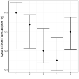
Figure 2: Predictive distribution intervals constructed from the $5\%$ and $95\%$ quantiles of $\hat{\mathcal{P}}_{iK}$ for $5$ randomly selected subjects with a median SBP between the first and third quartiles, and at least $5$ measurements. Here the regression features SBP at the last age with a measurement as response and the sparsely measured BMI trajectory as predictor for the BLSA dataset. The individual dots correspond to the observed SBP for the subject.

Assumptions

We assume the following regularity conditions (A1)–(A8), which are similar to those in Zhang and Wang (2016) and Dai et al. (2018), and are presented here for completeness. Recall that $w_{i}=\left(\sum_{j=1}^{n}n_{j}\right)^{-1}$ and $v_{i}=\left(\sum_{j=1}^{n}n_{j}(n_{j}-1)\right)^{-1}$.

1. $K(\cdot)$ is a symmetric probability density function on $[-1,1]$ and is Lipschitz continuous: There exists $0<L<\infty$ such that $|K(u)-K(v)|\leq L|u-v|$ for any $u,v\in[0,1]$.

2. $\{T_{ij}:i=1,\dots,n,\,j=1,\dots,n_{i}\}$ are i.i.d. copies of a random variable $T$ defined on $\mathcal{T}$, and $n_{i}$ are regarded as fixed. The density $f(\cdot)$ of $T$ is bounded below and above,

   $$0<m_{f}\leq\min_{t\in\mathcal{T}}f(t)\leq\max_{t\in\mathcal{T}}f(t)\leq M_{f}<\infty.$$

   Furthermore $f^{(2)}$, the second derivative of $f(\cdot)$, is bounded.

3. $X$, $\epsilon$, and $T$ are independent.

4. $\mu^{(2)}(t)$ and $\partial^{2}\Gamma(s,t)/\partial s^{p}\partial t^{2-p}$ exist and are bounded on $\mathcal{T}$ and $\mathcal{T}\times\mathcal{T}$, respectively, for $p=0,\dots,2$.

5. $h_{\mu}\rightarrow 0$, $\log(n)\sum_{i=1}^{n}n_{i}w_{i}^{2}/h_{\mu}\rightarrow 0$ and $\log(n)\sum_{i=1}^{n}n_{i}(n_{i}-1)w_{i}^{2}\rightarrow 0$ .

6. For some $\alpha>2$, $E(\sup_{t\in\mathcal{T}}|X(t)-\mu(t)|^{\alpha})<\infty$, $E(|\epsilon|^{\alpha})<\infty$, and

   $$n\left[\sum_{i=1}^{n}n_{i}w_{i}^{2}h_{\mu}+\sum_{i=1}^{n}n_{i}(n_{i}-1)w_{i}^{2}h_{\mu}^{2}\right]\left[\frac{\log(n)}{n}\right]^{2/\alpha-1}\rightarrow\infty.$$

7. $h_{G}\rightarrow 0$, $\log(n)\sum_{i=1}^{n}n_{i}(n_{i}-1)v_{i}^{2}/h_{G}^{2}\rightarrow 0$ and $\log(n)\sum_{i=1}^{n}n_{i}(n_{i}-1)(n_{i}-2)v_{i}^{2}/h_{G}\rightarrow 0$.

8. For some $\beta_{\gamma}>2$, $E(\sup_{t\in\mathcal{T}}|X(t)-\mu(t)|^{2\beta_{\gamma}})<\infty$, $E(|\epsilon|^{2\beta_{\gamma}})<\infty$, and

   $$n\bigg{[} \sum_{i=1}^{n}n_{i}(n_{i}-1)v_{i}^{2}h_{G}^{2}+\sum_{i=1}^{n}n_{i}(n_{i}-1)(n_{i}-2)v_{i}^{2}h_{G}^{3}$$

   $$+\sum_{i=1}^{n}n_{i}(n_{i}-1)(n_{i}-2)(n_{i}-3)v_{i}^{2}h_{G}^{4}\bigg{]}\left[\frac{\log(n)}{n}\right]^{2/\beta_{\gamma}-1}\rightarrow\infty.$$

We remark that assumption (A2) implies (S1) and assumption (A4) implies (S3).

Supplementary Material

For notational simplicity, for a function $g_{1}:\mathcal{T}\to\mathbb{R}$ and a vector $\bm{z}=(z_{1},\dots,z_{p})^{T}\in\mathbb{R}^{p}$, $p>0$, denote by $g_{1}(\bm{z})=(g_{1}(z_{1}),\dots,g_{1}(z_{p}))^{T}$ the application of $g_{1}$ to $\bm{z}$ entry-wise. Similarly, for a function $g_{2}:\mathcal{T}\times\mathcal{T}\to\mathbb{R}$ and a second vector $\bm{r}=(r_{1},\dots,r_{q})^{T}\in\mathbb{R}^{q}$, $q>0$, denote by $g_{2}(\bm{z},\bm{r}^{T})$ the $p\times q$ matrix, for which the $(l,k)$ element is given by $g_{2}(z_{l},r_{k})$, where $1\leq l\leq p$ and $1\leq k\leq q$. Also, for two scalar sequences $\theta_{n}$ and $\gamma_{n}$, denote by $\theta_{n}\lesssim\gamma_{n}$ if there exists a constant $c_{0}>0$ such that $\theta_{n}\leq c_{0}\gamma_{n}$ holds for large enough $n$.

S.0 Additional Details

S.0.1 Mean and Covariance Estimation

For the mean function estimate, set $\hat{\mu}(t)=\hat{\gamma}_{0}$, where

$$(\hat{\gamma}_{0},\hat{\gamma}_{1}) =\operatorname*{argmin}_{\gamma_{0},\gamma_{1}}\sum_{i=1}^{n}w_{i}\sum_{j=1}^{n_{i}}(X_{ij}-\gamma_{0}-\gamma_{1}(T_{ij}-t))^{2}K_{h_{\mu}}(T_{ij}-t),$$

where $w_{i}=(\sum_{j=1}^{n}n_{j})^{-1}$ are equal subject weights, $K$ is a kernel function corresponding to a density function with compact support $[-1,1]$ and $K_{h_{\mu}}(\cdot)=K(\cdot/h_{\mu})/h_{\mu}$. For the covariance surface estimate, denoting by $\hat{C}_{ijl}=(X_{ij}-\hat{\mu}(T_{ij}))(X_{il}-\hat{\mu}(T_{il}))$ the raw covariances (Yao et al., 2005a), set $\hat{\Gamma}(s,t)=\hat{\gamma}_{0}$, where

$$(\hat{\gamma}_{0},\hat{\gamma}_{1},\hat{\gamma}_{2})$$

$$=\operatorname*{argmin}_{\gamma_{0},\gamma_{1},\gamma_{2}}\sum_{i=1}^{n}v_{i}\sum_{1\leq j\neq l\leq n_{i}}(C_{ijl}-\gamma_{0}-\gamma_{1}(T_{ij}-s)-\gamma_{2}(T_{il}-t))^{2}K_{h_{G}}(T_{ij}-s)K_{h_{G}}(T_{il}-t),$$

where $v_{i}=(\sum_{j=1}^{n}n_{j}(n_{j}-1))^{-1}$ and $n_{i}\geq 2$ is assumed throughout for the covariance estimation step.

For the cross-covariance smoothing step, recalling the raw covariances $C_{i}(T_{ij})=(\tilde{X}_{ij}-\hat{\mu}(T_{ij}))Y_{i}$, then the local linear estimate of $C(t$ is given by $\hat{C}(t)=\hat{\beta}_{0}^{X}$, where

$$(\hat{\beta}_{0}^{X},\hat{\beta}_{1}^{X})=\operatorname*{argmin}_{\beta_{0}^{X},\beta_{1}^{X}\in\mathbb{R}}\ \sum_{i=1}^{n}\sum_{j=1}^{n_{i}}w_{i}K_{h}(T_{ij}-t)(C_{i}(T_{ij})-\beta_{0}^{X}-\beta_{1}^{X}(t-T_{ij}))^{2},$$ (S.18)

and $w_{i}=(\sum_{i=1}^{n}n_{i})^{-1}$.

S.0.2 More details on rates of convergence

Rates for Theorem 1. For two sequences $\theta_{n}$ and $\gamma_{n}$ denote by $\theta_{n}\asymp\gamma_{n}$ whenever $c_{1}\theta_{n}\leq\gamma_{n}\leq c_{2}\theta_{n}$ holds for some constants $c_{1},c_{2}>0$ as $n\rightarrow\infty$. For a dense design, if the number of individual observations $m=m(n)$ satisfies $m\asymp(n/\log n)^{q}$ for some $q\in[1/4,\infty)$, $h_{\mu}\asymp(\log n/n)^{1/4}$, $h_{G}\asymp(\log n/n)^{\rho}$ with $\rho\in(0,1/4)$, $\alpha$ defined in (A6) satisfies $\alpha>4$, $\beta_{\gamma}$ defined in (A8) is such that $\beta_{\gamma}>2/(1-4\rho)$, then $a_{n}+b_{n}\asymp(\log n/n)^{2\rho}$. A larger value of $\rho\in(0,1/4)$ along with the existence of a suitable $\beta_{\gamma}=\beta_{\gamma}(\rho)$ as before leads to a rate $a_{n}+b_{n}$ closer to $(\log n/n)^{1/2}$. Here the choice $0<\rho<1/4$, which entails the rate for the covariance smoothing bandwidth $h_{G}$, is required in order to satisfy condition (A8) or equivalently assumption (D2c) in Zhang and Wang (2016). If $m^{*}\asymp(a_{n}+b_{n})^{-\rho_{1}}$ for some $\rho_{1}\in(0,1)$, then the condition $m^{*}(a_{n}+b_{n})=o(1)$ is satisfied and the rate in Theorem 1 becomes $O_{p}((\log n/n)^{\rho_{1}\rho}+(\log n/n)^{1-\rho_{1}})$. Hence, larger values of $\rho\in(0,1/4)$ along with the optimal choice $\rho_{1}=2/3$ leads to an optimal rate arbitrarily close to $O_{p}((\log n/n)^{1/6})$.

Rates for Theorem 3. Under polynomial eigenvalue decay rates (D1) and taking $m^{*}=m^{*}(n)\asymp(a_{n}+b_{n})^{-q}$ for some $q\in(0,2/3)$, it follows from the proof of Theorem 3 that the optimal rate is given by $(a_{n}+b_{n})^{q(\alpha_{0}-1)/(3\alpha_{0}+1)}$, which is achieved by taking $\delta=2\alpha_{0}/(3\alpha_{0}+1)\in(1/2,1)$ and $K\asymp m^{*(1-\delta)/(1+\alpha_{0})}$. Thus, the optimal rate can be arbitrarily close to $(a_{n}+b_{n})^{2(\alpha_{0}-1)/(3(1+3\alpha_{0}))}$ by taking faster growth rates of $m^{*}$ with $q\uparrow 2/3$. Faster eigenvalue decay rate, i.e. larger values of $\alpha_{0}$, leads to a rate closer to $(a_{n}+b_{n})^{2/9}$. If the eigenvalues exhibit exponential decay (D2) and $m^{*}=m^{*}(n)\asymp(a_{n}+b_{n})^{-q}$, $q\in(0,1)$, the optimal rate is $(a_{n}+b_{n})^{2/9}$.

Rates for Theorem 4. We consider the special case where $X$ is a Brownian motion, for which the $\lambda_{m}$ and $\phi_{m}$ are known (Hsing and Eubank, 2015). Although Brownian motion does not satisfy the smoothness assumptions required, it still serves as a simple example to provide insight into how the convergence rate is related to the eigenvalue decay of the process. Lemma S16 in the Supplement shows that if $M=M(n)\asymp(\log n/n)^{(\rho-1)/15}$, then $M$ satisfies (B3) with $\sum_{m=1}^{M}\lambda_{m}^{-1/2}\delta_{m}^{-1}\asymp c_{n}^{\rho-1}$. Moreover, if the decay of $\sigma_{m}$ is such that $\sigma_{m}^{2}\leq Cm^{-(8+\delta)}$ for some constant $C>0$ and $\delta>0$, then (B2) is satisfied, the remainder $\Theta_{M}=O\left(M^{-(1+\delta/2)}\right)$ and the rate $\alpha_{n}$ satisfies the following conditions as stated in Lemma S16: If $\rho\leq(5+\delta)/(15+\delta)$, then $\alpha_{n}=O((\log n/n)^{(13\rho-3)/30})$ while if $\rho>(5+\delta)/(15+\delta)$ it holds that $\alpha_{n}=O((\log n/n)^{(1-\rho)(1+\delta/2)/15})$. The optimal rate is achieved when $\rho=(5+\delta)/(15+\delta)$ and leads to $\alpha_{n}=O((\log n/n)^{q})$, where $q=((2+\delta)/(15+\delta))/3$. A sufficiently large $\delta$ implies that $q$ is closer to $1/3$ so that the rate $\alpha_{n}$ approaches $c_{n}=(\log n/n)^{1/3}$, which is the rate at which population quantities such as the covariance function $\Gamma$ are uniformly recovered (see e.g. Theorem $5.2$ in Zhang and Wang (2016)).

S.1 Auxiliary Results and Proofs of Main Results in Section 3

In this section we provide auxiliary lemmas which will be used to derive the main results in section 3. For the next lemma, we say that a process $X$ is explained by its first $K$ principal components if $X(t)=\mu(t)+\sum_{k=1}^{K}\xi_{k}\phi_{k}(t)$ and thus it is of finite dimension $K$.

Lemma S1.

Suppose that the process $X$ is finite dimensional and explained by its first $K=2$ principal components. If $\phi_{1}$ and $\phi_{2}$ are bijective and differentiable in a finite partition of $\mathcal{T}$, then $\bm{\Sigma}_{iK}$ has a positive eigengap almost surely.

of Lemma S1.

Recalling that $\bm{\Sigma}_{iK}=\bm{\Lambda}_{K}-\bm{\Lambda}_{K}\bm{\Phi}_{iK}^{T}\bm{\Sigma}_{i}^{-1}\bm{\Phi}_{iK}\bm{\Lambda}_{K}$ and since $K=2$, it follows that the characteristic polynomial of $\bm{\Sigma}_{iK}$ is given by $p(\lambda)=\lambda^{2}-\,\text{tr}(\bm{\Sigma}_{iK})\lambda+\det(\bm{\Sigma}_{iK})$, and thus the eigengap is equal to $\sqrt{\Delta_{p}}$, where $\Delta_{p}$ is the discriminant of the quadratic polynomial $p$. It is easy to show that

$$\Delta_{p}=(\lambda_{1}-\lambda_{2}+\lambda_{2}^{2}\phi_{i2}^{T}\bm{\Sigma}_{i}^{-1}\phi_{i2}-\lambda_{1}^{2}\phi_{i1}^{T}\bm{\Sigma}_{i}^{-1}\phi_{i1})^{2}+4\lambda_{1}^{2}\lambda_{2}^{2}(\phi_{i1}^{T}\bm{\Sigma}_{i}^{-1}\phi_{i2})^{2},$$

so that it suffices to check that $\phi_{i1}^{T}\bm{\Sigma}_{i}^{-1}\phi_{i2}$ is not identically zero almost surely. Let $B=\sigma^{2}I_{n_{i}}+\lambda_{1}\phi_{i1}\phi_{i1}^{T}$, where $I_{n_{i}}$ denotes the $n_{i}\times n_{i}$ identity matrix, and denote by $\lVert\cdot\rVert_{2}$ the Euclidean norm in $\mathbb{R}^{n_{i}}$. By the Sherman-Morrison formula, it follows that $B^{-1}=\sigma^{-2}\left(I_{n_{i}}-\frac{\lambda_{1}\phi_{i1}\phi_{i1}^{T}}{\sigma^{2}+\lambda_{1}\left\lVert\phi_{i1}\right\rVert_{2}^{2}}\right)$, and a second application of the formula leads to

$$\bm{\Sigma}_{i}^{-1}=B^{-1}-\frac{B^{-1}\lambda_{2}\phi_{i2}\phi_{i2}^{T}B^{-1}}{1+\lambda_{2}\phi_{i2}^{T}B^{-1}\phi_{i2}}.$$

Thus

$$\phi_{i1}^{T}\bm{\Sigma}_{i}^{-1}\phi_{i2}=\frac{\phi_{i1}^{T}B^{-1}\phi_{i2}}{1+\lambda_{2}\phi_{i2}^{T}B^{-1}\phi_{i2}},$$

where $\phi_{i1}^{T}B^{-1}\phi_{i2}=\frac{\phi_{i1}^{T}\phi_{i2}}{\sigma^{2}+\lambda_{1}\left\lVert\phi_{i1}\right\rVert_{2}^{2}}$ and $\phi_{i2}^{T}B^{-1}\phi_{i2}>0$ a.s. since the eigenvalues of $B$ are bounded below by $\sigma^{2}$. The conclusion then follows if we can show that $\phi_{i1}^{T}\phi_{i2}\neq 0$ almost surely. Note that $\phi_{i1}^{T}\phi_{i2}=\sum_{j=1}^{n_{i}}\phi_{1}(T_{ij})\phi_{2}(T_{ij})$ and the $T_{ij}$ are i.i.d. with a continuous distribution supported on $\mathcal{T}$. Thus, the distribution of $\phi_{i1}^{T}\phi_{i2}$ corresponds to the $n$-fold convolution of the continuous distribution associated with $\phi_{1}(T_{i1})\phi_{2}(T_{i1})$, which is a continuous probability measure, and hence $\phi_{i1}^{T}\phi_{i2}\neq 0$ holds almost surely. ∎

Lemma S2.

Let $T_{1},\dots,T_{m}$ be i.i.d. with density function $f(t)$, $t\in\mathcal{T}=[0,1]$ and let $T_{(1)},\dots,T_{(m)}$ be the order statistics. Let $w_{l}:=T_{(l)}-T_{(l-1)}$, $l=1,\dots,m$, where $T_{(0)}:=0$, be the spacing between the order statistics. Suppose that there exists $c_{0}>0$ such that $f(t)\geq c_{0}$ for all $t\in\mathcal{T}$. Then, for any integer $p\geq 1$ it holds that,

$$E(w_{l}^{p})=O(m^{-p}),\quad l=1,\dots,m,$$

and

$$E[\left(1-T_{(m)}\right)^{p}]=O(m^{-p}).$$

of Lemma S2.

One can replace $T_{l}$ with i.i.d. copies $Q(U_{l})$, $l=1,\dots,m$, where the $U_{l}\overset{iid}{\sim}U(0,1)$ and $Q$ is the quantile function corresponding to $f$. Since $f$ is strictly positive, then $T_{(l)}=Q(U_{(l)})$, $l=1,\dots,m$, and moreover, from a Taylor expansion of $Q(\cdot)$, we have

$$E\left(w_{l}^{p}\right)=E[Q^{\prime}(\eta_{l})(U_{(l)}-U_{(l-1)})]^{p}\leq c_{0}^{-p}E[U_{(l)}-U_{(l-1)}]^{p},$$

where $\eta_{l}$ is between $U_{(l-1)}$ and $U_{(l)}$, and the last inequality follows from the fact that $Q^{\prime}(t)=1/f(Q(t))\leq c_{0}^{-1}$. The first result follows since $U_{(l)}-U_{(l-1)}\sim\text{Beta}(1,m)$ which implies $E[U_{(l)}-U_{(l-1)}]^{p}=O(m^{-p})$. Similarly, by expanding $Q(U_{(m)})$ around $Q(1)=1$ and since it can be verified that $E[(1-U_{(m)})^{p}]=m!p!/(m+p)!=O(m^{-p})$, the second result follows. ∎

of Theorem 1.

Fix $i\in\{1,\dots,n\}$ and $k\in\mathbb{N}$, and recall that

$$\tilde{\xi}_{ik}=\lambda_{k}\bm{\phi}_{ik}^{T}\bm{\Sigma}_{i}^{-1}(\mathbf{X}_{i}-\bm{\mu}_{i}),$$ (S.19)

where $\bm{\phi}_{ik}=(\phi_{k}(T_{i1}),\dots,\phi_{k}(T_{im}))^{T}$. Define $\mathbf{W}=\,\text{diag}(w_{l})$, where $w_{l}$ are quadrature weights chosen according to the left endpoint rule, i.e. $w_{l}=T_{il}-\max_{j:T_{ij}<T_{il}}T_{ij}$ for $l=1,\dots,m$, and we set $\max_{j:T_{ij}<T_{il}}T_{ij}=0$ whenever $\{j:T_{ij}<T_{il}\}=\varnothing$. Let $g_{m}$ be the size of the maximal gap between $\{0,T_{i1},\dots,T_{im},1\}$ for $\mathcal{T}=[0,1]$ and consider the quadrature approximation errors

$$\mathbf{e}_{k}=\int_{\mathcal{T}}\Gamma(\mathbf{T}_{i},t)\phi_{k}(t)dt-\bm{\Sigma}_{i}\mathbf{W}\bm{\phi}_{ik},$$

where $\Gamma(\mathbf{T}_{i},t)=(\Gamma(T_{i1},t),\dots,\Gamma(T_{im},t))^{T}$. Here note that since $\bm{\Sigma}_{i}=\sigma^{2}I_{m}+\Gamma(\mathbf{T}_{i},\mathbf{T}_{i}^{T})$, where $\Gamma(\mathbf{T}_{i},\mathbf{T}_{i}^{T})$ corresponds to the matrix with elements $[\Gamma(\mathbf{T}_{i},\mathbf{T}_{i}^{T})]_{jl}=\Gamma(T_{ij},T_{il})$, $j,l\in\{1,\dots,m\}$, we have $\bm{\Sigma}_{i}\mathbf{W}\bm{\phi}_{ik}=\sigma^{2}\mathbf{W}\bm{\phi}_{ik}+\Gamma(\mathbf{T}_{i},\mathbf{T}_{i}^{T})\mathbf{W}\bm{\phi}_{ik}$ where the second term in the previous expression corresponds to the numerical quadrature approximation to $\int_{\mathcal{T}}\Gamma(\mathbf{T}_{i},t)\phi_{k}(t)dt$ and the first term will be shown to be diminishable as $m\to\infty$.

Next, from the quadrature approximation error for integrating a continuously differentiable function $g$ over $[0,1]$ under the left-endpoint rule and denoting $T_{i}^{(m)}:=\max_{1\leq j\leq m}T_{ij}$ we have

$$\left|\int_{0}^{1}g(t)dt-\sum_{l=1}^{m}g(T_{il})w_{l}\right| \leq\frac{\sup_{t\in\mathcal{T}}|g^{\prime}(t)|}{2}\left(\sum_{l=1}^{m}w_{l}^{2}+(1-T_{i}^{(m)})^{2}\right)+|(1-T_{i}^{(m)})g(1)|$$ (S.20)

$$=O_{p}(m^{-1}),$$ (S.21)

where (S.21) follows from Lemma S2. Denoting by $\left\lVert\cdot\right\rVert_{2}$ the Euclidean norm in $\mathbb{R}^{m}$, we have

$$\left\lVert\mathbf{e}_{k}\right\rVert_{2} \leq\left\lVert\int_{\mathcal{T}}\Gamma(\mathbf{T}_{i},t)\phi_{k}(t)dt-\Gamma(\mathbf{T}_{i},\mathbf{T}_{i}^{T})\mathbf{W}\bm{\phi}_{ik}\right\rVert_{2}+\left\lVert\sigma^{2}\mathbf{W}\bm{\phi}_{ik}\right\rVert_{2}=O_{p}(m^{-1/2}),$$ (S.22)

which follows by noting that the integration error rates for all entries in $\mathbf{e}_{k}$ are uniform due to (S3) and (S.20), and that

$$\left\lVert\mathbf{W}\bm{\phi}_{ik}\right\rVert_{2}^{2}\leq\sum_{l=1}^{m}w_{l}^{2}\sup_{t\in\mathcal{T}}\phi_{k}^{2}(t)=O_{p}(m^{-1}).$$ (S.23)

Next, since

$$\lambda_{k}\bm{\phi}_{ik}=\bm{\Sigma}_{i}\mathbf{W}\bm{\phi}_{ik}+\mathbf{e}_{k},$$ (S.24)

we have

$$\lambda_{k}\bm{\phi}_{ik}^{T}\bm{\Sigma}_{i}^{-1}(\mathbf{X}_{i}-\bm{\mu}_{i}) =\bm{\phi}_{ik}^{T}\mathbf{W}(\mathbf{X}_{i}-\bm{\mu}_{i})+\mathbf{e}_{k}^{T}\bm{\Sigma}_{i}^{-1}(\mathbf{X}_{i}-\bm{\mu}_{i})$$

$$=\bm{\phi}_{ik}^{T}\mathbf{W}(\mathbf{Y}_{i}-\bm{\mu}_{i})+\bm{\phi}_{ik}^{T}\mathbf{W}\bm{\epsilon}_{i}+\mathbf{e}_{k}^{T}\bm{\Sigma}_{i}^{-1}(\mathbf{X}_{i}-\bm{\mu}_{i}),$$ (S.25)

where $\mathbf{Y}_{i}=(X_{i1},\dots,X_{im})^{T}$ and $\bm{\epsilon}_{i}=(\epsilon_{i1},\dots,\epsilon_{im})^{T}$. Let $g_{k}(t)=\phi_{k}(t)(X_{i}(t)-\mu(t))$. Then, from (S3) and since the process $X_{i}(t)$ is assumed continuously differentiable almost surely, we have $g_{k}(t)$ is continuously differentiable a.s. over the compact set $\mathcal{T}=[0,1]$ so that $\sup_{t\in\mathcal{T}}|g_{k}^{\prime}(t)|=O_{p}(1)$. Thus, using (S.20) and the fact that $\int_{0}^{1}\phi_{k}(t)(X_{i}(t)-\mu(t))dt=\xi_{ik}$, we obtain

$$\xi_{ik}-\sum_{l=1}^{m}\phi_{k}(T_{il})(X_{i}(T_{il})-\mu(T_{il}))w_{l}=O_{p}(m^{-1}),$$

whence

$$\bm{\phi}_{ik}^{T}\mathbf{W}(\mathbf{Y}_{i}-\bm{\mu}_{i}) =\xi_{ik}+O_{p}(m^{-1}).$$ (S.26)

Next, note that by conditioning and using the independence between $\bm{\epsilon}_{i}$ and $\mathbf{T}_{i}$, we have $E(\bm{\phi}_{ik}^{T}\mathbf{W}\bm{\epsilon}_{i})^{2}=E[E(\bm{\phi}_{ik}^{T}\mathbf{W}\bm{\epsilon}_{i}\bm{\epsilon}_{i}^{T}\mathbf{W}\bm{\phi}_{ik}|\mathbf{T}_{i})]=E[\bm{\phi}_{ik}^{T}\mathbf{W}E(\bm{\epsilon}_{i}\bm{\epsilon}_{i}^{T})\mathbf{W}\bm{\phi}_{ik}]=\sigma^{2}E(\left\lVert\mathbf{W}\bm{\phi}_{ik}\right\rVert_{2}^{2})$. Hence, from (S.23) it follows that $E(\bm{\phi}_{ik}^{T}\mathbf{W}\bm{\epsilon}_{i})^{2}=O(m^{-1})$ and thus

$$\bm{\phi}_{ik}^{T}\mathbf{W}\bm{\epsilon}_{i} =O_{p}(m^{-1/2}).$$ (S.27)

We now show that $Z_{m}:=\mathbf{e}_{k}^{T}\bm{\Sigma}_{i}^{-1}(\mathbf{X}_{i}-\bm{\mu}_{i})=O_{p}(m^{-1/2})$. Note that for any $M>0$

$$P\left(\sqrt{m}\ \lvert Z_{m}\rvert>M|\mathbf{T}_{i}\right)\leq\frac{m}{M^{2}}\lVert\mathbf{e}_{k}\rVert_{2}^{2}\lVert\bm{\Sigma}_{i}^{-1/2}\rVert_{\text{op},2}^{2}\leq\frac{m}{M^{2}\sigma^{2}}\lVert\mathbf{e}_{k}\rVert_{2}^{2},$$ (S.28)

where the last inequality follows since $\lVert\bm{\Sigma}_{i}^{-1/2}\rVert_{\text{op},2}\leq\sigma^{-1}$. Next, from (S.22) we have $m\left\lVert\mathbf{e}_{k}\right\rVert_{2}^{2}=O_{p}(1)$ and thus for any $\epsilon>0$ there exist $M_{0}=M_{0}(\epsilon)>0$ and $m_{0}=m_{0}(\epsilon)\in\mathbb{N}^{+}$ such that

$$P\left(m\left\lVert\mathbf{e}_{k}\right\rVert_{2}^{2}>M_{0}\right)\leq\epsilon,\quad\forall m\geq m_{0}.$$ (S.29)

Hence, by choosing $M=M_{\epsilon}:=\sqrt{M_{0}/(\epsilon\sigma^{2})}$ and defining $u_{im}:=P\left(\sqrt{m}\ \lvert Z_{m}\rvert>M|\mathbf{T}_{i}\right)$,

$$P\left(\sqrt{m}\ \lvert Z_{m}\rvert>M_{\epsilon}\right)=E[u_{im}]=E[u_{im}1_{\{u_{im}\leq\epsilon\}}+u_{im}1_{\{u_{im}>\epsilon\}}]\leq\epsilon+P(u_{im}>\epsilon),$$ (S.30)

where the last inequality follows since $u_{im}\leq 1$. Next, (S.28) and (S.29) imply $P(u_{im}>\epsilon)\leq\epsilon$ for $m\geq m_{0}$, whence

$$P\left(\sqrt{m}\ \lvert\mathbf{e}_{k}^{T}\bm{\Sigma}_{i}^{-1}(\mathbf{X}_{i}-\bm{\mu}_{i})\rvert>M_{\epsilon}\right)\leq 2\epsilon,\quad\forall m\geq m_{0},$$ (S.31)

which shows that $\mathbf{e}_{k}^{T}\bm{\Sigma}_{i}^{-1}(\mathbf{X}_{i}-\bm{\mu}_{i})=O_{p}(m^{-1/2})$. The result follows by combining (S.25), (S.26), (S.27) and (S.31). ∎

of Theorem 2.

Recall that $\tilde{\mu}_{iK}=\tilde{\bm{\xi}}_{iK}^{T}\bm{\Phi}_{K}$ and $K=K(m)$ satisfies $\sum_{k=1}^{K}\lambda_{k}^{-1}\asymp m^{1-\delta}$, where $\delta\in(1/2,1)$ and $\tilde{\bm{\xi}}_{iK}=\bm{\Lambda}_{K}\bm{\Phi}_{iK}^{T}\bm{\Sigma}_{i}^{-1}(\mathbf{X}_{i}-\bm{\mu}_{i})$. We first show shrinkage of $\lVert\tilde{\mu}_{iK}-\sum_{k=1}^{\infty}\xi_{ik}\phi_{k}\rVert_{L^{2}}$. Also, for any $k\geq 1$ define

$$\mathbf{e}_{k}=\int_{\mathcal{T}}\Gamma(\mathbf{T}_{i},t)\phi_{k}(t)dt-\bm{\Sigma}_{i}\mathbf{W}\bm{\phi}_{ik}.$$

From (S.25) and the triangle inequality, we have

$$\lVert\tilde{\mu}_{iK}-\sum_{k=1}^{\infty}\xi_{ik}\phi_{k}\rVert_{L^{2}} =\lVert\sum_{k=1}^{K}\lambda_{k}\bm{\phi}_{ik}^{T}\bm{\Sigma}_{i}^{-1}(\mathbf{X}_{i}-\bm{\mu}_{i})\phi_{k}-\sum_{k=1}^{\infty}\xi_{ik}\phi_{k}\rVert_{L^{2}}$$

$$\leq\lVert\sum_{k=1}^{K}\bm{\phi}_{ik}^{T}\mathbf{W}(\mathbf{Y}_{i}-\bm{\mu}_{i})\phi_{k}-\sum_{k=1}^{\infty}\xi_{ik}\phi_{k}\rVert_{L^{2}}+\lVert\sum_{k=1}^{K}\bm{\phi}_{ik}^{T}\mathbf{W}\bm{\epsilon}_{i}\phi_{k}\rVert_{L^{2}}$$

$$+\lVert\sum_{k=1}^{K}\mathbf{e}_{k}^{T}\bm{\Sigma}_{i}^{-1}(\mathbf{X}_{i}-\bm{\mu}_{i})\phi_{k}\rVert_{L^{2}}$$

$$=\lVert A\rVert_{L^{2}}+\lVert B\rVert_{L^{2}}+\lVert C\rVert_{L^{2}},$$ (S.32)

where the functions $A=A(t)$, $B=B(t)$ and $C=C(t)$ are defined through the last equation. By Fubini’s theorem and orthogonality of the $\phi_{k}$, we have

$$E(\lVert B\rVert_{L^{2}}^{2})$$

$$=\int_{\mathcal{T}}E\left[\left(\sum_{k=1}^{K}\phi_{k}(t)\bm{\phi}_{ik}^{T}\mathbf{W}\bm{\epsilon}_{i}\right)^{2}\right]dt=\sum_{k=1}^{K}E[(\bm{\phi}_{ik}^{T}\mathbf{W}\bm{\epsilon}_{i})^{2}]=\sum_{k=1}^{K}\sigma^{2}E(\left\lVert\mathbf{W}\bm{\phi}_{ik}\right\rVert_{2}^{2}),$$

where the last equality follows from the proof of Theorem 1. Thus, from (S.23) and Lemma S2 we obtain

$$E(\lVert B\rVert_{L^{2}}^{2})$$

$$\leq\sum_{k=1}^{K}\sigma^{2}m^{-1}\lVert\phi_{k}\rVert_{\infty}^{2}=O\left(m^{-1}\sum_{k=1}^{K}\lambda_{k}^{-2}\right)=O\left(m^{-1}\Big{[}\sum_{k=1}^{K}\lambda_{k}^{-1}\Big{]}^{2}\right)=O(m^{1-2\delta}),$$

where the first equality is due to $\lVert\phi_{k}\rVert_{\infty}=O(\lambda_{k}^{-1})$. This follows from the relation

$$\lambda_{k}\phi_{k}(t) =\int_{\mathcal{T}}\Gamma(t,s)\phi_{k}(s)ds\leq\lVert\Gamma(t,\cdot)\rVert_{L^{2}}<\infty$$

uniformly over $t$, which is a consequence of the Cauchy–Schwarz inequality and continuity of $\Gamma$ over the compact set $\mathcal{T}^{2}$. Therefore

$$\lVert B\rVert_{L^{2}} =O_{p}(m^{1/2-\delta}).$$ (S.33)

Next, observe

$$A(t) =\sum_{k=1}^{K}(\bm{\phi}_{ik}^{T}\mathbf{W}(\mathbf{Y}_{i}-\bm{\mu}_{i})-\xi_{ik})\phi_{k}(t)-\sum_{k=K+1}^{\infty}\xi_{ik}\phi_{k}(t)=A_{1}(t)-A_{2}(t),$$

where $A_{1}(t)$ and $A_{2}(t)$ are defined through the last equation. By Fubini’s theorem along with the orthonormality of the $\phi_{k}$, we have

$$E(\lVert A_{2}\rVert_{L^{2}}^{2}) =\sum_{k=K+1}^{\infty}\lambda_{k},$$

and then

$$\lVert A_{2}\rVert_{L^{2}} =O_{p}\left(\left(\sum_{k=K+1}^{\infty}\lambda_{k}\right)^{1/2}\right).$$ (S.34)

Define $g_{k}(t)=\phi_{k}(t)(X_{i}(t)-\mu(t))$, $t\in\mathcal{T}$. By the dominated convergence theorem along with the Cauchy–Schwarz inequality,

$$\lambda_{k}\lvert\phi_{k}^{\prime}(t)\rvert =\Big{\lvert}\int_{\mathcal{T}}\Gamma^{(1,0)}(t,s)\phi_{k}(s)ds\Big{\rvert}\leq\lVert\Gamma^{(1,0)}\rVert_{\infty}<\infty,$$

where $\Gamma^{(1,0)}(t,s)=\partial\Gamma(t,s)/\partial t$. This shows that $\lVert\phi_{k}^{\prime}\rVert_{\infty}=O(\lambda_{k}^{-1})$ which combined with the fact that $\lVert\phi_{k}\rVert_{\infty}=O(\lambda_{k}^{-1})$ and condition (S2) leads to $\lVert g_{k}^{\prime}\rVert_{\infty}=O(\lambda_{k}^{-1})$ and $\lVert g_{k}\rVert_{\infty}=O(\lambda_{k}^{-1})$. Hence, from the Riemann sum approximation error bound in (S.20) applied to the function $g_{k}(t)=\phi_{k}(t)(X_{i}(t)-\mu(t))$, we obtain

$$\lvert\bm{\phi}_{ik}^{T}\mathbf{W}(\mathbf{Y}_{i}-\bm{\mu}_{i})-\xi_{ik}\rvert \lesssim\lambda_{k}^{-1}\left(\sum_{l=1}^{m}w_{l}^{2}+(1-T_{i}^{(m)})^{2}+(1-T_{i}^{(m)})\right).$$

Therefore

$$E(\lVert A_{1}\rVert_{L^{2}}) \leq\sum_{k=1}^{K}E(\lvert\bm{\phi}_{ik}^{T}\mathbf{W}(\mathbf{Y}_{i}-\bm{\mu}_{i})-\xi_{ik}\rvert)\lesssim\sum_{k=1}^{K}\lambda_{k}^{-1}m^{-1}=O(m^{-\delta}),$$

where we use the condition $\sum_{k=1}^{K}\lambda_{k}^{-1}\asymp m^{1-\delta}$. This shows that $\lVert A_{1}\rVert_{L^{2}}=O_{p}(m^{-\delta})$, which combined with (S.34) leads to

$$\lVert A\rVert_{L^{2}} =O_{p}\left(m^{-\delta}+\left(\sum_{k=K+1}^{\infty}\lambda_{k}\right)^{1/2}\right).$$ (S.35)

Next, from (S.22), (S.23), the Riemann sum approximation error bound (S.20), and using that $\lVert\phi_{k}^{\prime}\rVert_{\infty}=O(\lambda_{k}^{-1})$ along with $\lVert\phi_{k}\rVert_{\infty}=O(\lambda_{k}^{-1})$, we obtain

$$\lVert\mathbf{e}_{k}\rVert_{2} \lesssim\sqrt{m}\lambda_{k}^{-1}\left(\sum_{l=1}^{m}w_{l}^{2}+(1-T_{i}^{(m)})^{2}+(1-T_{i}^{(m)})\right)+\lambda_{k}^{-1}\left(\sum_{l=1}^{m}w_{l}^{2}\right)^{1/2},$$ (S.36)

Thus, using the inequality $(x_{0}+x_{1})^{2}\leq 2x_{0}^{2}+2x_{1}^{2}$, which is valid for all $x_{0},x_{1}\in\mathbb{R}$, along with Lemma S2 leads to

$$E(\lVert\mathbf{e}_{k}\rVert_{2}^{2}) \lesssim E\left(m\lambda_{k}^{-2}\left(\left(\sum_{l=1}^{m}w_{l}^{2}\right)^{2}+(1-T_{i}^{(m)})^{4}+(1-T_{i}^{(m)})^{2}\right)+\lambda_{k}^{-2}\sum_{l=1}^{m}w_{l}^{2}\right)$$

$$=O(m^{-1}\lambda_{k}^{-2}).$$ (S.37)

Therefore

$$E(\lVert C\rVert_{L^{2}})\leq\sum_{k=1}^{K}E(\lvert\mathbf{e}_{k}^{T}\bm{\Sigma}_{i}^{-1}(\mathbf{X}_{i}-\bm{\mu}_{i})\rvert) \leq\sum_{k=1}^{K}(E\{E[(\mathbf{e}_{k}^{T}\bm{\Sigma}_{i}^{-1}(\mathbf{X}_{i}-\bm{\mu}_{i}))^{2}|\mathbf{T}_{i}]\})^{1/2}$$

$$\leq\sigma^{-1}\sum_{k=1}^{K}(E(\lVert\mathbf{e}_{k}\rVert_{2}^{2}))^{1/2}$$

$$\lesssim m^{1/2-\delta},$$

where last inequality uses that $\sum_{k=1}^{K}\lambda_{k}^{-1}\asymp m^{1-\delta}$. Hence

$$\lVert C\rVert_{L^{2}} =O_{p}(m^{1/2-\delta}).$$ (S.38)

Combining (S.32), (S.33), (S.35), and (S.38) leads to

$$\lVert\tilde{\mu}_{iK}-\sum_{k=1}^{\infty}\xi_{ik}\phi_{k}\rVert_{L^{2}} =O_{p}\left(m^{1/2-\delta}+\left(\sum_{k=K+1}^{\infty}\lambda_{k}\right)^{1/2}\right).$$ (S.39)

We next show shrinkage of $\int_{\mathcal{T}}\Gamma_{iK}(t,t)dt$. By orthonormality of the $\phi_{k}$ and since $\bm{\Sigma}_{iK}=\bm{\Lambda}_{K}-\bm{\Lambda}_{K}\bm{\Phi}_{iK}^{T}\bm{\Sigma}_{i}^{-1}\bm{\Phi}_{iK}\bm{\Lambda}_{K}$,

$$\int_{\mathcal{T}}\Gamma_{iK}(t,t)dt =\text{trace}(\bm{\Sigma}_{iK})=\sum_{k=1}^{K}\left(\lambda_{k}-\lambda_{k}\bm{\phi}_{ik}^{T}\bm{\Sigma}_{i}^{-1}\lambda_{k}\bm{\phi}_{ik}\right).$$ (S.40)

From (S.37) and using the condition $\sum_{k=1}^{K}\lambda_{k}^{-1}\asymp m^{1-\delta}$, we obtain $\sum_{k=1}^{K}\lambda_{k}^{-2}=O(m^{2-2\delta})$ and

$$E\left(\sum_{k=1}^{K}\mathbf{e}_{k}^{T}\bm{\Sigma}_{i}^{-1}\mathbf{e}_{k}\right) \leq\sigma^{-2}\sum_{k=1}^{K}E(\lVert\mathbf{e}_{k}\rVert_{2}^{2})=O(m^{1-2\delta}).$$

Thus

$$\sum_{k=1}^{K}\mathbf{e}_{k}^{T}\bm{\Sigma}_{i}^{-1}\mathbf{e}_{k} =O_{p}(m^{1-2\delta}).$$ (S.41)

Since $\lVert\phi_{k}\rVert_{\infty}=O(\lambda_{k}^{-1})$ and $\sum_{k=1}^{K}\lambda_{k}^{-2}=O(m^{2-2\delta})$, we have

$$\sum_{k=1}^{K}\lambda_{k}^{-1}\lVert\mathbf{e}_{k}\rVert_{2}$$

$$\lesssim m^{5/2-2\delta}\left(\sum_{l=1}^{m}w_{l}^{2}+(1-T_{i}^{(m)})^{2}+(1-T_{i}^{(m)})\right)+m^{2-2\delta}\left(\sum_{l=1}^{m}w_{l}^{2}\right)^{1/2}$$

$$=O_{p}\left(m^{3/2-2\delta}\right),$$

where the first inequality is due to (S.36) and the last equality is due to Lemma S2. Thus

$$\sum_{k=1}^{K}\lvert\mathbf{e}_{k}^{T}\mathbf{W}\bm{\phi}_{ik}\rvert\leq\sum_{k=1}^{K}\lVert\mathbf{e}_{k}\rVert_{2}\lVert\mathbf{W}\bm{\phi}_{ik}\rVert_{2} \leq\left(\sum_{l=1}^{m}w_{l}^{2}\right)^{1/2}\sum_{k=1}^{K}\lVert\mathbf{e}_{k}\rVert_{2}\lVert\phi_{k}\rVert_{\infty}$$

$$=O_{p}\left(m^{1-2\delta}\right),$$ (S.42)

where the second inequality is due to (S.23). Also,

$$\sum_{k=1}^{K}\sigma^{2}\lvert\bm{\phi}_{ik}^{T}\mathbf{W}\mathbf{W}\bm{\phi}_{ik}\rvert \leq\sigma^{2}\sum_{k=1}^{K}\lVert\mathbf{W}\bm{\phi}_{ik}\rVert_{2}^{2}\leq\sigma^{2}\sum_{k=1}^{K}\lVert\phi_{k}\rVert_{\infty}^{2}\left(\sum_{l=1}^{m}w_{l}^{2}\right)=O_{p}\left(m^{1-2\delta}\right).$$ (S.43)

From the Riemann sum approximation error bound (S.20) applied to the function $g_{k}(t)=\lambda_{k}\phi_{k}^{2}(t)$, and using that $\lVert g_{k}\rVert_{\infty}=O(\lambda_{k}^{-1})$ and $\lVert g_{k}^{\prime}\rVert_{\infty}=O(\lambda_{k}^{-1})$, we have

$$\lvert\lambda_{k}\bm{\phi}_{ik}^{T}\mathbf{W}\bm{\phi}_{ik}-\lambda_{k}\rvert =O\left(\lambda_{k}^{-1}\left(\sum_{l=1}^{m}w_{l}^{2}+(1-T_{i}^{(m)})^{2}+(1-T_{i}^{(m)})\right)\right).$$

Thus

$$E\left(\sum_{k=1}^{K}\lvert\lambda_{k}\bm{\phi}_{ik}^{T}\mathbf{W}\bm{\phi}_{ik}-\lambda_{k}\rvert\right) =O(m^{-\delta}),$$

which implies

$$\sum_{k=1}^{K}\lvert\lambda_{k}\bm{\phi}_{ik}^{T}\mathbf{W}\bm{\phi}_{ik}-\lambda_{k}\rvert =O_{p}\left(m^{-\delta}\right).$$ (S.44)

Also, from (S.20) and (S.23) we have

$$\sum_{k=1}^{K}\lvert\bm{\phi}_{ik}^{T}\mathbf{W}\left(\Gamma(\mathbf{T}_{i},\mathbf{T}_{i}^{T})\mathbf{W}\bm{\phi}_{ik}-\lambda_{k}\bm{\phi}_{ik}\right)\rvert$$

$$\leq\sum_{k=1}^{K}\lVert\bm{\phi}_{ik}^{T}\mathbf{W}\rVert_{2}\lVert\Gamma(\mathbf{T}_{i},\mathbf{T}_{i}^{T})\mathbf{W}\bm{\phi}_{ik}-\lambda_{k}\bm{\phi}_{ik}\rVert_{2}$$

$$\lesssim\sum_{k=1}^{K}\lambda_{k}^{-2}m^{1/2}\left(\sum_{l=1}^{m}w_{l}^{2}\right)^{1/2}\left(\sum_{l=1}^{m}w_{l}^{2}+(1-T_{i}^{(m)})^{2}+(1-T_{i}^{(m)})\right),$$

which along with Lemma S2 leads to

$$E\left(\sum_{k=1}^{K}\lvert\bm{\phi}_{ik}^{T}\mathbf{W}\left(\Gamma(\mathbf{T}_{i},\mathbf{T}_{i}^{T})\mathbf{W}\bm{\phi}_{ik}-\lambda_{k}\bm{\phi}_{ik}\right)\rvert\right) =O(m^{1-2\delta}).$$

This shows that

$$\sum_{k=1}^{K}[\bm{\phi}_{ik}^{T}\mathbf{W}\left(\Gamma(\mathbf{T}_{i},\mathbf{T}_{i}^{T})\mathbf{W}\bm{\phi}_{ik}-\lambda_{k}\bm{\phi}_{ik}\right)] =O_{p}(m^{1-2\delta}).$$ (S.45)

Next, from (S.41), (S.42), (S.43), (S.44), (S.45), and observing

$$\bm{\phi}_{ik}^{T}\mathbf{W}\bm{\Sigma}_{i}\mathbf{W}\bm{\phi}_{ik}=\sigma^{2}\bm{\phi}_{ik}^{T}\mathbf{W}\mathbf{W}\bm{\phi}_{ik}+\bm{\phi}_{ik}^{T}\mathbf{W}\Gamma(\mathbf{T}_{i},\mathbf{T}_{i}^{T})\mathbf{W}\bm{\phi}_{ik},$$

leads to

$$\Big{\lvert}\sum_{k=1}^{K}(\lambda_{k}-\lambda_{k}\bm{\phi}_{ik}^{T}\bm{\Sigma}_{i}^{-1}\lambda_{k}\bm{\phi}_{ik})\Big{\rvert}$$

$$=\Big{\lvert}\sum_{k=1}^{K}(\lambda_{k}-\mathbf{e}_{k}^{T}\bm{\Sigma}_{i}^{-1}\mathbf{e}_{k}-2\mathbf{e}_{k}^{T}\mathbf{W}\bm{\phi}_{ik}-\bm{\phi}_{ik}^{T}\mathbf{W}\bm{\Sigma}_{i}\mathbf{W}\bm{\phi}_{ik})\Big{\rvert}$$

$$\leq\sum_{k=1}^{K}\mathbf{e}_{k}^{T}\bm{\Sigma}_{i}^{-1}\mathbf{e}_{k}+2\sum_{k=1}^{K}\lvert\mathbf{e}_{k}^{T}\mathbf{W}\bm{\phi}_{ik}\rvert+\sigma^{2}\sum_{k=1}^{K}\lvert\bm{\phi}_{ik}^{T}\mathbf{W}\mathbf{W}\bm{\phi}_{ik}\rvert$$

$$+\Big{\lvert}\sum_{k=1}^{K}[\bm{\phi}_{ik}^{T}\mathbf{W}\left(\Gamma(\mathbf{T}_{i},\mathbf{T}_{i}^{T})\mathbf{W}\bm{\phi}_{ik}-\lambda_{k}\bm{\phi}_{ik}\right)]\Big{\rvert}+\sum_{k=1}^{K}\lvert\lambda_{k}\bm{\phi}_{ik}^{T}\mathbf{W}\bm{\phi}_{ik}-\lambda_{k}\rvert$$

$$=O_{p}\left(m^{1-2\delta}\right),$$

where the first equality uses (S.24). This along with (S.40) implies

$$\int_{\mathcal{T}}\Gamma_{iK}(t,t)dt =O_{p}\left(m^{1-2\delta}\right).$$ (S.46)

Combining (S.46) with (S.39) leads to the result. ∎

The next two lemmas are for establishing Theorem 1 and Theorem 3.

Lemma S3.

Suppose that assumptions (S2), (S4), (B1) and (A1)–(A8) in the Appendix are satisfied. Consider either a sparse design setting when $n_{i}\leq N_{0}<\infty$ or a dense design when $n_{i}=m\to\infty$, $i=1,\dots,n$. Set $a_{n}=a_{n1}$ and $b_{n}=b_{n1}$ for the sparse case, and $a_{n}=a_{n2}$ and $b_{n}=b_{n2}$ for the dense case. For a new independent subject $i^{*}$, suppose that $m^{*}=m^{*}(n)\to\infty$ is such that $m^{*}(a_{n}+b_{n})=o(1)$ as $n\rightarrow\infty$. If $K=K(n)$ satisfies $(a_{n}+b_{n})\sum_{k=1}^{K}\lambda_{k}^{-1}=o(1)$ as $n\rightarrow\infty$, then

$$\lVert\hat{\bm{\xi}}_{K}^{*}-\tilde{\bm{\xi}}_{K}^{*}\rVert_{2}^{2}=O_{p}(R_{n}^{*}),$$

where

$$R_{n}^{*} =m^{*}(a_{n}+b_{n})^{2}\sum_{k=1}^{K}\delta_{k}^{-2}\lambda_{k}^{-2}+m^{*-1}\sum_{k=1}^{K}\lambda_{k}^{-2}$$

$$+m^{*2}(a_{n}+b_{n})^{2}\sum_{k=1}^{K}\lambda_{k}^{-2}+m^{*4}(a_{n}+b_{n})^{4}\sum_{k=1}^{K}\delta_{k}^{-2}\lambda_{k}^{-2}.$$

of Lemma S3.

Similarly as in the proof of Theorem 1, denote by

$$\hat{\mathbf{e}}_{k}^{*}=\int_{\mathcal{T}}\hat{\Gamma}(\mathbf{T}^{*},t)\hat{\phi}_{k}(t)dt-\hat{\bm{\Sigma}}^{*}\mathbf{W}^{*}\hat{\bm{\phi}}_{k}^{*}.$$ (S.47)

From Theorem $5.2$ in Zhang and Wang (2016), we have

$$\lVert\hat{\Gamma}-\Gamma\rVert_{\infty} =O(a_{n}+b_{n})\quad\text{a.s.},$$ (S.48)

as $n\rightarrow\infty$, which implies

$$\lVert\hat{\Xi}-\Xi\rVert_{\text{op}} =O(a_{n}+b_{n})\quad\text{a.s.},$$ (S.49)

as $n\rightarrow\infty$. This combined with perturbation results (Bosq, 2000) show that for any $k\geq 1$,

$$\lVert\hat{\phi}_{k}-\phi_{k}\rVert_{L^{2}} \leq 2\sqrt{2}\delta_{k}^{-1}\lVert\hat{\Xi}-\Xi\rVert_{\text{op}}=O((a_{n}+b_{n})\delta_{k}^{-1})\quad\text{a.s.},$$ (S.50)

and

$$\lvert\hat{\lambda}_{k}-\lambda_{k}\rvert \leq\lVert\hat{\Xi}-\Xi\rVert_{\text{op}}=O(a_{n}+b_{n})\quad\text{a.s.},$$ (S.51)

as $n\rightarrow\infty$. Similar to the proof of Theorem $2$ in Dai et al. (2018) and employing Theorem $5.1$ and $5.2$ in Zhang and Wang (2016), it holds that

$$\lVert\hat{\bm{\Sigma}}^{*-1}-\bm{\Sigma}^{*-1}\rVert_{\text{op},2} \lesssim m^{*}(\lvert\hat{\sigma}^{2}-\sigma^{2}\rvert+\lVert\hat{\Gamma}-\Gamma\rVert_{\infty})=O(m^{*}(a_{n}+b_{n}))\quad\text{a.s.},$$ (S.52)

as $n\rightarrow\infty$. Also note that for $1\leq k\leq K$,

$$\lVert\mathbf{W}^{*}\bm{\phi}_{k}^{*}\rVert_{2} =O\left(\lambda_{k}^{-1}\left(\sum_{r=1}^{m^{*}}w_{r}^{*2}\right)^{1/2}\right).$$ (S.53)

Similar arguments as in the proof of Theorem $2$ in Yao et al. (2005a) along with perturbation results (Bosq, 2000), (S.48), and (S.50) show that

$$\sup_{t\in\mathcal{T}}\ \lvert\hat{\lambda}_{k}\hat{\phi}_{k}(t)-\lambda_{k}\phi_{k}(t)\rvert \leq\lVert\hat{\Gamma}-\Gamma\rVert_{\infty}+\lVert\Gamma\rVert_{\infty}\lVert\hat{\phi}_{k}-\phi_{k}\rVert_{L^{2}}$$

$$=O\left((a_{n}+b_{n})(1+\delta_{k}^{-1})\right)\quad\text{a.s.},$$ (S.54)

as $n\rightarrow\infty$. By the Cauchy–Schwarz inequality and employing the orthonormality of the $\hat{\phi}_{k}$,

$$\lvert\hat{\lambda}_{k}\hat{\phi}_{k}(t)\rvert =\Big{\lvert}\int_{\mathcal{T}}\hat{\Gamma}(t,s)\hat{\phi}_{k}(s)ds\Big{\rvert}\leq\left(\int_{\mathcal{T}}\hat{\Gamma}^{2}(t,s)ds\right)^{1/2}\leq\lVert\hat{\Gamma}\rVert_{\infty}.$$ (S.55)

Since for large enough $n$ we have

$$\lambda_{K}^{-1}\lVert\hat{\Xi}-\Xi\rVert_{\text{op}} \leq\sum_{k=1}^{K}\lambda_{k}^{-1}\lVert\hat{\Xi}-\Xi\rVert_{\text{op}}=O\left((a_{n}+b_{n})\sum_{k=1}^{K}\lambda_{k}^{-1}\right)=o(1)\quad\text{a.s.},$$

where the first equality is due to (S.49) and the last is due to the condition $(a_{n}+b_{n})\nu_{K}=o(1)$ as $n\rightarrow\infty$, we have $\lVert\hat{\Xi}-\Xi\rVert_{\text{op}}\leq\lambda_{K}/2\leq\lambda_{k}/2$ a.s. for large enough $n$. In view of (S.51), it follows that for any $1\leq k\leq K$,

$$\lvert\hat{\lambda}_{k}-\lambda_{k}\rvert \leq\lambda_{k}/2\quad\text{a.s.},$$ (S.56)

as $n\rightarrow\infty$. Combining with (S.55) and (S.48) leads to

$$\lVert\hat{\phi}_{k}\rVert_{\infty} \leq\hat{\lambda}_{k}^{-1}\lVert\hat{\Gamma}\rVert_{\infty}\leq 2\lambda_{k}^{-1}(\lVert\hat{\Gamma}-\Gamma\rVert_{\infty}+\lVert\Gamma\rVert_{\infty})=O(\lambda_{k}^{-1})\quad\text{a.s.},$$ (S.57)

for large enough $n$. This along with (S.51), (S.54), and (S.56) implies

$$\sup_{t\in\mathcal{T}}\ \lvert\hat{\phi}_{k}(t)-\phi_{k}(t)\rvert \leq\lVert\hat{\phi}_{k}\rVert_{\infty}\lambda_{k}^{-1}\lvert\hat{\lambda}_{k}-\lambda_{k}\rvert+\lambda_{k}^{-1}\lVert\hat{\lambda}_{k}\hat{\phi}_{k}-\lambda_{k}\phi_{k}\rVert_{\infty}$$

$$=O\left((a_{n}+b_{n})(\lambda_{k}^{-2}+\lambda_{k}^{-1}+\lambda_{k}^{-1}\delta_{k}^{-1})\right)\quad\text{a.s.},$$ (S.58)

as $n\rightarrow\infty$. Thus, using that $\delta_{k}\leq\lambda_{k}$ we obtain

$$\lVert\mathbf{W}^{*}(\hat{\bm{\phi}}_{k}^{*}-\bm{\phi}_{k}^{*})\rVert_{2} =O\left(\left(\sum_{r=1}^{m^{*}}w_{r}^{*2}\right)^{1/2}\lambda_{k}^{-1}(a_{n}+b_{n})(1+\delta_{k}^{-1})\right)\quad\text{a.s.},$$ (S.59)

as $n\rightarrow\infty$. Let $\bm{\phi}_{k}^{*}=\phi_{k}(\mathbf{T}^{*})$ and $\hat{\bm{\phi}}_{k}^{*}=\hat{\phi}_{k}(\mathbf{T}^{*})$. From (S.47), note that

$$\lVert\hat{\mathbf{e}}_{k}^{*}\rVert_{2} \leq\Big{\lVert}\int_{\mathcal{T}}\hat{\Gamma}(\mathbf{T}^{*},s)\hat{\phi}_{k}(s)ds-\hat{\Gamma}(\mathbf{T}^{*},\mathbf{T}^{*T})\mathbf{W}^{*}\hat{\bm{\phi}}_{k}^{*}\Big{\rVert}_{2}+\lVert\hat{\sigma}^{2}\mathbf{W}^{*}\hat{\bm{\phi}}_{k}^{*}\rVert_{2},$$

where

$$\lVert\hat{\sigma}^{2}\mathbf{W}^{*}\hat{\bm{\phi}}_{k}^{*}\rVert_{2}^{2} \leq(\lvert\hat{\sigma}^{2}-\sigma^{2}\rvert+\sigma^{2})^{2}\lVert\hat{\phi}_{k}\rVert_{\infty}^{2}\sum_{l=1}^{m^{*}}w_{l}^{*2}\lesssim\lambda_{k}^{-2}\sum_{l=1}^{m^{*}}w_{l}^{*2}\quad\text{a.s.},$$ (S.60)

for large enough $n$ and the last upper bound depends on $k$ only through $\lambda_{k}^{-2}$. Here the last inequality uses that $\lVert\hat{\phi}_{k}\rVert_{\infty}=O(\lambda_{k}^{-1})$ a.s. and $\lvert\hat{\sigma}^{2}-\sigma^{2}\rvert=O(a_{n}+b_{n})$ a.s. as $n\rightarrow\infty$. Observe

$$\int_{\mathcal{T}}\hat{\Gamma}(\mathbf{T}^{*},s)\hat{\phi}_{k}(s)ds-\hat{\Gamma}(\mathbf{T}^{*},\mathbf{T}^{*T})\mathbf{W}^{*}\hat{\bm{\phi}}_{k}^{*} =\int_{\mathcal{T}}\hat{\Gamma}(\mathbf{T}^{*},s)\hat{\phi}_{k}(s)ds-\int_{\mathcal{T}}\Gamma(\mathbf{T}^{*},s)\phi_{k}(s)ds$$

$$+\int_{\mathcal{T}}\Gamma(\mathbf{T}^{*},s)\phi_{k}(s)ds-\Gamma(\mathbf{T}^{*},\mathbf{T}^{*T})\mathbf{W}^{*}\bm{\phi}_{k}^{*}$$

$$+\Gamma(\mathbf{T}^{*},\mathbf{T}^{*T})\mathbf{W}^{*}\bm{\phi}_{k}^{*}-\hat{\Gamma}(\mathbf{T}^{*},\mathbf{T}^{*T})\mathbf{W}^{*}\hat{\bm{\phi}}_{k}^{*},$$ (S.61)

Hence, it suffices to control each of the differences in (S.61). First,

$$\int_{\mathcal{T}}\hat{\Gamma}(\mathbf{T}^{*},s)\hat{\phi}_{k}(s)-\Gamma(\mathbf{T}^{*},s)\phi_{k}(s)ds$$

$$=\int_{\mathcal{T}}(\hat{\Gamma}(\mathbf{T}^{*},s)-\Gamma(\mathbf{T}^{*},s))\hat{\phi}_{k}(s)ds+\int_{\mathcal{T}}\Gamma(\mathbf{T}^{*},s)(\hat{\phi}_{k}(s)-\phi_{k}(s))ds,$$

where, for $j=1,\dots,m^{*}$, and by using the orthonormality of the $\hat{\phi}_{k}$,

$$\left\lvert\int_{\mathcal{T}}(\hat{\Gamma}(T_{j}^{*},s)-\Gamma(T_{j}^{*},s))\hat{\phi}_{k}(s)ds\right\rvert \leq\left(\int_{\mathcal{T}}(\hat{\Gamma}(T_{j}^{*},s)-\Gamma(T_{j}^{*},s))^{2}ds\right)^{1/2}$$

$$\leq\lVert\hat{\Gamma}-\Gamma\rVert_{\infty}$$

$$=O(a_{n}+b_{n})\quad\text{a.s.},$$

and

$$\left\lvert\int_{\mathcal{T}}\Gamma(T_{j}^{*},s)(\hat{\phi}_{k}(s)-\phi_{k}(s))ds\right\rvert \leq\lVert\Gamma\rVert_{\infty}\lVert\hat{\phi}_{k}-\phi_{k}\rVert_{L^{2}}=O\left((a_{n}+b_{n})\delta_{k}^{-1}\right)\quad\text{a.s.},$$

where we use that $|\mathcal{T}|=1$ and $\Gamma(s,t)$ is continuous over the compact set $\mathcal{T}^{2}$. Thus

$$\left\lVert\int_{\mathcal{T}}\hat{\Gamma}(\mathbf{T}^{*},s)\hat{\phi}_{k}(s)-\Gamma(\mathbf{T}^{*},s)\phi_{k}(s)ds\right\rVert_{2} =O\left(\sqrt{m^{*}}(a_{n}+b_{n})(1+\delta_{k}^{-1})\right)\quad\text{a.s.},$$ (S.62)

as $n\to\infty$, and the bound depends on $k$ only through $\delta_{k}^{-1}$. Second, from the Riemann sum approximation in (S.20) and noting that the application $g_{j}(t)=\Gamma(T_{j}^{*},t)\phi_{k}(t)$ satisfies $\lVert g_{j}\rVert_{\infty}=O(\lambda_{k}^{-1})$ and $\lVert g_{j}^{\prime}\rVert_{\infty}=O(\lambda_{k}^{-1})$ by (S3), where the $O(\lambda_{k}^{-1})$ terms are uniform in $j$ and depend on $k$ only through $\lambda_{k}^{-1}$, we have

$$\left\lvert\int_{\mathcal{T}}\Gamma(T_{j}^{*},s)\phi_{k}(s)ds-\Gamma(T_{j}^{*},\mathbf{T}^{*T})\mathbf{W}^{*}\bm{\phi}_{k}^{*}\right\rvert$$

$$\lesssim\lambda_{k}^{-1}\left(\sum_{l=1}^{m^{*}}w_{l}^{*2}+(1-\mathbf{T}^{(m^{*})})^{2}+(1-\mathbf{T}^{(m^{*})})\right),$$

where $\mathbf{T}^{(m^{*})}:=\max_{j=1,\dots,m^{*}}T_{j}^{*}$ and the upper bound is uniform in $j$ and depends on $k$ only through $\lambda_{k}^{-1}$. Thus

$$\left\lVert\int_{\mathcal{T}}\Gamma(\mathbf{T}^{*},s)\phi_{k}(s)ds-\Gamma(\mathbf{T}^{*},\mathbf{T}^{*T})\mathbf{W}^{*}\bm{\phi}_{k}^{*}\right\rVert_{2}$$

$$=O\left(\sqrt{m^{*}}\lambda_{k}^{-1}\left(\sum_{l=1}^{m^{*}}w_{l}^{*2}+(1-\mathbf{T}^{(m^{*})})^{2}+(1-\mathbf{T}^{(m^{*})})\right)\right).$$ (S.63)

Third, observe

$$\Gamma(\mathbf{T}^{*},\mathbf{T}^{*T})\mathbf{W}^{*}\bm{\phi}_{k}^{*}-\hat{\Gamma}(\mathbf{T}^{*},\mathbf{T}^{*T})\mathbf{W}^{*}\hat{\bm{\phi}}_{k}^{*} =(\Gamma(\mathbf{T}^{*},\mathbf{T}^{*T})-\hat{\Gamma}(\mathbf{T}^{*},\mathbf{T}^{*T}))\mathbf{W}^{*}\bm{\phi}_{k}^{*}$$

$$+\hat{\Gamma}(\mathbf{T}^{*},\mathbf{T}^{*T})(\mathbf{W}^{*}\bm{\phi}_{k}^{*}-\mathbf{W}^{*}\hat{\bm{\phi}}_{k}^{*}).$$ (S.64)

Note that

$$\left\lVert(\Gamma(\mathbf{T}^{*},\mathbf{T}^{*T})-\hat{\Gamma}(\mathbf{T}^{*},\mathbf{T}^{*T}))\mathbf{W}^{*}\bm{\phi}_{k}^{*}\right\rVert_{2}$$

$$\leq\left\lVert\Gamma(\mathbf{T}^{*},\mathbf{T}^{*T})-\hat{\Gamma}(\mathbf{T}^{*},\mathbf{T}^{*T})\right\rVert_{\text{op},2}\left\lVert\mathbf{W}^{*}\bm{\phi}_{k}^{*}\right\rVert_{2}$$

$$\lesssim\lambda_{k}^{-1}\left(\sum_{l=1}^{m^{*}}w_{l}^{*2}\right)^{1/2}\left\lVert\Gamma(\mathbf{T}^{*},\mathbf{T}^{*T})-\hat{\Gamma}(\mathbf{T}^{*},\mathbf{T}^{*T})\right\rVert_{\text{op},2},$$

where the last equality follows similarly as in (S.23) and using that $\lVert\phi_{k}\rVert_{\infty}=O(\lambda_{k}^{-1})$. Since $\left\lVert A\right\rVert_{\text{op},2}\leq\left\lVert A\right\rVert_{F}$, where $\left\lVert A\right\rVert_{F}$ denotes the Frobenius norm of a squared matrix $A$, and

$$\left\lVert\Gamma(\mathbf{T}^{*},\mathbf{T}^{*T})-\hat{\Gamma}(\mathbf{T}^{*},\mathbf{T}^{*T})\right\rVert_{F}^{2} \leq m^{*2}\sup_{s,t\in\mathcal{T}}|\hat{\Gamma}(s,t)-\Gamma(s,t)|^{2}=O(m^{*2}(a_{n}+b_{n})^{2})\quad\text{a.s.},$$

as $n\to\infty$, it follows that

$$\left\lVert(\Gamma(\mathbf{T}^{*},\mathbf{T}^{*T})-\hat{\Gamma}(\mathbf{T}^{*},\mathbf{T}^{*T}))\mathbf{W}^{*}\bm{\phi}_{k}^{*}\right\rVert_{2} \lesssim\lambda_{k}^{-1}m^{*}(a_{n}+b_{n})\left(\sum_{l=1}^{m^{*}}w_{l}^{*2}\right)^{1/2}\quad\text{a.s.},$$ (S.65)

as $n\rightarrow\infty$. Also,

$$\left\lVert\hat{\Gamma}(\mathbf{T}^{*},\mathbf{T}^{*T})(\mathbf{W}^{*}\bm{\phi}_{k}^{*}-\mathbf{W}^{*}\hat{\bm{\phi}}_{k}^{*})\right\rVert_{2}$$

$$=\left(\left\lVert\hat{\Gamma}(\mathbf{T}^{*},\mathbf{T}^{*T})-\Gamma(\mathbf{T}^{*},\mathbf{T}^{*T})\right\rVert_{\text{op},2}+\left\lVert\Gamma(\mathbf{T}^{*},\mathbf{T}^{*T})\right\rVert_{\text{op},2}\right)\left\lVert\mathbf{W}^{*}(\bm{\phi}_{k}^{*}-\hat{\bm{\phi}}_{k}^{*})\right\rVert_{2}$$

$$\lesssim(m^{*}(a_{n}+b_{n})+m^{*})\lambda_{k}^{-1}(a_{n}+b_{n})(1+\delta_{k}^{-1})\left(\sum_{l=1}^{m^{*}}w_{l}^{*2}\right)^{1/2}\quad\text{a.s.}$$

$$\lesssim m^{*}\lambda_{k}^{-1}(a_{n}+b_{n})(1+\delta_{k}^{-1})\left(\sum_{l=1}^{m^{*}}w_{l}^{*2}\right)^{1/2}\quad\text{a.s.},$$

as $n\rightarrow\infty$, where the first inequality follows from (S.59) and the last inequality uses the condition $m^{*}(a_{n}+b_{n})=o(1)$ as $n\rightarrow\infty$. This along with (S.64) and (S.65) implies

$$\left\lVert\Gamma(\mathbf{T}^{*},\mathbf{T}^{*T})\mathbf{W}^{*}\bm{\phi}_{k}^{*}-\hat{\Gamma}(\mathbf{T}^{*},\mathbf{T}^{*T})\mathbf{W}^{*}\hat{\bm{\phi}}_{k}^{*}\right\rVert_{2} \lesssim m^{*}\lambda_{k}^{-1}(a_{n}+b_{n})(1+\delta_{k}^{-1})\left(\sum_{l=1}^{m^{*}}w_{l}^{*2}\right)^{1/2},$$ (S.66)

almost surely as $n\rightarrow\infty$, where the bound depends on $k$ only through $\lambda_{k}^{-1}$ and $\delta_{k}^{-1}$. Combining (S.61), (S.62), (S.63), and (S.66) leads to

$$\left\lVert\int_{\mathcal{T}}\hat{\Gamma}(\mathbf{T}^{*},t)\hat{\phi}_{k}(t)dt-\hat{\Gamma}(\mathbf{T}^{*},\mathbf{T}^{*T})\mathbf{W}^{*}\hat{\bm{\phi}}_{k}^{*}\right\rVert_{2}$$

$$\lesssim\sqrt{m^{*}}(a_{n}+b_{n})(1+\delta_{k}^{-1})$$

$$+\sqrt{m^{*}}\lambda_{k}^{-1}\left(\sum_{l=1}^{m^{*}}w_{l}^{*2}+(1-\mathbf{T}^{(m^{*})})^{2}+(1-\mathbf{T}^{(m^{*})})\right)$$

$$+m^{*}\lambda_{k}^{-1}(a_{n}+b_{n})(1+\delta_{k}^{-1})\left(\sum_{l=1}^{m^{*}}w_{l}^{*2}\right)^{1/2}\quad\text{a.s.},$$ (S.67)

as $n\rightarrow\infty$. This along with (S.60) implies

$$\lVert\hat{\mathbf{e}}_{k}^{*}\rVert_{2} \lesssim\sqrt{m^{*}}(a_{n}+b_{n})(1+\delta_{k}^{-1})+\sqrt{m^{*}}\lambda_{k}^{-1}\left(\sum_{l=1}^{m^{*}}w_{l}^{*2}+(1-\mathbf{T}^{(m^{*})})^{2}+(1-\mathbf{T}^{(m^{*})})\right)$$

$$+m^{*}\lambda_{k}^{-1}(a_{n}+b_{n})(1+\delta_{k}^{-1})\left(\sum_{l=1}^{m^{*}}w_{l}^{*2}\right)^{1/2}+\lambda_{k}^{-1}\left(\sum_{l=1}^{m^{*}}w_{l}^{*2}\right)^{1/2}\quad\text{a.s.},$$ (S.68)

as $n\rightarrow\infty$, where the bound depends on $k$ only through $\lambda_{k}^{-1}$ and $\delta_{k}^{-1}$. Define auxiliary quantities $Z_{m^{*},n,K}:=\sum_{k=1}^{K}[\hat{\mathbf{e}}_{k}^{*T}\hat{\bm{\Sigma}}^{*-1}(\mathbf{X}^{*}-\hat{\bm{\mu}}^{*})]^{2}$, $\tilde{Z}_{m^{*},n,K}:=\sum_{k=1}^{K}[\hat{\mathbf{e}}_{k}^{*T}\hat{\bm{\Sigma}}^{*-1}(\mathbf{X}^{*}-\bm{\mu}^{*})]^{2}$, $\mu_{m^{*},n,K}:=\sum_{k=1}^{K}[\hat{\mathbf{e}}_{k}^{*T}\hat{\bm{\Sigma}}^{*-1}(\bm{\mu}^{*}-\hat{\bm{\mu}}^{*})]^{2}$, and observe

$$Z_{m^{*},n,K} \lesssim\tilde{Z}_{m^{*},n,K}+\mu_{m^{*},n,K}.$$ (S.69)

By independence of the new subject’s observations from the estimated population quantities, we have

$$E[Z_{m^{*},n,K}|\mathbf{T}^{*},\hat{\Gamma},\hat{\phi}_{k},\hat{\sigma},\hat{\mu}] \lesssim E\Big{[}\tilde{Z}_{m^{*},n,K}|\mathbf{T}^{*},\hat{\Gamma},\hat{\phi}_{k},\hat{\sigma},\hat{\mu}\Big{]}+\mu_{m^{*},n,K}$$

$$=\sum_{k=1}^{K}\hat{\mathbf{e}}_{k}^{*T}\hat{\bm{\Sigma}}^{*-1}\bm{\Sigma}^{*}\hat{\bm{\Sigma}}^{*-1}\hat{\mathbf{e}}_{k}^{*}+\mu_{m^{*},n,K}\quad\text{a.s.},$$ (S.70)

and for large enough $n$

$$\Big{\lvert}\sum_{k=1}^{K}\hat{\mathbf{e}}_{k}^{*T}\hat{\bm{\Sigma}}^{*-1}\bm{\Sigma}^{*}\hat{\bm{\Sigma}}^{*-1}\hat{\mathbf{e}}_{k}^{*}\Big{\rvert}$$

$$\leq\Big{\lvert}\sum_{k=1}^{K}[\hat{\mathbf{e}}_{k}^{*T}(\hat{\bm{\Sigma}}^{*-1}-\bm{\Sigma}^{*-1})\bm{\Sigma}^{*}(\hat{\bm{\Sigma}}^{*-1}-\bm{\Sigma}^{*-1})\hat{\mathbf{e}}_{k}^{*}+2\hat{\mathbf{e}}_{k}^{*T}(\hat{\bm{\Sigma}}^{*-1}-\bm{\Sigma}^{*-1})\hat{\mathbf{e}}_{k}^{*}+\hat{\mathbf{e}}_{k}^{*T}\bm{\Sigma}^{*-1}\hat{\mathbf{e}}_{k}^{*}]\Big{\rvert}$$

$$\lesssim\sum_{k=1}^{K}[m^{*3}(a_{n}+b_{n})^{2}\left\lVert\hat{\mathbf{e}}_{k}^{*}\right\rVert_{2}^{2}+m^{*}(a_{n}+b_{n})\left\lVert\hat{\mathbf{e}}_{k}^{*}\right\rVert_{2}^{2}+\left\lVert\hat{\mathbf{e}}_{k}^{*}\right\rVert_{2}^{2}]\quad\text{a.s.}$$

$$\lesssim(1+m^{*3}(a_{n}+b_{n})^{2})\sum_{k=1}^{K}\left\lVert\hat{\mathbf{e}}_{k}^{*}\right\rVert_{2}^{2}\quad\text{a.s.}$$

$$\lesssim[m^{*}(a_{n}+b_{n})^{2}\left(\sum_{k=1}^{K}\delta_{k}^{-2}\right)+m^{*}\left(\sum_{k=1}^{K}\lambda_{k}^{-2}\right)\left(\sum_{l=1}^{m^{*}}w_{l}^{*2}+(1-\mathbf{T}^{(m^{*})})^{2}+(1-\mathbf{T}^{(m^{*})})\right)^{2}$$

$$+m^{*2}(a_{n}+b_{n})^{2}\left(\sum_{k=1}^{K}\lambda_{k}^{-2}\delta_{k}^{-2}\right)\sum_{l=1}^{m^{*}}w_{l}^{*2}+\left(\sum_{k=1}^{K}\lambda_{k}^{-2}\right)\sum_{l=1}^{m^{*}}w_{l}^{*2}](1+m^{*3}(a_{n}+b_{n})^{2})$$

$$=(1+m^{*3}(a_{n}+b_{n})^{2})$$

$$O_{p}\left(m^{*}(a_{n}+b_{n})^{2}\left(\sum_{k=1}^{K}\delta_{k}^{-2}\right)+m^{*-1}\left(\sum_{k=1}^{K}\lambda_{k}^{-2}\right)+m^{*}(a_{n}+b_{n})^{2}\left(\sum_{k=1}^{K}\lambda_{k}^{-2}\delta_{k}^{-2}\right)\right)$$

$$=(1+m^{*3}(a_{n}+b_{n})^{2})O_{p}\left(m^{*-1}\left(\sum_{k=1}^{K}\lambda_{k}^{-2}\right)+m^{*}(a_{n}+b_{n})^{2}\left(\sum_{k=1}^{K}\lambda_{k}^{-2}\delta_{k}^{-2}\right)\right)$$

$$=O_{p}(R_{n}^{*}),$$ (S.71)

where the second inequality is due to $\lVert\hat{\bm{\Sigma}}^{*-1}-\bm{\Sigma}^{*-1}\rVert_{\text{op},2}=O(m^{*}(a_{n}+b_{n}))$ a.s. as $n\rightarrow\infty$, $\lVert\bm{\Sigma}^{*-1}\rVert_{\text{op},2}\leq\sigma^{-2}$, $\lVert\bm{\Sigma}^{*}\rVert_{\text{op},2}=O(m^{*})$, and the fourth inequality follows from (S.68). This shows that

$$\sum_{k=1}^{K}\hat{\mathbf{e}}_{k}^{*T}\hat{\bm{\Sigma}}^{*-1}\bm{\Sigma}^{*}\hat{\bm{\Sigma}}^{*-1}\hat{\mathbf{e}}_{k}^{*} =O_{p}(R_{n}^{*}).$$

Thus, for any $\epsilon>0$ there exists $N_{0}=N_{0}(\epsilon)\geq 1$ and $M_{0}=M_{0}(\epsilon)>0$ such that for all $n\geq N_{0}$

$$P\left(R_{n}^{*-1}\Big{\lvert}\sum_{k=1}^{K}\hat{\mathbf{e}}_{k}^{*T}\hat{\bm{\Sigma}}^{*-1}\bm{\Sigma}^{*}\hat{\bm{\Sigma}}^{*-1}\hat{\mathbf{e}}_{k}^{*}\Big{\rvert}>M_{0}\right)\leq\epsilon.$$ (S.72)

Let $M>0$ and define

$$u_{m^{*},n,K} =P\left(R_{n}^{*-1}\tilde{Z}_{m^{*},n,K}>M|\mathbf{T}^{*},\hat{\Gamma},\hat{\phi}_{k},\hat{\sigma},\hat{\mu}\right).$$

Choosing $M=M(\epsilon)=M_{0}/\epsilon$ and using that $u_{m^{*},n,K}\leq 1$ along with the relation

$$u_{m^{*},n,K} \lesssim\frac{1}{R_{n}^{*}M}\sum_{k=1}^{K}\hat{\mathbf{e}}_{k}^{*T}\hat{\bm{\Sigma}}^{*-1}\bm{\Sigma}^{*}\hat{\bm{\Sigma}}^{*-1}\hat{\mathbf{e}}_{k}^{*},$$

which follows analogously as in (S.70), leads to

$$P\left(R_{n}^{*-1}\tilde{Z}_{m^{*},n,K}>M\right) =E(u_{m^{*},n,K}1_{\{u_{m^{*},n,K}\leq\epsilon\}}+u_{m^{*},n,K}1_{\{u_{m^{*},n,K}>\epsilon\}})$$

$$\leq\epsilon+P(u_{m^{*},n,K}>\epsilon)$$

$$\leq 2\epsilon,$$

where the last inequality follows from (S.72). Therefore

$$\tilde{Z}_{m^{*},n,K} =O_{p}(R_{n}^{*}).$$

Also, for large enough $n$ and using (S.68) along with $\lVert\hat{\bm{\mu}}^{*}-\bm{\mu}^{*}\rVert_{2}^{2}=O(m^{*}(a_{n}+b_{n})^{2})$ a.s., we obtain

$$\mu_{m^{*},n,K} \lesssim m^{*}(a_{n}+b_{n})^{2}\sum_{k=1}^{K}\left\lVert\hat{\mathbf{e}}_{k}^{*}\right\rVert_{2}^{2}\quad\text{a.s.},$$

which in view of the third inequality in (S.71) and the condition $m^{*}(a_{n}+b_{n})=o(1)$ as $n\rightarrow\infty$ is of slower order compared to the rate $O_{p}(R_{n}^{*})$. These along with (S.69) leads to

$$Z_{m^{*},n,K} =O_{p}(R_{n}^{*}).$$ (S.73)

Next, a conditioning argument gives

$$E[(\mathbf{e}_{k}^{*T}\bm{\Sigma}^{*-1}(\mathbf{X}^{*}-\bm{\mu}^{*}))^{2}] =E(E[(\mathbf{e}_{k}^{*T}\bm{\Sigma}^{*-1}(\mathbf{X}^{*}-\bm{\mu}^{*}))^{2}|\mathbf{T}^{*}])$$

$$=E(\,\text{Var}[\mathbf{e}_{k}^{*T}\bm{\Sigma}^{*-1}(\mathbf{X}^{*}-\bm{\mu}^{*})|\mathbf{T}^{*}])$$

$$=E(\mathbf{e}_{k}^{*T}\bm{\Sigma}^{*-1}\mathbf{e}_{k}^{*})$$

$$\leq\sigma^{-2}E(\lVert\mathbf{e}_{k}^{*}\rVert_{2}^{2})$$

$$\lesssim m^{*-1}\lambda_{k}^{-2},$$

where the last inequality holds for large enough $n$ and follows analogously as in (S.37). This implies

$$E\Big{[}\sum_{k=1}^{K}(\mathbf{e}_{k}^{*T}\bm{\Sigma}^{*-1}(\mathbf{X}^{*}-\bm{\mu}^{*}))^{2}\Big{]} \leq m^{*-1}\sum_{k=1}^{K}\lambda_{k}^{-2}.$$

Hence

$$\sum_{k=1}^{K}(\mathbf{e}_{k}^{*T}\bm{\Sigma}^{*-1}(\mathbf{X}^{*}-\bm{\mu}^{*}))^{2} =O_{p}\left(m^{*-1}\sum_{k=1}^{K}\lambda_{k}^{-2}\right).$$ (S.74)

For any $k=1,\dots,K$, observe

$$\hat{\xi}_{k}^{*}-\tilde{\xi}_{k}^{*}$$

$$=\hat{\mathbf{e}}_{k}^{*T}\hat{\bm{\Sigma}}^{*-1}(\mathbf{X}^{*}-\hat{\bm{\mu}}^{*})+\hat{\bm{\phi}}_{k}^{*T}\mathbf{W}^{*}(\mathbf{X}^{*}-\hat{\bm{\mu}}^{*})-\mathbf{e}_{k}^{*T}\bm{\Sigma}^{*-1}(\mathbf{X}^{*}-\bm{\mu}^{*})-\bm{\phi}_{k}^{*T}\mathbf{W}^{*}(\mathbf{X}^{*}-\bm{\mu}^{*}).$$ (S.75)

From (S.53), (S.59), and using that $\lVert\mathbf{X}^{*}-\bm{\mu}^{*}\rVert_{2}^{2}=O_{p}(m^{*})$ and $\lVert\hat{\bm{\mu}}^{*}-\bm{\mu}^{*}\rVert_{2}^{2}=O_{p}(m^{*}(a_{n}+b_{n})^{2})$, we obtain

$$\sum_{k=1}^{K}[(\hat{\bm{\phi}}_{k}^{*T}\mathbf{W}^{*}(\mathbf{X}^{*}-\hat{\bm{\mu}}^{*})-\bm{\phi}_{k}^{*T}\mathbf{W}^{*}(\mathbf{X}^{*}-\bm{\mu}^{*}))^{2}]$$

$$\lesssim\sum_{k=1}^{K}[\lVert\mathbf{W}^{*}(\hat{\bm{\phi}}_{k}^{*}-\bm{\phi}_{k}^{*})\rVert_{2}^{2}\lVert\mathbf{X}^{*}-\hat{\bm{\mu}}^{*}\rVert_{2}^{2}+\lVert\mathbf{W}^{*}\bm{\phi}_{k}^{*}\rVert_{2}^{2}\lVert\hat{\bm{\mu}}^{*}-\bm{\mu}^{*}\rVert_{2}^{2}]$$

$$=O_{p}\left((a_{n}+b_{n})^{2}\sum_{k=1}^{K}\lambda_{k}^{-2}\delta_{k}^{-2}\right).$$ (S.76)

Combining (S.73), (S.74), (S.75), and (S.76) leads to

$$\lVert\hat{\bm{\xi}}_{K}^{*}-\tilde{\bm{\xi}}_{K}^{*}\rVert_{2}^{2} =\sum_{k=1}^{K}[(\hat{\xi}_{k}^{*}-\tilde{\xi}_{k}^{*})^{2}]=O_{p}(R_{n}^{*}),$$

which shows the result. ∎

Lemma S4.

Suppose that assumptions (S2), (S4), (B1) and (A1)–(A8) in the Appendix are satisfied. Consider either a sparse design setting when $n_{i}\leq N_{0}<\infty$ or a dense design when $n_{i}=m\to\infty$, $i=1,\dots,n$. Set $a_{n}=a_{n1}$ and $b_{n}=b_{n1}$ for the sparse case, and $a_{n}=a_{n2}$ and $b_{n}=b_{n2}$ for the dense case. Let $\upsilon_{K}=\sum_{k=1}^{K}\lambda_{k}^{-1/2}\delta_{k}^{-1}$. For a new independent subject $i^{*}$, suppose that $m^{*}=m^{*}(n)\to\infty$ is such that $m^{*}(a_{n}+b_{n})=o(1)$ and $K=K(n)$ satisfies $(a_{n}+b_{n})\upsilon_{K}=o(1)$ as $n\rightarrow\infty$. Then

$$\text{trace}(\hat{\bm{\Sigma}}_{K}^{*}-\bm{\Sigma}_{K}^{*}) =O_{p}\left(m^{*}(a_{n}+b_{n})^{2}\sum_{k=1}^{K}\lambda_{k}^{-2}\delta_{k}^{-2}+(a_{n}+b_{n})\sum_{k=1}^{K}\lambda_{k}^{-2}\delta_{k}^{-1}\right).$$

of Lemma S4.

In effect, for $j=1,\dots,K$, the $(j,j)$-element of $\hat{\bm{\Sigma}}_{K}^{*}-\bm{\Sigma}_{K}^{*}$ is given by

$$[\hat{\bm{\Sigma}}_{K}^{*}-\bm{\Sigma}_{K}^{*}]_{j,j} =\hat{\mathbf{e}}_{j}^{*T}\hat{\bm{\Sigma}}^{*-1}\hat{\mathbf{e}}_{j}^{*}+\hat{\mathbf{e}}_{j}^{*T}\mathbf{W}^{*}\hat{\bm{\phi}}_{j}^{*}+\hat{\bm{\phi}}_{j}^{*T}\mathbf{W}^{*}\hat{\mathbf{e}}_{j}^{*}+\hat{\bm{\phi}}_{j}^{*T}\mathbf{W}^{*}\hat{\bm{\Sigma}}^{*}\mathbf{W}^{*}\hat{\bm{\phi}}_{j}^{*}$$

$$-(\mathbf{e}_{j}^{*T}\bm{\Sigma}^{*-1}\mathbf{e}_{j}^{*}+\mathbf{e}_{j}^{*T}\mathbf{W}^{*}\bm{\phi}_{j}^{*}+\bm{\phi}_{j}^{*T}\mathbf{W}^{*}\mathbf{e}_{j}^{*}+\bm{\phi}_{j}^{*T}\mathbf{W}^{*}\bm{\Sigma}^{*}\mathbf{W}^{*}\bm{\phi}_{j}^{*}),$$ (S.77)

where $\hat{\mathbf{e}}_{j}^{*}$ is defined as in (S.47). Note that the conditions of Lemma S3 hold since $(a_{n}+b_{n})\nu_{K}=o(1)$ which is due to $\nu_{K}\leq\upsilon_{K}$ and $\delta_{k}\leq\lambda_{k}$, where $\nu_{K}=\sum_{k=1}^{K}\lambda_{k}^{-1}$. Observing for any $k=1,\dots,K$,

$$\delta_{k}^{-1} \leq\sum_{k=1}^{K}\delta_{k}^{-1}=\sum_{k=1}^{K}\lambda_{k}^{-1/2}\delta_{k}^{-1}\lambda_{k}^{1/2}\leq\lambda_{1}^{1/2}\sum_{k=1}^{K}\lambda_{k}^{-1/2}\delta_{k}^{-1},$$

along with the condition $\upsilon_{K}(a_{n}+b_{n})=o(1)$ as $n\rightarrow\infty$ leads to

$$\delta_{k}^{-1}(a_{n}+b_{n}) \leq\lambda_{1}^{1/2}(a_{n}+b_{n})\sum_{k=1}^{K}\lambda_{k}^{-1/2}\delta_{k}^{-1}=o(1),$$

as $n\rightarrow\infty$, where the bound is uniform in $k$. This along with (S.53) and (S.59) imply

$$\lVert\mathbf{W}^{*}\hat{\bm{\phi}}_{k}^{*}\rVert_{2} \leq\lVert\mathbf{W}^{*}(\hat{\bm{\phi}}_{k}^{*}-\bm{\phi}_{k}^{*})\rVert_{2}+\lVert\mathbf{W}^{*}\bm{\phi}_{k}^{*}\rVert_{2}=O\left(\lambda_{k}^{-1}\left(\sum_{r=1}^{m^{*}}w_{r}^{*2}\right)^{1/2}\right)\quad\text{a.s.},$$ (S.78)

as $n\rightarrow\infty$, where the bound depends on $k$ only through $\lambda_{k}^{-1}$. Also, using (S.48) and since $m^{*}(a_{n}+b_{n})=o(1)$ and $\lvert\hat{\sigma}^{2}-\sigma^{2}\rvert=O(a_{n}+b_{n})$ as $n\rightarrow\infty$, which follows from Proposition $1$ in Dai et al. (2018), we obtain

$$\lVert\hat{\bm{\Sigma}}^{*}\rVert_{\text{op},2} \leq\hat{\sigma}^{2}+\lVert\hat{\Gamma}(\mathbf{T}^{*},\mathbf{T}^{*})\rVert_{\text{op},2}\leq\hat{\sigma}^{2}+m^{*}\lVert\hat{\Gamma}\rVert_{\infty}=O(m^{*})\quad\text{a.s.},$$ (S.79)

as $n\rightarrow\infty$. This along with (S.59), (S.78), and (S.79) leads to

$$\lvert(\hat{\bm{\phi}}_{j}^{*}-\bm{\phi}_{j}^{*})^{T}\mathbf{W}^{*}\hat{\bm{\Sigma}}^{*}\mathbf{W}^{*}\hat{\bm{\phi}}_{j}^{*}\rvert \leq\lVert\mathbf{W}^{*}(\hat{\bm{\phi}}_{j}^{*}-\bm{\phi}_{j}^{*})\rVert_{2}\lVert\hat{\bm{\Sigma}}^{*}\mathbf{W}^{*}\hat{\bm{\phi}}_{j}^{*}\rVert_{2}$$

$$\leq\lVert\mathbf{W}^{*}(\hat{\bm{\phi}}_{j}^{*}-\bm{\phi}_{j}^{*})\rVert_{2}\lVert\hat{\bm{\Sigma}}^{*}\rVert_{\text{op},2}\lVert\mathbf{W}^{*}\hat{\bm{\phi}}_{j}^{*}\rVert_{2}$$

$$=O\left(\left(\sum_{r=1}^{m^{*}}w_{r}^{*2}\right)m^{*}(a_{n}+b_{n})\lambda_{j}^{-2}(1+\delta_{j}^{-1})\right)\quad\text{a.s.},$$ (S.80)

as $n\rightarrow\infty$, where the bound depends on $j$ only through $\lambda_{j}^{-1}$ and $\delta_{j}^{-1}$. Next, using that $\lVert\hat{\bm{\Sigma}}^{*}-\bm{\Sigma}^{*}\rVert_{\text{op},2}=O(m(a_{n}+b_{n}))$ a.s. as $n\rightarrow\infty$ along with (S.59) and (S.78), we obtain

$$\lVert\hat{\bm{\Sigma}}^{*}\mathbf{W}^{*}\hat{\bm{\phi}}_{j}^{*}-\bm{\Sigma}^{*}\mathbf{W}^{*}\bm{\phi}_{j}^{*}\rVert_{2} \leq\lVert\hat{\bm{\Sigma}}^{*}-\bm{\Sigma}^{*}\rVert_{\text{op},2}\lVert\mathbf{W}^{*}\hat{\bm{\phi}}_{j}^{*}\rVert_{2}+\lVert\bm{\Sigma}^{*}\rVert_{\text{op},2}\lVert\mathbf{W}^{*}(\hat{\bm{\phi}}_{j}^{*}-\bm{\phi}_{j}^{*})\rVert_{2}$$

$$=O\left(m^{*}(a_{n}+b_{n})\lambda_{j}^{-1}\left(\sum_{r=1}^{m^{*}}w_{r}^{*2}\right)^{1/2}(1+\delta_{j}^{-1})\right)\quad\text{a.s.},$$ (S.81)

as $n\rightarrow\infty$, where the bound depends on $j$ only through $\lambda_{j}^{-1}$ and $\delta_{j}^{-1}$. Thus

$$\lvert\bm{\phi}_{j}^{*T}\mathbf{W}^{*}(\hat{\bm{\Sigma}}^{*}\mathbf{W}^{*}\hat{\bm{\phi}}_{j}^{*}-\bm{\Sigma}^{*}\mathbf{W}^{*}\bm{\phi}_{j}^{*})\rvert \leq\lVert\mathbf{W}^{*}\bm{\phi}_{j}^{*}\rVert_{2}\lVert\hat{\bm{\Sigma}}^{*}\mathbf{W}^{*}\hat{\bm{\phi}}_{j}^{*}-\bm{\Sigma}^{*}\mathbf{W}^{*}\bm{\phi}_{j}^{*}\rVert_{2}$$

$$=O\left(m^{*}(a_{n}+b_{n})\lambda_{j}^{-2}\left(\sum_{r=1}^{m^{*}}w_{r}^{*2}\right)(1+\delta_{j}^{-1})\right)\quad\text{a.s.},$$ (S.82)

as $n\rightarrow\infty$, where the bound depends on $j$ only through $\lambda_{j}^{-2}$ and $\delta_{j}^{-1}$. This combined with (S.80) leads to

$$\lvert\hat{\bm{\phi}}_{j}^{*T}\mathbf{W}^{*}\hat{\bm{\Sigma}}^{*}\mathbf{W}^{*}\hat{\bm{\phi}}_{j}^{*}-\bm{\phi}_{j}^{*T}\mathbf{W}^{*}\bm{\Sigma}^{*}\mathbf{W}^{*}\bm{\phi}_{j}^{*}\rvert$$

$$\leq\lvert(\hat{\bm{\phi}}_{j}^{*}-\bm{\phi}_{j}^{*})^{T}\mathbf{W}^{*}\hat{\bm{\Sigma}}^{*}\mathbf{W}^{*}\hat{\bm{\phi}}_{j}^{*}\rvert+\lvert\bm{\phi}_{j}^{*T}\mathbf{W}^{*}(\hat{\bm{\Sigma}}^{*}\mathbf{W}^{*}\hat{\bm{\phi}}_{j}^{*}-\bm{\Sigma}^{*}\mathbf{W}^{*}\bm{\phi}_{j}^{*})\rvert$$

$$=O\left(m^{*}(a_{n}+b_{n})\lambda_{j}^{-2}\left(\sum_{r=1}^{m^{*}}w_{r}^{2}\right)(1+\delta_{j}^{-1})\right)\quad\text{a.s.},$$ (S.83)

as $n\rightarrow\infty$, where the bound depends on $j$ only through $\lambda_{j}^{-2}$ and $\delta_{j}^{-1}$. Denote by $\hat{\Delta}_{k}=\hat{\mathbf{e}}_{k}^{*}-\mathbf{e}_{k}^{*}$, $k=1,\dots,K$, and observe

$$\lVert\hat{\lambda}_{j}\hat{\bm{\phi}}_{j}^{*}-\lambda_{j}\bm{\phi}_{j}^{*}\rVert_{2} \leq m^{*1/2}\lVert\hat{\lambda}_{j}\hat{\phi}_{j}-\lambda_{j}\phi_{j}\rVert_{\infty}=O\left(m^{*1/2}(a_{n}+b_{n})(1+\delta_{j}^{-1})\right)\quad\text{a.s.},$$

as $n\rightarrow\infty$, where the last equality is due to (S.54) and the bound depends on $j$ only through $\delta_{j}^{-1}$. This along with (S.81) leads to

$$\lVert\hat{\Delta}_{j}\rVert_{2} =\Big{\lVert}\int_{\mathcal{T}}\hat{\Gamma}(\mathbf{T}^{*},s)\hat{\phi}_{j}(s)-\Gamma(\mathbf{T}^{*},s)\phi_{j}(s)ds+\bm{\Sigma}^{*}\mathbf{W}^{*}\bm{\phi}_{j}^{*}-\hat{\bm{\Sigma}}^{*}\mathbf{W}^{*}\hat{\bm{\phi}}_{j}^{*}\Big{\rVert}_{2}$$

$$\leq\lVert\hat{\lambda}_{j}\hat{\bm{\phi}}_{j}^{*}-\lambda_{j}\bm{\phi}_{j}^{*}\rVert_{2}+\lVert\hat{\bm{\Sigma}}^{*}\mathbf{W}^{*}\hat{\bm{\phi}}_{j}^{*}-\bm{\Sigma}^{*}\mathbf{W}^{*}\bm{\phi}_{j}^{*}\rVert_{2}$$

$$=O\left(m^{*1/2}(a_{n}+b_{n})(1+\delta_{j}^{-1})\left(1+m^{*1/2}\lambda_{j}^{-1}\left(\sum_{r=1}^{m^{*}}w_{r}^{*2}\right)^{1/2}\right)\right)\quad\text{a.s.},$$ (S.84)

as $n\rightarrow\infty$, where the bound depends on $j$ only through $\lambda_{j}^{-1}$ and $\delta_{j}^{-1}$. Using that $m^{*}(a_{n}+b_{n})=o(1)$ along with $\lVert\hat{\bm{\Sigma}}^{*-1}-\bm{\Sigma}^{*-1}\rVert_{\text{op},2}=O(m^{*}(a_{n}+b_{n}))$ a.s. as $n\rightarrow\infty$, observe

$$\lvert\hat{\mathbf{e}}_{j}^{*T}\hat{\bm{\Sigma}}^{*-1}\hat{\mathbf{e}}_{j}^{*}-\mathbf{e}_{j}^{*T}\bm{\Sigma}^{*-1}\mathbf{e}_{j}^{*}\rvert =O\left(\lVert\hat{\Delta}_{j}\rVert_{2}^{2}+\lVert\hat{\Delta}_{j}\rVert_{2}\lVert\mathbf{e}_{j}^{*}\rVert_{2}+m^{*}(a_{n}+b_{n})\lVert\mathbf{e}_{j}^{*}\rVert_{2}^{2}\right)\quad\text{a.s.},$$ (S.85)

as $n\rightarrow\infty$, where the bound depends on $j$ only through $\lVert\hat{\Delta}_{j}\rVert_{2}$ and $\lVert\mathbf{e}_{j}^{*}\rVert_{2}$. Also,

$$\lvert\hat{\mathbf{e}}_{j}^{*T}\mathbf{W}^{*}\hat{\bm{\phi}}_{j}^{*}-\mathbf{e}_{j}^{*T}\mathbf{W}^{*}\bm{\phi}_{j}^{*}\rvert \leq\lVert\hat{\Delta}_{j}\rVert_{2}\lVert\mathbf{W}^{*}\hat{\bm{\phi}}_{j}^{*}\rVert_{2}+\lVert\mathbf{e}_{j}^{*}\rVert_{2}\lVert\mathbf{W}^{*}(\hat{\bm{\phi}}_{j}^{*}-\bm{\phi}_{j}^{*})\rVert_{2}.$$ (S.86)

For large enough $n$ and in view of (S.83), (S.84), and using that the bound (S.36) holds analogously for $\lVert\mathbf{e}_{j}^{*}\rVert_{2}$ and the time points $\mathbf{T}^{*}$, we obtain

$$\sum_{j=1}^{K}[\hat{\bm{\phi}}_{j}^{*T}\mathbf{W}^{*}\hat{\bm{\Sigma}}^{*}\mathbf{W}^{*}\hat{\bm{\phi}}_{j}^{*}-\bm{\phi}_{j}^{*T}\mathbf{W}^{*}\bm{\Sigma}^{*}\mathbf{W}^{*}\bm{\phi}_{j}^{*}] =O_{p}\left((a_{n}+b_{n})\sum_{k=1}^{K}\lambda_{k}^{-2}\delta_{k}^{-1}\right),$$ (S.87)

and

$$\sum_{j=1}^{K}[\lVert\hat{\Delta}_{j}\rVert_{2}\lVert\mathbf{e}_{j}^{*}\rVert_{2}] =O_{p}\left((a_{n}+b_{n})\sum_{j=1}^{K}\lambda_{j}^{-2}\delta_{j}^{-1}\right),$$ (S.88)

and

$$\sum_{j=1}^{K}[\lVert\hat{\Delta}_{j}\rVert_{2}^{2}] =O_{p}\left(m^{*}(a_{n}+b_{n})^{2}\sum_{j=1}^{K}\lambda_{j}^{-2}\delta_{j}^{-2}\right).$$ (S.89)

Since $E(\lVert\mathbf{e}_{j}^{*}\rVert_{2}^{2})\lesssim m^{*-1}\lambda_{j}^{-2}$, which follows analogously as in (S.37), we also have

$$\sum_{j=1}^{K}\lVert\mathbf{e}_{j}^{*}\rVert_{2}^{2} =O_{p}\left(m^{*-1}\sum_{j=1}^{K}\lambda_{j}^{-2}\right).$$ (S.90)

From (S.78) and (S.84), we obtain

$$\sum_{j=1}^{K}[\lVert\hat{\Delta}_{j}\rVert_{2}\lVert\mathbf{W}^{*}\hat{\bm{\phi}}_{j}^{*}\rVert_{2}] =O_{p}\left((a_{n}+b_{n})\sum_{j=1}^{K}\lambda_{j}^{-2}\delta_{j}^{-1}\right),$$ (S.91)

and using (S.59) we also have

$$\sum_{j=1}^{K}[\lVert\mathbf{e}_{j}^{*}\rVert_{2}\lVert\mathbf{W}^{*}(\hat{\bm{\phi}}_{j}^{*}-\bm{\phi}_{j}^{*})\rVert_{2}] =O_{p}\left((a_{n}+b_{n})m^{*-1}\sum_{j=1}^{K}\lambda_{j}^{-2}\delta_{j}^{-1}\right).$$ (S.92)

Combining (S.85), (S.88), (S.89), and (S.90) implies

$$\sum_{j=1}^{K}\lvert\hat{\mathbf{e}}_{j}^{*T}\hat{\bm{\Sigma}}^{*-1}\hat{\mathbf{e}}_{j}^{*}-\mathbf{e}_{j}^{*T}\bm{\Sigma}^{*-1}\mathbf{e}_{j}^{*}\rvert$$

$$\lesssim\sum_{j=1}^{K}[\lVert\hat{\Delta}_{j}\rVert_{2}^{2}+\lVert\hat{\Delta}_{j}\rVert_{2}\lVert\mathbf{e}_{j}^{*}\rVert_{2}+m^{*}(a_{n}+b_{n})\lVert\mathbf{e}_{j}^{*}\rVert_{2}^{2}]$$

$$=O_{p}\left(m^{*}(a_{n}+b_{n})^{2}\sum_{j=1}^{K}\lambda_{j}^{-2}\delta_{j}^{-2}+(a_{n}+b_{n})\sum_{j=1}^{K}\lambda_{j}^{-2}\delta_{j}^{-1}\right),$$ (S.93)

while combining (S.86), (S.91), and (S.92) leads to

$$\sum_{j=1}^{K}\lvert\hat{\mathbf{e}}_{j}^{*T}\mathbf{W}^{*}\hat{\bm{\phi}}_{j}^{*}-\mathbf{e}_{j}^{*T}\mathbf{W}^{*}\bm{\phi}_{j}^{*}\rvert =O_{p}\left((a_{n}+b_{n})\sum_{j=1}^{K}\lambda_{j}^{-2}\delta_{j}^{-1}\right).$$ (S.94)

Combining (S.77), (S.87), (S.93), and (S.94) leads to

$$\lvert\text{trace}(\hat{\bm{\Sigma}}_{K}^{*}-\bm{\Sigma}_{K}^{*})\rvert$$

$$\leq\sum_{j=1}^{K}\lvert[\hat{\bm{\Sigma}}_{K}^{*}-\bm{\Sigma}_{K}^{*}]_{j,j}\rvert =O_{p}\left(m^{*}(a_{n}+b_{n})^{2}\sum_{j=1}^{K}\lambda_{j}^{-2}\delta_{j}^{-2}+(a_{n}+b_{n})\sum_{j=1}^{K}\lambda_{j}^{-2}\delta_{j}^{-1}\right),$$

and the result follows. ∎

of Theorem 3.

Denote by $\upsilon_{K}=\sum_{k=1}^{K}\lambda_{k}^{-1/2}\delta_{k}^{-1}$ and $\nu_{K}=\sum_{k=1}^{K}\lambda_{k}^{-1}$. Note that

$$\lVert\hat{\mu}_{K}^{*}-\tilde{\mu}_{K}^{*}\rVert_{L^{2}} =\lVert\hat{\bm{\xi}}_{K}^{*T}\hat{\bm{\Phi}}_{K}-\tilde{\bm{\xi}}_{K}^{*T}\bm{\Phi}_{K}\rVert_{L^{2}}$$

$$\leq\lVert(\hat{\bm{\xi}}_{K}^{*}-\tilde{\bm{\xi}}_{K}^{*})^{T}(\hat{\bm{\Phi}}_{K}-\bm{\Phi}_{K})\rVert_{L^{2}}+\lVert(\hat{\bm{\xi}}_{K}^{*}-\tilde{\bm{\xi}}_{K}^{*})^{T}\bm{\Phi}_{K}\rVert_{L^{2}}$$

$$+\lVert\tilde{\bm{\xi}}_{K}^{*T}(\hat{\bm{\Phi}}_{K}-\bm{\Phi}_{K})\rVert_{L^{2}}.$$ (S.95)

Now, by the Cauchy–Schwarz inequality,

$$\lVert(\hat{\bm{\xi}}_{K}^{*}-\tilde{\bm{\xi}}_{K}^{*})^{T}(\hat{\bm{\Phi}}_{K}-\bm{\Phi}_{K})\rVert_{L^{2}} \leq\lVert\hat{\bm{\xi}}_{K}^{*}-\tilde{\bm{\xi}}_{K}^{*}\rVert_{2}\sum_{k=1}^{K}\lVert\hat{\phi}_{k}-\phi_{k}\rVert_{L^{2}}$$

$$\lesssim\left(\sum_{k=1}^{K}\delta_{k}^{-1}\right)\lVert\hat{\bm{\xi}}_{K}^{*}-\tilde{\bm{\xi}}_{K}^{*}\rVert_{2}\lVert\hat{\Xi}-\Xi\rVert_{\text{op}},$$ (S.96)

and by orthonormality of the $\phi_{k}$,

$$\lVert(\hat{\bm{\xi}}_{K}^{*}-\tilde{\bm{\xi}}_{K}^{*})^{T}\bm{\Phi}_{K}\rVert_{L^{2}} \leq\lVert\hat{\bm{\xi}}_{K}^{*}-\tilde{\bm{\xi}}_{K}^{*}\rVert_{2}.$$ (S.97)

Also note that

$$E(\lVert\tilde{\bm{\xi}}_{K}^{*}\rVert_{2}^{2})=\text{trace}(E[E(\tilde{\bm{\xi}}_{K}^{*}\tilde{\bm{\xi}}_{K}^{*T}|\mathbf{T}^{*})]) =E(\text{trace}(\bm{\Lambda}_{K}\bm{\Phi}_{K}^{*T}\bm{\Sigma}^{*-1}\bm{\Phi}_{K}^{*}\bm{\Lambda}_{K}))$$

$$=E\left(\sum_{k=1}^{K}\lambda_{k}^{2}\bm{\phi}_{k}^{*T}\bm{\Sigma}^{*-1}\bm{\phi}_{k}^{*}\right),$$

and

$$\lambda_{j}^{2}\bm{\phi}_{j}^{*T}\bm{\Sigma}^{*-1}\bm{\phi}_{j}^{*} =\mathbf{e}_{j}^{*T}\bm{\Sigma}^{*-1}\mathbf{e}_{j}^{*}+2\mathbf{e}_{j}^{*T}\mathbf{W}^{*}\bm{\phi}_{j}^{*}+\bm{\phi}_{j}^{*T}\mathbf{W}^{*}\bm{\Sigma}^{*}\mathbf{W}^{*}\bm{\phi}_{j}^{*},$$

where $j=1,\dots,K$. Similar arguments as the ones outlined in the proof of Theorem 2 then show that for large enough $n$

$$E(\lVert\tilde{\bm{\xi}}_{K}^{*}\rVert_{2}^{2}) =E\left(\sum_{k=1}^{K}\lambda_{k}^{2}\bm{\phi}_{k}^{*T}\bm{\Sigma}^{*-1}\bm{\phi}_{k}^{*}\right)\lesssim m^{*(1-2\delta)}+m^{*-\delta}+\sum_{k=1}^{K}\lambda_{k}\lesssim m^{*(1-2\delta)}+\sum_{k=1}^{K}\lambda_{k}.$$

Since $\delta\in(1/2,1)$ and $\sum_{k=1}^{\infty}\lambda_{k}<\infty$, this implies

$$\lVert\tilde{\bm{\xi}}_{K}^{*}\rVert_{2} =O_{p}(1).$$ (S.98)

Observing

$$\lVert\tilde{\bm{\xi}}_{K}^{*T}(\hat{\bm{\Phi}}_{K}-\bm{\Phi}_{K})\rVert_{L^{2}} \leq\lVert\tilde{\bm{\xi}}_{K}^{*}\rVert_{2}\sum_{k=1}^{K}\lVert\hat{\phi}_{k}-\phi_{k}\rVert_{L^{2}}\lesssim\left(\sum_{k=1}^{K}\delta_{k}^{-1}\right)\lVert\hat{\Xi}-\Xi\rVert_{\text{op}}\lVert\tilde{\bm{\xi}}_{K}^{*}\rVert_{2},$$

and using (S.49) along with (S.98) leads to

$$\lVert\tilde{\bm{\xi}}_{K}^{*T}(\hat{\bm{\Phi}}_{K}-\bm{\Phi}_{K})\rVert_{L^{2}} =O_{p}\left((a_{n}+b_{n})\sum_{k=1}^{K}\delta_{k}^{-1}\right).$$ (S.99)

In view of (S.95), (S.96), (S.97), (S.99), the condition $\upsilon_{K}(a_{n}+b_{n})=o(1)$ which implies $(a_{n}+b_{n})\sum_{k=1}^{K}\delta_{k}^{-1}=o(1)$ as $n\rightarrow\infty$, and employing Lemma S3 leads to

$$\lVert\hat{\mu}_{K}^{*}-\tilde{\mu}_{K}^{*}\rVert_{L^{2}}$$

$$=O_{p}\Big{(}(a_{n}+b_{n})\left(\sum_{k=1}^{K}\delta_{k}^{-1}\right)+m^{*1/2}(a_{n}+b_{n})\left(\sum_{k=1}^{K}\delta_{k}^{-2}\lambda_{k}^{-2}\right)^{1/2}+m^{*-1/2}\left(\sum_{k=1}^{K}\lambda_{k}^{-2}\right)^{1/2}$$

$$\quad\quad+m^{*}(a_{n}+b_{n})\left(\sum_{k=1}^{K}\lambda_{k}^{-2}\right)^{1/2}+m^{*2}(a_{n}+b_{n})^{2}\left(\sum_{k=1}^{K}\delta_{k}^{-2}\lambda_{k}^{-2}\right)^{1/2}\Big{)}.$$ (S.100)

Next, in view of the $L^{2}$-Wasserstein metric definition,

$$\mathcal{W}_{2}^{2}(\hat{\mathcal{G}}_{K}^{*},\mathcal{A}_{X^{*c}}) \leq E(\lVert g_{1}-g_{2}\rVert_{L^{2}}^{2}\mid(\mathbf{X}_{j},\mathbf{T}_{j})_{j=0}^{n}),$$

where $\mathbf{X}_{0}:=\mathbf{X}^{*}$ and $\mathbf{T}_{0}:=\mathbf{T}^{*}$, the random element $g_{1}\in L^{2}$ has conditional distribution $g_{1}\sim\hat{\mathcal{G}}_{K}^{*}$ given $(\mathbf{X}_{j},\mathbf{T}_{j})_{j=0}^{n}$, and $g_{2}(\cdot)=X^{*c}(\cdot)$ almost surely. Since $E(g_{1}\mid(\mathbf{X}_{j},\mathbf{T}_{j})_{j=0}^{n})=\hat{\mu}_{K}^{*}$ and $\,\text{Var}(g_{1}(t)\mid(\mathbf{X}_{j},\mathbf{T}_{j})_{j=0}^{n})=\hat{\Gamma}_{K}^{*}(t,t)$, $t\in\mathcal{T}$, we obtain

$$\mathcal{W}_{2}^{2}(\hat{\mathcal{G}}_{K}^{*},\mathcal{A}_{X^{*c}}) \leq E(\lVert g_{1}-\hat{\mu}_{K}^{*}\rVert_{L^{2}}^{2}\mid(\mathbf{X}_{j},\mathbf{T}_{j})_{j=0}^{n})+\lVert\hat{\mu}_{K}^{*}-X^{*c}\rVert_{L^{2}}^{2}$$

$$=\int_{\mathcal{T}}\hat{\Gamma}_{K}^{*}(t,t)dt+\lVert\hat{\mu}_{K}^{*}-X^{*c}\rVert_{L^{2}}^{2}$$

$$\leq\int_{\mathcal{T}}(\hat{\Gamma}_{K}^{*}(t,t)-\Gamma_{K}^{*}(t,t))dt+\lVert\hat{\mu}_{K}^{*}-X^{*c}\rVert_{L^{2}}^{2}+O_{p}(m^{*(1-2\delta)}),$$

where the equality follows from Fubini’s Theorem and the last inequality is due to $\int_{\mathcal{T}}\Gamma_{K}^{*}(t,t)dt=O_{p}(m^{1-2\delta})$, which follows analogously as in (S.46). Combining (S.100) and analogous arguments to the ones outlined in the proof of Theorem 2 show that

$$\lVert\hat{\mu}_{K}^{*}-X^{*c}\rVert_{L^{2}}$$

$$\leq\lVert\tilde{\mu}_{K}^{*}-X^{*c}\rVert_{L^{2}}+\lVert\hat{\mu}_{K}^{*}-\tilde{\mu}_{K}^{*}\rVert_{L^{2}}$$

$$=O_{p}\Big{[}m^{*(1/2-\delta)}+\left(\sum_{k=K+1}^{\infty}\lambda_{k}\right)^{1/2}+(a_{n}+b_{n})\left(\sum_{k=1}^{K}\delta_{k}^{-1}\right)$$

$$\quad\quad+m^{*1/2}(a_{n}+b_{n})\left(\sum_{k=1}^{K}\delta_{k}^{-2}\lambda_{k}^{-2}\right)^{1/2}+m^{*-1/2}\left(\sum_{k=1}^{K}\lambda_{k}^{-2}\right)^{1/2}$$

$$\quad\quad+m^{*}(a_{n}+b_{n})\left(\sum_{k=1}^{K}\lambda_{k}^{-2}\right)^{1/2}+m^{*2}(a_{n}+b_{n})^{2}\left(\sum_{k=1}^{K}\delta_{k}^{-2}\lambda_{k}^{-2}\right)^{1/2}\Big{]}.$$

Next, from Lemma S4 we have

$$\int_{\mathcal{T}}(\hat{\Gamma}_{K}^{*}(t,t)-\Gamma_{K}^{*}(t,t))dt =\text{trace}(\hat{\bm{\Sigma}}_{K}^{*}-\bm{\Sigma}_{K}^{*})$$

$$=O_{p}\left(m^{*}(a_{n}+b_{n})^{2}\sum_{k=1}^{K}\lambda_{k}^{-2}\delta_{k}^{-2}+(a_{n}+b_{n})\sum_{k=1}^{K}\lambda_{k}^{-2}\delta_{k}^{-1}\right).$$

Therefore

$$\mathcal{W}_{2}^{2}(\hat{\mathcal{G}}_{K}^{*},\mathcal{A}_{X^{*c}})$$

$$=O_{p}\Big{[}m^{*(1-2\delta)}+\sum_{k=K+1}^{\infty}\lambda_{k}+(a_{n}+b_{n})^{2}\left(\sum_{k=1}^{K}\delta_{k}^{-1}\right)^{2}+m^{*}(a_{n}+b_{n})^{2}\sum_{k=1}^{K}\delta_{k}^{-2}\lambda_{k}^{-2}$$

$$\quad\quad+m^{*-1}\sum_{k=1}^{K}\lambda_{k}^{-2}+m^{*2}(a_{n}+b_{n})^{2}\sum_{k=1}^{K}\lambda_{k}^{-2}+m^{*4}(a_{n}+b_{n})^{4}\sum_{k=1}^{K}\delta_{k}^{-2}\lambda_{k}^{-2}$$

$$\quad\quad+(a_{n}+b_{n})\sum_{k=1}^{K}\lambda_{k}^{-2}\delta_{k}^{-1}\Big{]},$$

and the result follows. ∎

of Theorem 1.

Let $K_{0}\geq k$ be any fixed integer and consider the constant sequence $K=K(n)=K_{0}$, for all $n\geq 1$. Thus $(a_{n}+b_{n})\sum_{k=1}^{K}\lambda_{k}^{-1}=o(1)$ as $n\rightarrow\infty$ and similar arguments as the ones outlined in the proof of Lemma S3 leads to

$$(\hat{\xi}_{k}^{*}-\tilde{\xi}_{k}^{*})^{2} \lesssim(\hat{\mathbf{e}}_{k}^{*T}\hat{\bm{\Sigma}}^{*-1}(\mathbf{X}^{*}-\hat{\bm{\mu}}^{*}))^{2}+(\hat{\bm{\phi}}_{k}^{*T}\mathbf{W}^{*}(\mathbf{X}^{*}-\hat{\bm{\mu}}^{*})-\bm{\phi}_{k}^{*T}\mathbf{W}^{*}(\mathbf{X}^{*}-\bm{\mu}^{*}))^{2}$$

$$+(\mathbf{e}_{k}^{*T}\bm{\Sigma}^{*-1}(\mathbf{X}^{*}-\bm{\mu}^{*}))^{2}$$

$$=O_{p}\left(m^{*-1}+m^{*2}(a_{n}+b_{n})^{2}\right),$$

where $\hat{\mathbf{e}}_{k}^{*}$ is defined as in (S.47). The result follows. ∎

of Theorem 2.

Recalling that $\bm{\Sigma}_{iK}=\bm{\Lambda}_{K}-\bm{\Lambda}_{K}\bm{\Phi}_{iK}^{T}\bm{\Sigma}_{i}^{-1}\bm{\Phi}_{iK}\bm{\Lambda}_{K}$ we have

$$\left\lVert\bm{\Sigma}_{iK}\right\rVert_{\text{op},2}\leq\text{trace}(\bm{\Sigma}_{iK})=\sum_{k=1}^{K}\left(\lambda_{k}-\lambda_{k}\bm{\phi}_{ik}^{T}\bm{\Sigma}_{i}^{-1}\lambda_{k}\bm{\phi}_{ik}\right).$$ (S.101)

Moreover, since $\lambda_{k}\bm{\phi}_{ik}=\mathbf{e}_{k}+\bm{\Sigma}_{i}\mathbf{W}\bm{\phi}_{ik}$, where $\mathbf{e}_{k}$ is defined as in the proof of Theorem 1, it follows that

$$\lambda_{k}\bm{\phi}_{ik}^{T}\bm{\Sigma}_{i}^{-1}\lambda_{k}\bm{\phi}_{ik}=\mathbf{e}_{k}^{T}\bm{\Sigma}_{i}^{-1}\mathbf{e}_{k}+2\mathbf{e}_{k}^{T}\mathbf{W}\bm{\phi}_{ik}+\bm{\phi}_{ik}^{T}\mathbf{W}\bm{\Sigma}_{i}\mathbf{W}\bm{\phi}_{ik}.$$ (S.102)

Next, from the proof of Theorem 1, since in (S.22) it was shown that

$$\left\lVert\lambda_{k}\bm{\phi}_{ik}-\Gamma(\mathbf{T}_{i},\mathbf{T}_{i}^{T})\mathbf{W}\bm{\phi}_{ik}\right\rVert_{2}=O_{p}(m^{-1/2}),$$

and using (S.23),

$$\bm{\phi}_{ik}^{T}\mathbf{W}\bm{\Sigma}_{i}\mathbf{W}\bm{\phi}_{ik}=\sigma^{2}\bm{\phi}_{ik}^{T}\mathbf{W}\mathbf{W}\bm{\phi}_{ik}+\bm{\phi}_{ik}^{T}\mathbf{W}\Gamma(\mathbf{T}_{i},\mathbf{T}_{i}^{T})\mathbf{W}\bm{\phi}_{ik}$$

$$=O_{p}(m^{-1})+\bm{\phi}_{ik}^{T}\mathbf{W}\left(\lambda_{k}\bm{\phi}_{ik}-O_{p}(m^{-1/2})\right)=\lambda_{k}\bm{\phi}_{ik}^{T}\mathbf{W}\bm{\phi}_{ik}+O_{p}(m^{-1}),$$

where $\lambda_{k}\bm{\phi}_{ik}^{T}\mathbf{W}\bm{\phi}_{ik}=\lambda_{k}+O_{p}(m^{-1})$. This follows from the quadrature approximation error (S.21), observing $\int_{0}^{1}\phi_{k}^{2}(t)dt=1$, and implies

$$\bm{\phi}_{ik}^{T}\mathbf{W}\bm{\Sigma}_{i}\mathbf{W}\bm{\phi}_{ik}=\lambda_{k}+O_{p}(m^{-1}).$$ (S.103)

The result then follows by combining (S.101), (S.102), (S.103), (S.22), (S.23), and the fact that $\left\lVert\bm{\Sigma}_{i}^{-1}\right\rVert_{\text{op},2}\leq\sigma^{-2}$. ∎

Consider an independent densely measured subject $i^{*}$ as in Section 2. The next result shows shrinkage of the conditional variance corresponding to the $K$-truncated distribution.

Theorem S7.

Suppose that (S2), (S4), (B1) and (A1)–(A8) in the Appendix hold. Let $K>0$ be fixed and consider either a sparse design setting when $n_{i}\leq N_{0}<\infty$ or a dense design when $n_{i}=m\to\infty$, $i=1,\dots,n$. Set $a_{n}=a_{n1}$ and $b_{n}=b_{n1}$ for the sparse case, and $a_{n}=a_{n2}$ and $b_{n}=b_{n2}$ for the dense design. For a new independent subject $i^{*}$, if $m^{*}(a_{n}+b_{n})=o(1)$ as $n\rightarrow\infty$, where $m^{*}=m^{*}(n)\to\infty$,

$$\lVert\hat{\bm{\Sigma}}_{K}^{*}-\bm{\Sigma}_{K}^{*}\rVert_{\text{op},2} =O_{p}(a_{n}+b_{n}).$$

of Theorem S7.

Recall that $\hat{\bm{\mu}}^{*}=\hat{\mu}(\mathbf{T}^{*})$, $\mathbf{T}^{*}=(T_{1}^{*},\dots,T_{m^{*}}^{*})^{T}$, the estimated FPCs $\hat{\xi}_{k}^{*}=\hat{\lambda}_{k}\hat{\phi}_{k}(\mathbf{T}^{*})^{T}\hat{\bm{\Sigma}}^{*-1}(\mathbf{X}^{*}-\hat{\bm{\mu}}^{*})$, $\hat{\bm{\Phi}}_{K}^{*}$ is analogous to $\hat{\bm{\Phi}}_{iK}$ while replacing the $T_{ij}$ with $T_{j}^{*}$, and similarly for quantities such as $\bm{\Phi}_{K}^{*}$, $\hat{\bm{\Sigma}}^{*-1}$, and $\bm{\Sigma}^{*-1}$. Note that

$$\bm{\Sigma}_{K}^{*}-\hat{\bm{\Sigma}}_{K}^{*} =\bm{\Lambda}_{K}-\hat{\bm{\Lambda}}_{K}+\hat{\bm{\Lambda}}_{K}\hat{\bm{\Phi}}_{K}^{*T}\hat{\bm{\Sigma}}^{*-1}\hat{\bm{\Phi}}_{K}^{*}\hat{\bm{\Lambda}}_{K}-\bm{\Lambda}_{K}\bm{\Phi}_{K}^{*T}\bm{\Sigma}^{*-1}\bm{\Phi}_{K}^{*}\bm{\Lambda}_{K},$$ (S.104)

where $\lVert\bm{\Lambda}_{K}-\hat{\bm{\Lambda}}_{K}\rVert_{\text{op},2}=O_{p}(a_{n}+b_{n})$ follows from Theorem $5.2$ in Zhang and Wang (2016) along with perturbation results (Bosq, 2000) and the fact that $\lVert\bm{\Lambda}_{K}-\hat{\bm{\Lambda}}_{K}\rVert_{\text{op},2}\leq\sqrt{K}\max_{1\leq k\leq K}\lvert\lambda_{k}-\hat{\lambda}_{k}\rvert$. Since $\hat{\lambda}_{k}\hat{\bm{\phi}}_{k}^{*}=\int_{\mathcal{T}}\hat{\Gamma}(\mathbf{T}^{*},t)\hat{\phi}_{k}(t)dt$ and writing $\hat{\mathbf{e}}_{k}^{*}=\int_{\mathcal{T}}\hat{\Gamma}(\mathbf{T}^{*},t)\hat{\phi}_{k}(t)dt-\hat{\bm{\Sigma}}^{*}\mathbf{W}^{*}\hat{\bm{\phi}}_{k}^{*}$, we have that the $(j,l)$ entry of $\hat{\bm{\Lambda}}_{K}\hat{\bm{\Phi}}_{K}^{*T}\hat{\bm{\Sigma}}^{*-1}\hat{\bm{\Phi}}_{K}^{*}\hat{\bm{\Lambda}}_{K}$ is given by

$$[\hat{\bm{\Lambda}}_{K}\hat{\bm{\Phi}}_{K}^{*T}\hat{\bm{\Sigma}}^{*-1}\hat{\bm{\Phi}}_{K}^{*}\hat{\bm{\Lambda}}_{K}]_{j,l} =(\hat{\mathbf{e}}_{j}^{*T}\hat{\bm{\Sigma}}^{*-1}+\hat{\bm{\phi}}_{j}^{*T}\mathbf{W}^{*})(\hat{\mathbf{e}}_{l}^{*}+\hat{\bm{\Sigma}}^{*}\mathbf{W}^{*}\hat{\bm{\phi}}_{l}^{*})$$

$$=\hat{\mathbf{e}}_{j}^{*T}\hat{\bm{\Sigma}}^{*-1}\hat{\mathbf{e}}_{l}^{*}+\hat{\mathbf{e}}_{j}^{*T}\mathbf{W}^{*}\hat{\bm{\phi}}_{l}^{*}+\hat{\bm{\phi}}_{j}^{*T}\mathbf{W}^{*}\hat{\mathbf{e}}_{l}^{*}+\hat{\bm{\phi}}_{j}^{*T}\mathbf{W}^{*}\hat{\bm{\Sigma}}^{*}\mathbf{W}^{*}\hat{\bm{\phi}}_{l}^{*},$$ (S.105)

where $1\leq j,l\leq K$. Denote by $\hat{\Gamma}(\mathbf{T}^{*},\mathbf{T}^{*T})$ the matrix whose $(i,j)$ element is $\hat{\Gamma}(T_{i}^{*},T_{j}^{*})$, $1\leq i,j\leq m^{*}$, and similarly define $\Gamma(\mathbf{T}^{*},\mathbf{T}^{*T})$. Also note that $\hat{\bm{\Sigma}}^{*}=\hat{\sigma}^{2}I_{m^{*}}+\hat{\Gamma}(\mathbf{T}^{*},\mathbf{T}^{*T})$, where $I_{m^{*}}\in\mathbb{R}^{m^{*}\times m^{*}}$ is the identity matrix. From (S.37), (S.48), (S.59), (S.84), Lemma S2, and using that $\lVert\hat{\bm{\Sigma}}^{*-1}-\bm{\Sigma}^{*-1}\rVert_{\text{op},2}=O_{p}(m^{*}(a_{n}+b_{n}))$ along with the condition $m^{*}(a_{n}+b_{n})=o(1)$ as $n\rightarrow\infty$, it follows that $\lVert\hat{\Gamma}(\mathbf{T}^{*},\mathbf{T}^{*T})-\Gamma(\mathbf{T}^{*},\mathbf{T}^{*T})\rVert_{2}=O_{p}(m^{*}(a_{n}+b_{n}))$, $\lVert\mathbf{W}^{*}(\hat{\bm{\phi}}_{p}^{*}-\bm{\phi}_{p}^{*})\rVert_{2}=O_{p}(m^{*-1/2}(a_{n}+b_{n}))$, $p=j,l$, $\lVert\Gamma(\mathbf{T}^{*},\mathbf{T}^{*T})\rVert_{\text{op},2}=O(m^{*})$, $\lVert\bm{\Sigma}^{*}\rVert_{\text{op},2}=O(m^{*})$, $\lVert\hat{\bm{\Sigma}}^{*}\rVert_{\text{op},2}=O_{p}(m^{*})$, $\lVert\mathbf{W}^{*}\bm{\phi}_{p}^{*}\rVert_{2}=O_{p}(m^{*-1/2})$, $p=j,l$, $\lVert\hat{\bm{\Sigma}}^{*}-\bm{\Sigma}^{*}\rVert_{\text{op},2}=O_{p}(m^{*}(a_{n}+b_{n}))$, $\lVert\mathbf{W}^{*}\rVert_{2}=O_{p}(m^{*-1/2})$, $\lVert\mathbf{e}_{p}^{*}\rVert_{2}=O_{p}(m^{*-1/2})$ and $\lVert\hat{\mathbf{e}}_{p}^{*}-\mathbf{e}_{p}^{*}\rVert_{2}=O_{p}(m^{*1/2}(a_{n}+b_{n}))$, $p=j,l$. These bounds imply

$$\hat{\bm{\phi}}_{j}^{*T}\mathbf{W}^{*}\hat{\bm{\Sigma}}^{*}\mathbf{W}^{*}\hat{\bm{\phi}}_{l}^{*}-\bm{\phi}_{j}^{*T}\mathbf{W}^{*}\bm{\Sigma}^{*}\mathbf{W}^{*}\bm{\phi}_{l}^{*}=O_{p}(a_{n}+b_{n}),$$

$$\hat{\mathbf{e}}_{j}^{*T}\hat{\bm{\Sigma}}^{*-1}\hat{\mathbf{e}}_{l}^{*}-\mathbf{e}_{j}^{*T}\bm{\Sigma}^{*-1}\mathbf{e}_{l}^{*}=O_{p}(a_{n}+b_{n}),$$

$$\hat{\mathbf{e}}_{j}^{*T}\mathbf{W}^{*}\hat{\bm{\phi}}_{l}^{*}-\mathbf{e}_{j}^{*T}\mathbf{W}^{*}\bm{\phi}_{l}^{*}=O_{p}(a_{n}+b_{n}),$$

$$\hat{\bm{\phi}}_{j}^{*T}\mathbf{W}^{*}\hat{\mathbf{e}}_{l}^{*}-\bm{\phi}_{j}^{*T}\mathbf{W}^{*}\mathbf{e}_{l}^{*}=O_{p}(a_{n}+b_{n}),$$

which combined with (S.105) leads to

$$[\hat{\bm{\Lambda}}_{K}\hat{\bm{\Phi}}_{K}^{*T}\hat{\bm{\Sigma}}^{*-1}\hat{\bm{\Phi}}_{K}^{*}\hat{\bm{\Lambda}}_{K}]_{j,l}-[\bm{\Lambda}_{K}\bm{\Phi}_{K}^{*T}\bm{\Sigma}^{*-1}\bm{\Phi}_{K}^{*}\bm{\Lambda}_{K}]_{j,l}=O_{p}(a_{n}+b_{n}).$$

Hence $\lVert\hat{\bm{\Lambda}}_{K}\hat{\bm{\Phi}}_{K}^{*T}\hat{\bm{\Sigma}}^{*-1}\hat{\bm{\Phi}}_{K}^{*}\hat{\bm{\Lambda}}_{K}-\bm{\Lambda}_{K}\bm{\Phi}_{K}^{*T}\bm{\Sigma}^{*-1}\bm{\Phi}_{K}^{*}\bm{\Lambda}_{K}\rVert_{F}=O_{p}(a_{n}+b_{n})$ and the result follows from (S.104). ∎

S.2 Proof of Main Results for Prediction in Functional Linear Models

We first provide some auxiliary lemmas that will be used in the proof of the main results in section 4. Here we derive a slightly more general result without using optimal bandwidths. Recall that $w_{i}:=\left(\sum_{l=1}^{n}n_{l}\right)^{-1}$, $\upsilon_{M}=\sum_{m=1}^{M}\delta_{m}^{-1}$ and $C(t)=E((X(t)-\mu(t))Y)=\int_{\mathcal{T}}\beta(s)\Gamma(t,s)ds$, $t\in\mathcal{T}$.

Lemma S5.

Suppose that (S4), (B1)-(B4), (A1)–(A8) in the Appendix hold and consider a sparse design with $n_{i}\leq N_{0}<\infty$, setting $a_{n}=a_{n1}$ and $b_{n}=b_{n1}$. Then

$$n^{-1}\sum_{i=1}^{n}\lVert\hat{\bm{\xi}}_{iK}-\tilde{\bm{\xi}}_{iK}\rVert_{2}^{2} =O_{p}((a_{n}+b_{n})^{2}),$$ (S.106)

and

$$n^{-1}\sum_{i=1}^{n}\lVert\tilde{\bm{\xi}}_{iK}\rVert_{2}^{2} =O_{p}(1).$$ (S.107)

of Lemma S5.

First note that $\lVert\hat{\mu}-\mu\rVert_{\infty}=O(a_{n})$ a.s. and $\lVert\hat{\Gamma}-\Gamma\rVert_{\infty}=O(a_{n}+b_{n})$ a.s., which are due to Theorem $5.1$ and $5.2$ in Zhang and Wang (2016). From arguments in the proof of Theorem 2 in Dai et al. (2018) and noting that the constant $c$ that appears in Lemma A.3 in Facer and Müller (2003) can be taken as a universal constant $c=2$,

$$\lVert\hat{\bm{\xi}}_{iK}-\tilde{\bm{\xi}}_{iK}\rVert_{2}^{2} \leq O((a_{n}+b_{n})^{2})\lVert\mathbf{X}_{i}-\hat{\bm{\mu}}_{i}\rVert_{2}^{2}+O(a_{n}^{2})+O(a_{n}(a_{n}+b_{n}))\lVert\mathbf{X}_{i}-\hat{\bm{\mu}}_{i}\rVert_{2}\quad\text{a.s.},$$ (S.108)

where the $O((a_{n}+b_{n})^{2})$, $O(a_{n}^{2})$ and $O(a_{n}(a_{n}+b_{n}))$ terms are uniform in $i$. Let $\mathbf{U}_{i}=(X_{i}(T_{i1}),\dots,X_{i}(T_{in_{i}}))^{T}$ be the true but unobserved values of the trajectory for the ith subject at the time points $\mathbf{T}_{i}$, so that by construction $\mathbf{X}_{i}=\mathbf{U}_{i}+\bm{\epsilon}_{i}$. Then

$$n^{-1}\sum_{i=1}^{n}\lVert\mathbf{X}_{i}-\hat{\bm{\mu}}_{i}\rVert_{2} =n^{-1}\sum_{i=1}^{n}\lVert\mathbf{U}_{i}+\bm{\epsilon}_{i}-\hat{\bm{\mu}}_{i}\rVert_{2}$$

$$\leq n^{-1}\sum_{i=1}^{n}\lVert\mathbf{U}_{i}-\bm{\mu}_{i}\rVert_{2}+n^{-1}\sum_{i=1}^{n}\lVert\bm{\epsilon}_{i}\rVert_{2}+n^{-1}\sum_{i=1}^{n}\lVert\bm{\mu}_{i}-\hat{\bm{\mu}}_{i}\rVert_{2},$$ (S.109)

where $n^{-1}\sum_{i=1}^{n}\lVert\bm{\mu}_{i}-\hat{\bm{\mu}}_{i}\rVert_{2}=O(a_{n})$ almost surely. Since $n_{i}\leq N_{0}$ in the sparse case, it is easy to show that $n^{-1}\sum_{i=1}^{n}\lVert\bm{\epsilon}_{i}\rVert_{2}=O_{p}(1)$ and by Jensen’s inequality

$$E\left(n^{-1}\sum_{i=1}^{n}\lVert\mathbf{U}_{i}-\bm{\mu}_{i}\rVert_{2}\right) \leq n^{-1}\sum_{i=1}^{n}\left(\sum_{j=1}^{n_{i}}E(X_{i}(T_{ij})-\mu(T_{ij}))^{2}\right)^{1/2}$$

$$=n^{-1}\sum_{i=1}^{n}\left(\sum_{j=1}^{n_{i}}E(\Gamma(T_{ij},T_{ij}))\right)^{1/2}\leq(\left\lVert\Gamma\right\rVert_{\infty}N_{0})^{1/2}=O(1),$$

where the first equality follow by conditioning on $T_{ij}$. This shows that $n^{-1}\sum_{i=1}^{n}\lVert\mathbf{U}_{i}-\bm{\mu}_{i}\rVert_{2}=O_{p}(1)$. Combining with (S.109) leads to

$$n^{-1}\sum_{i=1}^{n}\lVert\mathbf{X}_{i}-\hat{\bm{\mu}}_{i}\rVert_{2} =O_{p}(1).$$ (S.110)

Next, by the triangle inequality

$$\lVert\mathbf{X}_{i}-\hat{\bm{\mu}}_{i}\rVert_{2}^{2} \leq\lVert\mathbf{U}_{i}-\bm{\mu}_{i}\rVert_{2}^{2}+\lVert\bm{\epsilon}_{i}\rVert_{2}^{2}+\lVert\bm{\mu}_{i}-\hat{\bm{\mu}}_{i}\rVert_{2}^{2}$$

$$\quad+2\lVert\mathbf{U}_{i}-\bm{\mu}_{i}\rVert_{2}\lVert\bm{\epsilon}_{i}\rVert_{2}+2\lVert\mathbf{U}_{i}-\bm{\mu}_{i}\rVert_{2}\lVert\bm{\mu}_{i}-\hat{\bm{\mu}}_{i}\rVert_{2}+2\lVert\bm{\epsilon}_{i}\rVert_{2}\lVert\bm{\mu}_{i}-\hat{\bm{\mu}}_{i}\rVert_{2},$$

where $\lVert\bm{\mu}_{i}-\hat{\bm{\mu}}_{i}\rVert_{2}\leq\sqrt{N_{0}\sup_{t\in\mathcal{T}}(\mu(t)-\hat{\mu}(t))^{2}}=O(a_{n})$ a.s. and uniformly over $i$. This along with the independence of $\bm{\epsilon}_{i}$ and $\mathbf{U}_{i}$, conditionally on $\mathbf{T}_{i}$, and using similar arguments as before, leads to $E\lVert\mathbf{X}_{i}-\hat{\bm{\mu}}_{i}\rVert_{2}^{2}=O(1)$ uniformly over $i$. Thus

$$n^{-1}\sum_{i=1}^{n}\lVert\mathbf{X}_{i}-\hat{\bm{\mu}}_{i}\rVert_{2}^{2} =O_{p}(1).$$ (S.111)

Combining (S.108), (S.110) and (S.111) leads to the first result in (S.106). Next, note that

$$E(\tilde{\bm{\xi}}_{iK}^{T}\tilde{\bm{\xi}}_{iK})^{2} \leq E(\left\lVert\bm{\Lambda}_{K}\bm{\Phi}_{iK}^{T}\bm{\Sigma}_{i}^{-1}\right\rVert_{\text{op},2}^{4}E(\left\lVert\mathbf{X}_{i}-\bm{\mu}_{i}\right\rVert_{2}^{4}|\mathbf{T}_{i}))\leq O(1),$$

where the $O(1)$ term is uniform in $i$ and the last inequality follows from $\left\lVert\bm{\Lambda}_{K}\right\rVert_{\text{op},2}\leq\lambda_{1}K$, $\left\lVert\bm{\Phi}_{iK}\right\rVert_{\text{op},2}\leq N_{0}\sum_{j=1}^{K}\lVert\phi_{j}\rVert_{\infty}^{2}$, $\left\lVert\bm{\Sigma}_{i}^{-1}\right\rVert_{\text{op},2}\leq\sigma^{-2}$, $E(\left\lVert\mathbf{X}_{i}-\bm{\mu}_{i}\right\rVert_{2}^{4}|\mathbf{T}_{i})\leq O(1)$ uniformly over $i$, where the latter is a consequence of the Gaussian process assumption on $X_{i}(\cdot)$ and $\lVert\Gamma\rVert_{\infty}<\infty$. Thus, $E(\lVert\tilde{\bm{\xi}}_{iK}\rVert_{2}^{2})=O(1)$ uniformly in $i$ which implies $E(n^{-1}\sum_{i=1}^{n}\lVert\tilde{\bm{\xi}}_{iK}\rVert_{2}^{2})=O(1)$ and the second result in (S.107). ∎

Lemma S6.

Suppose that (S4), (B1)-(B4), (B2)-(B3), (A1)–(A8) in the Appendix hold and consider a sparse design with $n_{i}\leq N_{0}<\infty$, setting $a_{n}=a_{n1}$ and $b_{n}=b_{n1}$. Let $\tilde{Z}_{i}(t):=\sum_{j=1}^{n_{i}}w_{i}K_{h}(T_{ij}-t)\left(\frac{T_{ij}-t}{h}\right)^{r}(U_{ij}Y_{i}-C(t))$, where $U_{ij}=X(T_{ij})-\mu(T_{ij})$ and $r=0,1$. Then

$$E[\tilde{Z}_{i}^{2}(t)]=O((n^{2}h)^{-1}),$$

where the $O((n^{2}h)^{-1})$ term is uniform in $i$ and $t$.

of Lemma S6.

Observe

$$E[\tilde{Z}_{i}^{2}(t)]$$

$$=E\left(\sum_{j=1}^{n_{i}}w_{i}^{2}K_{h}^{2}(T_{ij}-t)\left(\frac{T_{ij}-t}{h}\right)^{2r}(U_{ij}Y_{i}-C(t))^{2}\right)$$

$$+E\Big{(}\sum_{j=1}^{n_{i}}\sum_{l\neq j}w_{i}^{2}K_{h}(T_{ij}-t)K_{h}(T_{il}-t)$$

$$\quad\quad\quad\quad\left(\frac{T_{ij}-t}{h}\right)^{r}\left(\frac{T_{il}-t}{h}\right)^{r}(U_{ij}Y_{i}-C(t))(U_{il}Y_{i}-C(t))\Big{)}$$

and note that for any $t_{1},t_{2}\in\mathcal{T}$, with $\mu_{Y}=E(Y)$,

$$E(U(t_{1})U(t_{2})Y^{2}) =E(U(t_{1})U(t_{2})[\mu_{Y}+\int_{\mathcal{T}}\beta(s)U(s)ds+\epsilon_{Y}]^{2})$$

$$=(\mu_{Y}^{2}+\sigma_{Y}^{2})\Gamma(t_{1},t_{2})+2\int_{\mathcal{T}}\mu_{Y}\beta(s)E(U(t_{1})U(t_{2})U(s))ds$$

$$\quad+\int_{\mathcal{T}}\int_{\mathcal{T}}\beta(s_{1})\beta(s_{2})E(U(t_{1})U(t_{2})U(s_{1})U(s_{2}))ds_{1}ds_{2}$$

$$=O(1),$$

where the $O(1)$ term is uniform over $t_{1}$ and $t_{2}$, which follows from $\lVert\Gamma\rVert_{\infty}<\infty$ and $U(t)\sim N(0,\Gamma(t,t))$, owing to (S4). This implies that $E((U_{ij}Y_{i}-C(t))^{2}|T_{ij})$ is uniformly bounded above, and by a conditioning argument it follows that

$$E\left(\sum_{j=1}^{n_{i}}w_{i}^{2}K_{h}^{2}(T_{ij}-t)\left(\frac{T_{ij}-t}{h}\right)^{2r}(U_{ij}Y_{i}-C(t))^{2}\right)$$

$$\leq O(1)E\left(\sum_{j=1}^{n_{i}}w_{i}^{2}K_{h}^{2}(T_{ij}-t)\left(\frac{T_{ij}-t}{h}\right)^{2r}\right)$$

$$=O((n^{2}h)^{-1}),$$

where the last equality is due to $w_{i}\leq n^{-1}$. Denote by $R_{iqr,h}(t)=w_{i}K_{h}(T_{iq}-t)\left(\frac{T_{iq}-t}{h}\right)^{r}$, $q=j,l$. Since $E((U_{ij}Y_{i}-C(t))(U_{il}Y_{i}-C(t))|T_{ij},T_{il})=O(1)$ uniformly in $i$ and $t$, similar arguments as before show that

$$E\left(\sum_{j=1}^{n_{i}}\sum_{l\neq j}R_{ijr,h}(t)R_{ilr,h}(t)(U_{ij}Y_{i}-C(t))(U_{il}Y_{i}-C(t))\right)$$

$$\leq O(1)\sum_{j=1}^{n_{i}}\sum_{l\neq j}E[R_{ijr,h}(t)]E[R_{ilr,h}(t)]$$

$$=O(n^{-2}),$$

whence the result follows. ∎

Lemma S7.

Suppose that (S4), (B1)-(B4), (B2)-(B3), (A1)–(A8) in the Appendix hold and consider a sparse design with $n_{i}\leq N_{0}<\infty$, setting $a_{n}=a_{n1}$ and $b_{n}=b_{n1}$. For $r=0,1$ we have

$$\lVert\sum_{i=1}^{n}\sum_{j=1}^{n_{i}}w_{i}K_{h}(T_{ij}-\cdot)\left(\frac{T_{ij}-\cdot}{h}\right)^{r}\epsilon_{ij}Y_{i}\rVert_{L^{2}} =O_{p}((nh)^{-1/2}),$$ (S.112)

and

$$\lVert\sum_{i=1}^{n}\sum_{j=1}^{n_{i}}w_{i}K_{h}(T_{ij}-\cdot)\left(\frac{T_{ij}-\cdot}{h}\right)^{r}(U_{ij}Y_{i}-C(\cdot))\rVert_{L^{2}} =O_{p}\left(\left(\frac{1}{nh}+h^{2}\right)^{1/2}\right),$$ (S.113)

where $U_{ij}=X(T_{ij})-\mu(T_{ij})$.

of Lemma S7.

Define $Z_{i}(t):=\sum_{j=1}^{n_{i}}w_{i}K_{h}(T_{ij}-t)\left(\frac{T_{ij}-t}{h}\right)^{r}\epsilon_{ij}Y_{i}$. Note that the $Z_{i}$ are independent and by independence of the $\epsilon_{ij}$ along with a conditioning argument, $E(Z_{i}(t))=0$ and

$$E(\lVert\sum_{i=1}^{n}Z_{i}\rVert_{L^{2}}^{2}) =\sum_{i=1}^{n}\int_{\mathcal{T}}E(Z_{i}^{2}(t))dt,$$

$$E(Z_{i}^{2}(t)) =E\left(\sum_{j=1}^{n_{i}}\sum_{l=1}^{n_{i}}w_{i}^{2}K_{h}(T_{ij}-t)\left(\frac{T_{ij}-t}{h}\right)^{r}\epsilon_{ij}K_{h}(T_{il}-t)\left(\frac{T_{il}-t}{h}\right)^{r}\epsilon_{il}Y_{i}^{2}\right)$$

$$=\sum_{j=1}^{n_{i}}E\left(w_{i}^{2}K_{h}^{2}(T_{ij}-t)\left(\frac{T_{ij}-t}{h}\right)^{2r}\epsilon_{ij}^{2}Y_{i}^{2}\right)$$

$$=E(Y^{2})\sigma^{2}\sum_{j=1}^{n_{i}}E\left(w_{i}^{2}K_{h}^{2}(T_{ij}-t)\left(\frac{T_{ij}-t}{h}\right)^{2r}\right)=O((n^{2}h)^{-1}),$$

where the $O(h^{-1})$ is uniform in $i$ and $t$. Thus $E(\lVert\sum_{i=1}^{n}Z_{i}\rVert_{L^{2}}^{2})=O((nh)^{-1})$ and the first result in (S.112) follows. Next, defining $\tilde{Z}_{i}(t):=\sum_{j=1}^{n_{i}}w_{i}K_{h}(T_{ij}-t)\left(\frac{T_{ij}-t}{h}\right)^{r}(U_{ij}Y_{i}-C(t))$, we have

$$E(\lVert\sum_{i=1}^{n}\tilde{Z}_{i}\rVert_{L^{2}}^{2}) =\sum_{i=1}^{n}\int_{\mathcal{T}}E[\tilde{Z}_{i}^{2}(t)]dt+\sum_{i=1}^{n}\sum_{k\neq i}\int_{\mathcal{T}}E(\tilde{Z}_{i}(t))E(\tilde{Z}_{k}(t)).$$ (S.114)

By a conditioning argument, it follows that

$$\lvert E(\tilde{Z}_{i}(t))\rvert =\Big{\lvert}\sum_{j=1}^{n_{i}}w_{i}E\left(K_{h}(T_{ij}-t)\left(\frac{T_{ij}-t}{h}\right)^{r}(C(T_{ij})-C(t))\right)\Big{\rvert}$$

$$\leq\sum_{j=1}^{n_{i}}w_{i}\int_{-t/h}^{(1-t)/h}\lvert u^{r}\rvert K(u)\lvert C(t+uh)-C(t)\rvert f(t+uh)du$$

$$\leq\sum_{j=1}^{n_{i}}w_{i}\sup_{s\in[-1,1]}\lvert C^{\prime}(s)\rvert\ \lVert f\rVert_{\infty}h\int_{-t/h}^{(1-t)/h}\lvert u^{r+1}\rvert K(u)du$$

$$\leq O\left(n^{-1}h\right),$$

where the $O\left(n^{-1}h\right)$ is uniform in $i$ and $t$. This implies $\lvert\sum_{i=1}^{n}\sum_{k\neq i}\int_{\mathcal{T}}E(\tilde{Z}_{i}(t))E(\tilde{Z}_{k}(t))\rvert=O(h^{2})$. Combining with (S.114) and Lemma S6, the second result in (S.113) follows. ∎

Lemma S8.

Suppose that (S4), (B1)-(B4), (A1)–(A8) in the Appendix hold and consider a sparse design with $n_{i}\leq N_{0}<\infty$, setting $a_{n}=a_{n1}$ and $b_{n}=b_{n1}$. For $r=0,1$,

$$\lVert\sum_{i=1}^{n}\sum_{j=1}^{n_{i}}w_{i}K_{h}(T_{ij}-t)\left(\frac{T_{ij}-t}{h}\right)^{r}(\mu(T_{ij})-\hat{\mu}(T_{ij}))Y_{i}\rVert_{L^{2}} =O_{p}(a_{n}).$$

of Lemma S8.

Setting $Z_{i}:=\sum_{j=1}^{n_{i}}w_{i}K_{h}(T_{ij}-t)\left(\frac{T_{ij}-t}{h}\right)^{r}(\mu(T_{ij})-\hat{\mu}(T_{ij}))Y_{i}$, note that

$$E\left(\lVert\sum_{i=1}^{n}Z_{i}\rVert_{L^{2}}^{2}\right) =\int_{\mathcal{T}}\sum_{i=1}^{n}E[Z_{i}^{2}(t)]dt+\int_{\mathcal{T}}\sum_{i=1}^{n}\sum_{k\neq i}E[Z_{i}(t)Z_{k}(t)].$$ (S.115)

Since $\lvert Z_{i}(t)\rvert\leq\lVert\hat{\mu}-\mu\rVert_{\infty}\sum_{j=1}^{n_{i}}w_{i}K_{h}(T_{ij}-t)\left(\frac{\lvert T_{ij}-t\rvert}{h}\right)^{r}\lvert Y_{i}\rvert$, it follows that

$$E[Z_{i}^{2}(t)]$$

$$\leq E\Big{[}\lVert\hat{\mu}-\mu\rVert_{\infty}^{2}\sum_{j=1}^{n_{i}}\sum_{l=1}^{n_{i}}w_{i}^{2}Y_{i}^{2}K_{h}(T_{ij}-t)K_{h}(T_{il}-t)\left(\frac{\lvert T_{ij}-t\rvert}{h}\right)^{r}\left(\frac{\lvert T_{il}-t\rvert}{h}\right)^{r}\Big{]}$$

$$\leq O(a_{n}^{2})\Big{\{}\sum_{j=1}^{n_{i}}w_{i}^{2}E(Y^{2})E\Big{[}K_{h}^{2}(T_{ij}-t)\left(\frac{T_{ij}-t}{h}\right)^{2r}\Big{]}$$

$$+\sum_{j=1}^{n_{i}}\sum_{l\neq j}w_{i}^{2}E(Y^{2})E\Big{[}K_{h}(T_{ij}-t)\left(\frac{\lvert T_{ij}-t\rvert}{h}\right)^{r}\Big{]}E\Big{[}K_{h}(T_{il}-t)\left(\frac{\lvert T_{il}-t\rvert}{h}\right)^{r}\Big{]}\Big{\}}$$

$$\leq O(a_{n}^{2})[O(n^{-2}h^{-1})+O(n^{-2})]$$

$$=O(a_{n}^{2}n^{-2}h^{-1}),$$ (S.116)

where the first inequality follows from Theorem $5.1$ in Zhang and Wang (2016) and the term $O(a_{n}^{2}n^{-2}h^{-1})$ is uniform in $i$ and $t$. Similarly, for $k\neq i$ and setting $h_{qdr}(t):=\left(\frac{\lvert T_{qd}-t\rvert}{h}\right)^{r}$, $q=i,k$ and $d=j,l$, we have

$$E(\lvert Z_{i}(t)Z_{k}(t)\rvert)$$

$$\leq E\Big{[}\sum_{j=1}^{n_{i}}\sum_{l=1}^{n_{k}}w_{i}K_{h}(T_{ij}-t)h_{ijr}(t)\lvert\mu(T_{ij})-\hat{\mu}(T_{ij})$$

$$\quad\quad\quad\quad\quad\quad\rvert Y_{i}w_{k}K_{h}(T_{kl}-t)h_{klr}(t)\lvert\mu(T_{kl})-\hat{\mu}(T_{kl})\rvert Y_{k}\Big{]}$$

$$\leq O(a_{n}^{2})\sum_{j=1}^{n_{i}}\sum_{l=1}^{n_{k}}w_{i}w_{k}E[K_{h}(T_{ij}-t)h_{ijr}(t)]E[K_{h}(T_{kl}-t)h_{klr}(t)][E(Y)]^{2}$$

$$=O(a_{n}^{2}n^{-2}),$$

where the $O(a_{n}^{2}n^{-2})$ term is uniform in $i$, $k$ and $t$. Combining this with (S.115) and (S.116) leads to the result. ∎

Lemma S9.

Suppose that (S4), (B1)-(B4), (A1)–(A8) in the Appendix hold and consider a sparse design with $n_{i}\leq N_{0}<\infty$, setting $a_{n}=a_{n1}$ and $b_{n}=b_{n1}$. Then

$$\lVert\hat{C}-C\rVert_{L^{2}}=O_{p}\left(\left(\frac{1}{nh}+h^{2}\right)^{1/2}+a_{n}\right).$$

of Lemma S9.

Proceeding similarly to the proof of Theorem 3.1 in Zhang and Wang (2016), using (S.18),

$$\hat{C}(t) =\frac{S_{2}(t)\tilde{R}_{0}(t)-S_{1}(t)\tilde{R}_{1}(t)}{S_{0}(t)S_{2}(t)-S_{1}^{2}(t)},$$

where

$$S_{r}(t) =\sum_{i=1}^{n}\sum_{j=1}^{n_{i}}w_{i}K_{h}(T_{ij}-t)\left(\frac{T_{ij}-t}{h}\right)^{r},$$

$$\tilde{R}_{r}(t) =\sum_{i=1}^{n}\sum_{j=1}^{n_{i}}w_{i}K_{h}(T_{ij}-t)\left(\frac{T_{ij}-t}{h}\right)^{r}C_{i}(T_{ij}),$$

and $r=0,1,2$. Then

$$\hat{C}(t)-C(t) =\frac{(\tilde{R}_{0}(t)-C(t)S_{0}(t))S_{2}(t)-(\tilde{R}_{1}(t)-C(t)S_{1}(t))S_{1}(t)}{S_{0}(t)S_{2}(t)-S_{1}^{2}(t)}.$$ (S.117)

Since $C_{i}(T_{ij})=(\tilde{X}_{ij}-\hat{\mu}(T_{ij}))Y_{i}=(U_{ij}+\epsilon_{ij})Y_{i}+(\mu(T_{ij})-\hat{\mu}(T_{ij}))Y_{i}$, where $U_{ij}=X(T_{ij})-\mu(T_{ij})$,

$$\lVert\tilde{R}_{0}(t)-C(t)S_{0}(t)\rVert_{L^{2}}$$

$$\leq\lVert\sum_{i=1}^{n}\sum_{j=1}^{n_{i}}w_{i}K_{h}(T_{ij}-t)(U_{ij}Y_{i}-C(t))\rVert_{L^{2}}+\lVert\sum_{i=1}^{n}\sum_{j=1}^{n_{i}}w_{i}K_{h}(T_{ij}-t)\epsilon_{ij}Y_{i}\rVert_{L^{2}}$$

$$\quad+\lVert\sum_{i=1}^{n}\sum_{j=1}^{n_{i}}w_{i}K_{h}(T_{ij}-t)(\mu(T_{ij})-\hat{\mu}(T_{ij}))Y_{i}\rVert_{L^{2}}$$

$$=O_{p}\left(\left(\frac{1}{nh}+h^{2}\right)^{1/2}\right)+O_{p}((nh)^{-1/2})+O_{p}(a_{n})$$

$$=O_{p}\left(\left(\frac{1}{nh}+h^{2}\right)^{1/2}\right)+O_{p}(a_{n}),$$

where the last equality follows from Lemma S7 and Lemma S8. Similarly

$$\lVert\tilde{R}_{1}(t)-C(t)S_{1}(t)\rVert_{L^{2}}$$

$$\leq\lVert\sum_{i=1}^{n}\sum_{j=1}^{n_{i}}w_{i}K_{h}(T_{ij}-t)\left(\frac{T_{ij}-t}{h}\right)(U_{ij}Y_{i}-C(t))\rVert_{L^{2}}$$

$$\quad+\lVert\sum_{i=1}^{n}\sum_{j=1}^{n_{i}}w_{i}K_{h}(T_{ij}-t)\left(\frac{T_{ij}-t}{h}\right)\epsilon_{ij}Y_{i}\rVert_{L^{2}}$$

$$\quad\quad+\lVert\sum_{i=1}^{n}\sum_{j=1}^{n_{i}}w_{i}K_{h}(T_{ij}-t)\left(\frac{T_{ij}-t}{h}\right)(\mu(T_{ij})-\hat{\mu}(T_{ij}))Y_{i}\rVert_{L^{2}}$$

$$=O_{p}\left(\left(\frac{1}{nh}+h^{2}\right)^{1/2}\right)+O_{p}(a_{n}).$$

These along with (S.117) and similar arguments as in the proof of Theorem 4.1 in Zhang and Wang (2016) show that $S_{0}(t)S_{2}(t)-S_{1}^{2}(t)$ is positive and bounded away from $0$ with probability tending to $1$ and $\sup_{t\in\mathcal{T}}\lvert S_{r}(t)\rvert=O_{p}(1)$, $r=1,2$. The result then follows. ∎

Recall that the eigenpairs of the integral operator $\hat{\Xi}$ associated with $\hat{\Gamma}$ are $(\hat{\lambda}_{k},\hat{\phi}_{k})$, and those of $\Xi$ are $(\lambda_{k},\phi_{k})$, $k\geq 1$.

Lemma S10.

Suppose that (S4), (B1)-(B4), (A1)–(A8) in the Appendix hold and consider a sparse design with $n_{i}\leq N_{0}<\infty$, setting $a_{n}=a_{n1}$ and $b_{n}=b_{n1}$. Then, setting $\tau_{M}=\sum_{m=1}^{M}\frac{1}{\lambda_{m}}$, for large enough $n$, the following relations hold almost surely,

$$\sum_{m=1}^{M}\frac{\lvert\hat{\sigma}_{m}-\sigma_{m}\rvert}{\lambda_{m}} =\tau_{M}\lVert\hat{C}-C\rVert_{L^{2}}+\tau_{M}^{1/2}O(c_{n}^{\rho}),$$ (S.118)

$$\sum_{m=1}^{M}\lvert\hat{\sigma}_{m}-\sigma_{m}\rvert\frac{\lvert\hat{\lambda}_{m}-\lambda_{m}\rvert}{\lvert\hat{\lambda}_{m}\rvert\lambda_{m}} \leq O(c_{n}^{2\rho})+\lVert\hat{C}-C\rVert_{L^{2}}\tau_{M}^{1/2}O(c_{n}^{\rho}),$$ (S.119)

$$\sum_{m=1}^{M}\lvert\sigma_{m}\rvert\frac{\lvert\hat{\lambda}_{m}-\lambda_{m}\rvert}{\lvert\hat{\lambda}_{m}\rvert\lambda_{m}} \leq O(c_{n})\tau_{M},$$ (S.120)

$$\sum_{m=1}^{M}\Big{\lvert}\frac{\hat{\sigma}_{m}}{\hat{\lambda}_{m}}-\frac{\sigma_{m}}{\lambda_{m}}\Big{\rvert}\lVert\hat{\phi}_{m}-\phi_{m}\rVert_{L^{2}} \leq O(c_{n}^{2\rho})+O(c_{n}^{\rho})(\lVert\hat{C}-C\rVert_{L^{2}}+c_{n})\tau_{M}^{1/2},$$ (S.121)

$$\sum_{m=1}^{M}\frac{\lvert\sigma_{m}\rvert}{\lambda_{m}}\lVert\hat{\phi}_{m}-\phi_{m}\rVert_{L^{2}} \leq O(c_{n})\upsilon_{M},$$ (S.122)

of Lemma S10.

First note

$$\sum_{m=1}^{M}\frac{1}{\delta_{m}} \leq\left(\sum_{m=1}^{M}\frac{1}{\lambda_{m}\delta_{m}^{2}}\right)^{1/2}\left(\sum_{m=1}^{M}\lambda_{m}\right)^{1/2}$$

$$\leq\left(\sum_{m=1}^{M}\frac{1}{\sqrt{\lambda_{m}}\delta_{m}}\right)\left(\sum_{m=1}^{\infty}\lambda_{m}\right)^{1/2}$$

$$=O(c_{n}^{\rho-1}),$$

implying $c_{n}\upsilon_{M}=O(c_{n}^{\rho})=o(1)$ as $n\rightarrow\infty$. By the Cauchy–Schwarz inequality and from Theorem $5.2$ in Zhang and Wang (2016), we have $\lVert\hat{\Xi}-\Xi\rVert_{\text{op}}=O(a_{n}+b_{n})$ a.s.. Note that from the orthonormality of the $\phi_{k}$ and using perturbation results (Bosq, 2000), we have $\lVert\hat{\phi}_{k}-\phi_{k}\rVert_{L^{2}}\leq 2\sqrt{2}\lVert\hat{\Xi}-\Xi\rVert_{\text{op}}/\delta_{k}$, $k\geq 1$, so that for any $m\geq 1$

$$\lvert\hat{\sigma}_{m}-\sigma_{m}\rvert =\lvert\langle\hat{C},\hat{\phi}_{m}\rangle_{L^{2}}-\langle C,\phi_{m}\rangle_{L^{2}}\rvert$$

$$\leq 2\sqrt{2}\lVert\hat{C}-C\rVert_{L^{2}}\frac{\lVert\hat{\Xi}-\Xi\rVert_{\text{op}}}{\delta_{m}}+\lVert\hat{C}-C\rVert_{L^{2}}+2\sqrt{2}\lVert C\rVert_{L^{2}}\frac{\lVert\hat{\Xi}-\Xi\rVert_{\text{op}}}{\delta_{m}},$$ (S.123)

and from $\delta_{m}\leq\lambda_{m}$,

$$\sum_{m=1}^{M}\frac{\lVert\hat{\Xi}-\Xi\rVert_{\text{op}}}{\lambda_{m}\delta_{m}} \leq\tau_{M}^{1/2}\sum_{m=1}^{M}\frac{\lVert\hat{\Xi}-\Xi\rVert_{\text{op}}}{\sqrt{\lambda_{m}}\delta_{m}}=\tau_{M}^{1/2}O(c_{n}^{\rho})\quad\text{a.s.}.$$ (S.124)

Thus

$$\sum_{m=1}^{M}\frac{\lvert\hat{\sigma}_{m}-\sigma_{m}\rvert}{\lambda_{m}} \leq\tau_{M}^{1/2}O(c_{n}^{\rho})\lVert\hat{C}-C\rVert_{L^{2}}+\tau_{M}\lVert\hat{C}-C\rVert_{L^{2}}+\tau_{M}^{1/2}O(c_{n}^{\rho})\quad\text{a.s.}$$

$$=\tau_{M}\lVert\hat{C}-C\rVert_{L^{2}}+\tau_{M}^{1/2}O(c_{n}^{\rho}),$$

which shows the first result in (S.118). Next, since $M=M(n)$ is such that $\sum_{m=1}^{M}\frac{1}{\sqrt{\lambda_{m}}\delta_{m}}=O(c_{n}^{\rho-1})$ as $n\to\infty$, then $\sum_{m=1}^{M}\lVert\hat{\Xi}-\Xi\rVert_{\text{op}}\lambda_{m}^{-1/2}\delta_{m}^{-1}=O(c_{n}^{\rho})=o(1)$ a.s. and $\lambda_{M}=o(1)$ as $n\to\infty$. Thus, for large enough $n$ we have $\lambda_{M}<1$ and $\lVert\hat{\Xi}-\Xi\rVert_{\text{op}}\lambda_{M}^{-1/2}\delta_{M}^{-1}\leq\sum_{m=1}^{M}\lVert\hat{\Xi}-\Xi\rVert_{\text{op}}\lambda_{m}^{-1/2}\delta_{m}^{-1}\leq 1/2$ a.s., so that $\lVert\hat{\Xi}-\Xi\rVert_{\text{op}}\leq\lambda_{M}^{1/2}\delta_{M}/2\leq\delta_{M}/2\leq\lambda_{M}/2$ a.s.. This shows that there exists $n_{0}\geq 1$ such that for all $n\geq n_{0}$ it holds that $\lVert\hat{\Xi}-\Xi\rVert_{\text{op}}\leq\lambda_{M}/2$ a.s.. Then $\lvert\hat{\lambda}_{m}-\lambda_{m}\rvert\leq\lVert\hat{\Xi}-\Xi\rVert_{\text{op}}$ implies $\lvert\hat{\lambda}_{m}\rvert\geq\lambda_{m}/2$ a.s. for large enough $n$. With (S.123), (S.124),

$$\sum_{m=1}^{M}\lvert\hat{\sigma}_{m}-\sigma_{m}\rvert\frac{\lvert\hat{\lambda}_{m}-\lambda_{m}\rvert}{\lvert\hat{\lambda}_{m}\rvert\lambda_{m}} \leq 2\sum_{m=1}^{M}\lvert\hat{\sigma}_{m}-\sigma_{m}\rvert\frac{\lVert\hat{\Xi}-\Xi\rVert_{\text{op}}}{\lambda_{m}^{2}}$$

$$\leq 4\sqrt{2}\lVert\hat{C}-C\rVert_{L^{2}}\sum_{m=1}^{M}\frac{\lVert\hat{\Xi}-\Xi\rVert_{\text{op}}^{2}}{\lambda_{m}^{2}\delta_{m}}+2\lVert\hat{C}-C\rVert_{L^{2}}\sum_{m=1}^{M}\frac{\lVert\hat{\Xi}-\Xi\rVert_{\text{op}}}{\lambda_{m}^{2}}$$

$$\quad+4\sqrt{2}\lVert C\rVert_{L^{2}}\sum_{m=1}^{M}\frac{\lVert\hat{\Xi}-\Xi\rVert_{\text{op}}^{2}}{\lambda_{m}^{2}\delta_{m}}$$

$$\leq\lVert\hat{C}-C\rVert_{L^{2}}O(c_{n}^{2\rho})+\lVert\hat{C}-C\rVert_{L^{2}}\tau_{M}^{1/2}O(c_{n}^{\rho})+O(c_{n}^{2\rho})\quad\text{a.s.}$$

$$=O(c_{n}^{2\rho})+\lVert\hat{C}-C\rVert_{L^{2}}\tau_{M}^{1/2}O(c_{n}^{\rho})\quad\text{a.s.},$$

for large enough $n$, implying the second result in (S.119). Similarly, for large enough $n$ and a.s.

$$\sum_{m=1}^{M}\lvert\sigma_{m}\rvert\frac{\lvert\hat{\lambda}_{m}-\lambda_{m}\rvert}{\lvert\hat{\lambda}_{m}\rvert\lambda_{m}} \leq 2\sum_{m=1}^{M}\lvert\sigma_{m}\rvert\frac{\lvert\hat{\lambda}_{m}-\lambda_{m}\rvert}{\lambda_{m}^{2}}\leq O(c_{n})\left(\sum_{m=1}^{M}\frac{\sigma_{m}^{2}}{\lambda_{m}^{2}}\right)^{1/2}\tau_{M}=O(c_{n})\tau_{M},$$

where the last equality is due to $\sum_{m=1}^{\infty}\sigma_{m}^{2}/\lambda_{m}^{2}<\infty$. This shows the third result in (S.120). Next,

$$\sum_{m=1}^{M}\Big{\lvert}\frac{\hat{\sigma}_{m}}{\hat{\lambda}_{m}}-\frac{\sigma_{m}}{\lambda_{m}}\Big{\rvert}\lVert\hat{\phi}_{m}-\phi_{m}\rVert_{L^{2}}$$

$$\leq\sum_{m=1}^{M}\frac{\lvert\hat{\sigma}_{m}-\sigma_{m}\rvert}{\lambda_{m}}\lVert\hat{\phi}_{m}-\phi_{m}\rVert_{L^{2}}+\sum_{m=1}^{M}\frac{\lvert\sigma_{m}\rvert\lvert\hat{\lambda}_{m}-\lambda_{m}\rvert}{\lvert\hat{\lambda}_{m}\rvert\lambda_{m}}\lVert\hat{\phi}_{m}-\phi_{m}\rVert_{L^{2}}$$

$$\quad+\sum_{m=1}^{M}\frac{\lvert\hat{\sigma}_{m}-\sigma_{m}\rvert\lvert\hat{\lambda}_{m}-\lambda_{m}\rvert}{\lvert\hat{\lambda}_{m}\rvert\lambda_{m}}\lVert\hat{\phi}_{m}-\phi_{m}\rVert_{L^{2}}.$$ (S.125)

From (S.123), (S.124) and using that $\lVert\hat{\phi}_{m}-\phi_{m}\rVert_{L^{2}}\leq 2\sqrt{2}\lVert\hat{\Xi}-\Xi\rVert_{\text{op}}/\delta_{m}$, we obtain

$$\sum_{m=1}^{M}\frac{\lvert\hat{\sigma}_{m}-\sigma_{m}\rvert}{\lambda_{m}}\lVert\hat{\phi}_{m}-\phi_{m}\rVert_{L^{2}}$$

$$\leq 8\lVert\hat{C}-C\rVert_{L^{2}}\sum_{m=1}^{M}\lVert\hat{\Xi}-\Xi\rVert_{\text{op}}^{2}\frac{1}{\lambda_{m}\delta_{m}^{2}}+2\sqrt{2}\lVert\hat{C}-C\rVert_{L^{2}}\sum_{m=1}^{M}\frac{\lVert\hat{\Xi}-\Xi\rVert_{\text{op}}}{\lambda_{m}\delta_{m}}$$

$$\quad+8\lVert C\rVert_{L^{2}}\sum_{m=1}^{M}\frac{\lVert\hat{\Xi}-\Xi\rVert_{\text{op}}^{2}}{\lambda_{m}\delta_{m}^{2}}$$

$$\leq\lVert\hat{C}-C\rVert_{L^{2}}O(c_{n}^{2\rho})+\lVert\hat{C}-C\rVert_{L^{2}}\tau_{M}^{1/2}O(c_{n}^{\rho})+O(c_{n}^{2\rho})\quad\text{a.s.}$$

$$=O(c_{n}^{2\rho})+\lVert\hat{C}-C\rVert_{L^{2}}\tau_{M}^{1/2}O(c_{n}^{\rho})\quad\text{a.s.}.$$ (S.126)

Next, for large enough $n$,

$$\sum_{m=1}^{M}\frac{\lvert\sigma_{m}\rvert\lvert\hat{\lambda}_{m}-\lambda_{m}\rvert}{\lvert\hat{\lambda}_{m}\rvert\lambda_{m}}\lVert\hat{\phi}_{m}-\phi_{m}\rVert_{L^{2}} \leq 4\sqrt{2}\sum_{m=1}^{M}\lvert\sigma_{m}\rvert\frac{\lVert\hat{\Xi}-\Xi\rVert_{\text{op}}^{2}}{\lambda_{m}^{2}\delta_{m}}\quad\text{a.s.}$$

$$\leq\left(\sum_{m=1}^{M}\frac{\sigma_{m}^{2}}{\lambda_{m}^{2}}\right)^{1/2}O(c_{n}^{1+\rho})\tau_{M}^{1/2}\quad\text{a.s.}$$

$$=O(c_{n}^{1+\rho})\tau_{M}^{1/2}.$$ (S.127)

Similarly, from (S.123) we obtain

$$\sum_{m=1}^{M}\frac{\lvert\hat{\sigma}_{m}-\sigma_{m}\rvert\lvert\hat{\lambda}_{m}-\lambda_{m}\rvert}{\lvert\hat{\lambda}_{m}\rvert\lambda_{m}}\lVert\hat{\phi}_{m}-\phi_{m}\rVert_{L^{2}}$$

$$\leq 4\sqrt{2}\sum_{m=1}^{M}\lvert\hat{\sigma}_{m}-\sigma_{m}\rvert\frac{\lVert\hat{\Xi}-\Xi\rVert_{\text{op}}^{2}}{\lambda_{m}^{2}\delta_{m}}$$

$$\leq 16\lVert\hat{C}-C\rVert_{L^{2}}\sum_{m=1}^{M}\frac{\lVert\hat{\Xi}-\Xi\rVert_{\text{op}}^{3}}{\lambda_{m}^{2}\delta_{m}^{2}}+4\sqrt{2}\lVert\hat{C}-C\rVert_{L^{2}}\sum_{m=1}^{M}\frac{\lVert\hat{\Xi}-\Xi\rVert_{\text{op}}^{2}}{\lambda_{m}^{2}\delta_{m}}$$

$$\quad+16\lVert C\rVert_{L^{2}}\sum_{m=1}^{M}\frac{\lVert\hat{\Xi}-\Xi\rVert_{\text{op}}^{3}}{\lambda_{m}^{2}\delta_{m}^{2}}$$

$$\leq O(c_{n}^{1+2\rho})\tau_{M}\lVert\hat{C}-C\rVert_{L^{2}}+O(c_{n}^{2\rho})\lVert\hat{C}-C\rVert_{L^{2}}+O(c_{n}^{1+2\rho})\tau_{M}\quad\text{a.s.}$$

$$=O(c_{n}^{1+2\rho})\tau_{M}+O(c_{n}^{2\rho})\lVert\hat{C}-C\rVert_{L^{2}}\quad\text{a.s.}.$$ (S.128)

Combining (S.125), (S.126), (S.127) and (S.128) with the fact that $c_{n}\tau_{M}\leq c_{n}\upsilon_{M}=o(1)$ as $n\rightarrow\infty$, which was already shown, leads to the fourth result in (S.121). Finally

$$\sum_{m=1}^{M}\frac{\lvert\sigma_{m}\rvert}{\lambda_{m}}\lVert\hat{\phi}_{m}-\phi_{m}\rVert_{L^{2}}$$

$$\leq 2\sqrt{2}\sum_{m=1}^{M}\frac{\lvert\sigma_{m}\rvert\ \lVert\hat{\Xi}-\Xi\rVert_{\text{op}}}{\lambda_{m}\delta_{m}}$$

$$\leq\left(\sum_{m=1}^{M}\frac{\sigma_{m}^{2}}{\lambda_{m}^{2}}\right)^{1/2}\lVert\hat{\Xi}-\Xi\rVert_{\text{op}}\upsilon_{M}=O(c_{n})\upsilon_{M}\quad\text{a.s.},$$

which shows the last result in (S.122). ∎

The next lemma provides the $L^{2}$ convergence of the empirical estimate $\hat{\beta}_{M}$ towards $\beta$, which is required to construct the estimated predictive distribution $\hat{\mathcal{P}}_{iK}$. Recall that

$$\hat{\beta}_{M}(t):=\sum_{m=1}^{M}\frac{\hat{\sigma}_{m}}{\hat{\lambda}_{m}}\hat{\phi}_{m}(t),\quad t\in\mathcal{T},$$

$\Theta_{M}=\Big{\lVert}\sum_{m\geq M+1}\frac{\sigma_{m}}{\lambda_{m}}\phi_{m}\Big{\rVert}_{L^{2}}$ and $\tau_{M}=\sum_{m=1}^{M}\lambda_{m}^{-1}$.

Lemma S11.

Suppose that (S4), (B1)-(B4), (A1)–(A8) in the Appendix hold and consider a sparse design with $n_{i}\leq N_{0}<\infty$, setting $a_{n}=a_{n1}$ and $b_{n}=b_{n1}$. Let $K\geq 1$. Then

$$\lVert\hat{\beta}_{M}-\beta\rVert_{L^{2}}=O_{p}(r_{n}),$$ (S.129)

and

$$\int_{\mathcal{T}}\hat{\beta}_{M}(t)\hat{\phi}_{k}(t)dt=\int_{\mathcal{T}}\beta(t)\phi_{k}(t)dt+O_{p}(r_{n}),$$ (S.130)

where $r_{n}=c_{n}\upsilon_{M}+c_{n}^{\rho}\tau_{M}^{1/2}+\tau_{M}\Big{[}\left(\frac{1}{nh}+h^{2}\right)^{1/2}+a_{n}\Big{]}+\Theta_{M}$ and $k=1,\dots,K$.

of Lemma S11.

Observe

$$\lVert\hat{\beta}_{M}-\beta\rVert_{L^{2}} \leq\sum_{m=1}^{M}\Big{\lVert}\frac{\hat{\sigma}_{m}}{\hat{\lambda}_{m}}\hat{\phi}_{m}-\frac{\sigma_{m}}{\lambda_{m}}\phi_{m}\Big{\rVert}_{L^{2}}+\Big{\lVert}\sum_{m\geq M+1}\frac{\sigma_{m}}{\lambda_{m}}\phi_{m}\Big{\rVert}_{L^{2}},$$ (S.131)

and

$$\sum_{m=1}^{M}\Big{\lVert}\frac{\hat{\sigma}_{m}}{\hat{\lambda}_{m}}\hat{\phi}_{m}-\frac{\sigma_{m}}{\lambda_{m}}\phi_{m}\Big{\rVert}_{L^{2}} \leq\sum_{m=1}^{M}\Big{\lvert}\frac{\hat{\sigma}_{m}}{\hat{\lambda}_{m}}-\frac{\sigma_{m}}{\lambda_{m}}\Big{\rvert}\lVert\hat{\phi}_{m}-\phi_{m}\rVert_{L^{2}}+\sum_{m=1}^{M}\Big{\lvert}\frac{\hat{\sigma}_{m}}{\hat{\lambda}_{m}}-\frac{\sigma_{m}}{\lambda_{m}}\Big{\rvert}$$

$$\quad+\sum_{m=1}^{M}\frac{\lvert\sigma_{m}\rvert}{\lambda_{m}}\lVert\hat{\phi}_{m}-\phi_{m}\rVert_{L^{2}}.$$ (S.132)

By the triangle inequality and Lemma S10, we have that for large enough $n$

$$\sum_{m=1}^{M}\Big{\lvert}\frac{\hat{\sigma}_{m}}{\hat{\lambda}_{m}}-\frac{\sigma_{m}}{\lambda_{m}}\Big{\rvert} \leq\sum_{m=1}^{M}\frac{\lvert\hat{\sigma}_{m}-\sigma_{m}\rvert}{\lambda_{m}}+\sum_{m=1}^{M}\frac{\lvert\hat{\sigma}_{m}-\sigma_{m}\rvert\lvert\hat{\lambda}_{m}-\lambda_{m}\rvert}{\lvert\hat{\lambda}_{m}\rvert\lambda_{m}}+\sum_{m=1}^{M}\frac{\lvert\sigma_{m}\rvert\lvert\hat{\lambda}_{m}-\lambda_{m}\rvert}{\lvert\hat{\lambda}_{m}\rvert\lambda_{m}}$$

$$=\tau_{M}\lVert\hat{C}-C\rVert_{L^{2}}+O(c_{n}^{\rho})\tau_{M}^{1/2}+O(c_{n})\tau_{M}\quad\text{a.s.}$$

$$=\tau_{M}\lVert\hat{C}-C\rVert_{L^{2}}+O(c_{n}^{\rho})\tau_{M}^{1/2}\quad\text{a.s.},$$

where the second equality is due to $c_{n}\tau_{M}=c_{n}^{\rho}\tau_{M}^{1/2}c_{n}^{1-\rho}\tau_{M}^{1/2}=o(1)c_{n}^{\rho}\tau_{M}^{1/2}$, and

$$\sum_{m=1}^{M}\Big{\lvert}\frac{\hat{\sigma}_{m}}{\hat{\lambda}_{m}}-\frac{\sigma_{m}}{\lambda_{m}}\Big{\rvert}\lVert\hat{\phi}_{m}-\phi_{m}\rVert_{L^{2}}+\sum_{m=1}^{M}\frac{\lvert\sigma_{m}\rvert}{\lambda_{m}}\lVert\hat{\phi}_{m}-\phi_{m}\rVert_{L^{2}}$$

$$\leq O(c_{n}^{2\rho})+O(c_{n}^{\rho})\lVert\hat{C}-C\rVert_{L^{2}}\tau_{M}^{1/2}+O(c_{n})\upsilon_{M}.$$

With (S.131), (S.132) and the fact that $\upsilon_{M}=O(c_{n}^{\rho-1})$ as $n\rightarrow\infty$, which was shown in the proof of Lemma S10, we arrive at

$$\lVert\hat{\beta}_{M}-\beta\rVert_{L^{2}} \leq O(c_{n})\upsilon_{M}+O(c_{n}^{\rho})\tau_{M}^{1/2}+\tau_{M}\lVert\hat{C}-C\rVert_{L^{2}}+\Big{\lVert}\sum_{m\geq M+1}\frac{\sigma_{m}}{\lambda_{m}}\phi_{m}\Big{\rVert}_{L^{2}}$$

and the result in (S.129) follows from Lemma S9. Finally, recalling that $\hat{\beta}_{k}=\int_{\mathcal{T}}\hat{\beta}_{M}(t)\hat{\phi}_{k}(t)dt$ and $\beta_{k}=\int_{\mathcal{T}}\beta(t)\phi_{k}(t)dt$, we have

$$\lvert\hat{\beta}_{k}-\beta_{k}\rvert =\lvert\int_{\mathcal{T}}[\hat{\beta}_{M}(t)\hat{\phi}_{k}(t)-\beta(t)\phi_{k}(t)]dt\rvert$$

$$\leq\lVert\hat{\beta}_{M}-\beta\rVert_{L^{2}}\lVert\hat{\phi}_{k}-\phi_{k}\rVert_{L^{2}}+\lVert\hat{\beta}_{M}-\beta\rVert_{L^{2}}+\lVert\beta\rVert_{L^{2}}\lVert\hat{\phi}_{k}-\phi_{k}\rVert_{L^{2}}$$

$$=O_{p}(r_{n}+a_{n}+b_{n})=O_{p}(r_{n}),$$

where the second equality is due to the fact that $\lVert\hat{\phi}_{k}-\phi_{k}\rVert_{L^{2}}\leq O(a_{n}+b_{n})$ a.s., which follows from the proof of Lemma S10. This shows the second result in (S.130). ∎

We remark that in the sparse case when choosing the optimal bandwidth $h\asymp n^{-1/3}$, then the rate

$$\tau_{M}[\left((nh)^{-1}+h^{2}\right)^{1/2}+a_{n}],$$

is faster than $c_{n}\upsilon_{M}$ and thus the rate $r_{n}$ is equivalent to $\alpha_{n}$ defined as in Theorem 4. Recall that $\mathcal{P}_{iK}$ corresponds to the true predictive distribution $\eta_{iK}|\mathbf{X}_{i},\mathbf{T}_{i}$, or equivalently $N(\beta_{0}+\bm{\beta}_{K}^{T}\tilde{\bm{\xi}}_{iK},\bm{\beta}_{K}^{T}\bm{\Sigma}_{iK}\bm{\beta}_{K})$, while $\tilde{\mathcal{P}}_{iK}\overset{d}{=}N(\beta_{0}+\bm{\beta}_{K}^{T}\hat{\bm{\xi}}_{iK},\bm{\beta}_{K}^{T}\hat{\bm{\Sigma}}_{iK}\bm{\beta}_{K})$ corresponds to an intermediate target, replacing population quantities by their estimated counterparts but keeping the true intercept and slope coefficients $\beta_{0}$ and $\bm{\beta}_{K}$. Also $\hat{\mathcal{P}}_{iK}$ corresponds to the estimated predictive distribution, i.e. $\hat{\mathcal{P}}_{iK}\overset{d}{=}N(\hat{\beta}_{0}+\hat{\bm{\beta}}_{K}^{T}\hat{\bm{\xi}}_{iK},\hat{\bm{\beta}}_{K}^{T}\hat{\bm{\Sigma}}_{iK}\hat{\bm{\beta}}_{K})$. Finally, recall that $F_{iK}(t),\tilde{F}_{iK}(t)$ and $\hat{F}_{iK}$ are the distribution functions associated with $\mathcal{P}_{iK},\tilde{\mathcal{P}}_{iK}$ and $\hat{\mathcal{P}}_{iK}$, respectively. We require the following auxiliary lemma.

Lemma S12.

Under the conditions of Theorem 4, it holds that

$$\lVert\bm{\Sigma}_{iK}-\hat{\bm{\Sigma}}_{iK}\rVert_{F}=O(N_{0}^{5/2}(a_{n}+b_{n})),$$

a.s. as $n\to\infty$.

of Lemma S12.

Note that

$$\bm{\Sigma}_{iK}-\hat{\bm{\Sigma}}_{iK} =(\bm{\Lambda}_{K}-\hat{\bm{\Lambda}}_{K})+\hat{\bm{\Lambda}}_{K}\hat{\bm{\Phi}}_{iK}^{T}\hat{\bm{\Sigma}}_{i}^{-1}\hat{\bm{\Phi}}_{iK}\hat{\bm{\Lambda}}_{K}-\bm{\Lambda}_{K}\bm{\Phi}_{iK}^{T}\bm{\Sigma}_{i}^{-1}\bm{\Phi}_{iK}\bm{\Lambda}_{K}$$

$$=(\bm{\Lambda}_{K}-\hat{\bm{\Lambda}}_{K})+(\hat{\bm{\Lambda}}_{K}\hat{\bm{\Phi}}_{iK}^{T}-\bm{\Lambda}_{K}\bm{\Phi}_{iK}^{T})\hat{\bm{\Sigma}}_{i}^{-1}\hat{\bm{\Phi}}_{iK}\hat{\bm{\Lambda}}_{K}$$

$$\quad+\bm{\Lambda}_{K}\bm{\Phi}_{iK}^{T}(\hat{\bm{\Sigma}}_{i}^{-1}\hat{\bm{\Phi}}_{iK}\hat{\bm{\Lambda}}_{K}-\bm{\Sigma}_{i}^{-1}\bm{\Phi}_{iK}\bm{\Lambda}_{K}).$$ (S.133)

Denoting by $C_{i}:=(\hat{\bm{\Sigma}}_{i}^{-1}\hat{\bm{\Phi}}_{iK}\hat{\bm{\Lambda}}_{K}-\bm{\Sigma}_{i}^{-1}\bm{\Phi}_{iK}\bm{\Lambda}_{K})$, we have

$$C_{i}=(\hat{\bm{\Sigma}}_{i}^{-1}-\bm{\Sigma}_{i}^{-1})(\hat{\bm{\Phi}}_{iK}\hat{\bm{\Lambda}}_{K}-\bm{\Phi}_{iK}\bm{\Lambda}_{K})+\bm{\Sigma}_{i}^{-1}(\hat{\bm{\Phi}}_{iK}\hat{\bm{\Lambda}}_{K}-\bm{\Phi}_{iK}\bm{\Lambda}_{K})+(\hat{\bm{\Sigma}}_{i}^{-1}-\bm{\Sigma}_{i}^{-1})\bm{\Phi}_{iK}\bm{\Lambda}_{K},$$ (S.134)

where

$$\hat{\bm{\Phi}}_{iK}\hat{\bm{\Lambda}}_{K}-\bm{\Phi}_{iK}\bm{\Lambda}_{K}=(\hat{\bm{\Phi}}_{iK}-\bm{\Phi}_{iK})(\hat{\bm{\Lambda}}_{K}-\bm{\Lambda}_{K})+\bm{\Phi}_{iK}(\hat{\bm{\Lambda}}_{K}-\bm{\Lambda}_{K})+(\hat{\bm{\Phi}}_{iK}-\bm{\Phi}_{iK})\bm{\Lambda}_{K}.$$ (S.135)

Note that $\lVert\hat{\bm{\Phi}}_{iK}-\bm{\Phi}_{iK}\rVert_{F}\leq\sqrt{N_{0}K}\max_{1\leq k\leq K}\lVert\hat{\phi}_{k}-\phi_{k}\rVert_{\infty}=O(\sqrt{N_{0}}(a_{n}+b_{n}))$ a.s. as $n\to\infty$, which follows similarly as in Proposition $1$ in Dai et al. (2018) by employing Theorem $5.1$ and $5.2$ in Zhang and Wang (2016). Next, using perturbation results (Bosq, 2000), Theorem $5.2$ in Zhang and Wang (2016) and the Cauchy Schwarz inequality, it follows that $|\hat{\lambda}_{k}-\lambda_{k}|\leq\lVert\Gamma-\hat{\Gamma}\rVert_{\infty}=O(a_{n}+b_{n})$ a.s. as $n\to\infty$. Thus $\lVert\hat{\bm{\Lambda}}_{K}-\bm{\Lambda}_{K}\rVert_{F}\leq\sqrt{K}\max_{1\leq k\leq K}\lVert\hat{\lambda}_{k}-\lambda_{k}\rVert_{\infty}=O(a_{n}+b_{n})$ a.s. as $n\to\infty$. Furthermore, from the proof of Theorem 2 in Dai et al. (2018) we have $\lVert\hat{\bm{\Sigma}}_{i}^{-1}-\bm{\Sigma}_{i}^{-1}\rVert_{\text{op},2}=O(N_{0}(a_{n}+b_{n}))$ a.s. which implies $\lVert\hat{\bm{\Sigma}}_{i}^{-1}-\bm{\Sigma}_{i}^{-1}\rVert_{F}\leq\sqrt{N_{0}}\lVert\hat{\bm{\Sigma}}_{i}^{-1}-\bm{\Sigma}_{i}^{-1}\rVert_{\text{op},2}=O(N_{0}^{3/2}(a_{n}+b_{n}))$ a.s. as $n\to\infty$. Thus, from (S.134) and (S.135), $\lVert\bm{\Sigma}_{i}^{-1}\rVert_{\text{op},2}\leq\sigma^{-2}$ and $\lVert\hat{\bm{\Phi}}_{iK}\rVert_{F}\leq\sqrt{N_{0}K}\max_{1\leq k\leq K}\lVert\phi_{k}\rVert_{\infty}$, it follows that $\lVert\hat{\bm{\Phi}}_{iK}\hat{\bm{\Lambda}}_{K}-\bm{\Phi}_{iK}\bm{\Lambda}_{K}\rVert_{F}=O(\sqrt{N_{0}}(a_{n}+b_{n}))$ and $\lVert C_{i}\rVert_{F}=O(N_{0}^{2}(a_{n}+b_{n}))$ a.s. as $n\to\infty$. Next, from (S.133) and using that

$$\lVert(\hat{\bm{\Lambda}}_{K}\hat{\bm{\Phi}}_{iK}^{T}-\bm{\Lambda}_{K}\bm{\Phi}_{iK}^{T})\hat{\bm{\Sigma}}_{i}^{-1}\hat{\bm{\Phi}}_{iK}\hat{\bm{\Lambda}}_{K}\rVert_{F} =\lVert(\hat{\bm{\Lambda}}_{K}\hat{\bm{\Phi}}_{iK}^{T}-\bm{\Lambda}_{K}\bm{\Phi}_{iK}^{T})\left(C_{i}+\bm{\Sigma}_{i}^{-1}\bm{\Phi}_{iK}\bm{\Lambda}_{K}\right)\rVert_{F}$$

$$=O(N_{0}(a_{n}+b_{n}))+O(N_{0}^{5/2}(a_{n}+b_{n})^{2})\ \text{a.s.},$$ (S.136)

as $n\to\infty$, we obtain $\lVert\bm{\Sigma}_{iK}-\hat{\bm{\Sigma}}_{iK}\rVert_{F}=O(N_{0}^{5/2}(a_{n}+b_{n}))$ a.s. as $n\to\infty$, which shows the result. ∎

of Theorem 6.

Note that

$$\lVert\tilde{\bm{\xi}}_{K}^{*}-\bm{\xi}_{K}^{*}\rVert_{2}^{2} =\sum_{k=1}^{K}(\lambda_{k}\bm{\phi}_{k}^{*T}\bm{\Sigma}^{*-1}(\mathbf{X}^{*}-\bm{\mu}^{*})-\xi_{k}^{*})^{2}$$

$$\lesssim\sum_{k=1}^{K}(\mathbf{e}_{k}^{*T}\bm{\Sigma}^{*-1}(\mathbf{X}^{*}-\bm{\mu}^{*}))^{2}+\sum_{k=1}^{K}(\bm{\phi}_{k}^{*T}\mathbf{W}^{*}(\mathbf{Y}^{*}-\bm{\mu}^{*})-\xi_{k}^{*})^{2}$$

$$+\sum_{k=1}^{K}(\bm{\phi}_{k}^{*T}\mathbf{W}^{*}\bm{\epsilon}^{*})^{2}.$$

Similar to the proof of Theorem 2, we have

$$\lvert\bm{\phi}_{k}^{*T}\mathbf{W}^{*}(\mathbf{Y}^{*}-\bm{\mu}^{*})-\xi_{k}^{*}\rvert \leq\lambda_{k}^{-1}\left(\sum_{l=1}^{m}w_{l}^{*2}+(1-T^{*(m)})^{2}+(1-T^{*(m)})\right),$$

where $T^{*(m)}=\max_{j=1,\dots,m^{*}}\mathbf{T}_{j}^{*}$. This implies

$$E\left(\sum_{k=1}^{K}(\bm{\phi}_{k}^{*T}\mathbf{W}^{*}(\mathbf{Y}^{*}-\bm{\mu}^{*})-\xi_{k}^{*})^{2}\right) =O(m^{*-2}).$$

Also

$$E\left(\sum_{k=1}^{K}(\bm{\phi}_{k}^{*T}\mathbf{W}^{*}\bm{\epsilon}^{*})^{2}\right) =O(m^{*-1}),$$

and

$$E\left((\mathbf{e}_{k}^{*T}\bm{\Sigma}^{*-1}(\mathbf{X}^{*}-\bm{\mu}^{*}))^{2}\right) =O(m^{*-1}).$$

Therefore

$$E\left(\lVert\tilde{\bm{\xi}}_{K}^{*}-\bm{\xi}_{K}^{*}\rVert_{2}^{2}\right) =O(m^{*-1}).$$ (S.137)

Recall that $\mathcal{P}_{K}^{*}\overset{d}{=}N(\beta_{0}+\bm{\beta}_{K}^{T}\tilde{\bm{\xi}}_{K}^{*},\bm{\beta}_{K}^{T}\bm{\Sigma}_{K}^{*}\bm{\beta}_{K})$. By construction of the $2$-Wasserstein distance,

$$\mathcal{W}_{2}^{2}(\mathcal{P}_{K}^{*},\mathcal{A}_{\beta_{0}+\bm{\beta}_{K}^{T}\bm{\xi}_{K}^{*}}) =(\bm{\beta}_{K}^{T}(\tilde{\bm{\xi}}_{K}^{*}-\bm{\xi}_{K}^{*}))^{2}+\bm{\beta}_{K}^{T}\bm{\Sigma}_{K}^{*}\bm{\beta}_{K}$$

$$\leq\lVert\bm{\beta}_{K}\rVert_{2}^{2}\lVert\tilde{\bm{\xi}}_{K}^{*}-\bm{\xi}_{K}^{*}\rVert_{2}^{2}+\lVert\bm{\beta}_{K}\rVert_{2}^{2}\lVert\bm{\Sigma}_{K}^{*}\rVert_{\text{op},2}$$

$$=O_{p}(m^{*-1}),$$

where the last equality is due to (S.137) and using that $\lVert\bm{\Sigma}_{K}^{*}\rVert_{\text{op},2}=O_{p}(m^{*-1})$, which follows analogously as in the proof of Theorem 2. This shows the first result. Next,

$$\mathcal{W}_{2}^{2}(\hat{\mathcal{P}}_{K}^{*},\mathcal{A}_{\beta_{0}+\bm{\beta}_{K}^{T}\bm{\xi}_{K}^{*}}) =\hat{\bm{\beta}}_{K}^{T}\hat{\bm{\Sigma}}_{K}^{*}\hat{\bm{\beta}}_{K}+(\hat{\beta}_{0}+\hat{\bm{\beta}}_{K}^{T}\hat{\bm{\xi}}_{K}^{*}-\beta_{0}-\bm{\beta}_{K}^{T}\bm{\xi}_{K}^{*})^{2}$$

$$\lesssim\lVert\hat{\bm{\beta}}_{K}\rVert_{2}^{2}\lVert\hat{\bm{\Sigma}}_{K}^{*}-\bm{\Sigma}_{K}^{*}\rVert_{\text{op},2}+\lVert\hat{\bm{\beta}}_{K}\rVert_{2}^{2}\lVert\bm{\Sigma}_{K}^{*}\rVert_{\text{op},2}+(\hat{\beta}_{0}-\beta_{0})^{2}$$

$$+\lVert\hat{\bm{\beta}}_{K}\rVert_{2}^{2}\lVert\hat{\bm{\xi}}_{K}^{*}-\bm{\xi}_{K}^{*}\rVert_{2}^{2}+\lVert\hat{\bm{\beta}}_{K}-\bm{\beta}_{K}\rVert_{2}^{2}\lVert\bm{\xi}_{K}^{*}\rVert_{2}^{2}$$

$$=O_{p}\left(m^{*2}(a_{n}+b_{n})^{2}+m^{*-1}+a_{n}+b_{n}+r_{n}^{*2}\right),$$ (S.138)

where the last equality is due to Theorem 1, Theorem S7, the fact that $\lVert\bm{\xi}_{K}^{*}\rVert_{2}=O_{p}(1)$, $\lVert\bm{\Sigma}_{K}^{*}\rVert_{\text{op},2}=O_{p}(m^{*-1})$, and using Lemma S11 with $h=n^{-1/3}$. The second result follows. ∎

of Theorem 4.

Recall that for a normal random variable $Z_{1}\sim N(\kappa_{1},\kappa_{2}^{2})$ and $t\in(0,1)$ it holds that $Q_{1}(t)=\kappa_{2}q(t)+\kappa_{1}$, where $Q_{1}(\cdot)$ and $q(\cdot)$ are the quantile functions corresponding to $Z_{1}$ and a standard normal random variate, respectively. Note that since $\lvert\lambda_{\min}(\hat{\bm{\Sigma}}_{iK})-\lambda_{\min}(\bm{\Sigma}_{iK})\rvert\leq\left\lVert\hat{\bm{\Sigma}}_{iK}-\bm{\Sigma}_{iK}\right\rVert_{\text{op},2}=o_{p}(1)$, where the $o_{p}(1)$ term is uniform in $i$ (see the proof of Lemma S12), and $\lambda_{\min}(\bm{\Sigma}_{iK})\geq\kappa_{0}$ a.s., we have

$$P\left(\left\lVert\hat{\bm{\Sigma}}_{iK}-\bm{\Sigma}_{iK}\right\rVert_{\text{op},2}\leq\kappa_{0}/2\right) =P\left(\kappa_{0}-\left\lVert\hat{\bm{\Sigma}}_{iK}-\bm{\Sigma}_{iK}\right\rVert_{\text{op},2}\geq\kappa_{0}/2\right)$$

$$\leq P\left(\lambda_{\min}(\bm{\Sigma}_{iK})-\left\lVert\hat{\bm{\Sigma}}_{iK}-\bm{\Sigma}_{iK}\right\rVert_{\text{op},2}\geq\kappa_{0}/2\right)$$

$$\leq P\left(\lambda_{\min}(\hat{\bm{\Sigma}}_{iK})\geq\kappa_{0}/2\right),$$

which implies $\lambda_{\min}(\hat{\bm{\Sigma}}_{iK})\geq\kappa_{0}/2$ with probability tending to $1$. For the remainder of the proof we work on this event. From the closed form expression for the $2$-Wasserstein distance between one-dimensional distributions with finite second moments,

$$\mathcal{W}_{2}^{2}(\tilde{\mathcal{P}}_{iK},\mathcal{P}_{iK}) =\int_{0}^{1}\left([(\bm{\beta}_{K}^{T}\hat{\bm{\Sigma}}_{iK}\bm{\beta}_{K})^{1/2}-(\bm{\beta}_{K}^{T}\bm{\Sigma}_{iK}\bm{\beta}_{K})^{1/2}]q(t)+\bm{\beta}_{K}^{T}(\hat{\bm{\xi}}_{iK}-\tilde{\bm{\xi}}_{iK})\right)^{2}dt$$

$$=[(\bm{\beta}_{K}^{T}\hat{\bm{\Sigma}}_{iK}\bm{\beta}_{K})^{1/2}-(\bm{\beta}_{K}^{T}\bm{\Sigma}_{iK}\bm{\beta}_{K})^{1/2}]^{2}\int_{0}^{1}q^{2}(t)dt+(\bm{\beta}_{K}^{T}(\hat{\bm{\xi}}_{iK}-\tilde{\bm{\xi}}_{iK}))^{2}$$

$$\quad+2[(\bm{\beta}_{K}^{T}\hat{\bm{\Sigma}}_{iK}\bm{\beta}_{K})^{1/2}-(\bm{\beta}_{K}^{T}\bm{\Sigma}_{iK}\bm{\beta}_{K})^{1/2}]\ \bm{\beta}_{K}^{T}(\hat{\bm{\xi}}_{iK}-\tilde{\bm{\xi}}_{iK})\int_{0}^{1}q(t)dt$$

$$\leq\frac{(\bm{\beta}_{K}^{T}(\hat{\bm{\Sigma}}_{iK}-\bm{\Sigma}_{iK})\bm{\beta}_{K})^{2}}{\bm{\beta}_{K}^{T}\bm{\Sigma}_{iK}\bm{\beta}_{K}}\int_{0}^{1}q^{2}(t)dt+(\bm{\beta}_{K}^{T}(\hat{\bm{\xi}}_{iK}-\tilde{\bm{\xi}}_{iK}))^{2},$$ (S.139)

where the last inequality follows from the fact that $\int_{0}^{1}q(t)dt=E(Z)=0$, where $Z\sim N(0,1)$, and using the inequality $(\sqrt{x}-\sqrt{y})^{2}\leq(x-y)^{2}/y$ which is valid for any scalars $x\geq 0$ and $y>0$. Since $\int_{0}^{1}q^{2}(t)dt=E(Z^{2})<\infty$, it then suffices to control the terms $\bm{\beta}_{K}^{T}(\hat{\bm{\Sigma}}_{iK}-\bm{\Sigma}_{iK})\bm{\beta}_{K}$ and $(\bm{\beta}_{K}^{T}(\hat{\bm{\xi}}_{iK}-\tilde{\bm{\xi}}_{iK}))^{2}$. From the proof of Lemma S12, we have $\left\lVert\bm{\Sigma}_{iK}-\hat{\bm{\Sigma}}_{iK}\right\rVert_{F}=O(a_{n}+b_{n})$ a.s. as $n\to\infty$, where the $O(a_{n}+b_{n})$ term is uniform over $i$, and similar arguments as in the proof of Theorem 2 in Dai et al. (2018) show that $\lvert\hat{\xi}_{ik}-\tilde{\xi}_{ik}\rvert=O(a_{n}+b_{n})\lVert\mathbf{X}_{i}-\bm{\mu}_{i}\rVert_{2}=O(a_{n}+b_{n})O_{p}(1)=O_{p}(a_{n}+b_{n})$, $k=1,\dots,K$. Thus, $(\bm{\beta}_{K}^{T}(\hat{\bm{\xi}}_{iK}-\tilde{\bm{\xi}}_{iK}))^{2}\leq\left\lVert\bm{\beta}_{K}\right\rVert_{2}^{2}\lVert\hat{\bm{\xi}}_{iK}-\tilde{\bm{\xi}}_{iK}\rVert_{2}^{2}=O_{p}((a_{n}+b_{n})^{2})$ and properties of the operator norm show that $\lvert\bm{\beta}_{K}^{T}(\hat{\bm{\Sigma}}_{iK}-\bm{\Sigma}_{iK})\bm{\beta}_{K}\rvert\leq\left\lVert\bm{\beta}_{K}\right\rVert_{2}^{2}\left\lVert\hat{\bm{\Sigma}}_{iK}-\bm{\Sigma}_{iK}\right\rVert_{F}=O(a_{n}+b_{n})$ a.s. as $n\to\infty$. This along with (of Theorem 4.) leads to

$$\mathcal{W}_{2}(\tilde{\mathcal{P}}_{iK},\mathcal{P}_{iK}) =O_{p}(a_{n}+b_{n}).$$ (S.140)

Similar arguments show that

$$\mathcal{W}_{2}^{2}(\hat{\mathcal{P}}_{iK},\tilde{\mathcal{P}}_{iK}) \leq\frac{(\hat{\bm{\beta}}_{K}^{T}\hat{\bm{\Sigma}}_{iK}\hat{\bm{\beta}}_{K}-\bm{\beta}_{K}^{T}\hat{\bm{\Sigma}}_{iK}\bm{\beta}_{K})^{2}}{\bm{\beta}_{K}^{T}\hat{\bm{\Sigma}}_{iK}\bm{\beta}_{K}}\int_{0}^{1}q^{2}(t)dt+((\hat{\bm{\beta}}_{K}-\bm{\beta}_{K})^{T}\hat{\bm{\xi}}_{iK}+\hat{\beta}_{0}-\beta_{0})^{2},$$ (S.141)

and

$$\lvert\hat{\bm{\beta}}_{K}^{T}\hat{\bm{\Sigma}}_{iK}\hat{\bm{\beta}}_{K}-\bm{\beta}_{K}^{T}\hat{\bm{\Sigma}}_{iK}\bm{\beta}_{K}\rvert$$

$$=\lvert(\hat{\bm{\beta}}_{K}-\bm{\beta}_{K})^{T}\hat{\bm{\Sigma}}_{iK}\hat{\bm{\beta}}_{K}+\bm{\beta}_{K}^{T}\hat{\bm{\Sigma}}_{iK}(\hat{\bm{\beta}}_{K}-\bm{\beta}_{K})\rvert$$

$$\leq\left\lVert\hat{\bm{\beta}}_{K}-\bm{\beta}_{K}\right\rVert_{2}^{2}\left\lVert\hat{\bm{\Sigma}}_{iK}-\bm{\Sigma}_{iK}\right\rVert_{\text{op},2}+\left\lVert\hat{\bm{\beta}}_{K}-\bm{\beta}_{K}\right\rVert_{2}\left\lVert\hat{\bm{\Sigma}}_{iK}-\bm{\Sigma}_{iK}\right\rVert_{\text{op},2}\left\lVert\bm{\beta}_{K}\right\rVert_{2}$$

$$\quad+\left\lVert\hat{\bm{\beta}}_{K}-\bm{\beta}_{K}\right\rVert_{2}^{2}\left\lVert\bm{\Sigma}_{iK}\right\rVert_{\text{op},2}+\left\lVert\hat{\bm{\beta}}_{K}-\bm{\beta}_{K}\right\rVert_{2}\left\lVert\bm{\Sigma}_{iK}\right\rVert_{\text{op},2}\left\lVert\bm{\beta}_{K}\right\rVert_{2}$$

$$=O_{p}(\alpha_{n}),$$ (S.142)

where the first inequality follows from properties of the operator norm and the last equality is due to Lemma S11 along with the fact that $h\asymp n^{-1/3}$ implies that the rate $\tau_{M}\Big{[}\left(\frac{1}{nh}+h^{2}\right)^{1/2}+a_{n}\Big{]}$ is faster than $c_{n}\upsilon_{M}$, $\left\lVert\hat{\bm{\Sigma}}_{iK}-\bm{\Sigma}_{iK}\right\rVert_{F}=O(a_{n}+b_{n})$ a.s. as $n\to\infty$ and that $\left\lVert\bm{\Sigma}_{iK}\right\rVert_{\text{op},2}$ is uniformly bounded in $i$ in the sparse case. Since $\lvert\lambda_{\min}(\hat{\bm{\Sigma}}_{iK})-\lambda_{\min}(\bm{\Sigma}_{iK})\rvert\leq\left\lVert\hat{\bm{\Sigma}}_{iK}-\bm{\Sigma}_{iK}\right\rVert_{\text{op},2}$, we have

$$\bm{\beta}_{K}^{T}\hat{\bm{\Sigma}}_{iK}\bm{\beta}_{K} \geq\bm{\beta}_{K}^{T}\bm{\beta}_{K}\lambda_{\min}(\hat{\bm{\Sigma}}_{iK})$$

$$\geq\bm{\beta}_{K}^{T}\bm{\beta}_{K}(\lambda_{\min}(\bm{\Sigma}_{iK})-\left\lVert\hat{\bm{\Sigma}}_{iK}-\bm{\Sigma}_{iK}\right\rVert_{\text{op},2})1_{\{\lambda_{\min}(\bm{\Sigma}_{iK})\geq\left\lVert\hat{\bm{\Sigma}}_{iK}-\bm{\Sigma}_{iK}\right\rVert_{\text{op},2}\}}.$$

Thus, using that $\left\lVert\hat{\bm{\Sigma}}_{iK}-\bm{\Sigma}_{iK}\right\rVert_{\text{op},2}=o_{p}(1)$, where the $o_{p}(1)$ term is uniform in $i$, $\lambda_{\min}(\bm{\Sigma}_{iK})\geq\kappa_{0}$ a.s., and writing

$$p_{0}=P\left[\frac{1}{\bm{\beta}_{K}^{T}\hat{\bm{\Sigma}}_{iK}\bm{\beta}_{K}}\leq\frac{2}{\bm{\beta}_{K}^{T}\bm{\beta}_{K}\lambda_{\min}(\bm{\Sigma}_{iK})}\ \text{and}\ \lambda_{\min}(\hat{\bm{\Sigma}}_{iK})\geq\kappa_{0}/2\right],$$

it follows that

$$p_{0} \geq P[\bm{\beta}_{K}^{T}\bm{\beta}_{K}\lambda_{\min}(\bm{\Sigma}_{iK})\leq 2\bm{\beta}_{K}^{T}\bm{\beta}_{K}\lambda_{\min}(\hat{\bm{\Sigma}}_{iK})\ \text{and}\ \lambda_{\min}(\hat{\bm{\Sigma}}_{iK})\geq\kappa_{0}/2]$$

$$\geq P[\bm{\beta}_{K}^{T}\bm{\beta}_{K}\lambda_{\min}(\bm{\Sigma}_{iK})\leq 2\bm{\beta}_{K}^{T}\bm{\beta}_{K}(\lambda_{\min}(\bm{\Sigma}_{iK})-\left\lVert\hat{\bm{\Sigma}}_{iK}-\bm{\Sigma}_{iK}\right\rVert_{\text{op},2})\ \text{and}\ \lambda_{\min}(\hat{\bm{\Sigma}}_{iK})\geq\kappa_{0}/2]$$

$$\geq P[\kappa_{0}/2\geq\left\lVert\hat{\bm{\Sigma}}_{iK}-\bm{\Sigma}_{iK}\right\rVert_{\text{op},2}\ \text{and}\ \lambda_{\min}(\hat{\bm{\Sigma}}_{iK})\geq\kappa_{0}/2]$$

$$\geq 1-P\Big{[}\left\lVert\hat{\bm{\Sigma}}_{iK}-\bm{\Sigma}_{iK}\right\rVert_{\text{op},2}>\kappa_{0}/2\Big{]}-P[\lambda_{\min}(\hat{\bm{\Sigma}}_{iK})<\kappa_{0}/2].$$

This implies $p_{0}\to 1$ as $n\to\infty$ and hence the event $(\bm{\beta}_{K}^{T}\hat{\bm{\Sigma}}_{iK}\bm{\beta}_{K})^{-1}\leq 2(\bm{\beta}_{K}^{T}\bm{\beta}_{K}\lambda_{\min}(\bm{\Sigma}_{iK}))^{-1}$ with $\lambda_{\min}(\hat{\bm{\Sigma}}_{iK})\geq\kappa_{0}/2$ occurs with probability tending to $1$. It then suffices to work on this event in what follows. Combining with (S.141), (S.142), and

$$\lvert(\hat{\bm{\beta}}_{K}-\bm{\beta}_{K})^{T}\hat{\bm{\xi}}_{iK}+\hat{\beta}_{0}-\beta_{0}\rvert \leq\left\lVert\hat{\bm{\beta}}_{K}-\bm{\beta}_{K}\right\rVert_{2}\left(\left\lVert\hat{\bm{\xi}}_{iK}-\tilde{\bm{\xi}}_{iK}\right\rVert_{2}+\left\lVert\tilde{\bm{\xi}}_{iK}\right\rVert_{2}\right)+\lvert\hat{\beta}_{0}-\beta_{0}\rvert$$

$$=O_{p}(\alpha_{n}),$$

which follows from Lemma S11 and the facts that $\hat{\beta}_{0}-\beta_{0}=\bar{Y}_{n}-E(Y)=O_{p}(n^{-1/2})$, $\left\lVert\hat{\bm{\xi}}_{iK}-\tilde{\bm{\xi}}_{iK}\right\rVert_{2}=O_{p}(a_{n}+b_{n})$ and $\left\lVert\tilde{\bm{\xi}}_{iK}\right\rVert_{2}=O_{p}(1)$ hold uniformly in $i$, then leads to

$$\mathcal{W}_{2}(\hat{\mathcal{P}}_{iK},\tilde{\mathcal{P}}_{iK}) =O_{p}(\alpha_{n}).$$ (S.143)

The result in (12) then follows from (S.140) and (S.143).

Next, denote by $\varphi$ and $\varPhi$ the density and cdf of a standard normal random variable, and define the quantities $\tilde{u}_{in}=\beta_{0}+\bm{\beta}_{K}^{T}\hat{\bm{\xi}}_{iK}$, $\tilde{\sigma}_{in}=(\bm{\beta}_{K}^{T}\hat{\bm{\Sigma}}_{iK}\bm{\beta}_{K})^{1/2}$, $u_{i}=\beta_{0}+\bm{\beta}_{K}^{T}\tilde{\bm{\xi}}_{iK}$, $\sigma_{i}=(\bm{\beta}_{K}^{T}\bm{\Sigma}_{iK}\bm{\beta}_{K})^{1/2}$ and $\Delta_{in}(t)=(t-u_{i})/\sigma_{i}-(t-\tilde{u}_{in})/\tilde{\sigma}_{in}$, $t\in\mathbb{R}$. Then

$$\sup_{t\in\mathbb{R}}\lvert\tilde{F}_{iK}(t)-F_{iK}(t)\rvert =\sup_{t\in\mathbb{R}}\big{\lvert}\varPhi\left(\frac{t-\tilde{u}_{in}}{\tilde{\sigma}_{in}}\right)-\varPhi\left(\frac{t-u_{i}}{\sigma_{i}}\right)\big{\rvert}=\sup_{t\in\mathbb{R}}\big{\lvert}\varphi(\varepsilon_{s})\Delta_{in}(t)\big{\rvert},$$ (S.144)

where the second equality follows by a Taylor expansion and $\varepsilon_{s}$ is between $(t-\tilde{u}_{in})/\tilde{\sigma}_{in}$ and $(t-\mu_{i})/\sigma_{i}$. Defining $r_{in}(t)=(t-\tilde{u}_{in})/\tilde{\sigma}_{in}$, $r_{i}(t)=(t-u_{i})/\sigma_{i}$ and setting $I_{in}=[\min\{u_{i},\tilde{u}_{in}\},\max\{u_{i},\tilde{u}_{in}\}]$,

$$\big{\lvert}\varphi(\varepsilon_{s})\Delta_{in}(t)\big{\rvert} \leq\varphi(0)\big{\lvert}\Delta_{in}(t)\big{\rvert}1_{\{t\in I_{in}\}}+\varphi(\min\{\lvert r_{in}(t)\rvert,\lvert r_{i}(t)\rvert\})\big{\lvert}\Delta_{in}(t)\big{\rvert}1_{\{t\in I_{in}^{c}\}}$$

$$\leq\varphi(0)\big{\lvert}\Delta_{in}(t)\big{\rvert}1_{\{t\in I_{in}\}}+[\varphi(r_{in}(t))+\varphi(r_{i}(t))]\big{\lvert}\Delta_{in}(t)\big{\rvert}.$$ (S.145)

Since $\tilde{u}_{in}-u_{i}=O_{p}(a_{n}+b_{n})$, $\lvert\tilde{\sigma}_{in}-\sigma_{i}\rvert\leq\lvert\tilde{\sigma}_{in}^{2}-\sigma_{i}^{2}\rvert/\sigma_{i}=O_{p}(a_{n}+b_{n})$, $\lvert\tilde{\sigma}_{in}^{-1}-\sigma_{i}^{-1}\rvert\leq\lvert\tilde{\sigma}_{in}-\sigma_{i}\rvert/(\tilde{\sigma}_{in}\sigma_{i})\leq\lvert\tilde{\sigma}_{in}-\sigma_{i}\rvert\sqrt{2}(\bm{\beta}_{K}^{T}\bm{\beta}_{K}\lambda_{\min}(\bm{\Sigma}_{iK}))^{-1/2}\sigma_{i}^{-1}$ and $\lambda_{\min}(\bm{\Sigma}_{iK})\geq\kappa_{0}$ a.s., it follows that

$$\lvert\Delta_{in}(t)\rvert =\lvert(t-u_{i})/\sigma_{i}-(t-\tilde{u}_{in})/\tilde{\sigma}_{in}\rvert$$

$$\leq\frac{1}{\sigma_{i}}\lvert\tilde{u}_{in}-u_{i}\rvert+\lvert t-u_{i}\rvert\ \Big{\lvert}\frac{1}{\tilde{\sigma}_{in}}-\frac{1}{\sigma_{i}}\Big{\rvert}+\lvert\tilde{u}_{in}-u_{i}\rvert\ \Big{\lvert}\frac{1}{\tilde{\sigma}_{in}}-\frac{1}{\sigma_{i}}\Big{\rvert}$$

$$=O_{p}(a_{n}+b_{n})+O_{p}(a_{n}+b_{n})\lvert t-u_{i}\rvert,$$ (S.146)

where both $O_{p}(a_{n}+b_{n})$ terms are uniform in $t$. This implies

$$\sup_{t\in\mathbb{R}}\big{\lvert}\Delta_{in}(t)\big{\rvert}1_{\{t\in I_{in}\}} \leq O_{p}(a_{n}+b_{n})+O_{p}(a_{n}+b_{n})\lvert\tilde{u}_{in}-u_{i}\rvert=O_{p}(a_{n}+b_{n}).$$ (S.147)

Since $\left\lVert\bm{\Sigma}_{iK}\right\rVert_{op}$ is uniformly bounded above in the sparse case, it is easy to show that $\varphi(r_{i}(t))\lvert t-u_{i}\rvert\leq O(1)$, where the $O(1)$ term is uniform in both $t$ and $i$. This combined with (S.146) leads to

$$\sup_{t\in\mathbb{R}}\varphi(r_{i}(t))\lvert\Delta_{in}(t)\rvert =O_{p}(a_{n}+b_{n}).$$ (S.148)

Next, from (S.146) we have

$$\sup_{t\in\mathbb{R}}\varphi(r_{in}(t))\lvert\Delta_{in}(t)\rvert \leq O_{p}(a_{n}+b_{n})+O_{p}(a_{n}+b_{n})\sup_{t\in\mathbb{R}}\varphi(r_{in}(t))\lvert t-u_{i}\rvert,$$

and the result then follows from (S.144), (S.145), (S.147) and (S.148) if we can show that $\varphi(r_{in}(t))\lvert t-u_{i}\rvert=O_{p}(1)$ uniformly in $t$. It is easy to see that

$$\varphi(r_{in}(t))\lvert t-u_{i}\rvert \leq\varphi(r_{in}(t_{1}^{*}))(t_{1}^{*}-u_{i})1_{\{t\geq u_{i}\}}+\varphi(r_{in}(t_{2}^{*}))(u_{i}-t_{2}^{*})1_{\{t\leq u_{i}\}}$$

$$\leq\varphi(r_{in}(t_{1}^{*}))(t_{1}^{*}-u_{i})+\varphi(r_{in}(t_{2}^{*}))(u_{i}-t_{2}^{*})$$

$$\leq\varphi(0)(t_{1}^{*}-t_{2}^{*}),$$

where $t_{1}^{*}=(u_{i}+\tilde{u}_{in}+\sqrt{(u_{i}-\tilde{u}_{in})^{2}+4\tilde{\sigma}_{in}^{2}})/2$ and $t_{2}^{*}=(u_{i}+\tilde{u}_{in}-\sqrt{(u_{i}-\tilde{u}_{in})^{2}+4\tilde{\sigma}_{in}^{2}})/2$. Since $\tilde{\sigma}_{in}$ is uniformly upper bounded in the sparse setting and $\tilde{u}_{in}-u_{i}=O_{p}(a_{n}+b_{n})$, we obtain

$$\sup_{t\in\mathbb{R}}\varphi(r_{in}(t))\lvert t-u_{i}\rvert \leq\varphi(0)\sqrt{(u_{i}-\tilde{u}_{in})^{2}+4\tilde{\sigma}_{in}^{2}}=O_{p}(1).$$

Therefore

$$\sup_{t\in\mathbb{R}}\lvert\tilde{F}_{iK}(t)-F_{iK}(t)\rvert =O_{p}(a_{n}+b_{n}),$$ (S.149)

so that it then remains to control the term $\sup_{t\in\mathbb{R}}\lvert\hat{F}_{iK}(t)-\tilde{F}_{iK}(t)\rvert$. For this purpose, define auxiliary quantities $\hat{u}_{in}=\hat{\beta}_{0}+\hat{\bm{\beta}}_{K}^{T}\hat{\bm{\xi}}_{iK}$, $\hat{\sigma}_{in}=(\hat{\bm{\beta}}_{K}^{T}\hat{\bm{\Sigma}}_{iK}\hat{\bm{\beta}}_{K})^{1/2}$ and $\hat{\Delta}_{in}(t)=(t-\hat{u}_{in})/\hat{\sigma}_{in}-(t-\tilde{u}_{in})/\tilde{\sigma}_{in}$, $t\in\mathbb{R}$. From Lemma S11 it follows that $\hat{u}_{in}-\tilde{u}_{in}=\hat{\beta}_{0}-\beta_{0}+(\hat{\bm{\beta}}_{K}-\bm{\beta}_{K})^{T}(\hat{\bm{\xi}}_{iK}-\bm{\xi}_{iK})+(\hat{\bm{\beta}}_{K}-\bm{\beta}_{K})^{T}\bm{\xi}_{iK}=O_{p}(\alpha_{n})$, $\lvert\hat{\sigma}_{in}-\tilde{\sigma}_{in}\rvert\leq\lvert\hat{\sigma}_{in}^{2}-\tilde{\sigma}_{in}^{2}\rvert/\tilde{\sigma}_{in}=O_{p}(\alpha_{n})$, which is due to (S.142) and since $\tilde{\sigma}_{in}^{-1}\leq\sqrt{2}(\bm{\beta}_{K}^{T}\bm{\beta}_{K}\lambda_{\min}(\bm{\Sigma}_{iK}))^{-1/2}$. Also, from (S.142) and using $\lambda_{\min}(\bm{\Sigma}_{iK})\geq\kappa_{0}$ a.s. we have $|\hat{\sigma}_{in}-\tilde{\sigma}_{in}\rvert\leq|\hat{\sigma}_{in}^{2}-\tilde{\sigma}_{in}^{2}\rvert/\tilde{\sigma}_{in}\leq|\hat{\sigma}_{in}^{2}-\tilde{\sigma}_{in}^{2}\rvert\sqrt{2}(\bm{\beta}_{K}^{T}\bm{\beta}_{K}\lambda_{\min}(\bm{\Sigma}_{iK}))^{-1/2}=o_{p}(1)$ and then $|\hat{\sigma}_{in}-\sigma_{i}\rvert\leq|\hat{\sigma}_{in}-\tilde{\sigma}_{in}\rvert+|\tilde{\sigma}_{in}-\sigma_{i}\rvert=o_{p}(1)$. This along with the fact that $\hat{\sigma}_{in}\geq\lVert\hat{\bm{\beta}}_{K}\rVert_{2}\kappa_{0}/2\geq\lVert\bm{\beta}_{K}\rVert_{2}\kappa_{0}/4$ holds with probability tending to $1$ implies $\hat{\sigma}_{in}^{-1}\leq 2\sigma_{i}^{-1}$ with probability tending to $1$ as $n\to\infty$. Combining this with $\lambda_{\min}(\bm{\Sigma}_{iK})\geq\kappa_{0}$ a.s. then leads to

$$\Big{\lvert}\frac{1}{\hat{\sigma}_{in}}-\frac{1}{\tilde{\sigma}_{in}}\Big{\rvert}=O_{p}(\alpha_{n}),$$

where the bound is uniform in $i$, and similarly as in (S.146) we obtain

$$\lvert\hat{\Delta}_{in}(t)\rvert \leq\lvert t-\tilde{u}_{in}\rvert\ \Big{\lvert}\frac{1}{\hat{\sigma}_{in}}-\frac{1}{\tilde{\sigma}_{in}}\Big{\rvert}+\lvert\hat{u}_{in}-\tilde{u}_{in}\rvert\ \Big{\lvert}\frac{1}{\hat{\sigma}_{in}}-\frac{1}{\tilde{\sigma}_{in}}\Big{\rvert}+\lvert\hat{u}_{in}-\tilde{u}_{in}\rvert\frac{1}{\tilde{\sigma}_{in}}$$

$$\leq O_{p}(\alpha_{n})+O_{p}(\alpha_{n})\lvert t-\tilde{u}_{in}\rvert.$$ (S.150)

Next

$$\varphi(r_{in}(t))\lvert t-\tilde{u}_{in}\rvert$$

$$\leq\varphi(1)\sqrt{\bm{\beta}_{K}^{T}\hat{\bm{\Sigma}}_{iK}\bm{\beta}_{K}}\leq\varphi(1)(\bm{\beta}_{K}^{T}\bm{\beta}_{K})^{1/2}\left(\left\lVert\hat{\bm{\Sigma}}_{iK}-\bm{\Sigma}_{iK}\right\rVert_{\text{op},2}+\left\lVert\bm{\Sigma}_{iK}\right\rVert_{\text{op},2}\right)^{1/2}$$

$$= O_{p}(1),$$

where the $O_{p}(1)$ term is uniform in both $t$ and $i$. This combined with (S.150) shows that

$$\sup_{t\in\mathbb{R}}\varphi(r_{in}(t))\lvert\hat{\Delta}_{in}(t)\rvert =O_{p}(\alpha_{n}).$$ (S.151)

Setting $\hat{r}_{in}(t)=(t-\hat{u}_{in})/\hat{\sigma}_{in}$, similar arguments as before lead to

$$\sup_{t\in\mathbb{R}}\varphi(\hat{r}_{in}(t))\lvert t-\tilde{u}_{in}\rvert \leq\varphi(0)\sqrt{(\hat{u}_{in}-\tilde{u}_{in})^{2}+4\hat{\sigma}_{in}^{2}}=O_{p}(1),$$

where the last equality is due to $\lvert\hat{u}_{in}-\tilde{u}_{in}\rvert=O_{p}(\alpha_{n})$ and $\hat{\sigma}_{in}^{2}\leq\bm{\beta}_{K}^{T}\bm{\beta}_{K}\Big{(}\left\lVert\hat{\bm{\Sigma}}_{iK}-\bm{\Sigma}_{iK}\right\rVert_{\text{op},2}+\left\lVert\bm{\Sigma}_{iK}\right\rVert_{\text{op},2}\Big{)}=O_{p}(1)$. With (S.150) this implies

$$\sup_{t\in\mathbb{R}}\varphi(\hat{r}_{in}(t))\lvert\hat{\Delta}_{in}(t)\rvert =O_{p}(\alpha_{n}).$$ (S.152)

Setting $\hat{I}_{in}=[\min\{\hat{u}_{in},\tilde{u}_{in}\},\max\{\hat{u}_{in},\tilde{u}_{in}\}]$, then similar arguments as the ones outlined in (S.144) and (S.145) shows that

$$\sup_{t\in\mathbb{R}}\lvert\hat{F}_{iK}(t)-\tilde{F}_{iK}(t)\rvert \leq\varphi(0)\big{\lvert}\hat{\Delta}_{in}(t)\big{\rvert}1_{\{t\in\hat{I}_{in}\}}+[\varphi(\hat{r}_{in}(t))+\varphi(r_{in}(t))]\big{\lvert}\hat{\Delta}_{in}(t)\big{\rvert}.$$ (S.153)

This together with $\sup_{t\in\mathbb{R}}\big{\lvert}\hat{\Delta}_{in}(t)\big{\rvert}1_{\{t\in\hat{I}_{in}\}}\leq O_{p}(\alpha_{n})+O_{p}(\alpha_{n})\lvert\hat{u}_{in}-\tilde{u}_{in}\rvert=O_{p}(\alpha_{n})$, where the latter follows from (S.150), as well as (S.151) and (S.152) then leads to

$$\sup_{t\in\mathbb{R}}\lvert\hat{F}_{iK}(t)-\tilde{F}_{iK}(t)\rvert =O_{p}(\alpha_{n}).$$ (S.154)

The result in (13) then follows from (S.149), (S.154) and the triangle inequality.

For the next result in (14), similarly as before we first start by showing that $\lVert\tilde{f}_{iK}-f_{iK}\rVert_{L^{2}(\mathbb{R})}=O_{p}(a_{n}+b_{n})$, where $\tilde{f}_{i}(t):=\tilde{F}_{i}^{\prime}(t)=\varphi((t-\tilde{u}_{in})/\tilde{\sigma}_{in})/\tilde{\sigma}_{in}$. Since $f_{i}(t)=F_{i}^{\prime}(t)=\varphi((t-u_{i})/\sigma_{i})/\sigma_{i}$, we have

$$\Big{\lVert}\frac{1}{\tilde{\sigma}_{in}}\varphi\left(\frac{\cdot-\tilde{u}_{in}}{\tilde{\sigma}_{in}}\right)-\frac{1}{\sigma_{i}}\varphi\left(\frac{\cdot-u_{i}}{\sigma_{i}}\right)\Big{\rVert}_{L^{2}(\mathbb{R})} \leq\frac{1}{\tilde{\sigma}_{in}}\Big{\lVert}\varphi\left(\frac{\cdot-\tilde{u}_{in}}{\tilde{\sigma}_{in}}\right)-\varphi\left(\frac{\cdot-u_{i}}{\sigma_{i}}\right)\Big{\rVert}_{L^{2}(\mathbb{R})}$$

$$\quad+\Big{\lvert}\frac{1}{\tilde{\sigma}_{in}}-\frac{1}{\sigma_{i}}\Big{\rvert}\ \Big{\lVert}\varphi\left(\frac{\cdot-u_{i}}{\sigma_{i}}\right)\Big{\rVert}_{L^{2}(\mathbb{R})}.$$ (S.155)

Thus, since $\lVert\varphi\left(\frac{\cdot-u_{i}}{\sigma_{i}}\right)\rVert_{L^{2}(\mathbb{R})}=O(\sigma_{i}^{1/2})$ and $\lvert\tilde{\sigma}_{in}^{-1}-\sigma_{i}^{-1}\rvert=O_{p}(a_{n}+b_{n})$, we obtain

$$\Big{\lvert}\frac{1}{\tilde{\sigma}_{in}}-\frac{1}{\sigma_{i}}\Big{\rvert}\ \Big{\lVert}\varphi\left(\frac{\cdot-u_{i}}{\sigma_{i}}\right)\Big{\rVert}_{L^{2}(\mathbb{R})} =O_{p}(a_{n}+b_{n}).$$ (S.156)

Next, using the relation $\varphi^{\prime}(t)=-t\varphi(t)$ and a Taylor expansion, it follows that

$$\Big{\lVert}\varphi\left(\frac{\cdot-\tilde{u}_{in}}{\tilde{\sigma}_{in}}\right)-\varphi\left(\frac{\cdot-u_{i}}{\sigma_{i}}\right)\Big{\rVert}_{L^{2}(\mathbb{R})}^{2} =\int_{\mathbb{R}}(\varphi^{\prime}(\varepsilon_{t}))^{2}\Delta_{in}^{2}(t)dt=\int_{\mathbb{R}}\varepsilon_{t}^{2}\varphi^{2}(\varepsilon_{t})\Delta_{in}^{2}(t)dt,$$

where $\varepsilon_{t}$ is between $r_{in}(t)$ and $r_{i}(t)$. Hence, from (S.155) and (S.156) it suffices to show that $\int_{\mathbb{R}}\varepsilon_{t}^{2}\varphi^{2}(\varepsilon_{t})\Delta_{in}^{2}(t)dt=O_{p}((a_{n}+b_{n})^{2})$. Indeed, from the fact that $\lvert\varepsilon_{t}\rvert\leq\lvert r_{in}(t)\rvert+\lvert r_{i}(t)\rvert$, $\sup_{t\in I_{in}}\lvert r_{in}(t)\rvert=O_{p}(a_{n}+b_{n})$, $\sup_{t\in I_{in}}\lvert r_{i}(t)\rvert=O_{p}(a_{n}+b_{n})$ and $\varphi(\varepsilon_{t})1_{\{t\in I_{in}^{c}\}}\leq\varphi(r_{in}(t))+\varphi(r_{i}(t))$, we have

$$\int_{\mathbb{R}}\varepsilon_{t}^{2}\varphi^{2}(\varepsilon_{t})\Delta_{in}^{2}(t)dt$$

$$=\int_{I_{in}}\varepsilon_{t}^{2}\varphi^{2}(\varepsilon_{t})\Delta_{in}^{2}(t)dt+\int_{I_{in}^{c}}\varepsilon_{t}^{2}\varphi^{2}(\varepsilon_{t})\Delta_{in}^{2}(t)dt$$

$$\leq\varphi^{2}(0)O_{p}((a_{n}+b_{n})^{5})+\int_{I_{in}^{c}}[\varphi(r_{in}(t))+\varphi(r_{i}(t))]^{2}(r_{in}(t)+r_{i}(t))^{2}\Delta_{in}^{2}(t)dt$$

$$\leq O_{p}((a_{n}+b_{n})^{5})+\int_{\mathbb{R}}[\varphi(r_{in}(t))+\varphi(r_{i}(t))]^{2}(r_{in}(t)+r_{i}(t))^{2}\Delta_{in}^{2}(t)dt,$$ (S.157)

where the first inequality follows from (S.147) and the relation $\lvert r_{in}(t)\rvert\lvert r_{i}(t)\rvert 1_{\{t\in I_{in}^{c}\}}=r_{in}(t)r_{i}(t)1_{\{t\in I_{in}^{c}\}}$. Next, using that $\int_{\mathbb{R}}\varphi^{2}(s)\lvert s\rvert^{p}ds<\infty$, $p\in\mathbb{N}$, we obtain the following facts:

$$\int_{\mathbb{R}}\varphi^{2}(r_{in}(t))r_{in}^{2}(t)\Delta_{in}^{2}(t)dt \leq\sigma_{i}^{-2}O_{p}((a_{n}+b_{n})^{2}),$$

$$\int_{\mathbb{R}}\varphi^{2}(r_{in}(t))r_{i}^{2}(t)\Delta_{in}^{2}(t)dt \leq\sigma_{i}^{-4}O_{p}((a_{n}+b_{n})^{2}),$$

$$\Big{\lvert}\int_{\mathbb{R}}\varphi^{2}(r_{in}(t))r_{in}(t)r_{i}(t)\Delta_{in}^{2}(t)dt\Big{\rvert} \leq\sigma_{i}^{-3}O_{p}((a_{n}+b_{n})^{2}),$$

$$\Big{\lvert}\int_{\mathbb{R}}\varphi^{2}(r_{i}(t))r_{in}(t)r_{i}(t)\Delta_{in}^{2}(t)dt\Big{\rvert} \leq(\bm{\beta}_{K}^{T}\bm{\beta}_{K}\lambda_{\min}(\bm{\Sigma}_{iK}))^{-3/2}O_{p}((a_{n}+b_{n})^{2}),$$

$$\int_{\mathbb{R}}\varphi^{2}(r_{i}(t))r_{i}^{2}(t)\Delta_{in}^{2}(t)dt \leq(\bm{\beta}_{K}^{T}\bm{\beta}_{K}\lambda_{\min}(\bm{\Sigma}_{iK}))^{-1}O_{p}((a_{n}+b_{n})^{2}),$$

$$\int_{\mathbb{R}}\varphi^{2}(r_{i}(t))r_{in}^{2}(t)\Delta_{in}^{2}(t)dt \leq(\bm{\beta}_{K}^{T}\bm{\beta}_{K}\lambda_{\min}(\bm{\Sigma}_{iK}))^{-2}O_{p}((a_{n}+b_{n})^{2}),$$

$$\Big{\lvert}\int_{\mathbb{R}}\varphi(r_{in}(t))\varphi(r_{i}(t))r_{i}(t)r_{in}(t)\Delta_{in}^{2}(t)dt\Big{\rvert} \leq\sigma_{i}^{-3}O_{p}((a_{n}+b_{n})^{2}).$$

These facts along with (S.157) imply $\int_{\mathbb{R}}\varepsilon_{t}^{2}\varphi^{2}(\varepsilon_{t})\Delta_{in}^{2}(t)dt\leq O_{p}((a_{n}+b_{n})^{5})+O_{p}((a_{n}+b_{n})^{2})=O_{p}((a_{n}+b_{n})^{2})$ and

$$\Big{\lVert}\tilde{f}_{iK}-f_{iK}\Big{\rVert}_{L^{2}(\mathbb{R})} =O_{p}(a_{n}+b_{n}).$$

Similar arguments imply $\lVert\hat{f}_{iK}-\tilde{f}_{iK}\rVert_{L^{2}(\mathbb{R})}=O_{p}(\alpha_{n})$ and the result in (14).

Finally, from condition (C1) we have $\lambda_{\min}(\bm{\Sigma}_{iK})\geq\kappa_{0}$ and also $\sigma_{i}^{2}=(\bm{\beta}_{K}^{T}\bm{\Sigma}_{iK}\bm{\beta}_{K})\geq\bm{\beta}_{K}^{T}\bm{\beta}_{K}\lambda_{\min}(\bm{\Sigma}_{iK})\geq\bm{\beta}_{K}^{T}\bm{\beta}_{K}\kappa_{0}$ a.s., which implies $\sigma_{i}^{-1}=O(1)$ and $\lambda_{\min}(\bm{\Sigma}_{iK})^{-1}=O(1)$ a.s., where the $O(1)$ terms are uniform in $i$. Since $\left\lVert\bm{\Sigma}_{iK}-\hat{\bm{\Sigma}}_{iK}\right\rVert_{F}=O(a_{n}+b_{n})$ a.s. as $n\to\infty$, where the $O(a_{n}+b_{n})$ term is uniform over $i$, and $\left\lVert\hat{\bm{\xi}}_{iK}-\tilde{\bm{\xi}}_{iK}\right\rVert_{2}=O_{p}(a_{n}+b_{n})$, where the $O_{p}(a_{n}+b_{n})$ term is also uniform over $i$, it can be easily checked from the previous arguments that the rates of convergence in (12), (13) and (14) are uniform in $i$. ∎

The following auxiliary lemmas will be used in the proof of Theorem 5.

Lemma S13.

Suppose that (S4), (B1)-(B4), (A1)–(A8) in the Appendix hold and consider a sparse design with $n_{i}\leq N_{0}<\infty$, setting $a_{n}=a_{n1}$ and $b_{n}=b_{n1}$. Then

$$n^{-1}\sum_{i=1}^{n}(\tilde{\eta}_{iK}-\hat{\eta}_{iK})\epsilon_{iY} =O_{p}(\alpha_{n}),$$

where $\hat{\eta}_{iK}=\hat{\beta}_{0}+\hat{\bm{\beta}}_{K}^{T}\hat{\bm{\xi}}_{iK}$, and $(\hat{\beta}_{0},\hat{\bm{\beta}}_{K}^{T})^{T}$ are the estimates in the functional linear model as in Theorem 4.

of Lemma S13.

By the Cauchy–Schwarz inequality

$$\lvert n^{-1}\sum_{i=1}^{n}(\tilde{\eta}_{iK}-\hat{\eta}_{iK})\epsilon_{iY}\rvert \leq\left(n^{-1}\sum_{i=1}^{n}(\tilde{\eta}_{iK}-\hat{\eta}_{iK})^{2}\right)^{1/2}\left(n^{-1}\sum_{i=1}^{n}\epsilon_{iY}^{2}\right)^{1/2},$$ (S.158)

where $\left(n^{-1}\sum_{i=1}^{n}\epsilon_{iY}^{2}\right)^{1/2}=O_{p}(1)$, whence $\lvert\tilde{\eta}_{iK}-\hat{\eta}_{iK}\rvert\leq\lvert\beta_{0}-\hat{\beta}_{0}\rvert+\lVert\hat{\bm{\beta}}_{K}-\bm{\beta}_{K}\rVert_{2}\lVert\tilde{\bm{\xi}}_{iK}\rVert_{2}+\lVert\hat{\bm{\beta}}_{K}\rVert_{2}\lVert\tilde{\bm{\xi}}_{iK}-\hat{\bm{\xi}}_{iK}\rVert_{2}$, and then

$$(\tilde{\eta}_{iK}-\hat{\eta}_{iK})^{2} \leq(\beta_{0}-\hat{\beta}_{0})^{2}+\lVert\hat{\bm{\beta}}_{K}-\bm{\beta}_{K}\rVert_{2}^{2}\lVert\tilde{\bm{\xi}}_{iK}\rVert_{2}^{2}+\lVert\hat{\bm{\beta}}_{K}\rVert_{2}^{2}\lVert\tilde{\bm{\xi}}_{iK}-\hat{\bm{\xi}}_{iK}\rVert_{2}^{2}$$

$$+2\lvert\beta_{0}-\hat{\beta}_{0}\rvert\lVert\hat{\bm{\beta}}_{K}-\bm{\beta}_{K}\rVert_{2}\lVert\tilde{\bm{\xi}}_{iK}\rVert_{2}+2\lvert\beta_{0}-\hat{\beta}_{0}\rvert\lVert\hat{\bm{\beta}}_{K}\rVert_{2}\lVert\tilde{\bm{\xi}}_{iK}-\hat{\bm{\xi}}_{iK}\rVert_{2}$$

$$+2\lVert\hat{\bm{\beta}}_{K}-\bm{\beta}_{K}\rVert_{2}\lVert\tilde{\bm{\xi}}_{iK}\rVert_{2}\lVert\hat{\bm{\beta}}_{K}\rVert_{2}\lVert\tilde{\bm{\xi}}_{iK}-\hat{\bm{\xi}}_{iK}\rVert_{2}.$$

From Lemma S11 we have $\lvert\beta_{0}-\hat{\beta}_{0}\rvert=O_{p}(n^{-1/2})$ and $\lVert\hat{\bm{\beta}}_{K}-\bm{\beta}_{K}\rVert_{2}=O_{p}(\alpha_{n})$, which combined with Lemma S5 and the Cauchy–Schwarz inequality leads to

$$n^{-1}\sum_{i=1}^{n}(\tilde{\eta}_{iK}-\hat{\eta}_{iK})^{2} =O_{p}((\alpha_{n})^{2}).$$ (S.159)

The result then follows from (S.158) and (S.159). ∎

Lemma S14.

Under the conditions of Theorem 5, it holds that

$$n^{-1}\sum_{i=1}^{n}(\eta_{iK}-\tilde{\eta}_{iK})^{2}-\bm{\beta}_{K}^{T}E(\bm{\Sigma}_{1K})\bm{\beta}_{K} =O_{p}(n^{-1/2}).$$

of Lemma S14.

Since $\bm{\xi}_{iK}-\tilde{\bm{\xi}}_{iK}|\mathbf{T}_{i}\sim N(\bm{0},\bm{\Sigma}_{iK})$, by conditioning on $\mathbf{T}_{i}$,

$$E(\eta_{iK}-\tilde{\eta}_{iK})^{2} =E\left(E\Big{[}\left(\bm{\beta}_{K}^{T}(\bm{\xi}_{iK}-\tilde{\bm{\xi}}_{iK})\right)^{2}\Big{|}\mathbf{T}_{i}\Big{]}\right)=\bm{\beta}_{K}^{T}E(\bm{\Sigma}_{1K})\bm{\beta}_{K},$$

where the last equality is due to the fact that $n_{i}=m_{0}$ implies that $\bm{\Sigma}_{iK}$ are a sequence of i.i.d. random positive definite matrices. Similarly, since $\eta_{iK}-\tilde{\eta}_{iK}|\mathbf{T}_{i}\sim N(0,\bm{\beta}_{K}^{T}\bm{\Sigma}_{iK}\bm{\beta}_{K})$ we have $E((\eta_{iK}-\tilde{\eta}_{iK})^{4}|\mathbf{T}_{i})=3(\bm{\beta}_{K}^{T}\bm{\Sigma}_{iK}\bm{\beta}_{K})^{2}$ and thus

$$\,\text{Var}((\eta_{iK}-\tilde{\eta}_{iK})^{2}) =E(\,\text{Var}((\eta_{iK}-\tilde{\eta}_{iK})^{2}|\mathbf{T}_{i}))+\,\text{Var}(\bm{\beta}_{K}^{T}\bm{\Sigma}_{iK}\bm{\beta}_{K})$$

$$=2E((\bm{\beta}_{K}^{T}\bm{\Sigma}_{iK}\bm{\beta}_{K})^{2})+\,\text{Var}(\bm{\beta}_{K}^{T}\bm{\Sigma}_{iK}\bm{\beta}_{K})$$

$$=O(1),$$

where the $O(1)$ term is uniform in $i$ since $\lVert\bm{\Sigma}_{iK}\rVert_{\text{op}}$ is uniformly bounded in the sparse case. Since the $\eta_{iK}-\tilde{\eta}_{iK}$ are independent, the result then follows from the Central Limit Theorem. ∎

Lemma S15.

Under the assumptions of Theorem 5, it holds that

$$\sum_{j=1}^{M}\frac{\lambda_{j}}{\delta_{j}^{2}}=O\left(\sum_{j=1}^{M}\frac{1}{\lambda_{j}\delta_{j}^{2}}\right),$$

as $n\to\infty$.

of Lemma S15.

Since $\lambda_{j}\to 0$ as $j\to\infty$, there exists $J^{*}\geq 1$ such that $\lambda_{j}\geq 1$ for $j\leq J^{*}$ and $\lambda_{j}<1$ whenever $j>J^{*}$. Note that

$$\sum_{j=1}^{M}\frac{\lambda_{j}}{\delta_{j}^{2}} =\sum_{j=1}^{M}\frac{1}{\lambda_{j}\delta_{j}^{2}}+\sum_{j=1}^{M}\left(\lambda_{j}-\frac{1}{\lambda_{j}}\right)\frac{1}{\delta_{j}^{2}}$$

$$=\sum_{j=1}^{M}\frac{1}{\lambda_{j}\delta_{j}^{2}}+\sum_{j=1}^{J^{*}}\left(\lambda_{j}-\frac{1}{\lambda_{j}}\right)\frac{1}{\delta_{j}^{2}}+\sum_{j=J^{*}+1}^{M}\left(\lambda_{j}-\frac{1}{\lambda_{j}}\right)\frac{1}{\delta_{j}^{2}},$$ (S.160)

whence it suffices to show that the third term in (S.160) diverges to $-\infty$ as $n\to\infty$. For this,

$$\sum_{j=J^{*}+1}^{M}\left(\lambda_{j}-\frac{1}{\lambda_{j}}\right)\frac{1}{\delta_{j}^{2}} \leq\lambda_{J^{*}+1}^{2}\sum_{j=J^{*}+1}^{M}\frac{1}{\lambda_{j}\delta_{j}^{2}}-\sum_{j=J^{*}+1}^{M}\frac{1}{\lambda_{j}\delta_{j}^{2}}=\sum_{j=J^{*}+1}^{M}\frac{1}{\lambda_{j}\delta_{j}^{2}}\ \left(\lambda_{J^{*}+1}^{2}-1\right).$$

The result follows from the fact that $\lambda_{J^{*}+1}^{2}-1<0$ and since $\sum_{j=1}^{M}\lambda_{j}^{-1/2}\delta_{j}^{-1}\to\infty$ as $n\to\infty$ implies $\sum_{j=J^{*}+1}^{M}\lambda_{j}^{-1}\delta_{j}^{-2}\to\infty$ as $n\to\infty$. ∎

of Theorem 5.

Recall that $\eta_{iK}:=\beta_{0}+\bm{\beta}_{K}^{T}\bm{\xi}_{iK}$ is the $K$-truncated linear predictor for the $i$th subject and $\tilde{\eta}_{iK}:=\beta_{0}+\bm{\beta}_{K}^{T}\tilde{\bm{\xi}}_{iK}$ its best prediction. Also, recall that $\mathcal{P}_{iK}$ corresponds to the predictive distribution of $\eta_{iK}$ given $\mathbf{X}_{i}$ and $\mathbf{T}_{i}$, and $\hat{\mathcal{P}}_{iK}$ is the corresponding estimate. Writing $Y_{i}=\beta_{0}+\bm{\beta}_{K}^{T}\bm{\xi}_{iK}+\sum_{k\geq K+1}\beta_{k}\xi_{ik}+\epsilon_{iY}=\eta_{iK}+R_{iK}+\epsilon_{iY}$, where $R_{iK}=\sum_{k\geq K+1}\beta_{k}\xi_{ik}$, the estimated Wasserstein discrepancy is given by $\hat{\mathcal{D}}_{nK}=n^{-1}\sum_{i=1}^{n}W_{2}^{2}(\delta_{Y_{i}},\hat{\mathcal{P}}_{iK})$, where

$$n^{-1}\sum_{i=1}^{n}\mathcal{W}_{2}^{2}(\mathcal{A}_{Y_{i}},\hat{\mathcal{P}}_{iK})$$

$$=n^{-1}\sum_{i=1}^{n}(Y_{i}-\hat{\eta}_{iK})^{2}+n^{-1}\sum_{i=1}^{n}\hat{\bm{\beta}}_{K}^{T}\hat{\bm{\Sigma}}_{iK}\hat{\bm{\beta}}_{K}$$

$$=n^{-1}\sum_{i=1}^{n}(\eta_{iK}-\hat{\eta}_{iK})^{2}+n^{-1}\sum_{i=1}^{n}\epsilon_{iY}^{2}+n^{-1}\sum_{i=1}^{n}R_{iK}^{2}+2n^{-1}\sum_{i=1}^{n}(\eta_{iK}-\hat{\eta}_{iK})\epsilon_{iY}$$

$$\quad+2n^{-1}\sum_{i=1}^{n}(\eta_{iK}-\hat{\eta}_{iK})R_{iK}+2n^{-1}\sum_{i=1}^{n}R_{iK}\epsilon_{iY}+n^{-1}\sum_{i=1}^{n}\hat{\bm{\beta}}_{K}^{T}\hat{\bm{\Sigma}}_{iK}\hat{\bm{\beta}}_{K}.$$ (S.161)

Since $n_{i}=m_{0}<N_{0}$, by the central limit theorem,

$$n^{-1}\sum_{i=1}^{n}(\eta_{iK}-\tilde{\eta}_{iK})R_{iK} =-\bm{\beta}_{K}^{T}E\left(\bm{\Lambda}_{K}\bm{\Phi}_{1K}^{T}\bm{\Sigma}_{1}^{-1}\sum_{k\geq K+1}\phi_{k}(\mathbf{T}_{1})\lambda_{k}\beta_{k}\right)+O_{p}(n^{-1/2}),$$

and

$$n^{-1}\sum_{i=1}^{n}R_{iK}^{2} =\sum_{k\geq K+1}\beta_{k}^{2}\lambda_{k}+O_{p}(n^{-1/2}).$$ (S.162)

Combining this with $n^{-1}\sum_{i=1}^{n}(\tilde{\eta}_{iK}-\hat{\eta}_{iK})^{2}=O_{p}(\alpha_{n}^{2})$, as shown in the proof of Lemma S13,

$$n^{-1}\sum_{i=1}^{n}(\eta_{iK}-\hat{\eta}_{iK})R_{iK} =n^{-1}\sum_{i=1}^{n}(\eta_{iK}-\tilde{\eta}_{iK})R_{iK}+n^{-1}\sum_{i=1}^{n}(\tilde{\eta}_{iK}-\hat{\eta}_{iK})R_{iK}$$

$$=-\bm{\beta}_{K}^{T}E\left(\bm{\Lambda}_{K}\bm{\Phi}_{1K}^{T}\bm{\Sigma}_{1}^{-1}\sum_{k\geq K+1}\phi_{k}(\mathbf{T}_{1})\lambda_{k}\beta_{k}\right)+O_{p}(\alpha_{n}).$$ (S.163)

Next

$$n^{-1}\sum_{i=1}^{n}(\eta_{iK}-\hat{\eta}_{iK})\epsilon_{iY} =n^{-1}\sum_{i=1}^{n}(\eta_{iK}-\tilde{\eta}_{iK})\epsilon_{iY}+n^{-1}\sum_{i=1}^{n}(\tilde{\eta}_{iK}-\hat{\eta}_{iK})\epsilon_{iY}$$

$$=O_{p}(n^{-1/2})+O_{p}(\alpha_{n})=O_{p}(\alpha_{n}),$$ (S.164)

where the last equality follows from Lemma S13 and since $n^{-1}\sum_{i=1}^{n}(\eta_{iK}-\tilde{\eta}_{iK})\epsilon_{iY}=O_{p}(n^{-1/2})$, which is due to the Central Limit Theorem. Similarly, from Lemma S14 we have

$$n^{-1}\sum_{i=1}^{n}(\eta_{iK}-\tilde{\eta}_{iK})^{2} =\bm{\beta}_{K}^{T}E(\bm{\Sigma}_{1K})\bm{\beta}_{K}+O_{p}(n^{-1/2}),$$ (S.165)

and

$$n^{-1}\sum_{i=1}^{n}(\eta_{iK} -\hat{\eta}_{iK})^{2}-n^{-1}\sum_{i=1}^{n}(\eta_{iK}-\tilde{\eta}_{iK})^{2}=n^{-1}\sum_{i=1}^{n}(\tilde{\eta}_{iK}-\hat{\eta}_{iK})^{2}$$

$$+2n^{-1}\sum_{i=1}^{n}(\eta_{iK}-\tilde{\eta}_{iK})(\tilde{\eta}_{iK}-\hat{\eta}_{iK}=O_{p}(\alpha_{n}),$$ (S.166)

where the last equality follows from the fact that $n^{-1}\sum_{i=1}^{n}(\tilde{\eta}_{iK}-\hat{\eta}_{iK})^{2}=O_{p}(\alpha_{n}^{2})$, (S.165) and the Cauchy–Schwarz inequality. Combining (S.165) and (S.166) leads to

$$n^{-1}\sum_{i=1}^{n}(\eta_{iK}-\hat{\eta}_{iK})^{2} =\bm{\beta}_{K}^{T}E(\bm{\Sigma}_{1K})\bm{\beta}_{K}+O_{p}(\alpha_{n}).$$ (S.167)

Next, note that

$$\lvert\hat{\bm{\beta}}_{K}^{T}\hat{\bm{\Sigma}}_{iK}\hat{\bm{\beta}}_{K}-\bm{\beta}_{K}^{T}\bm{\Sigma}_{iK}\bm{\beta}_{K}\rvert$$

$$=\lvert\hat{\bm{\beta}}_{K}^{T}(\hat{\bm{\Sigma}}_{iK}-\bm{\Sigma}_{iK})\hat{\bm{\beta}}_{K}+(\hat{\bm{\beta}}_{K}-\bm{\beta}_{K})^{T}\bm{\Sigma}_{iK}\hat{\bm{\beta}}_{K}+\bm{\beta}_{K}^{T}\bm{\Sigma}_{iK}(\hat{\bm{\beta}}_{K}-\bm{\beta}_{K})\rvert$$

$$\leq\lVert\hat{\bm{\beta}}_{K}\rVert_{2}^{2}\lVert\hat{\bm{\Sigma}}_{iK}-\bm{\Sigma}_{iK}\rVert_{\text{op},2}+\lVert\hat{\bm{\beta}}_{K}-\bm{\beta}_{K}\rVert_{2}\lVert\bm{\Sigma}_{iK}\rVert_{\text{op},2}(\lVert\hat{\bm{\beta}}_{K}\rVert_{2}+\lVert\bm{\beta}_{K}\rVert_{2}).$$

From the proof of Theorem 4, we have $\left\lVert\bm{\Sigma}_{iK}-\hat{\bm{\Sigma}}_{iK}\right\rVert_{F}=O(a_{n}+b_{n})$ a.s. as $n\to\infty$, where the $O(a_{n}+b_{n})$ term is uniform in $i$. Since $\lVert\bm{\Sigma}_{iK}\rVert_{F}=O(1)$ uniformly over $i$,

$$\Big{\lvert}n^{-1}\sum_{i=1}^{n}(\hat{\bm{\beta}}_{K}^{T}\hat{\bm{\Sigma}}_{iK}\hat{\bm{\beta}}_{K}-\bm{\beta}_{K}^{T}\bm{\Sigma}_{iK}\bm{\beta}_{K})\Big{\rvert} \leq n^{-1}\sum_{i=1}^{n}\lvert\hat{\bm{\beta}}_{K}^{T}\hat{\bm{\Sigma}}_{iK}\hat{\bm{\beta}}_{K}-\bm{\beta}_{K}^{T}\bm{\Sigma}_{iK}\bm{\beta}_{K}\rvert$$

$$\leq\lVert\hat{\bm{\beta}}_{K}-\bm{\beta}_{K}\rVert_{2}(\lVert\hat{\bm{\beta}}_{K}\rVert_{2}+\lVert\bm{\beta}_{K}\rVert_{2})\ n^{-1}\sum_{i=1}^{n}\lVert\bm{\Sigma}_{iK}\rVert_{F}$$

$$\quad+\lVert\hat{\bm{\beta}}_{K}\rVert_{2}^{2}\ n^{-1}\sum_{i=1}^{n}\lVert\hat{\bm{\Sigma}}_{iK}-\bm{\Sigma}_{iK}\rVert_{F}$$

$$\leq\lVert\hat{\bm{\beta}}_{K}-\bm{\beta}_{K}\rVert_{2}(\lVert\hat{\bm{\beta}}_{K}\rVert_{2}+\lVert\bm{\beta}_{K}\rVert_{2})O(1)$$

$$+\lVert\hat{\bm{\beta}}_{K}\rVert_{2}^{2}O(a_{n}+b_{n})\quad\text{a.s.},$$

as $n\rightarrow\infty$. From Lemma S11, we have $\lVert\hat{\bm{\beta}}_{K}-\bm{\beta}_{K}\rVert_{2}=O_{p}(\alpha_{n})$, which combined with $\lVert\hat{\bm{\beta}}_{K}\rVert_{2}\leq\lVert\hat{\bm{\beta}}_{K}-\bm{\beta}_{K}\rVert_{2}+\lVert\bm{\beta}_{K}\rVert_{2}=O_{p}(1)$ leads to

$$n^{-1}\sum_{i=1}^{n}\hat{\bm{\beta}}_{K}^{T}\hat{\bm{\Sigma}}_{iK}\hat{\bm{\beta}}_{K}-n^{-1}\sum_{i=1}^{n}\bm{\beta}_{K}^{T}\bm{\Sigma}_{iK}\bm{\beta}_{K} =O_{p}(\alpha_{n}).$$

This along with an application of the Central Limit Theorem shows that

$$n^{-1}\sum_{i=1}^{n}\hat{\bm{\beta}}_{K}^{T}\hat{\bm{\Sigma}}_{iK}\hat{\bm{\beta}}_{K} =\bm{\beta}_{K}^{T}E(\bm{\Sigma}_{1K})\bm{\beta}_{K}+O_{p}(\alpha_{n}).$$ (S.168)

Finally, it is easy to show that $n^{-1}\sum_{i=1}^{n}R_{iK}\epsilon_{iY}=O_{p}(n^{-1/2})$ and $n^{-1}\sum_{i=1}^{n}\epsilon_{iY}^{2}=\sigma_{Y}^{2}+O_{p}(n^{-1/2})$, applying the CLT. Combining with (S.162), (S.163), (S.164), (S.167), and (S.168),

$$\hat{\mathcal{D}}_{nK} =2\bm{\beta}_{K}^{T}E(\bm{\Sigma}_{1K})\bm{\beta}_{K}+\sigma_{Y}^{2}+\sum_{k\geq K+1}\beta_{k}^{2}\lambda_{k}-2\bm{\beta}_{K}^{T}E\left(\bm{\Lambda}_{K}\bm{\Phi}_{1K}^{T}\bm{\Sigma}_{1}^{-1}\sum_{k\geq K+1}\phi_{k}(\mathbf{T}_{1})\lambda_{k}\beta_{k}\right)$$

$$+O_{p}(\alpha_{n}),$$

implying the first result in (15). Similar arguments show that the Wasserstein distance using true population quantities $\mathcal{D}_{nK}$ is such that

$$\mathcal{D}_{nK}=n^{-1}\sum_{i=1}^{n}\mathcal{W}_{2}^{2}(\mathcal{A}_{Y_{i}},\mathcal{P}_{iK}) =n^{-1}\sum_{i=1}^{n}(Y_{i}-\tilde{\eta}_{iK})^{2}+n^{-1}\sum_{i=1}^{n}\bm{\beta}_{K}^{T}\bm{\Sigma}_{iK}\bm{\beta}_{K}$$

$$=\mathcal{D}_{K}+O_{p}(n^{-1/2}),$$

where

$$\mathcal{D}_{K} =2\bm{\beta}_{K}^{T}E(\bm{\Sigma}_{1K})\bm{\beta}_{K}+\sigma_{Y}^{2}+\sum_{k\geq K+1}\beta_{k}^{2}\lambda_{k}$$

$$-2\bm{\beta}_{K}^{T}E\left(\bm{\Lambda}_{K}\bm{\Phi}_{1K}^{T}\bm{\Sigma}_{1}^{-1}\sum_{k\geq K+1}\phi_{k}(\mathbf{T}_{1})\lambda_{k}\beta_{k}\right).$$

Next, since $Y=\mu_{Y}+\int_{\mathcal{T}}\beta(t)U(t)+\epsilon_{Y}$, where $\mu_{Y}=E(Y)$ and $U(t)=X(t)-\mu(t)$, we have $E(Y^{2})=\mu_{Y}^{2}+\sigma_{Y}^{2}+E(\langle\beta,U\rangle_{L^{2}}^{2})$, where $\langle\cdot,\cdot\rangle_{L}^{2}$ is the $L^{2}(\mathcal{T})$ inner product. From (S4) it follows that $E(\langle\beta,U\rangle_{L^{2}}^{2})=\sum_{j=1}^{\infty}\beta_{j}^{2}\lambda_{j}$ as the FPCs are independent in the Gaussian case. Then

$$n^{-1}\sum_{i=1}^{n}(Y_{i}-\bar{Y}_{n})^{2} =\,\text{Var}(Y)+O_{p}(n^{-1/2})=\sigma_{Y}^{2}+\sum_{j=1}^{\infty}\lambda_{j}\beta_{j}^{2}+O_{p}(n^{-1/2}).$$ (S.169)

Also, $\lvert\hat{\beta}_{j}\rvert\leq\lVert\hat{\beta}_{M}\rVert_{L^{2}}$ and $\lvert\beta_{j}\rvert\leq\lVert\beta\rVert_{L^{2}}$. With perturbation results as used in the proof of Lemma S10 this leads to

$$\Big{\lvert}\sum_{m=1}^{M}\hat{\lambda}_{m}\hat{\beta}_{m}^{2}-\lambda_{m}\beta_{m}^{2}\Big{\rvert}$$

$$\leq\sum_{m=1}^{M}\lvert\hat{\lambda}_{m}-\lambda_{m}\rvert\lvert\hat{\beta}_{m}^{2}-\beta_{m}^{2}\rvert+\sum_{m=1}^{M}\lvert\hat{\lambda}_{m}-\lambda_{m}\rvert\beta_{m}^{2}+\sum_{m=1}^{M}\lambda_{m}\lvert\hat{\beta}_{m}^{2}-\beta_{m}^{2}\rvert$$

$$\leq\lVert\hat{\Xi}-\Xi\rVert_{\text{op}}(\lVert\hat{\beta}_{M}\rVert_{L^{2}}+\lVert\beta\rVert_{L^{2}})\sum_{m=1}^{M}\lvert\hat{\beta}_{m}-\beta_{m}\rvert+\lVert\hat{\Xi}-\Xi\rVert_{\text{op}}\sum_{m=1}^{M}\beta_{m}^{2}$$

$$\quad+(\lVert\hat{\beta}_{M}\rVert_{L^{2}}+\lVert\beta\rVert_{L^{2}})\sum_{m=1}^{M}\lambda_{m}\lvert\hat{\beta}_{m}-\beta_{m}\rvert.$$ (S.170)

Next, from the proof of Lemma S11 and since $\sum_{j=1}^{\infty}\lambda_{j}<\infty$, we have

$$\sum_{m=1}^{M}\lambda_{m}\lvert\hat{\beta}_{m}-\beta_{m}\rvert$$

$$\leq\lVert\hat{\beta}_{M}-\beta\rVert_{L^{2}}\sum_{m=1}^{M}\lambda_{m}\lVert\hat{\phi}_{m}-\phi_{m}\rVert_{L^{2}}+\lVert\hat{\beta}_{M}-\beta\rVert_{L^{2}}\left(\sum_{m=1}^{M}\lambda_{m}\right)$$

$$\quad+\lVert\beta\rVert_{L^{2}}\sum_{m=1}^{M}\lambda_{m}\lVert\hat{\phi}_{m}-\phi_{m}\rVert_{L^{2}}$$

$$\leq\left(\sum_{j=1}^{\infty}\lambda_{j}\right)\lVert\hat{\beta}_{M}-\beta\rVert_{L^{2}}+2\sqrt{2}\lVert\hat{\Xi}-\Xi\rVert_{\text{op}}\left(\lVert\hat{\beta}_{M}-\beta\rVert_{L^{2}}+\lVert\beta\rVert_{L^{2}}\right)\left(\sum_{m=1}^{M}\frac{\lambda_{m}}{\delta_{m}}\right)\quad\text{a.s.}$$

$$\leq O_{p}(\alpha_{n})+O_{p}(1)O(c_{n}^{\rho})=O_{p}(\alpha_{n}),$$ (S.171)

where the last inequality follows from Lemma S15 and Lemma S11. Similarly

$$\sum_{m=1}^{M}\lvert\hat{\beta}_{m}-\beta_{m}\rvert$$

$$\leq 2\sqrt{2}\lVert\hat{\Xi}-\Xi\rVert_{\text{op}}\left(\lVert\hat{\beta}_{M}-\beta\rVert_{L^{2}}+\lVert\beta\rVert_{L^{2}}\right)\left(\sum_{m=1}^{M}\frac{1}{\delta_{m}}\right)+\lVert\hat{\beta}_{M}-\beta\rVert_{L^{2}}M\quad\text{a.s.}$$

$$\leq O(c_{n})O(c_{n}^{\rho-1})\left(\lVert\hat{\beta}_{M}-\beta\rVert_{L^{2}}+\lVert\beta\rVert_{L^{2}}\right)+\lVert\hat{\beta}_{M}-\beta\rVert_{L^{2}}O(c_{n}^{\rho-1})\quad\text{a.s.}$$

$$\leq O_{p}(c_{n}^{\rho})+O_{p}(c_{n}^{\rho-1}\alpha_{n}),$$ (S.172)

where the second and third inequalities follow from Lemma S11 and using that $\sum_{m=1}^{M}\delta_{m}^{-1}=O(c_{n}^{\rho-1})$, which was shown in the proof of Lemma S10, along with the fact that $M=O(c_{n}^{\rho-1})$, which is due to the condition $\sum_{m=1}^{M}\frac{1}{\sqrt{\lambda_{m}}\delta_{m}}=O(c_{n}^{\rho-1})$ and $0<\delta_{m}<\lambda_{m}\leq\lambda_{1}$. Combining (S.170), (S.171) and (S.172) leads to

$$\Big{\lvert}\sum_{m=1}^{M}\hat{\lambda}_{m}\hat{\beta}_{m}^{2}-\sum_{m=1}^{M}\lambda_{m}\beta_{m}^{2}\Big{\rvert} =O_{p}(\alpha_{n}).$$

This implies

$$\Big{\lvert}\sum_{m=1}^{M}\hat{\lambda}_{m}\hat{\beta}_{m}^{2}-\sum_{m=1}^{\infty}\lambda_{m}\beta_{m}^{2}\Big{\rvert} \leq O_{p}(\alpha_{n})+\sum_{m\geq M+1}\lambda_{m}\beta_{m}^{2},$$

and the result in (16) follows from (S.169). ∎

S.3 Additional Results for Section 4

Consider the Brownian motion as an example of a Gaussian process for which $\lambda_{m}=4/(\pi^{2}(2m-1)^{2})$ and $\phi_{m}(t)=\sqrt{2}\sin((2m-1)\pi t/2)$ (Hsing and Eubank, 2015). Adopting the optimal bandwidth choices as discussed in Section 4 leads to $c_{n}\asymp(\log(n)/n)^{1/3}$.

Lemma S16.

Let $\rho\in(1/3,1)$. For the Brownian motion, if $M=M(n)$ satisfies

$$M(n)\asymp\left(\frac{\log(n)}{n}\right)^{(\rho-1)/15},$$ (S.173)

then condition (B3) holds and

$$\tau_{M}\asymp\left(\frac{\log(n)}{n}\right)^{(\rho-1)/5},$$ (S.174)

$$\upsilon_{M}\asymp\left(\frac{\log(n)}{n}\right)^{4(\rho-1)/15}.$$ (S.175)

Moreover, if $\sigma_{m}^{2}\leq Cm^{-(8+\delta)}$ for some constant $C>0$ and $\delta>0$, then (B2) is satisfied, $\Theta_{M}=O\left(M^{-(1+\delta/2)}\right)$ and the rate $\alpha_{n}$ in Theorem 4 satisfies the following conditions: If $\rho\leq(5+\delta)/(15+\delta)$, then $\alpha_{n}=O((\log(n)/n)^{(13\rho-3)/30})$ while if $\rho>(5+\delta)/(15+\delta)$ it holds that $\alpha_{n}=O((\log(n)/n)^{(1-\rho)(1+\delta/2)/15})$. The optimal rate is achieved when $\rho=(5+\delta)/(15+\delta)$ and leads to $\alpha_{n}=O((\log(n)/n)^{q})$, where $q=((2+\delta)/(15+\delta))/3$.

of Lemma S16.

For any $m\geq 1$

$$\lambda_{m}-\lambda_{m+1} =\frac{32}{\pi^{2}}\frac{m}{(2m-1)^{2}(2m+1)^{2}},$$

which is decreasing as $1\leq m\to\infty$ and thus the eigengaps are given by

$$\delta_{m} =\frac{32}{\pi^{2}}\frac{m}{(2m-1)^{2}(2m+1)^{2}},\quad m\geq 1.$$

Since the harmonic sum $H(M)=\sum_{m=1}^{M}1/m$ satisfies $H(M)\leq 1+\log(M)$ and $M=M(n)\to\infty$ as $n\rightarrow\infty$, we obtain

$$\sum_{m=1}^{M}\frac{1}{\sqrt{\lambda_{m}}\delta_{m}} =\frac{\pi^{3}}{64}\sum_{m=1}^{M}\frac{(2m-1)^{3}(2m+1)^{2}}{m}\asymp M(n)^{5}.$$

If $M=M(n)$ satisfies (S.173), then $\sum_{m=1}^{M}\lambda_{m}^{-1/2}\delta_{m}^{-1}\asymp c_{n}^{\rho-1}$ and thus condition (B3) is satisfied. Next, simple calculations show that

$$\tau_{M} =\sum_{m=1}^{M}\frac{1}{\lambda_{m}}=\sum_{m=1}^{M}\frac{\pi^{2}(2m-1)^{2}}{4}\asymp M(n)^{3},$$

and

$$\upsilon_{M} =\sum_{m=1}^{M}\frac{1}{\delta_{m}}=\frac{\pi^{2}}{32}\sum_{m=1}^{M}\frac{(2m-1)^{2}(2m+1)^{2}}{m}\asymp M(n)^{4}.$$

The results in (S.174) and (S.175) then follow. If $\sigma_{m}^{2}\leq Cm^{-(8+\delta)}$ for some $C,\delta>0$, then $\sum_{m=1}^{\infty}\sigma_{m}^{2}/\lambda_{m}^{2}\leq O(1)\sum_{m=1}^{\infty}m^{-(4+\delta)}<\infty$ and condition (B2) is satisfied. Next, from the orthonormality of the $\phi_{m}$

$$\Theta_{M}=\Big{\lVert}\sum_{m\geq M+1}\frac{\sigma_{m}}{\lambda_{m}}\phi_{m}\Big{\rVert}_{L^{2}}\leq\sum_{m\geq M+1}\frac{\lvert\sigma_{m}\rvert}{\lambda_{m}} \leq O(1)\sum_{m\geq M+1}m^{-(2+\delta/2)}$$

$$\leq O(1)\int_{M}^{\infty}s^{-(2+\delta/2)}ds$$

$$=O\left(\frac{1}{M^{1+\delta/2}}\right),$$

which implies $\Theta_{M}=(\log(n)/n)^{(1-\rho)(1+\delta/2)/15}$. Also note that $c_{n}\upsilon_{M}\asymp(\log(n)/n)^{(1+4\rho)/15}$ and $c_{n}^{\rho}\tau_{M}^{1/2}\asymp(\log(n)/n)^{(13\rho-3)/30}$. This implies

$$\alpha_{n}=c_{n}\upsilon_{M}+c_{n}^{\rho}\tau_{M}^{1/2}+\Theta_{M}\leq O((\log(n)/n)^{(13\rho-3)/30}+(\log(n)/n)^{(1-\rho)(1+\delta/2)/15}).$$

Thus, if $\rho\leq(5+\delta)/(15+\delta)$, then $\alpha_{n}=O((\log(n)/n)^{(13\rho-3)/30})$. Similarly, if $\rho>(5+\delta)/(15+\delta)$, then $\alpha_{n}=O((\log(n)/n)^{(1-\rho)(1+\delta/2)/15})$. The optimal rate is achieved when $\rho=(5+\delta)/(15+\delta)\in(1/3,1)$ and leads to $\alpha_{n}=O((\log(n)/n)^{q})$, where $q=((2+\delta)/(15+\delta))/3$. ∎

References

- Amari and Matsuda (2021) Amari, S.-i. and Matsuda, T. (2021) Wasserstein statistics in one-dimensional location scale models. Annals of the Institute of Statistical Mathematics.
- Bosq (2000) Bosq, D. (2000) Linear Processes in Function Spaces: Theory and Applications. New York: Springer-Verlag.
- Cai and Hall (2006) Cai, T. and Hall, P. (2006) Prediction in functional linear regression. Annals of Statistics, 34, 2159–2179.
- Castro et al. (1986) Castro, P. E., Lawton, W. H. and Sylvestre, E. A. (1986) Principal modes of variation for processes with continuous sample curves. Technometrics, 28, 329–337.
- Chiou et al. (2016) Chiou, J.-M., Yang, Y.-F. and Chen, Y.-T. (2016) Multivariate functional linear regression and prediction. Journal of Multivariate Analysis, 146, 301–312.
- Dai et al. (2018) Dai, X., Müller, H.-G. and Tao, W. (2018) Derivative principal component analysis for representing the time dynamics of longitudinal and functional data. Statistica Sinica, 28, 1583–1609.
- Facer and Müller (2003) Facer, M. R. and Müller, H.-G. (2003) Nonparametric estimation of the location of a maximum in a response surface. Journal of Multivariate Analysis, 87, 191–217.
- Gajardo et al. (2021) Gajardo, A., Carroll, C., Chen, Y., Dai, X., Fan, J., Hadjipantelis, P. Z., Han, K., Ji, H., Müller, H.-G. and Wang, J.-L. (2021) fdapace: Functional Data Analysis and Empirical Dynamics. URL https://CRAN.R-project.org/package=fdapace. R package version 0.5.7.
- Gelbrich (1990) Gelbrich, M. (1990) On a formula for the Wasserstein metric between measures on Euclidean and Hilbert spaces. Mathematische Nachrichten, 147, 185–203.
- Hall and Horowitz (2007) Hall, P. and Horowitz, J. L. (2007) Methodology and convergence rates for functional linear regression. Annals of Statistics, 35, 70–91.
- Horvath and Kokoszka (2012) Horvath, L. and Kokoszka, P. (2012) Inference for Functional Data with Applications. New York: Springer.
- Hsing and Eubank (2015) Hsing, T. and Eubank, R. (2015) Theoretical Foundations of Functional Data Analysis, with an Introduction to Linear Operators. John Wiley & Sons.
- Kleffe (1973) Kleffe, J. (1973) Principal components of random variables with values in a separable Hilbert space. Mathematische Operationsforschung und Statistik, 4, 391–406.
- Kneip et al. (2016) Kneip, A., Poss, D. and Sarda, P. (2016) Functional linear regression with points of impact. Annals of Statistics, 44, 1–30.
- Kuo (1975) Kuo, H.-H. (1975) Gaussian Measures in Banach spaces. Springer.
- Mardia et al. (1979) Mardia, K., Kent, J. and Bibby, J. (1979) Multivariate Analysis. Academic Press.
- Müller (2005) Müller, H.-G. (2005) Functional modelling and classification of longitudinal data. Scandinavian Journal of Statistics, 32, 223–240.
- Müller and Yao (2010) Müller, H.-G. and Yao, F. (2010) Empirical dynamics for longitudinal data. Annals of Statistics, 38, 3458 – 3486.
- Petrovich et al. (2018) Petrovich, J., Reimherr, M. and Daymont, C. (2018) Highly irregular functional generalized linear regression with electronic health records. arXiv preprint arXiv:1805.08518.
- Ramsay and Silverman (2005) Ramsay, J. O. and Silverman, B. W. (2005) Functional Data Analysis. Springer Series in Statistics. New York: Springer, second edn.
- Rice and Wu (2001) Rice, J. A. and Wu, C. O. (2001) Nonparametric mixed effects models for unequally sampled noisy curves. Biometrics, 57, 253–259.
- Shen (2002) Shen, X. (2002) Asymptotic normality of semiparametric and nonparametric posterior distributions. Journal of the American Statistical Association, 97, 222–235.
- Shi and Choi (2011) Shi, J. Q. and Choi, T. (2011) Gaussian Process Regression Analysis for Functional Data. CRC Press.
- Shock et al. (1984) Shock, N. W., Greulich, R. C., Andres, R., Lakatta, E. G., Arenberg, D. and Tobin, J. D. (1984) Normal human aging: The Baltimore longitudinal study of aging. In NIH Publication No. 84-2450. Washington, D.C.: U.S. Government Printing Office.
- Villani (2003) Villani, C. (2003) Topics in Optimal Transportation. American Mathematical Society.
- Wang and Shi (2014) Wang, B. and Shi, J. Q. (2014) Generalized gaussian process regression model for non-gaussian functional data. Journal of the American Statistical Association, 109, 1123–1133.
- Wang et al. (2016) Wang, J.-L., Chiou, J.-M. and Müller, H.-G. (2016) Functional data analysis. Annual Review of Statistics and Its Application, 3, 257–295.
- Yao et al. (2005a) Yao, F., Müller, H.-G. and Wang, J.-L. (2005a) Functional data analysis for sparse longitudinal data. Journal of the American Statistical Association, 100, 577–590.
- Yao et al. (2005b) — (2005b) Functional linear regression analysis for longitudinal data. Annals of Statistics, 33, 2873 – 2903.
- Zhang and Wang (2016) Zhang, X. and Wang, J.-L. (2016) From sparse to dense functional data and beyond. Annals of Statistics, 44, 2281–2321.