Nearest Neighbour Few-Shot Learning for Cross-lingual Classification

Abstract

Even though large pre-trained multilingual models (e.g. mBERT, XLM-R) have led to significant performance gains on a wide range of cross-lingual NLP tasks, success on many downstream tasks still relies on the availability of sufficient annotated data. Traditional fine-tuning of pre-trained models using only a few target samples can cause over-fitting. This can be quite limiting as most languages in the world are under-resourced. In this work, we investigate cross-lingual adaptation using a simple nearest neighbor few-shot ($<15$ samples) inference technique for classification tasks. We experiment using a total of 16 distinct languages across two NLP tasks- XNLI and PAWS-X. Our approach consistently improves traditional fine-tuning using only a handful of labeled samples in target locales. We also demonstrate its generalization capability across tasks.

1 Introduction

The rise of massively pre-trained multilingual language models (LM) Lample and Conneau (2019); Conneau et al. (2020); Chi et al. (2020); Luo et al. (2020); Xue et al. (2020) has significantly improved cross-lingual generalization across many languages Wu and Dredze (2019); Pires et al. (2019); K et al. (2020); Keung et al. (2019). Recent work on zero-shot cross-lingual adaptation Fang et al. (2020); Pfeiffer et al. (2020); Bari et al. (2020), in the absence of labelled target data, has also demonstrated impressive performance gains. Despite these successes, however, there still remains a sizeable gap between supervised and zero-shot performances. On the other hand, when limited target language data are available (i.e few-shot setting), traditional fine-tuning of large pre-trained models can cause over-fitting Perez and Wang (2017).

One way to deal with the scarcity of annotated data is to augment synthetic data using techniques like paraphrasing Gao et al. (2020), machine translation Sennrich et al. (2015) and/or data-diversification Bari et al. (2020). Few-shot learning, on the other hand, deals with handling out-of-distribution (OOD) generalization problems using only a small amount of data Koch (2015); Vinyals et al. (2016); Jake Snell (2017); Santoro et al. (2017); Chelsea Finn (2017). In this setup, the model is evaluated over few-shot tasks, such that the model learns to generalize to new data (query set) using only a hand full of labeled samples (support set).

In a cross-lingual few-shot setup, the model learns cross-lingual features to generalize to new languages. Recently, Nooralahzadeh et al. (2020) used Meta-Learning Finn et al. (2017) for few-shot adaptation on several cross-lingual tasks. Their few-shot setup used full development datasets of various target languages (XNLI development set, for instance, has over 2K samples). In general, they showed the effectiveness of cross-lingual meta-training in the presence of a large quantity of OOD data. However, they did not provide any fine-tuning baseline. On the contrary, Lauscher et al. (2020) explored few-shot learning but did not explore beyond fine-tuning. To the best of our knowledge, there has been no prior work in cross-lingual NLP that uses only a handful of target samples ($<15$) and yet surpasses or matches traditional fine-tuning (on the same number of samples).

Traditional finetuning (parametric) approaches require proper hyperparameter tuning techniques for the learning rate, scheduling, optimizer, batch size, up-sampling few-shot support samples and failing to do so would often led to model over-fitting. It can be expensive to update parameters of large model frequently for few shot adaption, each time there is a fresh batch of support samples. As the model grows bigger, it becomes almost unscalable to update weights frequently for few shot adaptation. It takes significant amount of time to update gradients for a few number of samples and then perform inference.

In this work, we explore a simple Nearest Neighbor Few-shot Inference (NNFS) approach for cross-lingual classification tasks. Our main objective is to utilize very few samples to perform adaptation on a given target language. To achieve this, we first fine-tune a multilingual LM on a high resource source language (i.e., English), and then apply few-shot inference using few support examples from the target language. Unlike other popular meta-learning approaches that focus on improving the fine-tuning/training setup to achieve better generalization Chelsea Finn (2017); Ravi and Larochelle (2017b), our approach applies to the inference phase. Hence, we do not update the weights of the LM using target language samples. This makes our approach complimentary to other regularized fine-tuning based few-shot meta-learning approaches. Our key contributions are as follows:

• We propose a simple method for cross-lingual few-shot adaptation on classification tasks during inference. Since our approach applies to inference, it does not require updating the LM weights using target language data.

• Using only a few labeled target support samples, we test our approach across 16 distinct languages belonging to two NLP tasks (XNLI and PAWS-X), and achieve consistent sizable improvements over traditional fine-tuning.

• We also demonstrate that our proposed method can generalize well not only across languages but also across tasks.

• As the support sets are minimal in size, subsequent results obtained using them can suffer from high variability. We borrow the idea of episodic testing widely used in computer vision few-shot tasks, to evaluate few-shot performance for NLP tasks (more details in section 3.3).

2 Method

The objective of few-shot learning is to adapt from a source distribution to a new target distribution using only few samples. The traditional few-shot setup Chelsea Finn (2017); Snell et al. (2017); Vinyals et al. (2016) involves adapting a model to the distribution of new classes. Similarly, in a cross-lingual setup, we adapt a pre-trained LM, that has been fine-tuned using a high resource language, to a new target language distribution Lauscher et al. (2020); Nooralahzadeh et al. (2020).

2.1 Setup

We begin by fine-tuning a pre-trained model $\theta_{lm}$ Conneau et al. (2020) to a specific task $\mathcal{T}_{s}$ using a high resource (source) language data set $\mathcal{D}_{src}=(\mathcal{X}_{src},\mathcal{Y}_{src})$, to get an adapted model $\theta_{\mathcal{T}_{s}}^{src}$. We use $\theta_{\mathcal{T}_{s}}^{src}$ to perform few-shot adaptation.

In our few-shot setup, we assume to possess very few labeled support samples $\mathcal{D}_{s}=(\mathcal{X}_{s},\mathcal{Y}_{s})$ from the target language distribution. A support set covers $C$ classes, where each class carries $N$ number of samples. This is a standard $C$-way-$N$-shot few-shot learning setup. The objective of our proposed method is to classify the unlabeled query samples $\mathcal{D}_{q}=(\mathcal{X}_{q}$). We denote the latent representation of the support and query samples as $X_{s}$ and $X_{q}$, respectively, where $X_{s}=\theta_{\mathcal{T}_{s}}^{src}(\mathcal{X}_{s})$ and $X_{q}=\theta_{\mathcal{T}_{s}}^{src}(\mathcal{X}_{q})$ .

2.2 Nearest Neighbor Class

Let $|\mathcal{D}_{s}|$ and $|\mathcal{D}_{q}|$ be the total number of support and query samples. For query samples $\mathcal{X}_{q}$, feature representations $X_{q}$ is obtained by forward propagation on $\theta_{\mathcal{T}_{s}}^{src}$ model. For each query representation $x_{q}$, we define a latent binary assignment vector $y_{q}=[y_{q,1},y_{q,2}...,y_{q,C}]$. Here, $y_{q,i}$ is a binary variable such that,

$$y_{qi}=\mathds{1}_{i}(y_{q}):=\begin{cases}1&\text{if }y_{q}\in i,\\ 0&\text{if }y_{q}\notin i.\end{cases}$$ (1)

and $\sum_{i}y_{qi}=1$. Let $\mathcal{Y}_{q}$ denote the $\mathcal{R}^{N_{q}\times C}$ matrix where each row represents the $y_{q}$ term of each query.

We compute the centroid, $m_{c}$, of each class by taking the mean of its support representations $\mathcal{X}_{s}$. Next, we compute the distances between each $x_{q}$ and $m_{c}$ (Equation 2). Our loss function becomes,

$$\sum_{i=1}^{N_{q}}\sum_{c=1}^{C}y_{q,c}d(x_{q},m_{c})$$ (2)

Finally, we assign each $x_{q}$ the label of the class it has the minimum distance to. This is done using the following function,

$$y_{qc^{*}}=\begin{cases}1&\text{if }c=\underset{\rm c^{*}\in\{1,2,...,C\}}{\rm\operatorname*{arg\,min}}d(x_{q},m_{c})\\ 0&otherwise\end{cases}$$ (3)

Algorithm 1 Nearest Neighbor Few-shot Inference

Input: Model $\theta_{\mathcal{T}_{s}}^{src}$ trained using source language, support set ${\mathcal{D}}_{s}=({\mathcal{X}}_{s},{\mathcal{Y}}_{s})$, query Set ${\mathcal{D}}_{q}=({\mathcal{X}}_{q}$), mean representation of train/dev samples $m_{s}$
Output: Distribution of the query label, ${\mathcal{Y}}_{q}$

1:/* feature representation normalization */

2:$\hat{X_{s}},\hat{X_{q}}=\theta_{\mathcal{T}_{s}}^{src}({\mathcal{X}}_{s}),\theta_{\mathcal{T}_{s}}^{src}({\mathcal{X}}_{q})$

3:$\tilde{X_{s}},\tilde{X_{q}}=\hat{X_{s}}-m_{s},\hat{X_{q}}-m_{s}$

4:$X_{s},X_{q}=\frac{\tilde{X_{s}}}{||\tilde{X_{s}}||_{2}},\frac{\tilde{X_{q}}}{||\tilde{X_{q}}||_{2}}$

5:/* Calculate $m_{c}$ */

6:$\eta=\frac{1}{|\mathcal{D}_{s}|}\sum_{i=1}^{|\mathcal{D}_{s}|}X_{s}-\frac{1}{|\mathcal{D}_{q}|}\sum_{i=1}^{|\mathcal{D}_{q}|}X_{q}$

7:$X_{q}=X_{q}+\eta$

8: /* Calculate mean representation of each of the classes */

9:$\hat{m}_{c}=\frac{1}{\sum_{i}^{|\mathcal{D}_{s}|}\mathds{1}_{\{c\}}(\mathcal{Y}_{i})}\sum_{i}^{|\mathcal{D}_{s}|}\mathds{1}_{\{c\}}(\mathcal{Y}_{i})X_{i}$

10:$\hat{y}_{qc^{*}}=\begin{cases}1&\text{if }c^{*}=\underset{\rm c\in\{1,2,...,C\}}{\rm\operatorname*{arg\,min}}(1-cos(X_{q},\hat{m}_{c}))\\ 0&otherwise\end{cases}$

11: /*$\mathcal{D}_{i}^{c}$ accumulates all the samples for the class $c$ from $i$ dataset */

12:$m_{c}=\frac{1}{|\mathcal{D}_{s}^{c}|+|\mathcal{D}_{q}^{c}|}\sum_{\textsc{x}^{\prime}\in\{X_{s}^{c},X_{q}^{c}\}}\frac{\exp({\cos({{\textsc{x}^{\prime}},\hat{m_{c}}})})}{\sum_{c=1}^{c}\exp({\cos({\textsc{x}^{\prime}},\hat{m_{c}}})}\textsc{x}^{\prime}$

13:$a_{q}=[a_{q,1},a_{q,2},...,a_{q,C}];a_{q,c}=d(x_{q},m_{c})$

14:$y_{q}^{i}=\frac{exp(-a_{q})}{exp(-a_{q})[1,1,...]^{t}}$

15:Return $\mathcal{Y}_{q}=\Big{\{}y_{q}\Big{\}}_{q=1}^{|\mathcal{X}_{q}|}$

Traditional inductive inference handles each query sample (one at a time), independent of other query samples. On the contrary, our proposed approach includes additional Normalization and Transduction steps. Algorithm 1 illustrates our approach. Here we discuss these additional steps in more detail.

Norm. We measure the cross-lingual shift as the difference between the mean representations of the support set (target language) and the training set (en), $m_{s}$. We then perform cross-lingual shift correction on the query set. To achieve this, at first, we extract the latent representation of both support and query samples from $\theta_{\mathcal{T}_{s}}^{src}({\mathcal{X}}_{s})$. We then center the representation (Alg 1 #3) by subtracting the mean representation of the train/dev data of the source language, followed by L2 normalization of both representations (train/dev). Algorithm 1 (#2-7) further details our approach.

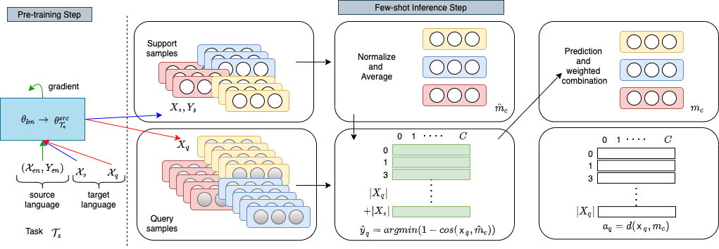
Figure 2: Training flow diagram of nearest neighbour few-shot learning for cross-lingual NLP. In the Pre-training Step we train a language model $\theta_{lm}$ on the source language (en) data $(\mathcal{X}_{src},\mathcal{Y}_{src})$ to get $\theta_{\mathcal{T}_{s}}^{src}$. In Few-Shot Inference Step, we apply forward propagation on the $\theta_{\mathcal{T}_{s}}^{src}$ model using support input samples $\mathcal{X}_{s}$ and $\mathcal{X}_{q}$ and get the latent representations $X_{s}$ and $Y_{s}$. Using $X_{s}$, we apply normalization and calculate $m_{c}$. We then use both $X_{s}$ and $X_{q}$, and compute the unary term $a_{q}$, which in turn gives the label distribution of the query samples (see in Alg. Few Shot Inference. line #14-15 ).

Transduction. We apply prototypical rectification (proto-rect) Liu et al. (2019) on the extracted features of LM. In the rectification step, to compute $m_{c}$ (in Alg.1), initially, we obtain the mean representation for each of the support classes by taking the weighted combination of $X_{s}$ and $X_{q}$. Finally, we calculate predictions on the query set using equation 3. We also present our proposed NNFS inference in Figure 2 in the Appendix.

3 Experimental Settings

3.1 Data

We use two standard multilingal datasets - XNLI Williams et al. (2018) (15 languages) and PAWS-X Zhang et al. (2019) (7 languages) to evaluate our proposed method. Additional details on languages and complexity of the task can be found in the Appendix. For few-Shot inference, we use samples from the target language development data to construct the support sets and the test data to construct the query sets.

Exp. Type	Resource	fr	es	de	el	bg	ru	tr	ar	vi	th	zh	hi	sw	ur	avg
$\theta_{\mathcal{T}_{s}}^{src}$ = Finetuned-XLM-R-large with XNLI dataset
Zero-Shot	en	83.1	84.8	83.0	82.2	83.4	80.1	78.8	78.8	80.1	78.1	79.4	76.7	72.7	72.9	79.6
NN	en+fs-3.5	83.0	84.6	82.7	82.0	83.3	80.3	78.9	79.2	80.2	78.3	79.5	76.6	71.9	73.0	79.5
+proto-rect	en+fs-3.5	83.7	85.2	83.5	82.7	84.1	81.2	79.8	80.3	81.2	79.4	80.4	77.7	73.5	74.4	80.5
+norm	en+fs-3.5	83.1	84.6	82.8	82.1	83.5	80.4	79.0	79.3	80.4	78.5	79.6	76.6	71.8	73.0	79.6
+proto-rect	en+fs-3.5	83.8	85.2	83.4	82.8	84.2	81.3	79.8	80.2	81.3	79.4	80.3	77.7	73.2	74.2	80.5
Fine-tuning (full)	en+fs-3.5	83.2	84.6	82.9	82.2	83.5	80.8	79.2	79.5	80.5	78.6	80.2	77.0	72.6	74.0	79.9
Fine-tuning (head)	en+fs-3.5	83.2	84.9	83.2	82.3	83.5	80.4	79.0	79.1	80.3	78.4	79.6	76.9	72.9	73.2	79.8

Table 1: Few-shot XNLI accuracy results across 14 languages with average improvements for each of the methods. All the confidence interval is less than .07 in the experiments. ”fs-3.5” means 3-way-5-shot learning.

Exp. Type	Resource	de	es	fr	ja	ko	zh	avg
$\theta_{\mathcal{T}_{s}}^{src}$ = Finetuned-XLM-R-large with PAWS-X dataset
Zero-Shot	en	89.8	89.6	90.5	78.8	78.6	81.9	84.9
NN	en+fs-2.5	89.8	89.8	90.6	79.8	80.4	82.5	85.5
+proto-rect	en+fs-2.5	90.3	90.2	91.0	80.5	81.2	83.3	86.1
+norm	en+fs-2.5	90.0	90.2	90.8	79.9	80.7	82.7	85.7
+proto-rect	en+fs-2.5	90.4	90.6	91.2	80.5	81.3	83.5	86.3
Fine-tuning (full)	en+fs-2.5	88.9	89.1	89.6	79.2	79.7	82.0	84.7
Fine-tuning (head)	en+fs-2.5	90.0	89.8	90.7	79.3	79.5	82.1	85.3

Table 2: Few-shot PAWS-X acc. results across 6 languages. Here in Resource column, ”en” indicates model is trained with full English training data. fs-2.5 means 2-way-5-shot learning.

Exp. Type	Resource	en	de	es	fr	ja	ko	zh	avg
$\theta_{\mathcal{T}_{s}}^{src}$ = Finetuned-XLM-R-large with XNLI dataset
Zero-Shot	en	41.4	43.5	44.1	43.8	46.0	46.7	44.4	44.3
NN	en+fs-2.5	71.5	66.8	65.2	66.6	60.1	58.8	61.8	64.4
+proto-rect	en+fs-2.5	70.5	66.1	65.1	66.2	60.0	58.6	61.6	64.0
+norm	en+fs-2.5	72.2	67.8	66.1	67.2	60.8	59.7	62.5	65.2
+proto-rect	en+fs-2.5	72.0	67.5	65.9	66.7	61.0	59.5	62.8	65.0
Fine-tuning (full)	en+fs-2.5	64.4	59.4	58.3	59.6	54.0	53.7	54.8	57.7
Fine-tuning (head)	en+fs-2.5	48.2	47.9	48.3	48.2	47.7	48.2	46.8	47.9

Table 3: PAWS-X accuracy results for cross-task experiments across 6 languages. For this experiment, we fine-tuned XLM-R LM using the XNLI task and then applied few-shot inference on the PAWS-X task.

3.2 Fine-tuning

We use XLMR-large Conneau et al. (2020) as our pre-trained language model $\theta_{lm}$ and perform standard fine-tuning using labeled English data to adapt it to task model $\theta_{\mathcal{T}_{s}}^{src}$. We tune the hyper-parameters using English development data and report results using the best performing model (optimal hyper-parameters have been enlisted in the appendix). We train our model using 5 different seeds and report average results across them. We use the same optimal hyper-parameters to fine-tune on the target languages. As baseline we add two additional fine-tuning named head and full. Fine-tuning full means all the parameters of the model are updated. This is very unlikely in Few-shot scenarios. Fine-tuning head means only the parameters of the last linear layer are updated.

3.3 Evaluation Setup

Nooralahzadeh et al. (2020) and Lauscher et al. (2020) used 10 and 5 different seeds to measure the few-shot performance. As few-shot learning involves randomly selecting small support sets, results may vary greatly from one experiment to the next, and hence may not be reliable Le et al. (2020). In computer vision, episodic testing Ravi and Larochelle (2017a); Li et al. (2019); Ziko et al. (2020) is often used for evaluating few-shot experiments. Each episode is composed of small randomly selected support and query sets. Model’s performance on each episode is noted, and the average performance score, alongside the confidence interval (95%) across all episodes are reported. To the best of our knowledge, episodic testing has not been leveraged for cross-lingual few-shot learning in NLP.

We evaluate our approach using 300 episodes per seed model $\theta_{\mathcal{T}_{s}}^{src}$ totalling 1500 episodic testing and report their average scores. For each episode, we perform C-way-N-shot inference. For 2-way-5-shot setting, for instance, we randomly select 15 query samples per class, and $2\times 5$ number of support samples. For XNLI and PAWS-X, we use $3$ and $2$ as the value of C, respectively. Our episodic testing approach has been detailed further in the Episodic Algorithm of the Appendix.

3.4 Results and Analysis

After training the model with the source language samples (i.e. labeled English data), we perform additional fine-tuning using $C$-way-5-shot target language samples. Finally, we perform our proposed NNFS inference.

The fine-tuning baseline using limited target language samples result in small but non-significant improvements over the zero-shot baseline. The NNFS inference approach, however, resulted in performance gains using only 15 (3-way-5-shot) and 10 (2-way-5-shot) support examples for both XNLI and PAWS-X tasks. When compared to the few-shot baseline, we got an average improvement of 0.6 on XNLI (table 4) and 1.0 on PAWS-X (table 5). At first we experimented with 3-shot support samples but did not observe any few-shot capability in the model. We also experimented with 10-shot setup and found similar improvements of NNFS on top of the Fine-tuning baseline (results have been added to the Appendix). Interestingly, for both cases, we observed higher performance gains on low resource languages.

To further evaluate the effectiveness of our model, we tested it in a cross-task setting. We first trained the model on XNLI (EN data) and then used NNFS inference on PAWS-X. Table 3 demonstrates an impressive average performance gain of +7.3 across all PAWS-X languages, over the fine-tuning baseline.

In addition to that, NNFS inference approach is fast. When compared to the zero-shot inference ($1\textsc{x}$), our approach takes only $\approx 1.36-1.7\textsc{x}$ time of computation cost compared to the finetuning time which takes $\approx 38-40\textsc{x}$. Table 6 in appendix shows the inference time details on both tasks.

4 Conclusion

The paper proposes a nearest neighbour based few-shot adaptation algorithm accompanied by a necessary evaluation protocol. Our approach does not require updating the LM weights and thus avoids over-fitting to limited samples. We experiment using two classification tasks and results demonstrate consistent improvements over finetuning not only across languages, but also across tasks.

Appendix A Appendices

A.1 Decision choice for Episodic Testing

In the traditional testing framework, we sample a batch from the dataset and calculate the batch’s prediction. Finally, accumulate all the predictions to calculate the score of the evaluation metric. However, Few-shot experiments are quite unpredictable because of the following two reasons,

• Support set: Per class sampling strategy of the support set is random. In a few shot experiments, we perform inference on the test dataset utilizing support-samples. For a different support set, the prediction may vary drastically. However, taking few samples (ie., 10 out of 2500 or 15 out of 2000) and doing experiments 5-10 times doesn’t reflect the true potential of a few-shot algorithm.

  

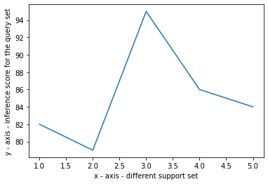
  Figure 1: For a same query set result varies because of different support set.

• Transductive inference: On the contrary, for a few shot experiments, algorithms often perform transductive inference. In transductive inference, predictions may vary based on the combination of the query samples. Hence it is challenging to benchmark the few shot algorithms with the traditional testing framework.

In Episodic testing, we randomly sample a query set and support set from the dataset and perform few-shot experiments. We perform the experiments until we get a low confidence-interval (95%). In this way, we may iterate over the test dataset 5-10 times more. However, it is not affected by the above problems mentioned and can benchmark any few-shot algorithm properly.

Algorithm 2 Episodic Testing

Input: Model $\theta_{\mathcal{T}_{s}}^{src}$ trained using the source language, transductive parameter $\lambda$, mean representation of train/dev samples $m_{s}$, a threshold value $eps$, a multiplier $\tau$, input data ($C$-way-$N$-shot)
Output: Average $\bar{s}$ score and the confidence interval $\partial$

1:$s_{e}=\phi$ $\triangleright$ score list for all the episodes.

2:for $e\in[1:totEpisode]$ do

3:     /* Random sampling */

4:     /* Randomly select $C$ number of classes */

5:     MetaClass = SelectRandomClasses($C$)

6:     /*bs = Batch Size*/

7:     $\mathcal{X}_{s},\mathcal{Y}_{s}$ = SupportIterator.next(bs=($C$-way-$N$ shot)) $\triangleright$ Iterator $\in$ MetaClass.

8:     $\mathcal{X}_{q}$ = QueryIterator.next(bs=($C$-way-$N\times\tau$ shot)) $\triangleright$ Iterator $\in$ MetaClass.

9:     /* Perform Inference using Respective few-shot algorithm. */

10:     $\mathcal{Y}_{q}$ = FewShotInference($\theta_{\mathcal{T}_{s}}^{src},(\mathcal{X}_{s},\mathcal{Y}_{s}),(\mathcal{X}_{q}),\lambda,m_{s},eps$) $\triangleright$ Using Alg. Few Shot Inference.

11:     $s$ = CalcScore($\mathcal{Y}_{q}$)

12:     $s_{e}\ \ =\ \ s_{e}\ \ \cup\ \ \{s\}$

13:$\bar{s}$, $\partial$ = Average($s_{e}$), ConfidenceInterval($s_{e}$)

14:Return $\bar{s}$, $\partial$

A.2 Extended Dataset

XNLI

We use XNLI dataset Conneau et al. (2018) which extends the MultiNLI dataset Williams et al. (2018) to 15 languages. MultiNLI dataset contains sentences from 10 different genres. The objective is to identify if a premise entails with the hypothesis. It is a crowd sourced 3-class classification dataset covering 14 languages that have been translated from English. These locales include French (fr), Spanish (es), German (de), Greek (el), Bulgarian (bg), Russian (ru), Turkish (tr), Arabic (a), Vietnamese (vi), Thai (th), Chinese (zh), Hindi (hi), Swahili (sw), and Urdu (ur). It comes with human translated dev and test splits. The dataset is balanced and contains 392702, 2490 and 5010 numbers of train, dev and test instance for each of the language, respectively.

PAWSX

Given a pair of sentences, the objective of PAWS (Paraphrase Adversaries from Word Scrambling) (Zhang et al., 2019) is to classify if the pair is a paraphrase or not. PAWS-X dataset contains six topologically different languages that have been machine translated from English. These include French (fr), Spanish (es), German (de), Korean (ko), Japanese (ja), and Chinese (zh). Similar to XNLI, it also comes with human translated dev and test split.

Challenges

Both datasets posses different challenges. NLI task requires rich and a high level of factual understanding of the text. The PAWS task, on the other hand, contains pairs of sentences that usually have a high lexical overlap and may/may not be paraphrases. We use accuracy as the evaluation metric for both datasets.

10 Shot results

For reference we have added 10 shot experiment for XNLI and PAWSX dataset with same setup as Table 1 and Table 2 of main paper.

Exp. Type	Resource	fr	es	de	el	bg	ru	tr	ar	vi	th	zh	hi	sw	ur	avg
$\theta_{\mathcal{T}_{s}}^{src}$ = Finetuned-XLM-R-large with XNLI dataset
Zero-Shot	en	83.1	84.8	83.0	82.1	83.3	80.2	78.9	78.7	80.1	78.1	79.5	76.7	72.5	73.0	79.6
NN	en+fs-3.10	83.4	85.0	83.1	82.5	83.8	80.9	79.5	79.8	80.8	79.2	80.3	77.4	72.9	74.0	80.2
NN+proto-rect	en+fs-3.10	83.8	85.3	83.6	82.8	84.1	81.2	79.9	80.4	81.3	79.6	80.7	78.1	73.6	74.7	80.6
NN+norm	en+fs-3.10	83.5	85.0	83.2	82.6	83.8	81.1	79.6	79.8	81.0	79.3	80.3	77.5	73.0	74.0	80.3
NN+norm+proto-rect	en+fs-3.10	83.8	85.2	83.6	82.8	84.2	81.4	80.0	80.4	81.4	79.7	80.7	78.1	73.5	74.6	80.7
Fine-tuning (full)	en+fs-3.10	83.2	84.5	82.9	82.5	83.7	81.2	79.5	79.8	80.8	78.9	80.5	77.3	72.6	74.2	80.1
Fine-tuning (head)	en+fs-3.10	83.3	85.0	83.2	82.4	83.5	80.6	79.2	79.4	80.5	78.6	79.9	77.2	72.8	73.6	79.9

Table 4: 10-shot XNLI accuracy results across 14 languages with average improvements for each of the methods. All the confidence interval is less than .07 in the experiments.

Exp. Type	Resource	de	es	fr	ja	ko	zh	avg
$\theta_{\mathcal{T}_{s}}^{src}$ = Finetuned-XLM-R-large with PAWS-X dataset
Zero-Shot	en	89.8	89.6	90.6	78.8	78.4	81.8	84.8
NN	en+fs-2.10	90.0	90.1	90.8	80.2	80.7	83.2	85.8
NN+proto-rect	en+fs-2.10	90.3	90.3	91.2	80.5	81.2	83.5	86.2
NN+norm	en+fs-2.10	90.1	90.4	91.1	80.3	81.0	83.3	86.0
NN+norm+proto-rect	en+fs-2.10	90.4	90.7	91.4	80.7	81.5	83.7	86.4
Fine-tuning (full)	en+fs-2.10	89.4	89.6	90.1	79.9	80.6	82.6	85.4
Fine-tuning (head)	een+fs-2.10	90.1	90.1	91.0	79.9	79.8	82.5	85.6

Table 5: 10-shot PAWS-X acc. results across 6 languages. Here in Resource column, ”en” indicates model is trained with full english training data.

A.3 Hyperparameters and Resource Description

We used 8 V100 GPUs (amazon p3.16xlarge) to run all experiments. The hyper-parameters of the best performing model are enlisted in Table 6. In the pretrained language model finetuning, We use (1e-5, 3e-5, 5e-5, 7.5e-6 ,5e-6) boundary values to search for proper learning rate.

Hyperparameter	Value
LM	XLMR-large
# of params	550M
learning rate	7.5e-6
Max Sequence Length	128
Per GPU batch size	8
Gradient accumulation step	2
Multi-GPU training	8
Effective batch size	128
Number of epoch	10
Warmup step in pre-training	6% of total number of steps
Total number of episodic test	1000
finetuning batch-size	16
finetuning learning rate	7.5e-6
finetuning schedueler	constant scheduler

Table 6: Optimal hyper-parameter settings.

Exp. Type	PAWSX		XNLI
	fs-2.5	fs-2.10	fs-3.5	fs-3.10
Zero-Shot	1x	1x	1.35x	1x
NN	1.36x	1.71x	1.35x	1.66x
+proto-rect	1.37x	1.71x	1.35x	1.67x
+norm	1.36x	1.71x	1.35x	1.66x
+proto-rect	1.37x	1.71x	1.35x	1.67x
Fine-tuning (full)	22.44x	41.86x	21.01x	38.69
Fine-tuning (head)	20.48x	38.02x	19.24x	35.17

Table 7: Inference time for each of the task.

Appendix B Reproducibility Settings and Notes

• $python_{3.6.13}$. $Pytorch_{1.7.1}$, $CUDA_{10.2}$, $cuDNN_{7605}$

• $transformers_{4.6.0}$

• Average runtime: See table 7.

References

- Bari et al. (2020) M Saiful Bari, Tasnim Mohiuddin, and Shafiq Joty. 2020. Multimix: A robust data augmentation framework for cross-lingual nlp.
- Chelsea Finn (2017) Sergey Levine Chelsea Finn, Pieter Abbeel. 2017. Model-agnostic meta-learning for fast adaptation of deep networks.
- Chi et al. (2020) Zewen Chi, Li Dong, Furu Wei, Nan Yang, Saksham Singhal, Wenhui Wang, Xia Song, Xian-Ling Mao, Heyan Huang, and Ming Zhou. 2020. Infoxlm: An information-theoretic framework for cross-lingual language model pre-training.
- Conneau et al. (2020) Alexis Conneau, Kartikay Khandelwal, Naman Goyal, Vishrav Chaudhary, Guillaume Wenzek, Francisco Guzmán, Edouard Grave, Myle Ott, Luke Zettlemoyer, and Veselin Stoyanov. 2020. Unsupervised cross-lingual representation learning at scale. In Proceedings of the 58th Annual Meeting of the Association for Computational Linguistics, pages 8440–8451, Online. Association for Computational Linguistics.
- Conneau et al. (2018) Alexis Conneau, Guillaume Lample, Ruty Rinott, Adina Williams, Samuel R. Bowman, Holger Schwenk, and Veselin Stoyanov. 2018. XNLI: evaluating cross-lingual sentence representations. CoRR, abs/1809.05053.
- Fang et al. (2020) Yuwei Fang, Shuohang Wang, Zhe Gan, Siqi Sun, and Jingjing Liu. 2020. Filter: An enhanced fusion method for cross-lingual language understanding.
- Finn et al. (2017) Chelsea Finn, Pieter Abbeel, and Sergey Levine. 2017. Model-agnostic meta-learning for fast adaptation of deep networks. CoRR, abs/1703.03400.
- Gao et al. (2020) Silin Gao, Yichi Zhang, Zhijian Ou, and Zhou Yu. 2020. Paraphrase augmented task-oriented dialog generation.
- Jake Snell (2017) Richard S. Zemel Jake Snell, Kevin Swersky. 2017. Prototypical networks for few-shot learning.
- K et al. (2020) Karthikeyan K, Zihan Wang, Stephen Mayhew, and Dan Roth. 2020. Cross-lingual ability of multilingual {bert}: An empirical study. In International Conference on Learning Representations.
- Keung et al. (2019) Phillip Keung, yichao lu, and Vikas Bhardwaj. 2019. Adversarial learning with contextual embeddings for zero-resource cross-lingual classification and ner. Proceedings of the 2019 Conference on Empirical Methods in Natural Language Processing and the 9th International Joint Conference on Natural Language Processing (EMNLP-IJCNLP).
- Koch (2015) Gregory R. Koch. 2015. Siamese neural networks for one-shot image recognition.
- Lample and Conneau (2019) Guillaume Lample and Alexis Conneau. 2019. Cross-lingual language model pretraining. Advances in Neural Information Processing Systems (NeurIPS).
- Lauscher et al. (2020) Anne Lauscher, Vinit Ravishankar, Ivan Vulić, and Goran Glavaš. 2020. From zero to hero: On the limitations of zero-shot cross-lingual transfer with multilingual transformers.
- Le et al. (2020) Canyu Le, Zhonggui Chen, Xihan Wei, Biao Wang, and Lei Zhang. 2020. Continual local replacement for few-shot learning.
- Li et al. (2019) Hongyang Li, David Eigen, Samuel Dodge, Matthew Zeiler, and Xiaogang Wang. 2019. Finding task-relevant features for few-shot learning by category traversal. CoRR, abs/1905.11116.
- Liu et al. (2019) Jinlu Liu, Liang Song, and Yongqiang Qin. 2019. Prototype rectification for few-shot learning. CoRR, abs/1911.10713.
- Luo et al. (2020) Fuli Luo, Wei Wang, Jiahao Liu, Yijia Liu, Bin Bi, Songfang Huang, Fei Huang, and Luo Si. 2020. Veco: Variable encoder-decoder pre-training for cross-lingual understanding and generation.