On the extreme eigenvalues of the precision matrix of the nonstationary autoregressive process and its applications to outlier estimation of panel time series

Abstract

This paper investigates the structural change of the coefficients in the autoregressive process of order one by considering extreme eigenvalues of an inverse covariance matrix (precision matrix). More precisely, under mild assumptions, extreme eigenvalues are observed when the structural change has occurred. A consistent estimator of extreme eigenvalues is provided under the panel time series framework. The proposed estimation method is demonstrated with simulations.

Keywords and phrases: Autoregressive process, empirical sepctral distribution, extreme eigenvalues, panel time series, structural change model.

1 Introduction

Consider the autoregressive model

$$y_{t}=\rho_{t}y_{t-1}+z_{t}\qquad t\geq 1,$$ (1.1)

where the initial state $y_{0}=0$ and $\{z_{t}\}$ is a white noise process with variance $\mathbb{E}[z_{t}^{2}]=\sigma^{2}>0$ and $z_{t}$ is uncorrelated with $y_{0},y_{1},...,y_{t-1}$. If the AR coefficients $\{\rho_{t}\}$ are constant with absolute value less than 1, then, $\{y_{t}\}$ limits to a (causal) second order stationary autoregressive process of order 1, henceforth denoted as a stationary AR$(1)$ process.

We suppose that the AR coefficients have the following structure

$$\rho_{t}=\rho+\sum_{j=1}^{m}\varepsilon_{j}I_{E_{j}}(t)\qquad t\geq 1,$$ (1.2)

where $\rho\in(-1,1)/\{0\}$, $m\geq 0$, nonzero constants $\{\varepsilon_{j}\}_{j=1}^{m}$, disjoint intervals $\{E_{j}\}_{j=1}^{m}$, and $I_{A}(t)$ is an indicator function takes value one when $t\in A$ and zero elsewhere. We use a convention $\sum_{1}^{0}=0$. When $m=0$, (1.2) corresponds to a stationary AR$(1)$ model (in an asymptotic sense), we refer to it as a null model. When $m>0$, a process $\{y_{t}\}$ is no longer stationary, and the non-stationarity is due to the structural change of the coefficients. We refer to this case as an alternative model or the Structural Change Model (SCM).

Given $n$ observations $\underline{y}_{n}=(y_{1},...,y_{n})^{\prime}$ where the AR coefficients satisfy (1.2), there is a large body of literature on constructing a test for $H_{0}:m=0$ versus $H_{A}:m>0$. Many change point detection methods of time series data are based on the cumulative sum (CUSUM; Page (1955)) which was first developed to detect change in the mean of mean structure of independent samples. Using a similar scheme from Page (1955), Gombay (2008) and Gombay and Serban (2009) tested the structural change for parameters of finite order autoregressive processes. Several diverse methods of the change point detection time series can be found in Bagshaw and Johnson (1977); Davis et al. (1995); Lee et al. (2003); Shao and Zhang (2010); Aue and Horváth (2013); and Lee and Kim (2020). Test procedures from the aforementioned literature are based on the likelihood ratio and/or Kolmogorov-Smirnov type test. To achieve a statistical power for those test statistics, it is necessary to assume that

$$\lim_{n\rightarrow\infty}|E_{j}|/n=\tau_{j}\in(0,1)$$

where $|E_{j}|$ is a segment length of $E_{j}$. That is, the segment of changes is sufficiently large enough to detect the changes in structure, otherwise, the test will fail (see also Davis et al. (2006), page 225). However, in many real-world time series data (especially economic data), it is often more realistic to assume that the change occurs sporadically. In this case, we assume that $|E_{j}|=o(n)$, or, in an extreme case, $|E_{j}|$ is finite as $n\rightarrow\infty$. To detect these abrupt changes or the “outliers”, Fox (1972) considered two types of outliers in the Gaussian autoregressive moving average (ARMA) model—the Addition Outlier (AO) and Innovational Outlier (IO) — and proposed a likelihood ratio test to detect these. The concept of the AO and IO in a time series model was later generalized by several authors, e.g., Hillmer et al. (1983); Chang et al. (1988); Tsay (1988), all of whom investigated outliers of the disturbed autoregressive integrated moving average (ARIMA) model $\{Y_{t}\}$

$$Y_{t}=\omega_{0}\frac{\omega(B)}{\delta(B)}e_{t}^{(d)}+Z_{t}$$ (1.3)

where $\{Z_{t}\}$ is an unobserved Gaussian ARIMA process, $\omega_{0}$ is a scale, $\omega(\cdot)$ and $\delta(\cdot)$ are polynomials with zeros outside the unit circle, $B$ is a backshift operator, and $e_{t}^{(d)}$ is either deterministic

$$e_{t}^{(d)}=I_{\{d\}}(t)$$

or stochastic

$$e_{t}^{(d)}=0~{}~{}(t<d)\quad\text{and}\quad\{e_{t}^{(d)}:t\geq d\}:i.i.d.\text{ mean zero random variables}.$$

The deterministic disturbance $\omega_{0}(\omega(B)/\delta(B))e_{t}^{(d)}$ in (1.3) impacts the expectation of $\{Y_{t}\}$, whereas the stochastic disturbance is used to model change in variance. More applications of the disturbed ARIMA model and outlier detection can be found in Harvey and Koopman (1992) (using auxiliary residuals from the Kalman filter), McCulloch and Tsay (1993) (using Bayesian inference), and De Jong and Penzer (1998); Chow et al. (2009) (using a state-space model). However, as far as we are aware, there is no clear connection between the SCM in (1.2) and the disturbed ARIMA model in (1.3). Indeed, there is no deterministic or stochastic disturbance of form $\omega_{0}(\omega(B)/\delta(B))e_{t}^{(d)}$ that yields the model (1.2) in general case.

The main contribution of this paper is to provide a new approach to characterize the structural change in the coefficients, which is particularly useful when $|E_{j}|$ is finite. The main ingredient of our approach is the eigenvalues of the inverse covariance matrix (precision matrix). More precisely, let

$$A_{n}=[\mathrm{var}(\underline{y}_{n})]^{-1}\in\mathbb{R}^{n\times n}$$ (1.4)

be a precision matrix of $\underline{y}_{n}$ (an explicit form of $A_{n}$ is given in Lemma 2.1). Since $A_{n}$ is symmetric and positive definite, we let $0<\lambda_{1}(A_{n})\leq...\leq\lambda_{n}(A_{n})$ are the eigenvalues of $A_{n}$ in decreasing order (note that in some papers, $\lambda_{1}(A_{n})$ is defined as the largest eigenvalue, but for notational convenience, we denote $\lambda_{1}(A_{n})$ to be the smallest eigenvalue). To motivate the behavior of the eigenvalues in the SCM, we consider the following null model and the SCM

$$\text{Null}:\rho_{t}=0.3\quad v.s.\quad\text{SCM}:\rho_{t}=0.3+0.2I_{50}(t)\qquad 1\leq t\leq 1000.$$ (1.5)

That is, on the SCM, only one coefficient ($\rho_{50}$) differs from other coefficients.

Figure 1 shows a single realization of $\underline{y}_{n}$ under the null model (left panel) and the alternative model (right panel). We use i.i.d. standard Normal errors, $\{z_{t}\}$, to generate the time series. Since the magnitude of change in the SCM is not pronounced, it is hardly noticeable the structural change in the SCM.

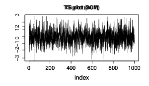
Figure 1: Sample Gaussian time series trajectories for the null model (left) and the SCM (right). Vertical dashed line is where the structural change occurs in the SCM.

Figure 2 compares the histogram of the eigenvalues of precision matrix under the null model (right panel) and the SCM (left panel). There are two important things to note in Figure 2:

• The distribution of eigenvalues under the null and alternative are almost identical.

• Under the alternative (left panel), we observe two outliers, marked with crosses, one each on the left and right side, which are apart from the eigenvalue bundle.

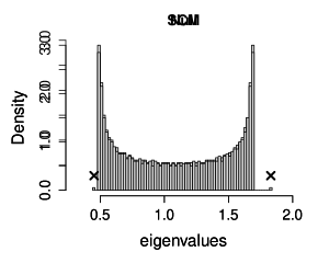
Figure 2: Histogram of the eigenvalues of the precision matrix in model (1.5). Left: the null, right: the SCM. Crosses on the right panel indicate the outliers.

It is worth noting that the second observation (outlied eigenvalues) is referred to as spiked eigenvalues in the random matrix literature (when the covariance or inverse covariance matrices are random) and has received much attention in the past two decades in both probability thoery and Statistics. Selections include Johnstone (2001) (distribution of the largest eigenvalue in PCA), Baik and Silverstein (2006); El Karoui (2007); Paul (2007) (eigenvalues of the large sample covariances), Zhang et al. (2018)(unit root testing using the largest eigenvalues), and Steland (2020) (CUSUM testing for the spiked covariance model), to name a few.

To rigorously argue the observations found in Figure 2, we first define the empirical spectral distribution (ESD) of the matrix $A_{n}$

$$\mu_{A_{n}}:=\frac{1}{n}\sum_{i=1}^{n}\delta_{\lambda_{i}(A_{n})},$$ (1.6)

where $\delta_{x_{0}}$ is a Dirac measure of center $x_{0}$. In Section 2, we study the asymptotic spectral distribution (ASD) of $\mu_{A_{n}}$ when the AR coefficients satisfy (1.2). Especially, in Section 2.2, we show that if $|E_{j}|/n\rightarrow 0$ for all $1\leq j\leq m$, then ASD of a precision matrix of SCM is the same as the ASD of the null model. We also derive the explicit formula for the Stieltjes transformation (see Tao (2012), Section 4.2.3. and the references therein) of the common ASD in the Appendix (see Proposition A.1), which is an important element in the development of the theoretical results in the following sections.

In Section 3, we investigate the outliers of ESD. Given the sequence of probability measures $\{\mu_{A_{n}}\}$, we define the outliers of $\{\mu_{A_{n}}\}$, denoting $out(\{A_{n}\})$. In Section 3.1, we show that

$$out(\{A_{0,n}\})=\emptyset,$$

where $A_{0,n}$ denotes the precision matrix of $\underline{y}_{n}$ under the null model. That is, as expected on the left panel of Figure 2, the ESD of the null model does not have an outlier. Next, we turn our attention to the outliers of the alternative model. In Sections 3.2–3.4, we show that $out(\{A_{n}\})\neq\emptyset$ for all SCM. This is true even if there is a single change in (1.2), e.g. an alternative model in (1.5). We also show that the element of $out(\{A_{n}\})$ is a solution of a determinantal equation. Therefore, for the simplest case where $m=1$ and $|E_{1}|=1$ (a single structural change), we can obtain an explicit form for outliers. In general case, we can numerically obtain $out(\{A_{n}\})$.

In Section 4, we discuss the identifiability of parameters in the SCM. In Section 5, we provide a consistent estimator of $out(\{A_{n}\})$ under the panel time series framework and we demonstrate the performance of an estimator through some simulations in Section 6. In Section 7, we discuss the extreme eigenvalues for the structural change in variances (heteroscedasticity model).

Lastly, additional properties of an ASD and the proofs can be found in the Appendix.

2 Asymptotic Spectral Distribution

2.1 Preliminaries

We first will introduce some notation and terminology used in the paper. For the SCM of form $\rho_{t}=\rho+\sum_{j=1}^{m}\varepsilon_{j}I_{E_{j}}(t)$, disjoint intervals $\{E_{j}\}_{j=1}^{m}$ can be written

$$E_{j}=[k_{j},(k_{j}+h_{j}-1)]=\{x:k_{j}\leq x\leq k_{j}+h_{j}-1,x\in\mathbb{N}\}\qquad 1\leq j\leq m$$

where $1\leq k_{1}<k_{1}+h_{1}-1<k_{2}<...<k_{m}<k_{m}+h_{m}-1\leq n$. We refer to $m$ as the number of changes; $k_{j}$ as the $j$th break point; $h_{j}$ as the $j$th length of change; and $\varepsilon_{j}$ as the $j$th magnitude of change. In particular, when $m=1$ and $h_{1}=1$, we omit the subscription in $k_{1}$ and $\varepsilon_{1}$ and write

$$\rho_{t}=\rho+\varepsilon I_{\{k\}}(t).$$ (2.1)

We call (2.1) the single structural change model (single SCM). Let $A_{n}$ be a general precision matrix of $\underline{y}_{n}$. Sometimes, it will be necessary to distinguish the null and alternative model. In this case, $A_{0,n}$ and $B_{n}$ refer to the precision matrix of the $n$-section of the null and alternative model, respectively.

For a real symmetric matrix $A\in\mathbb{R}^{n\times n}$, $spec(A)=\{\lambda_{i}(A)\}_{i=1}^{n}$ is a spectrum of $A$. For $|\rho|<1$, we make an extensive use of the following notation

$$a_{\rho}=(1-|\rho|)^{2}\qquad\text{and}\qquad b_{\rho}=(1+|\rho|)^{2}.$$

Lastly, $\wedge$ and $\vee$ refer to minimum and maximum, respectively and $\stackrel{{\scriptstyle P}}{{\rightarrow}}$ and $\stackrel{{\scriptstyle\mathcal{D}}}{{\rightarrow}}$ refer to the convergence in probability and distribution respectively.

The following lemma gives an explicit form of $A_{n}$.

Lemma 2.1

Let $A_{n}$ be a precision matrix of $\underline{y}_{n}=(y_{1},...,y_{n})^{\prime}$, where $\{y_{i}\}_{i=1}^{n}$ follows the recursion (1.1). Then, $\{A_{n}\}$ are symmetric tri-diagonal matrices with entries

$$[A_{n}]_{i,j}=\left\{\begin{array}[]{ll}1&i=j=n\\ 1+\rho_{i+1}^{2}&i=j<n\\ -\rho_{i\vee j}&|i-j|=1\\ 0&o.w.\end{array}\right..$$ (2.2)

PROOF. See Appendix C $\Box$

From the above lemma, we can define the positive-valued eigenvalues of $A_{n}$ and the ESD in (1.6) is well-defined on the positive real line.

2.2 Asymptotic Spectral Distribution under the null and alternative model

Let $A_{0,n}$ be a precision matrix of the null model where the AR coefficients are constant to $\rho\in(-1,1)/\{0\}$. Then, by Lemma 2.1, $A_{0,n}$ has the following form

$$A_{0,n}=\begin{pmatrix}1+\rho^{2}&-\rho&0&\cdots&0\\ -\rho&1+\rho^{2}&-\rho&\ddots&\vdots\\ 0&-\rho&\ddots&\ddots&0\\ \vdots&\ddots&\ddots&1+\rho^{2}&-\rho\\ 0&\cdots&0&-\rho&1\\ \end{pmatrix}\in\mathbb{R}^{n\times n}.$$ (2.3)

Note that $A_{0,n}$ is “nearly” (not “exactly”) a Toeplitz matrix due to the element on the bottom right corner. Therefore, for technical reasons, we define the slightly perturbed Toeplitz matrix

$$\widetilde{A}_{0,n}=A_{0,n}+\rho^{2}E_{n},$$ (2.4)

where $E_{n}=\mathrm{diag}(0,...,0,1)$ a $n\times n$ diagonal matrix. Then, by Stroeker (1983), Proposition 2, we obtain an explicit form for the entire set of eigenvalues and the corresponding normalized eigenvectors. When $\rho>0$, the $k$th (smallest) eigenvalue is

$$\lambda_{k}(\widetilde{A}_{0,n})=1-2\rho\cos\left(\frac{k\pi}{n+1}\right)+\rho^{2}\qquad 1\leq k\leq n,$$ (2.5)

and the corresponding normalized eigenvector $\widetilde{u}_{k}=(\widetilde{u}_{1k},...,\widetilde{u}_{nk})^{\prime}$ is

$$\widetilde{u}_{jk}=\sqrt{\frac{2}{n+1}}\sin\left(\frac{kj\pi}{n+1}\right)\qquad 1\leq j,k\leq n.$$ (2.6)

The above expression is for $\rho>0$, and when the $\rho<0$, eigenstructure has the same expressions but is arranged in the reverse order.

Since $\widetilde{A}_{0,n}$ is a Toeplitz matrix of finite order, we can directly apply the Szegö limit theorem (see e.g. Grenander and Szegö (1958), Chapter 5) to $\{\widetilde{A}_{0,n}\}$.

Lemma 2.2 (Szegö limit theorem)

Let $\widetilde{A}_{0,n}$ as defined in (2.5) and $\mu_{\widetilde{A}_{0,n}}$ be an ESD of $\widetilde{A}_{0,n}$. Then,

$$\mu_{\widetilde{A}_{0,n}}\stackrel{{\scriptstyle\mathcal{D}}}{{\rightarrow}}\mu_{\rho}$$

for some probability measure $\mu_{\rho}$ on $\mathbb{R}$ with distribution

$$F_{\mu_{\rho}}(t)=\mu_{\rho}((-\infty,t])=\frac{1}{2\pi}\int_{0}^{2\pi}I_{(-\infty,t]}(1+\rho^{2}-2\rho\cos x)dx.$$ (2.7)

Moreover, $\mu_{\rho}$ is compactly supported where the lower and upper bound of the support are

$$a_{\rho}=\inf(supp(\mu_{\rho}))=(1-|\rho|)^{2}\qquad\text{and}\qquad b_{\rho}=\sup(supp(\mu_{\rho}))=(1+|\rho|)^{2},$$ (2.8)

where $supp(\mu_{\rho})$ is a support of $\mu_{\rho}$.

PROOF. (2.7) is immediately from the Szegö limit theorem. (2.8) is also clear since the range of $(1+\rho^{2}-2\rho\cos x)$ is $[(1-|\rho|)^{2},(1+|\rho|)^{2}]$. $\square$

From the above lemma, a slightly perturbed matrix of the null model has an ASD with known distribution. Our next interest is to find, if it exists, an ASD of the null and alternative models. Note that the structural change model in (1.2) also includes the null model by setting $m=0$. Therefore, it is enough to study the ASD of the model based on (1.2). The following theorem addresses the ASD of (1.2).

Theorem 2.1

Let $A_{n}$ be a precision matrix of an AR$(1)$ model where the AR coefficients satisfies (1.2). Define $\tau_{j}=\lim_{n\rightarrow\infty}h_{j}/n\in[0,1]$ where $h_{j}$ is the $j$th length of change. We assume that if $\tau_{j}>0$, then $|\rho+\varepsilon_{j}|<1$. Then,

$$\mu_{A_{n}}\stackrel{{\scriptstyle\mathcal{D}}}{{\rightarrow}}\big{(}1-\sum_{j=1}^{m}\tau_{j}\big{)}\mu_{\rho}+\sum_{j=1}^{m}\tau_{j}\mu_{\rho+\varepsilon_{j}},$$ (2.9)

$\mu_{\rho}$ is defined as in Lemma 2.2.

PROOF. See Appendix C. $\Box$

Some remarks are made on the ASD of the null and alternative models.

Remark 2.1

• By letting $m=0$, an ASD of the null model $A_{0,n}$ is

  $$\mu_{A_{0,n}}\stackrel{{\scriptstyle\mathcal{D}}}{{\rightarrow}}\mu_{\rho}.$$

• In the special case of the alternative model where $\tau_{j}=0$ for all $1\leq j\leq m$, an ASD of the alternative model $\{B_{n}\}$ is also $\mu_{B_{n}}\stackrel{{\scriptstyle\mathcal{D}}}{{\rightarrow}}\mu_{\rho}$.

3 Outliers of the Structural Change Model

In this section, we define the “outliers” of the sequence of measures and study the outliers of the SCM. Throughout the rest of the paper, we assume that $\sup_{j}h_{j}/n\rightarrow 0$ as $n\rightarrow\infty$. Then, by the Remark 2.1, the ASD of $\{A_{0,n}\}$(the null model) and $\{B_{n}\}$ (the SCM) are equivalent to $\mu_{\rho}$. However, this does not imply that $A_{0,n}$ and $B_{n}$ are not distinguishable. The simulation in Section 1 shows that two eigenvalues of $B_{n}$ are apart from the “common” distribution of $\mu_{\rho}$. However, for the null model, $A_{0,n}$, all the eigenvalues lie within the common distribution. Bearing this in mind, we formally define the “outlier” of the sequence of compactly supported measures.

Definition 3.1

Let $\{A_{n}\}$ be a sequence of Hermitian matrices, where $\mu_{A_{n}}\stackrel{{\scriptstyle\mathcal{D}}}{{\rightarrow}}\mu$ for some compactly supported deterministic measures on $\mathbb{R}$. Let $\overline{S}_{\mu}$ be the closure of the support of $\mu$. Then, the point $x\in\mathbb{R}$ is called an outlier of the sequence $\{A_{n}\}$ (or $\{\mu_{A_{n}}\}$), if it satisfies two conditions

$$\lim_{n\rightarrow\infty}\inf_{y\in spec(A_{n})}|x-y|=0$$ (3.1)

$$x\notin\overline{S}_{\mu}.$$ (3.2)

We denote $out(\{A_{n}\})$ the set of all outliers of $\{A_{n}\}$ (or $\{\mu_{A_{n}}\}$). Moreover, when the support of $\mu$ is an interval, i.e., $\overline{S}_{\mu}=[a,b]$, then we can define the set of left and right outliers

$$out_{L}(\{A_{n}\})=out(\{A_{n}\})\cup(-\infty,a)\qquad\text{and}\qquad out_{R}(\{A_{n}\})=out(\{A_{n}\})\cap(b,\infty)$$

respectively.

That is, the outliers are the limit point of the spectrum of $A_{n}$, which are not contained in the closure of the support of ASD. Therefore, if the support of ASD is an interval, the outliers are closely related to the extreme eigenvalues of $A_{n}$. The remaining part of this section discusses the outliers of $\{A_{0,n}\}$ and $\{B_{n}\}$ by studying the extreme eigenvalues.

3.1 Outliers of the null model

In this section, we study the outliers of the null model, $\{A_{0,n}\}$. From Lemma 2.2 and Remark 2.1(i), ASD of the null model has a support $[a_{\rho},b_{\rho}]$. The following lemma states the behavior of the extreme eigenvalues of $A_{0,n}$.

Lemma 3.1

Let $A_{0,n}$ be as defined in (2.3) and $a_{\rho}$ and $b_{\rho}$ be as defined in (2.8). Then, for fixed $j\geq 1$,

$$\lim_{n\rightarrow\infty}\lambda_{j}(A_{0,n})=a_{\rho}\qquad\text{and}\qquad\lim_{n\rightarrow\infty}\lambda_{n+1-j}(A_{0,n})=b_{\rho}.$$

PROOF. See Appendix C. $\Box$

Lemma 3.1 shows that under the null, the $j$th smallest and largest eigenvalue converges into the lower ($a_{\rho}$) and upper bound ($b_{\rho}$) of the support of an ASD, respectively. As a consequence of Lemma 3.1, the following theorem shows that there is no outlier of the null model.

Theorem 3.1

Let $A_{0,n}$ be as defined in (2.3). Then,

$$out(\{A_{0,n}\})=\emptyset.$$

PROOF. We first show $out_{L}(\{A_{0,n}\})=\emptyset$. Assume by contradiction, that we can find $x<a_{\rho}$ such that $x\in out_{L}(\{A_{0,n}\})$. Let $\delta=(a_{\rho}-x)/2>0$. Then, from (3.1), there exists an integer $N$ such that for all $n\geq N$, there exists $1\leq j(n)\leq n$ such that

$$|x-\lambda_{j(n)}(A_{0,n})|<\delta.$$

Therefore, for $n\geq N$, $\lambda_{1}(A_{0,n})\leq\lambda_{j(n)}(A_{0,n})<x+\delta=a_{\rho}-\delta$. Thus, $\lambda_{1}(A_{0,n})$ does not converge to $a_{\rho}$, which contradicts to Lemma 3.1. Therefore, $out_{L}(\{A_{0,n}\})=\emptyset$. Similarly, we can show $out_{R}(\{A_{0,n}\})=\emptyset$ and this proves the result. $\Box$

3.2 Outliers of the single Structural Change Model

In this section, we investigate the outliers of $B_{n}$ for the single SCM. Recall the single SCM has AR coefficients of the form $\rho_{t}=\rho+\varepsilon I_{\{k\}}(t)$, where we assume that $\rho\in(-1,1)$ and $\varepsilon$ are nonzero and fixed over $n$. To obtain the outliers, we require the following assumptions on the break point.

The break point $$k k\rightarrow\infty n\rightarrow\infty$$ is such that as . (3.3)

Next, we define the following functions of $\rho$ and $\varepsilon$

$$s=\frac{\rho\varepsilon(\varepsilon+2\rho)-\sqrt{\rho^{2}\varepsilon^{2}(\varepsilon+2\rho)^{2}+4\rho^{2}(\varepsilon+\rho)^{2}}}{2(\varepsilon+\rho)^{2}},$$

$$t=\frac{\rho\varepsilon(\varepsilon+2\rho)+\sqrt{\rho^{2}\varepsilon^{2}(\varepsilon+2\rho)^{2}+4\rho^{2}(\varepsilon+\rho)^{2}}}{2(\varepsilon+\rho)^{2}}.$$ (3.4)

The following theorem gives an explicit formula for $out(\{B_{n}\})$.

Theorem 3.2

Let $\{B_{n}\}$ be the precision matrix of single SCM described as in (2.1). Further, the break point $k$ satisfies (3.3). Then, we have the following dichotomies:

$$out_{L}(\{B_{n}\})=\left\{\begin{array}[]{ll}\emptyset&|\rho|\geq|\rho+\varepsilon|\\ \{m\}&|\rho|<|\rho+\varepsilon|\end{array}\right.\quad\text{and}\quad out_{R}(\{B_{n}\})=\left\{\begin{array}[]{ll}\emptyset&|\rho|\geq|\rho+\varepsilon|\\ \{M\}&|\rho|<|\rho+\varepsilon|\end{array}\right.$$

where $m$ and $M$ are

$$m = 1+\rho^{2}-\rho(s+s^{-1}),\quad M=1+\rho^{2}-\rho(t+t^{-1})\quad\text{for}\quad-1<\rho<0$$ (3.5)

$$m = 1+\rho^{2}-\rho(t+t^{-1}),\quad M=1+\rho^{2}-\rho(s+s^{-1})\quad\text{for}\quad 0<\rho<1$$ (3.6)

where $s,t$ are from (3.4).

PROOF. See Appendix C. $\Box$

Remark 3.1

1. Dichotomies in Theorem 3.2 show that if the magnitude of the AR coefficient at the break point ($|\rho+\varepsilon|$) is smaller than the original AR coefficient ($|\rho|$), then the effect of the change is absorbed in the overall effect, so we cannot observe an outlier. However, as we observed from the simulation result in the Introduction, if $|\rho+\varepsilon|>|\rho|$, then we observe exactly two outliers (one on the left and another on the right).

2. When the error variance $\mathbb{E}z_{t}^{2}=\sigma^{2}\neq 1$, the outliers $m$ and $M$ in Theorem 3.2 have the same form, but multiplied by $\sigma^{2}$.

3. Suppose the break point $k$ is fixed so that the condition (3.3) is not satisfied. Then, for $|\rho|<|\rho+\varepsilon|$, there exists $|c|<1$ (depends on $\rho$) such that

   $$out_{L}(\{B_{n}\})=m+O(|c|^{k})\qquad\text{and}\qquad out_{R}(\{B_{n}\})=M+O(|c|^{k})$$

   where $(m,M)$ is defined as in (3.5) (if $-1<\rho<0$) or (3.6) (if $0<\rho<1$). A proof can be found in the Appendix C, proof of Theorem 3.2, [Step7]. In practice, for a moderate AR coefficient value, e.g., $|\rho|=0.7$, $k>5$ is sufficiently large to approximate the outliers using $m$ and $M$.

The following corollary states the behavior of outliers when the magnitude of change dominates the original AR coefficient.

Corollary 3.1

Suppose the same notation and assumptions as those in Theorem 3.2 hold. If $|\rho|<|\rho+\varepsilon|$, then

$$\lim_{|\varepsilon|\rightarrow\infty}m=0\quad\text{and}\quad\lim_{|\varepsilon|\rightarrow\infty}\frac{M-b_{\rho}}{\varepsilon^{2}}=1.$$

PROOF. We assume $\rho>0$ (proof for $\rho<0$ is similar). Since $\lim_{|\varepsilon|\rightarrow\infty}t\rightarrow\rho$, then, $m\rightarrow 1+\rho^{2}-\rho(\rho+\rho^{-1})=0$ as $|\varepsilon|\rightarrow\infty$. This proves the first limit. To show the second limit, From (3.6),

$$M-b_{\rho}=-\rho(s+s^{-1}+2)=\rho\left(\frac{(\varepsilon+\rho)^{2}}{\rho^{2}}t-s+2\right)$$

Here we use the equation $st=-\rho^{2}(\rho+\varepsilon)^{-2}$. Finally, using that $\lim_{\varepsilon\rightarrow\infty}s=0$ and $\lim_{\varepsilon\rightarrow\infty}t=\rho$, it is straightforward to show $\varepsilon^{-2}(M-b_{\rho})\rightarrow 1$ as $\varepsilon\rightarrow\infty$. $\Box$

In the following two sections, we derive a general solution of outliers for the general SCM.

3.3 Outliers of the single interval Structural Change Model

As a bridge step from outliers of a single SCM to a general SCM, we assume that a single change occurs within an interval, i.e.

$$\rho_{t}=\rho+\varepsilon I_{[k,k+h-1]}(t),$$ (3.7)

where the length of change $h\geq 1$ is a fixed constant. When $h=1$ (single SCM), we derive an explicit form of outliers in Theorem 3.2. From a careful examination of the proof of Theorem 3.2 in the Appendix, outliers of the single SCM are the solution of a determinantal equation

$$\det M_{2}(z)=0\qquad M_{r}(\cdot)\in\mathbb{R}^{2\times 2}$$

where an explicit form of $M_{2}(\cdot)$ can be found in the Appendix, (C.16). We extend this finding to the general $h\geq 1$. First, let $f$ be a bijective mapping from $(-1,1)\backslash\{0\}$ to $[a_{\rho},b_{\rho}]^{c}$ where

$$f(z)=1+\rho^{2}-\rho(z+z^{-1}).$$ (3.8)

Define a matrix valued tri-diagonal function $M_{h+1}(z)$ on $[a_{\rho},b_{\rho}]^{c}$

$$M_{h+1}(z)=\begin{pmatrix}\alpha(f^{-1}(z))&-1&&\\ -1&\beta(f^{-1}(z))&\ddots&&\\ &\ddots&\ddots&\ddots\\ &&\ddots&\beta(f^{-1}(z))&-1\\ &&&-1&\gamma(f^{-1}(z))\end{pmatrix}\in\mathbb{R}^{(h+1)\times(h+1)}$$ (3.9)

where $f^{-1}$ is an inverse mapping and

$$\alpha(x)=\frac{\rho x^{-1}+\varepsilon(\varepsilon+2\rho)}{\varepsilon+\rho},~{}~{}\beta(x)=\frac{\rho\left(x+x^{-1}\right)+\varepsilon(\varepsilon+2\rho)}{\varepsilon+\rho},~{}~{}\text{and}~{}~{}\gamma(x)=\frac{\rho x^{-1}}{(\varepsilon+\rho)}.$$ (3.10)

When $h=1$,

$$M_{2}(z)=\begin{pmatrix}\alpha(f^{-1}(z))&-1\\ -1&\gamma(f^{-1}(z))\end{pmatrix}\qquad z\in[a_{\rho},b_{\rho}]^{c}.$$

The following theorem shows that the elements of $out(\{B_{n}\})$ are the zeros of the determinantal equation of $M_{h+1}(\cdot)$.

Theorem 3.3

Let $B_{n}$ be a precision matrix of the single interval SCM as described in (3.7) and $M_{h+1}(z)$ be as defined in (3.9). Furthermore, the break point $k$ satisfies (3.3). Then, the followings are equivalent.

• $z\in out(\{B_{n}\})$

• $\det M_{h+1}(z)=0$

PROOF. See Appendix C. $\Box$

Remark 3.2

• For $h=1$,

  $$\det M_{2}(z)=\alpha(x)\gamma(x)-1=\left(\frac{\rho+\varepsilon(\varepsilon+2\rho)x}{x(\varepsilon+\rho)}\right)\left(\frac{\rho}{x(\varepsilon+\rho)}\right)-1=0$$

  where $x=f^{-1}(z)$. Solving above equation for $x$ gives a solution $x=s$ and $t$ where $s,t$ are defined as in (3.4). Thus, by Theorem 3.3, outliers are $f(s)$ and $f(t)$, which is $m$ and $M$ (depending on the order) in Theorem 3.2.

• Suppose the break point $k$ is fixed. Then, similar to Remark 3.1(iii), we can also prove that for any $z\in out(\{B_{n}\})$, there exists $\widetilde{z}$ such that $\det M_{h+1}(\widetilde{z})=0$ and $|z-\widetilde{z}|=O(|c|^{k})$ for some constant $0<c<1$.

Given $h$, we can fully determine the outliers of $\{B_{n}\}$ by numerically solving the determinantal equation $\det M_{h+1}(z)=0$. However, for large $h$, solving an equation involving a determinant might be challenging. The following theorem gives a sufficient condition for the left and right outliers and provides an approximate range for outliers. Before we state the theorem, we define

$$x_{j}^{(h)}=1+(\varepsilon+\rho)^{2}-2(\varepsilon+\rho)\cos\frac{j\pi}{h}\qquad j=1,...,h-1.$$ (3.11)

and for $j\in\{0,h\}$

$$x_{0}^{(h)}=\begin{cases}-\infty&\rho>0\\ \infty&\rho<0\end{cases},\qquad x_{h}^{(h)}=\begin{cases}\infty&\rho>0\\ -\infty&\rho<0\end{cases}.$$ (3.12)

Then, it is straightforward to check $x_{j}^{(h)}>0$ for $j=1,2,...,h$ (exclude $j=0$) and $\{x_{j}^{(h)}\}_{j=0}^{h}$ are increasing when $\rho>0$, or decreasing when $\rho<0$.

Theorem 3.4

Suppose the same set of notation and assumptions in Theorem 3.3 hold. Let $\{x_{j}^{(h)}\}_{j=0}^{h}$ as in (3.11) and (3.12), and further assume

$$(x_{j}^{(h)}-a_{\rho})(x_{j}^{(h)}-b_{\rho})\neq 0\qquad j=1,...,h-1$$

where $a_{\rho}$ and $b_{\rho}$ are defined as in (2.8). That is, $x_{j}^{(h)}$ is not the lower and upper bound of the support of an ASD of $\{B_{n}\}$. Let

$$p=|\{j|x_{j}^{(h)}<a_{\rho}\}|\qquad\text{and}\qquad q=|\{\ell|x_{\ell}^{(h)}>b_{\rho}\}|.$$ (3.13)

Then,

$$\left|out_{L}(\{B_{n}\})\right|\geq p\qquad\text{and}\qquad\left|out_{R}(\{B_{n}\})\right|\geq q.$$ (3.14)

Furthermore, define intervals $\{I^{(L)}_{j}\}_{j=1}^{p}$ and $\{I^{(R)}_{\ell}\}_{\ell=1}^{q}$ where

$$I^{(L)}_{j}=\left\{\begin{array}[]{ll}(x_{j-1}^{(h)}\vee 0,x_{j}^{(h)}\wedge a_{\rho})&\rho>0\\ (x_{h+1-j}^{(h)}\vee 0,x_{h-j}^{(h)}\wedge a_{\rho})&\rho<0\end{array}\right.\qquad\text{and}\qquad I^{(R)}_{\ell}=\left\{\begin{array}[]{ll}(b_{\rho}\vee x_{h-\ell}^{(h)},x_{h+1-\ell}^{(h)})&\rho>0\\ (b_{\rho}\vee x_{\ell}^{(h)},x_{\ell-1}^{(h)})&\rho<0\end{array}\right..$$

Then, for $1\leq j\leq p$ and $1\leq\ell\leq q$,

$$I^{(L)}_{j}\cap out_{L}(\{B_{n}\})\neq\emptyset\qquad\text{and}\qquad I^{(R)}_{\ell}\cap out_{R}(\{B_{n}\})\neq\emptyset.$$

That is, interval $I^{(L)}_{j}$ and $I^{(R)}_{\ell}$ contains at least one outliers on the left and right, respectively.

PROOF. See Appendix C. $\Box$

Remark 3.3

• $x_{0}^{(h)}$ and $x_{h}^{(h)}$ satisfy either $x_{0}^{(h)}<a_{\rho}$ and $x_{h}^{(h)}>b_{\rho}$ (when $\rho>0$) or $x_{h}^{(h)}<a_{\rho}$ and $x_{0}^{(h)}>b_{\rho}$ (when $\rho<0$). By Theorem 3.4, we have $p,q\geq 1$ and thus $out_{L}(\{B_{n}\})$ and $out_{R}(\{B_{n}\})$ contains at least one element.

• Defining $x_{0}^{(h)}$ or $x_{h}^{(h)}$ as $\infty$ in (3.12) may give a wide range for $I^{(R)}_{1}$ or $I^{(R)}_{q}$. We can obtain a tighter boundary value by showing that the largest eigenvalue of $B_{n}$ is bounded by $B=b_{\rho}+h^{1/2}|\varepsilon|\sqrt{(\varepsilon+2\rho)^{2}+2}$. Therefore, we can replace $I_{\ell}^{(R)}$ in Theorem 3.4 with

  $$\widetilde{I}^{(R)}_{\ell}=\left\{\begin{array}[]{ll}\left(b_{\rho}\vee x_{h-\ell}^{(h)},x_{h+1-\ell}^{(h)}\wedge B\right)&\rho>0\\ (b_{\rho}\vee x_{\ell}^{(h)},x_{\ell-1}^{(h)}\wedge B)&\rho<0\end{array}\right.\qquad 1\leq\ell\leq q.$$

  Detailed calculations can be found in the Appendix C.

• Although we do not yet have proof, the numerical study suggests that the inequalities (3.14) are equal, i.e., $p$ and $q$ is the exact number of the left and right outliers respectively.

3.4 Outliers of the general Structural Change Model

In this section, we consider outliers of the general SCM of the form

$$\rho_{t}=\rho+\sum_{j=1}^{m}\varepsilon_{j}I_{E_{j}}(t),$$ (3.15)

where $\{E_{j}:=[k_{j},k_{j}+h_{j}-1]\}_{j=1}^{m}$ is a set of disjoint intervals with $k_{1}<...<k_{m}$. To investigate outliers of the the general SCM, we define the submodels. For each $1\leq j\leq m$, let $B_{n}^{(j)}$ be a precision matrix of a single interval SCM of form $\rho_{t}=\rho+\varepsilon_{j}I_{[k_{j},k_{j}+h_{j}-1]}(t)$.

In Section 3.3, we show that $out(\{B_{n}^{(j)}\})$ is a solution for a determinantal equation (when $h_{j}=1$, we also have an analytic form of outliers in Theorem 3.2). It is expected that the outliers of the general SCM are the union of outliers of the submodels. To do so, we require the following assumption on the spacing of break points.

Assumption 3.1

For $1\leq j\leq m$, let $\Delta_{j}=k_{j}-(k_{j-1}+h_{j-1}-1)$ (we set $k_{0}+h_{0}-1=0$) be the interval between the $j-1$th and $j$th change. Then,

$$\Delta=\min_{1\leq j\leq m}\Delta_{j}\rightarrow\infty$$ (3.16)

as $n\rightarrow\infty$.

Note that when $m=1$, Assumption 3.1 is equivalent with condition (3.3) on the break point.

The following theorem states outliers of the model (3.15).

Theorem 3.5

Let $B_{n}$ be a precision matrix of the single interval SCM as described in (3.15). For $1\leq j\leq m$, $B_{n}^{(j)}$ is a precision matrix of the $j$th submodel. Let $\Delta$ as defined in (3.16) satisfy Assumption 3.1. If $|\rho+\varepsilon_{j}|>|\rho|$ for all $1\leq j\leq m$, then

$$out(\{B_{n}\})=\bigcup_{j=1}^{m}out(\{B_{n}^{(j)}\}),$$ (3.17)

where the union above allows the multiplicity of elements (Multiset).

PROOF. See Appendix C. $\Box$

Remark 3.4

Suppose that Assumption 3.1 is not satisfied. Then, up to the exponential decaying error of order $O(|c|^{\Delta})$ for some $|c|<1$,

$$out(\{B_{n}\})\approx\bigcup_{j=1}^{m}\{z:\det M_{h_{j}+1}^{(j)}(z)=0\}$$

where $M_{h_{j}+1}^{(j)}(z)$ is defined as in (3.9) but replaces $\varepsilon$ with $\varepsilon_{j}$ in the parameter.

Corollary 3.2

Consider the special case where $h_{j}=1$ for all $1\leq j\leq m$. If $|\rho+\varepsilon_{j}|>|\rho|$ for all $1\leq j\leq m$, then, by Theorem 3.2 and 3.5, we have analytic expressions for the left and right outliers (allowing for the multiplicity)

$$out_{L}(\{B_{n}\})=\{m_{1},...,m_{m}\}\qquad\text{and}\qquad out_{R}(\{B_{n}\})=\{M_{1},...,M_{m}\}$$

where $(m_{j},M_{j})$ are as defined in Theorem 3.2, but replaces $\varepsilon$ with $\varepsilon_{j}$.

4 Parameter Identification

4.1 Parameter Identification

Let $(\rho,m,\underline{\varepsilon},\underline{k},\underline{h})$ be a parameter vector of SCM where $m$ is number of change and $\underline{\varepsilon}=(\varepsilon_{1},...,\varepsilon_{m})$, $\underline{k}=(k_{1},...,k_{m})$, and $\underline{h}=(h_{1},...,h_{m})$ are vectors of magnitude of changes, break points, and length of changes respectively. Then, by Theorem 3.5, under certain conditions on breakpoints (see Assumption 3.1), we can obtain $out(\{B_{n}\}|(\rho,m,\underline{\varepsilon},\underline{k},\underline{h}))$. If $\min_{j}h_{j}/n\rightarrow 0$, then we can obtain a consistent estimator for $\rho$, the original AR coefficient, using classical methods, e.g., the Yule-Walker or Burg estimators. Therefore, we assume $\rho$ is known. Moreover, since $out(\{B_{n}\}|(\rho,m,\underline{\varepsilon},\underline{k},\underline{h}))$ does not depend on the break points $\underline{k}$, we only focus on $\theta=(m,\underline{\varepsilon},\underline{h})$, which are parameters of interest. This raises the question of whether we can identify the parameter when $out(\{B_{n}\}|\theta)$ is given. That is, whether the mapping $\theta\rightarrow out(\{B_{n}\}|\theta)$ is injective or not. The answer to the question is no, since $out(\{B_{n}\}|(m,\underline{\varepsilon},\underline{h}))=out(\{B_{n}\}|(m,\underline{\varepsilon}_{\sigma},\underline{h}_{\sigma}))$ for all permutations $\sigma\in S_{m}$, $\underline{\varepsilon}_{\sigma}=(\varepsilon_{\sigma(1)},...,\varepsilon_{\sigma(m)})$, and $\underline{h}_{\sigma}$ is defined similarly. However, if we restrict the model to $\underline{h}=(1,...,1)\in\mathbb{R}^{m}$, then, the number of changes and magnitudes $(m,\underline{\varepsilon})$ are identifiable up to permutation.

Proposition 4.1

Assume the same notation and assumption in Theorem 3.5 hold. Further, we let $\rho$ be given and $\underline{h}=(1,...,1)\in\mathbb{R}^{m}$. Let $\mathcal{E}_{\rho}=(0,\infty)$ if $\rho>0$ and $(-\infty,0)$ if $\rho<0$. Suppose that $out(\{B_{n}\}|(m_{1},\underline{\varepsilon}_{1}))=out(\{B_{n}\}|(m_{2},\underline{\varepsilon}_{2}))$ for some $(m_{i},\underline{\varepsilon}_{i})\in\mathbb{Z}_{\geq 0}\times\mathcal{E}_{\rho}^{m_{i}}$, $i=1,2$. Then $m_{1}=m_{2}$, and there exists a permutation $\sigma\in S_{m_{1}}$ such that $\underline{\varepsilon}_{2}=(\underline{\varepsilon}_{1})_{\sigma}$.

PROOF. See Appendix C. $\Box$

Although we do not yet have proof, we conjecture that the above proposition is true for the general length of changes $\underline{h}$. To make a statement, let $\theta=(m,\underline{\varepsilon},\underline{h})$ and for $\sigma\in S_{m}$, let $\theta_{\sigma}=(m,\underline{\varepsilon}_{\sigma},\underline{h}_{\sigma})$. If $out(\{B_{n}\}|\theta_{1})=out(\{B_{n}\}|\theta_{2})$, then we conjecture that $m_{1}=m_{2}$ and there exists a permutation $\sigma\in S_{m_{1}}$ such that $\theta_{2}=(\theta_{1})_{\sigma}$.

4.2 Break point detection

For the SCM, we show that $out(\{B_{n}\}|(\rho,m,\underline{\varepsilon},\underline{k},\underline{h}))$ is invariant of the break points $\underline{k}$. This is because the spectrum is invariant under the change of basis. In a subtle way, essential information about the break points is contained in the eigenvectors. To make problem easier, we assume the single SCM in (1.5) where $n=1000$ and $k=50$. For $1\leq i\leq n$, let $u_{i}(B_{n})\in\mathbb{R}^{n}$ be a standardized eigenvector corresponding to the eigenvalue $\lambda_{i}(B_{n})$. Figure 3 plots the first 70 entries of $u_{i}(B_{n})$ for $i=1,2,3$ (left panel) and $i=998,999,100$ (right panel).

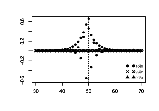
Figure 3: Plot of $\{u_{i}(B_{n})\}$ for $i=1,2,3$ (left) and $i=998,999,1000$ (right) around the break point ($k=50$, vertical dashed line) under a single SCM. Here $n=1,000$ and $(\rho,\rho+\epsilon)$ = (0.3, 0.5).

Noting that, if $A_{0,n}$ corresponds to the precision matrix of the null model in (1.5), then,

$$[u_{i}(A_{0,n})]_{j}=O(n^{-1/2})\qquad 1\leq i,j\leq n.$$

However, under the alternative of the single SCM, Figure 3 illustrates that $u_{1}(B_{n})$ and $u_{1000}(B_{n})$ has unexpectedly large values near the break point $k=50$. That is

$$[u_{i}(B_{n})]_{k}=O(1)\qquad i=1,1000$$

and the adjacent eigenvectors ($u_{2}(B_{n})$,$u_{3}(B_{n})$, $u_{998}(B_{n})$, and $u_{999}(B_{n})$) take value of an order of $n^{-1/2}$ at $k$-th element. We believe that using a similar technique as in Benaych-Georges and Nadakuditi (2011), Theorem 2.3, it is possible to show

$$\left|u_{i}(B_{n})\right|_{\infty}=\left\{\begin{array}[]{ll}O(1)&i=1,n\\ O(n^{-1/2})&i\neq 1,n\\ \end{array}\right.$$

where $\left|u_{i}(B_{n})\right|_{\infty}=\max_{1\leq j\leq n}\left|[u_{i}(B_{n})\right|$ and

$$arg\,max_{1\leq i\leq n}\left|[u_{1}(B_{n})]_{i}\right|=k\qquad arg\,max_{1\leq i\leq n}\left|[u_{n}(B_{n})]_{i}\right|=k-1.$$

Therefore, if above conjectures are true, then we can identify the break point $k$ by finding the index that takes the maximum value in $u_{1}(B_{n})$. We leave this to future research.

5 Outlier detection of a panel time series

In this section, we apply the results from Section 3 to detect outliers of a panel time series. Consider the panel autoregressive model

$$y_{j,t}=\rho_{t}y_{j,t-1}+z_{j,t}\qquad t\geq 0,1\leq j\leq B$$ (5.1)

where $\{z_{jt}\}$ are $i.i.d.$ random variables with mean zero and variance 1, $\{\rho_{t}\}$ are common AR coefficients across $j$ that satisfy the SCM in (1.2).

Let $\underline{y}_{j;n}=(y_{j,1},...,y_{j,n})^{\top}$, be the $j$th observation with common variance $var(\underline{y}_{j;n})=\Sigma_{n}$ and $\Omega_{n}=(\Sigma_{n})^{-1}$ be its inverse. Then, our goal is to find a consistent estimator of $out(\{\Omega_{n}\})$. To do so, we need obtain a consistent estimator of $\Omega_{n}$. A natural plug-in estimator for $\Sigma_{n}$ is $\widehat{\Sigma}_{n,B}=B^{-1}\sum_{j=1}^{B}(\underline{y}_{j;n}-\overline{y}_{j}\textbf{1}_{n})(\underline{y}_{j;n}-\overline{y}_{j}\textbf{1}_{n})^{\top}$, where $\overline{y}_{j}=n^{-1}\sum_{t=1}^{n}y_{j,t}$ and $\textbf{1}_{n}$ is a vector of ones. Then, we may $\widehat{\Omega}_{n,B}=(\widehat{\Sigma}_{n,B})^{-1}$ as our estimator. $\widehat{\Omega}_{n,B}$ is consistent when $n$ is fixed and $B\rightarrow\infty$. However, if $n$ increases at the same rate as $B$, i.e., $\lim B/n=\tau\in(0,\infty)$, $\widehat{\Omega}_{n,B}$ is no longer a consistent estimator of $\Omega_{n}$ (See, e.g., Wu and Pourahmadi (2009)). However, from Lemma 2.1, $\Omega_{n}$ is a tri-diagonal matrix, thus it is sparse. Therefore, we implement an estimator from Cai et al. (2011), using a constrained $\ell_{1}$ minimization method. In detail, let $\widetilde{\Omega}_{1}$ be the solution of the following minimization problem

$$\min\left|\Omega\right|_{1}\quad\text{subject to:}\quad\left|\widehat{\Sigma}_{n,B}\Omega-I_{n}\right|_{\infty}\leq\lambda_{n},$$

where for $A=(a_{ij})$, $\left|A\right|_{1}=\sum_{i,j=1}^{n}|a_{ij}|$ and $\left|A\right|_{\infty}=\max_{1\leq i,j\leq n}|a_{ij}|$, $\widehat{\Sigma}_{n,B}$ is a plug-in estimator, and $\lambda_{n}$ is a tuning parameter. and define $\widetilde{\Omega}_{n,B}$ as a symmetrization of $\widetilde{\Omega}_{1}$

$$[\widetilde{\Omega}_{n,B}]_{i,j}=[\widetilde{\Omega}_{1}]_{i,j}\wedge[\widetilde{\Omega}_{1}]_{j,i}.$$ (5.2)

We require the following assumptions on the tail behavior of $y_{j,t}$.

Assumption 5.1

$\underline{y}_{1;n}$ satisfies the exponential-type tail condition as described in Cai et al. (2011), i.e., there exist $0<\eta<1/4$ and $K>0$ such that $(\log n)/B\leq\eta$ and

$$\max_{1\leq i\leq N}\mathbb{E}\exp{(ty_{1,i}^{2})}\leq K<\infty\quad\forall|t|\leq\eta,$$

Note that if the innovations $\{\varepsilon_{jt}\}$ are Gaussian, then Assumption 5.1(i) is satisfied.

The following lemma gives a concentration inequality between $\widetilde{\Omega}_{n,B}$ and $\Omega_{n}$.

Lemma 5.1

Let $\{y_{j,t}\}$ be a panel time series with recursion (5.1) where AR coefficients satisfy the SCM in (1.2). Suppose that Assumption 5.1 holds. Let $\Omega_{n}$ be the true precision matrix and $\widetilde{\Omega}_{n,B}$ is an estimator as defined in (5.2). Then, for all $\tau>0$, there exist a constant $C_{\tau}>0$ such that

$$P\left(\max_{1\leq i\leq n}|\lambda_{i}(\widetilde{\Omega}_{n,B})-\lambda_{i}(\Omega_{n})|\leq C_{\tau}\sqrt{\frac{\log n}{B}}\right)\geq 1-4n^{-\tau}.$$

PROOF. See Appendix C. $\Box$

By this lemma, if $(\log n)/B\rightarrow 0$ as $n,B\rightarrow\infty$, $\widetilde{\Omega}_{n,B}$ is positive definite and a consistent estimator for $\Omega_{n}$ with a high probability.

Next, we estimate $out(\{\Omega_{n}\})$ using $\widetilde{\Omega}_{n,B}$. To do so, let $\widehat{\rho}_{n}$ be the consistent estimator of the original AR coefficient $\rho$. The Yule-Walker estimator is one example of $\widehat{\rho}_{n}$. Let

$$\widehat{out}(\widetilde{\Omega}_{n,B})=spec(\widetilde{\Omega}_{n,B})\cap[a_{\widehat{\rho}_{n}},b_{\widehat{\rho}_{n}}]^{c}$$ (5.3)

where $a_{\widehat{\rho}_{n}}$ and $b_{\widehat{\rho}_{n}}$ are defined as in (2.8). To show the consistency of the set of outliers, we require an appropriate distance measure of sets. For sets $X$ and $Y$, we define the Hausdorff distance of $X$ and $Y$

$$d_{H}(X,Y)=\max\{\sup_{x\in X}\inf_{y\in Y}|x-y|,\sup_{y\in Y}\inf_{x\in X}|x-y|\}.$$

The follow theorem gives a consistent result of an outlier estimator.

Theorem 5.1

Assume the same set of notation and assumption as in Lemma 5.1 hold. Let $\widehat{\rho}_{n}$ be the consistent estimator of the original AR coefficient $\rho$ and $\widehat{out}(\widetilde{\Omega}_{n,B})$ as defined in (5.3). Then,

$$d_{H}\left(\widehat{out}(\widetilde{\Omega}_{n,B}),out(\{\Omega_{n}\})\right)\stackrel{{\scriptstyle P}}{{\rightarrow}}0$$ (5.4)

as $n,B\rightarrow\infty$, and $(\log n)/B\rightarrow 0$.

PROOF. See Appendix C. $\Box$

6 Simulations

To substantiate the proposed methods, we conduct some simulations. We assume the single SCM with the length of the time series $n=100$ and the break point at $k=50$. An original AR coefficient varies $\rho=0.1,0.3,0.5,0.7,$ and $0.9$ and to see the relative effect of the magnitude of change, we use three different ratios $\varepsilon/\rho=0.5,1,2$ for each $\rho$. Moreover, to see the asymptotic effect of the number of panels, we use $B=100,500,1000,5000$ for each parameter set $(\rho,\varepsilon)$.

For a given $(\rho,\varepsilon,B)$, we generate $\{y_{j,t}\}$ as in (5.1) where $\{\varepsilon_{j,t}\}$ are i.i.d. standard normal. Let $\Omega_{n}$ be the true precision matrix and $\widetilde{\Omega}_{n,B}$ is an estimator as defined in (5.2). By Theorem 3.2, $out(\{\Omega_{n}\})=\{\lambda_{L},\lambda_{R}\}$ which are explicit formulas for the two outliers $\lambda_{L}(=m)<a_{\rho}$ and $\lambda_{R}(=M)>b_{\rho}$ that are given in the theorem. Since we know there are exactly two outliers, we use

$$\widehat{out}(\widetilde{\Omega}_{n,B})=\{\widehat{\lambda}_{L},\widehat{\lambda}_{R}\}$$

where $\widehat{\lambda}_{L}=\lambda_{1}(\widetilde{\Omega}_{n,B})$ and $\widehat{\lambda}_{R}=\lambda_{n}(\widetilde{\Omega}_{n,B})$ as an estimator of outliers.

All simulations are conducted in 1000 replications and obtain the value $(\widehat{\lambda}_{L,i},\widehat{\lambda}_{R,i})$ for $i=1,...,1000$. For each simulation, we calculate the mean absolute error (which is an equivalent norm of the Hausdorff norm)

$$\text{MAE}_{i}=\frac{1}{2}\left(|\widehat{\lambda}_{L,i}-\lambda_{L}|+|\widehat{\lambda}_{R,i}-\lambda_{R}|\right)\qquad 1\leq i\leq 1000.$$ (6.1)

Table 1 shows the average and standard deviation (in parentheses) of the mean absolute error.

$\rho$	$\varepsilon/\rho$	$B$
		100	500	1000	5000
0.1	0.5	0.15(0.03)	0.05(0.02)	0.03(0.01)	0.01(0.00)
	1	0.13(0.03)	0.05(0.02)	0.03(0.01)	0.01(0.01)
	2	0.10(0.03)	0.03(0.02)	0.03(0.01)	0.01(0.01)
0.3	0.5	0.09(0.05)	0.04(0.02)	0.02(0.01)	0.02(0.01)
	1	0.13(0.04)	0.04(0.02)	0.04(0.02)	0.02(0.01)
	2	0.22(0.08)	0.08(0.04)	0.06(0.04)	0.04(0.02)
0.5	0.5	0.20(0.08)	0.07(0.04)	0.07(0.03)	0.04(0.02)
	1	0.23(0.10)	0.12(0.07)	0.10(0.05)	0.06(0.03)
	2	0.39(0.19)	0.21(0.11)	0.17(0.09)	0.09(0.04)
0.7	0.5	0.28(0.15)	0.08(0.04)	0.04(0.02)	0.03(0.02)
	1	0.39(0.20)	0.09(0.05)	0.07(0.05)	0.05(0.03)
	2	0.67(0.31)	0.17(0.10)	0.15(0.10)	0.10(0.06)
0.9	0.5	0.48(0.22)	0.13(0.07)	0.07(0.05)	0.04(0.03)
	1	0.55(0.29)	0.14(0.08)	0.09(0.07)	0.05(0.04)
	2	0.54(0.33)	0.26(0.18)	0.18(0.12)	0.07(0.06)

Table 1: Average and standard deviation (in parentheses) of the mean absolute error as defined in (6.1) for each $(\rho,\varepsilon,B)$. The true model is the single SCM with the length of time series $n=100$ and break point $k=50$.

For all simulations, as $B$ goes to $\infty$, error decreases and goes to zero. Note that when $n$ is fixed and $B$ goes to $\infty$, $\widehat{\lambda}_{L}$ and $\widehat{\lambda}_{R}$ estimates $\lambda_{1}(\Omega_{n})$ and $\lambda_{n}(\Omega_{n})$, respectively, which is not exactly the “ideal” outliers $out(\{\Omega_{n}\})$. Thus, there are two sources of bias due to the finite $n$ and $k$. However, at least for the range of parameters that we studied in this section, the bias due to the finite $n$ and $k$ is negligible for $\rho=0.1$ and $0.3$, and reasonable small for the larger $\rho$.

An error increases when $\rho$ increases. A relatively weak performance of the estimator for the large $\rho$ value could be due to the break point. By Remark 3.1(iii), the bias due to the finite $k$ is an order of $O(|c|^{k})$ for some $<|c|<1$. The constant $c$ depends on the value $\rho$ and is close to one when $|\rho|$ is close to the boundary, leading to a larger $O(|c|^{k})$. However, the effect of ratio $\varepsilon/\rho$ is not coherent. For $\rho=0.3,0.5,0.7$, and $0.9$, the bias tends to increase when $\varepsilon/\rho$ increases. Whereas, when $\rho=0.1$, it is the opposite.

7 Discussion on the heteroscedasticity model

Our method can also be applied to the heteroscedasticity model. Consider the heteroscedasticity autoregressive model

$$\widetilde{y}_{t}=\rho\widetilde{y}_{t-1}+\sigma_{t}\widetilde{z}_{t}\qquad t\geq 1$$

where $\rho\in(-1,1)/\{0\}$ and $\{\widetilde{z}_{t}\}$, a white noise process with unit variance. We assume the error variances have the following structure

$$\sigma_{t}^{2}=\sigma^{2}+\sum_{j=1}^{m}\xi_{j}I_{E_{j}}(t)\qquad t\geq 1.$$ (7.1)

where $\{E_{j}\}_{j=1}^{m}$ are disjoint intervals and $\xi_{j}>-\sigma^{2}$ is the nonzero constant. Let $C_{n}$ be a precision matrix of $\widetilde{\underline{y}}_{n}=(\widetilde{y}_{1},...,\widetilde{y}_{n})^{\prime}$. Then, analogous to Lemma 2.1 and Theorem 2.1, we can show (without proofs)

$$C_{n}]_{i,j}=\begin{cases}\sigma_{n}^{2}&i=j=n\\ \sigma_{i}^{2}+\sigma_{i+1}^{2}\rho_{i+1}^{2}&i=j<n\\ -\sigma_{i\vee j}^{2}\rho_{i\vee j}&|i-j|=1\\ 0&o.w.\end{cases}.$$

and if $\max_{j}|E_{j}|/n\rightarrow 0$ as $n\rightarrow\infty$, then

$$\mu_{C_{n}}\stackrel{{\scriptstyle\mathcal{D}}}{{\rightarrow}}\sigma^{2}\mu_{\rho}.$$ (7.2)

With loss of the generality, we set $\sigma^{2}=1$. From (7.2), the null ($m=0$ in (7.1)) and alternative of heteroscedasticity model have the same ASD, $\mu_{\rho}$. It is natural to think whether we can observe outlier(s) in the alternative model.

Figure 4 shows the histogram of ESD of $C_{n}$ ($n=1000$) where

$$\sigma_{t}^{2}=1+\xi I_{\{50\}}(t)\qquad 1\leq t\leq 1000$$

for two different $\xi$ values ( $\xi=0.3$ (left) and $\xi=-0.3$ (right)). Note that histogram of ESD under null is the left panel of Figure 2).

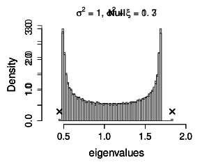
Figure 4: ESD of the precision matrix of $C_{n}$ for different $\xi$ values. Here $n=1,000$, $\rho=0.3$, $\sigma^{2}=1$, $m=1$, $k=50$, and $h=1$. $\sigma^{2}+\xi$ = 1.3 (left) and 0.7 (right). Crosses indicate outliers.

Unlike the change in the coefficient model, behavior of an outlier is different in the heteroscedasticity model. First, we only observe a single (right) outlier when $\sigma^{2}+\xi>\sigma^{2}$ (in the single SCM, we observe two outliers when $|\rho+\varepsilon|>|\rho|$). Next, even though $\sigma^{2}+\xi<\sigma^{2}$, we are able to observe an (left) outlier (there is no outlier when $|\rho+\varepsilon|<|\rho|$ in the single SCM). We can further investigate the behavior of $out(\{C_{n}\})$ using similar techniques in Section 3, but this remains an avenue for future research.

Summary of results in the Appendix

To navigate the Appendix, we briefly summarize the contents of each section.

• In Appendix A, we list some properties of the common ASD, $\mu_{\rho}$, of the null and alternative model defined in Section 2.2. Specifically, we give an explicit formula for the Stieltjes transform of $\mu_{\rho}$ and the moments of $\mu_{\rho}$. These properties are not directly used in the main paper, but they may also be of independent interest. Moreover, these properties are frequently used in the proofs of Section 3.

• In Appendix B, we give prove technical lemmas required in the proof of Theorems in Sections 2 and 3.

• In Appendix C, we give a proofs in the main paper. Proof of Theorem 3.2 involves 7 steps and quite technical. [Step4]–[Step7] can be skipped on first reading. Proof of Theorem 3.3 may gives more insights on the proof techniques.

Appendix A Properties of $\mu_{\rho}$

For a probability measure $\mu$ on the real line, we define the Stieltjes transform (or the Cauchy transform) of $\mu$ as

$$G_{\mu}(z)=\int_{supp(\mu)}~{}\frac{1}{z-x}d\mu(x),\qquad z\in\mathbb{R}\backslash supp(\mu)$$

where $supp(\mu)$ is a support of $\mu$. The Stieltjes transform plays an important tool in Random Matrix literatures (see Tao (2012), Section 2.4.3. and the references therein). Moreover, under certain regularity conditions, it is related to the moments of the measure via

$$G_{\mu}(z)=\sum_{k=0}^{\infty}\frac{m_{k}(\mu)}{z^{k}}.$$ (A.1)

where $m_{k}(\mu)=\int x^{k}d\mu(x)$ is the $k$th moment of $\mu$. Given the measure $\mu$, it is unwieldy to get an explicit form of the Stieltjes transform of $\mu$. However, within our framework, we have a simple analytic form for $G_{\mu_{\rho}}$.

Proposition A.1

Let $\mu_{\rho}$ is defined as in Lemma 2.2. Further, let $a_{\rho}$ and $b_{\rho}$ defined as in (2.8) are the lower and upper bound of the support of $\mu_{\rho}$ respectively. Then, for any $z\in(-\infty,a_{\rho})\cup(b_{\rho},\infty)$, the Stieltjes transform of $\mu_{\rho}$ at $z$ is

$$G_{\mu_{\rho}}(z)=\left\{\begin{array}[]{ll}\frac{1}{\sqrt{(z-a_{\rho})(z-b_{\rho})}}&z>b_{\rho}\\ -\frac{1}{\sqrt{(z-a_{\rho})(z-b_{\rho})}}&z<a_{\rho}\\ \end{array}\right..$$

PROOF. See Appendix C. $\Box$

The following corollary gives an expression of the moments of $\mu_{\rho}$.

Corollary A.1

The $k^{th}$ moment of $\mu_{\rho}$ is

$$m_{k}(\mu_{\rho})=\frac{1}{2\pi}\int_{0}^{2\pi}(1+\rho^{2}-2\rho\cos x)^{k}dx$$

PROOF. See Appendix C. $\Box$

Remark A.1

Corollary A.1 can be generalized to AR$(p)$ process with the following recursion

$$Y_{t}=\sum_{j=1}^{p}\phi_{j}Y_{t-j}+Z_{t}\qquad t\in\mathbb{Z},$$

where the roots of the characteristic polynomial $\phi(z)=1-\sum_{j=1}^{p}\phi_{j}z^{j}$ lies outisde of the unit circle. Define $\mu_{\underline{\phi}}$ be the ESD of an inverse matrix $\underline{Y}_{n}=(Y_{1},...,Y_{n})$, where $\underline{\phi}=(\phi_{1},...,\phi_{p})^{\prime}$. Then it is easy to show

$$m_{k}(\mu_{\underline{\phi}})=\frac{1}{2\pi}\int_{0}^{2\pi}\big{|}\phi(e^{-ix})\big{|}^{2k}dx,\qquad k=0,1,....$$

Appendix B Technical Lemma

Lemma B.1

Let $|a|>1$ be a constant and

$$z_{1}=-a-\sqrt{a^{2}-1}\qquad z_{2}=-a+\sqrt{a^{2}-1}.$$

Then, for any positive integer $k_{1}$ and $k_{2}$, we have the following explicit form of the integration.

$$\frac{1}{2}G(k_{1},k_{2}):=\frac{1}{2\pi}\int_{0}^{2\pi}\frac{\sin(k_{1}x)\sin(k_{2}x)}{a+\cos x}dx=\left\{\begin{array}[]{ll}\frac{1}{z_{2}-z_{1}}\big{(}z_{2}^{|k_{1}-k_{2}|}-z_{2}^{k_{1}+k_{2}}\big{)}&a>1\\ \frac{1}{z_{1}-z_{2}}\big{(}z_{1}^{|k_{1}-k_{2}|}-z_{1}^{k_{1}+k_{2}}\big{)}&a<-1\end{array}\right..$$ (B.1)

Therefore, we can approximate

$$G(k,k+h)=\frac{a}{|a|}\frac{1}{\sqrt{a^{2}-1}}z_{1}^{h}(\text{or }z_{2}^{h})+O\left(|z_{1}|^{k}\wedge|z_{2}^{k}|\right)\approx\frac{a}{|a|}\frac{1}{\sqrt{a^{2}-1}}z_{1}^{h}(\text{or }z_{2}^{h}).$$

Moreover for large $h$, $G(k,k+h)\approx 0$.

PROOF. We will prove for $a>1$, and $a<-1$ is similar. Parametrize $z=e^{ix}$ where $i=\sqrt{-1}$. Then,

$$dz=izdx,\qquad\cos x=\frac{1}{2}(z+z^{-1}),\qquad\text{and}\qquad\sin kx=\frac{1}{2i}(z^{k}-z^{-k}).$$

Let $C$ be a counterclockwise contour of unit circle on the complex field starts from 1, and $\oint_{C}$ denote a cylclic interal along with contour $C$. Then,

$$\frac{1}{2\pi}\int_{0}^{2\pi}\frac{\sin(k_{1}x)\sin(k_{2}x)}{a+\cos x}dx = \frac{1}{2\pi}\oint_{C}\left(\frac{-\frac{1}{4}(z^{k_{1}}-z^{-k_{1}})(z^{k_{2}}-z^{-k_{2}})}{\frac{1}{2}(z+z^{-1})+a}\right)\frac{dz}{iz}$$

$$= -\frac{1}{2}\frac{1}{2\pi i}\oint_{C}\frac{(z^{k_{1}}-z^{-k_{1}})(z^{k_{2}}-z^{-k_{2}})}{(z^{2}+2az+1)}dz$$

$$= -\frac{1}{2}\frac{1}{2\pi i}\oint_{C}\frac{(z^{2k_{1}}-1)(z^{2k_{2}}-1)}{z^{k_{1}+k_{2}}(z-z_{1})(z-z_{2})}dz.$$

Since $a>1$, we have $|z_{2}|<1<|z_{1}|$, thus the poles of $\frac{(z^{2k_{1}}-1)(z^{2k_{2}}-1)}{z^{k_{1}+k_{2}}(z-z_{1})(z-z_{2})}$ in the interior of $C$ is $z_{2}$ with mutiplicity 1, and $0$ with multiplicity $(k_{1}+k_{2})$. Therefore by Cauchy’s integral formula,

$$\frac{1}{2\pi i}\oint_{C}\frac{(z^{2k_{1}}-1)(z^{2k_{2}}-1)}{z^{k_{1}+k_{2}}(z-z_{1})(z-z_{2})}dz = \text{Res}\left(\frac{(z^{2k_{1}}-1)(z^{2k_{2}}-1)}{z^{k_{1}+k_{2}}(z-z_{1})(z-z_{2})},z_{2}\right)+\frac{1}{(k_{1}+k_{2}-1)!}f^{(k_{1}+k_{2}-1)}(0)$$

$$= \frac{(z_{2}^{k_{1}}-z_{1}^{k_{1}})(z_{2}^{k_{2}}-z_{1}^{k_{2}})}{z_{2}-z_{1}}+\frac{1}{(k_{1}+k_{2}-1)!}f^{(k_{1}+k_{2}-1)}(0),$$

where Res is a Residue, $f(z)=\frac{(z^{2k_{1}}-1)(z^{2k_{2}}-1)}{(z-z_{1})(z-z_{2})}$, $f^{(n)}$ be the $n$th derivative of $f$. For the second equality, we use $z_{2}^{-1}=z_{1}$. Next, observe that $\big{|}\frac{z}{z_{1}}\big{|},~{}\big{|}\frac{z}{z_{2}}\big{|}<1$ for $z$ near the origin, thus we have the following Taylor expansion of $f$ at $z=0$

$$f(z) = \frac{(z^{2k_{1}}-1)(z^{2k_{2}}-1)}{(z-z_{1})(z-z_{2})}$$ (B.2)

$$= \frac{1}{z_{2}-z_{1}}\left(z^{2(k_{1}+k_{2})}-z^{2k_{1}}-z^{2k_{2}}+1\right)\left[\frac{1}{z_{1}}\left(\frac{1}{1-z/z_{1}}\right)-\frac{1}{z_{2}}\left(\frac{1}{1-z/z_{2}}\right)\right]$$

$$= \frac{1}{z_{2}-z_{1}}\left(z^{2(k_{1}+k_{2})}-z^{2k_{1}}-z^{2k_{2}}+1\right)\left[\frac{1}{z_{1}}\sum_{j=0}^{\infty}\left(\frac{z}{z_{1}}\right)^{j}-\frac{1}{z_{2}}\sum_{j=0}^{\infty}\left(\frac{z}{z_{2}}\right)^{j}\right].$$

With loss of generality, assume $k_{1}\leq k_{2}$. Noting that $\frac{1}{(k_{1}+k_{2}-1)!}f^{(k_{1}+k_{2}-1)}(0)$ is the coefficient of $z^{k_{1}+k_{2}-1}$ of the power series expension of $f(z)$ at $z=0$, we have the following two cases.

case 1: $k_{1}=k_{2}=k$.

In this case, $1\leq k_{1}+k_{2}-1<\{2(k_{1}+k_{2}),2k_{1},2k_{2}\}$, thus the coefficient of $z^{k_{1}+k_{2}-1}$ in (B.2) is

$$\frac{1}{(k_{1}+k_{2}-1)!}f^{(k_{1}+k_{2}-1)}(0)=\frac{1}{z_{2}-z_{1}}\left(z_{1}^{-2k}-z_{2}^{-2k}\right)=\frac{1}{z_{2}-z_{1}}(z_{2}^{2k}-z_{1}^{2k}).$$

Therefore,

$$\frac{1}{2\pi}\int_{0}^{2\pi}\frac{\sin(k_{1}x)\sin(k_{2}x)}{a+\cos x}dx = -\frac{1}{2}\frac{1}{2\pi i}\oint_{C}\frac{(z^{2k_{1}}-1)(z^{2k_{2}}-1)}{z^{k_{1}+k_{2}}(z-z_{1})(z-z_{2})}dz$$

$$= -\frac{1}{2}\frac{1}{(z_{2}-z_{1})}\big{[}(z_{2}^{k}-z_{1}^{k})^{2}+(z_{2}^{2k}-z_{1}^{2k})\big{]}=\frac{1}{z_{2}-z_{1}}\left(1-z_{2}^{2k}\right).$$

case 1: $k_{1}<k_{2}$.

In this case, $\{1,2k_{1}\}\leq k_{1}+k_{2}-1<\{2(k_{1}+k_{2}),2k_{2}\}$, thus the coefficient of $z^{k_{1}+k_{2}-1}$ in (B.2) is

$$\frac{1}{(k_{1}+k_{2}-1)!}f^{(k_{1}+k_{2}-1)}(0) = \frac{1}{z_{2}-z_{1}}\left(z_{1}^{-(k_{1}+k_{2})}-z_{1}^{-(k_{2}-k_{1})}-z_{2}^{-(k_{1}+k_{2})}+z_{2}^{-(k_{2}-k_{1})}\right)$$

$$= \frac{1}{z_{2}-z_{1}}(z_{2}^{k_{1}+k_{2}}-z_{1}^{k_{1}}z_{2}^{k_{2}}-z_{1}^{k_{1}+k_{2}}+z_{1}^{k_{2}}z_{2}^{k_{1}}).$$

Therefore,

$$\frac{1}{2\pi}\int_{0}^{2\pi}\frac{\sin(k_{1}x)\sin(k_{2}x)}{a+\cos x}dx = -\frac{1}{2}\frac{1}{(z_{2}-z_{1})}\bigg{[}(z_{2}^{k_{1}}-z_{1}^{k_{1}})(z_{2}^{k_{2}}-z_{1}^{k_{2}})+$$

$$(z_{2}^{k_{1}+k_{2}}-z_{1}^{k_{1}}z_{2}^{k_{2}}-z_{1}^{k_{1}+k_{2}}+z_{1}^{k_{2}}z_{2}^{k_{1}})\bigg{]}$$

$$= \frac{1}{z_{2}-z_{1}}\left(z_{2}^{k_{2}-k_{1}}-z_{2}^{k_{1}+k_{2}}\right).$$

In both cases,

$$\frac{1}{2\pi}\int_{0}^{2\pi}\frac{\sin(k_{1}x)\sin(k_{2}x)}{a+\cos x}dx=\frac{1}{z_{2}-z_{1}}\left(z_{2}^{|k_{1}-k_{2}|}-z_{2}^{k_{1}+k_{2}}\right).$$

Thus proves the lemma. $\Box$

Lemma B.2 (Chebyshev polynomials)

Let

$$U_{0}(x)=1\qquad U_{n}(x)=\det\begin{pmatrix}2x&1&&0\\ 1&\ddots&\ddots\\ &\ddots&2x&1\\ 0&&1&2x\end{pmatrix}\quad n\geq 1$$ (B.3)

be the Chebyshev polynomial of the second kind of order $n$. Then,

$$U_{n}(x)=2xU_{n-1}(x)-U_{n-2}(x)$$ (B.4)

$$U_{n}(x)=2^{n}\prod_{k=1}^{n}\left(x-\cos\left(\frac{k\pi}{n+1}\right)\right)$$ (B.5)

$$\text{Zeros of }U_{n}\text{ and }U_{n+1}\text{ are interacing.}$$ (B.6)

PROOF. Proofs are elementary. See Rivlin (2020) for details. $\Box$

Lemma B.3

Define the matrix valued function $\Delta_{n}(x)$

$$\Delta_{n}(x)=\begin{pmatrix}2x+f(x)&1&&&0\\ 1&2x&1&&\\ &\ddots&\ddots&\ddots\\ &&1&2x&1\\ 0&&&1&2x+g(x)\end{pmatrix}\in\mathbb{R}^{n\times n}.$$ (B.7)

Then, for $n\geq 2$,

$$\det\Delta_{n}(x)=\big{(}2x+f(x)+g(x)\big{)}U_{n-1}(x)+\big{(}f(x)g(x)-1\big{)}U_{n-2}(x),$$

where $U_{n}$ is defined as in (B.3).

PROOF. Define $\widetilde{\Delta}_{n}(x)$ by

$$\widetilde{\Delta}_{n}(x)=\begin{pmatrix}2x+f(x)&1&&0\\ 1&\ddots&\ddots\\ &\ddots&2x&1\\ 0&&1&2x\end{pmatrix}\in\mathbb{R}^{n\times n}.$$

Then, using the definition of $U_{n}$ by directly calculating the determinant, it is easy to show

$$\det\widetilde{\Delta}_{n}(x)=(2x+f(x))U_{n-1}(x)-U_{n-2}(x)=U_{n}(x)+f(x)U_{n-1}(x).$$ (B.8)

The last identity is due to (B.4).

Using similar argument for $\Delta_{n}(x)$ combining with (B.8), we get

$$\det\Delta_{n}(x) = (2x+g(x))\widetilde{\Delta}_{n-1}(x)-\widetilde{\Delta}_{n-2}(x)$$

$$= \left(2x+g(x)\right)\left(U_{n-1}(x)+f(x)U_{n-2}(x)\right)-\left(U_{n-2}(x)+f(x)U_{n-3}(x)\right)$$

$$= \left(2x+g(x)\right)U_{n-1}(x)+\left(2xf(x)+f(x)g(x)-1\right)U_{n-2}(x)-f(x)U_{n-3}(x)$$

$$= \left(2x+g(x)+f(x)\right)U_{n-1}(x)+\left(f(x)g(x)-1\right)U_{n-2}(x).$$

Thus proves the lemma. $\Box$

Lemma B.4 (Weyl inequalities)

For $n\times n$ Hermitian matrices $A_{n},B_{n},\text{and }X_{n}$ with $A_{n}=B_{n}+X_{n}$, define $\mu_{1}\geq...\geq\mu_{n}$, $\nu_{1}\geq...\geq\nu_{n}$, and $\xi_{1}\geq...\geq\xi_{n}$ the eigenvalues of $A_{n}$, $B_{n}$, and $X_{n}$ respectively. Then, for all $j+k-n\geq i\geq r+s-1$,

$$\nu_{j}+\xi_{k}\leq\mu_{i}\leq\nu_{r}+\xi_{s}.$$

Lemma B.5

A compactly supported probability measure on $\mathbb{R}$ is uniquely determined by its moments.

PROOF. Let $\mu$ be a compactly supported probability on the real line with support is in an interval $[a,b]$. It is obvious that $\mu$ has all moments, denote $\{m_{k}\}_{k=0}^{\infty}$, and $|m_{k}|\leq(|a|\vee|b|)^{k}$. Then, the power series $\sum_{k\geq 0}m_{k}r^{k}/k!$ converges for every $r\in\mathbb{R}$, thus by Billingsley (2008),Theorem 30.1, $\mu$ is uniquely determined. $\Box$

Lemma B.6

Let $A,B$ are $n\times n$ Hermitian matrices. Then,

$$\max_{1\leq i\leq n}|\lambda_{i}(A)-\lambda_{i}(B)|\leq||A-B||_{2}$$

where $||A||_{2}=\sqrt{\lambda_{n}(AA^{*})}$ is a spectral norm.

PROOF. We start with the Courant-Fischer min-max theorem, i.e., Let $A$ be an $n\times n$ Hermitian with eigenvalues $\lambda_{1}\geq...\geq\lambda_{n}$. Then,

$$\lambda_{i}=\sup_{dim(V)=i}\inf_{v\in V,|v|=1}v^{*}Av.$$

For any given subspace $V$ with $dim(V)=i$ and for all $v\in V$ with $|v|=1$,

$$v^{*}(A+B)v=v^{*}Av+v^{*}Bv\leq v^{*}Av+||B||_{2}.$$

Take $\sup_{dim(V)=i}\inf_{v\in V,|v|=1}$ on both side gives $\lambda_{i}(A+B)\leq\lambda_{i}(A)+||B||_{2}$, and plug in $A\leftarrow A+B$ and $B\leftarrow(-B)$ gives $\lambda_{i}(A)\leq\lambda_{i}(A+B)+||B||_{2}$. Therefore, for all $i$,

$$|\lambda_{i}(A+B)-\lambda_{i}(A)|\leq||B||_{2}$$

and thus take $\max$ and plug in $B\leftarrow B-A$ gives a desired inequality. $\Box$

Appendix C Proofs

This section contains proofs in the main paper. Most of the case, we only give a prove for the case when $\rho>0$, i.e., the original AR coefficient is positive. Proof for $\rho<0$ is similar.

Proof of Lemma 2.1

Let $\underline{z}_{n}=(z_{1},...,z_{n})^{\prime}$. Then, $var(\underline{z}_{n})=I_{n}$, where $I_{n}$ is an identity matrix of order $n$. Using the recursive formula in (1.1), it is easy to obtain the following linear equation

$$\underline{z}_{n}=L_{n}\underline{y}_{n}\qquad\text{where}\qquad L_{n}=\begin{pmatrix}1&0&\cdots&0\\ -\rho_{2}&1&\cdots&0\\ \vdots&\ddots&\ddots&0\\ 0&0&-\rho_{n}&1\end{pmatrix}\in\mathbb{R}^{n\times n}.$$

Take the variance on each side above and by simple algebra we get $A_{n}=[var(\underline{y}_{n})]^{-1}=L_{n}^{\top}[var(\underline{z}_{n})]^{-1}L_{n}$ and deduce (2.2). $\square$

Proof of Theorem 2.1

We give a proof when $m=1$, and the generalization to $m\geq 2$ is straightforward. Let $A_{0,n}$ and $B_{n}$ be the precision matrices under the null (i.e. $m=0$ in (1.2)) and alternative respectively. By Szegö’s limit theorem (See Section 2), it is easy to show that $\mu_{A_{0,n}}$ converges weakly to some measure, denote, $\mu_{\rho}$. By the Gershgorin circle theorem, $\lambda_{n}(A_{0,n})<4$, thus $\mu_{\rho}$ is compactly supported. We will first show (2.9) for $h=1$, and extend to $h\geq 2$.

case 1: $h=1$. Suppose that we have shown the following

$$\lim_{n\rightarrow\infty}\frac{1}{n}tr(B_{n}^{j})=\lim_{n\rightarrow\infty}\frac{1}{n}tr(A_{0,n}^{j})=m_{j}(\mu_{\rho})\qquad j\geq 0.$$ (C.1)

where $m_{j}(\mu_{\rho})$ is the $j$th moment of $\mu_{\rho}$. Then, $j$th moment of $\mu_{B_{n}}$ (which is equal to $n^{-1}tr(B_{n}^{j})$) converges to the $j$th moment of $\mu_{\rho}$. Therefore, by Lemma B.5 and Billingsley (2008), Theorem 30.2, we get $\mu_{B_{n}}\stackrel{{\scriptstyle\mathcal{D}}}{{\rightarrow}}\mu_{\rho}$ as desired. Therefore, it is enough to show (C.1).

Let $R_{n}=B_{n}-A_{0,n}$. Then, from (2.2), $R_{n}$ is a matrix entries are 0 except for $2\times 2$ submatrix. By the linearity

$$tr(B_{n}^{j})=tr\left((A_{0,n}+R_{n})^{j}\right)=\sum_{\alpha_{i}\in\{\circ,~{}\ast\}}tr\big{(}X_{n}^{(\alpha_{1})}\cdots X_{n}^{(\alpha_{j})}\big{)}$$ (C.2)

Where $X_{n}^{(\alpha)}=\left\{\begin{array}[]{ll}A_{0,n}&\alpha=\circ\\ R_{n}&\alpha=\ast\end{array}\right.$. Observe that $R_{n}$ has nonzero elements on $[R_{n}]_{i,j}$ for $(i,j)=(k-1,k-1),(k-1,k),(k,k-1)$ where $k$ is the break point. Thus, for any matrix $X\in\mathbb{R}^{n\times n}$, $[XR_{n}]_{\ell,m}=0$ unless $\ell=k-1,k$. That is, every column of $XR_{n}$ are zero except the $(k-1)$th and $k$th columns. Next, by the commutative of the trace function, we write

$$tr\left(X_{n}^{(\alpha_{1})}\cdots X_{n}^{(\alpha_{j})}\right)=tr\left(A_{0,n}^{n_{1}}R_{n}^{m_{1}}\cdots A_{0,n}^{n_{t}}R_{n}^{m_{t}}\right)$$ (C.3)

for some relevant orders $(n_{1},...,n_{t},m_{1},...,m_{t})$. If there exist $1\leq\ell\leq n$, such that $X_{n}^{(\alpha_{\ell})}=R_{n}$, then we have $m_{1}\geq 1$ in (C.3). Observe that $A_{0,n}^{n_{p}}R_{n}^{m_{p}}$ has at most two nonzero columns (on $(k-1)$th and $k$th), so does the product. Therefore, $X_{n}^{(\alpha_{1})}\cdots X_{n}^{(\alpha_{j})}$ has at most two nonzero elements on the diagonal elements, unless $X_{n}^{\alpha_{i}}=A_{0,n}$ for all $1\leq i\leq n$.

Finally, since the set of possible indices $\{\alpha_{i}:\alpha_{i}\in\{\circ,~{}\ast\}\}$ is finite, there exist a constant $B_{j}>0$, which does not depend on $n$, such that

$$\max_{\alpha_{i}\in\{\circ,~{}\ast\}}\max_{1\leq i\leq n}\left|\left[X_{n}^{(\alpha_{1})}\cdots X_{n}^{(\alpha_{j})}\right]_{i,i}\right|<B_{j},$$

unless $X_{n}^{\alpha_{i}}=A_{0,n}$ for all $1\leq i\leq n$. In this case, $X_{n}^{(\alpha_{1})}\cdots X_{n}^{(\alpha_{j})}=A_{0,n}^{j}$. Therefore we have

$$\lim_{n\rightarrow\infty}\frac{1}{n}\left|tr(B_{n}^{j})-tr(A_{0,n}^{j})\right|\leq\lim_{n\rightarrow\infty}(2^{j}-1)\times\frac{2B_{j}}{n}=0$$

for all $j$, thus proves (2.9) for $h=1$. $\Box$

case 2: $h>1$ and $\lim_{n\rightarrow\infty}h/n=\tau=0$. Similarly from the first case, we have for all $j$, there exist a constant $\widetilde{B}_{j}>0$, such that

$$\frac{1}{n}\left|tr(B_{n}^{j})-tr(A_{0,n}^{j})\right|\leq\frac{2^{j}}{n}(h+1)\widetilde{B}_{j}.$$

Since $\lim_{n\rightarrow\infty}h/n=\tau=0$, the right hand side above converges to zero, thus $\mu_{B_{n}}$ has ASD which is $\mu_{\rho}$. $\Box$

case 3: $h>1$ and $\tau>0$. Let structural change occurs on the interval $E=[k,k+h-1]$. Define $n\times n$ matrix

$$[P_{n}]_{i,j}=\left\{\begin{array}[]{ll}-\rho_{k-1}^{2}&(i,j)=(k-2,k-2)\\ \rho_{k}&(i,j)=(k-1,k),(k,k-1)\\ -\rho_{k+h-1}^{2}&(i,j)=(k+h-2,k+h-2)\\ \rho_{k+h}&(i,j)=(k+h-1,k+h),(k+h,k+h-1)\\ 0&o.w.\end{array}\right..$$ (C.4)

Then, $rank(P_{n})\leq 4$, and thus $P_{n}$ has at most four nonzero eigenvalues. Define $\widetilde{B}_{n}=B_{n}+P_{n}$, then $\widetilde{B}_{n}$ is a block diagonal matrix of form

$$\widetilde{B}_{n}=\mathrm{diag}(\widetilde{B}_{1,n},\widetilde{B}_{2,n},\widetilde{B}_{3,n})$$

where $\widetilde{B}_{i,n}$ forms the inverse Teoplitz matrix of the null model, but with different AR coefficients. In detail, $\widetilde{B}_{1,n}$ and $\widetilde{B}_{3,n}$ correspond to the null model with AR coefficient $\rho$, and $\widetilde{B}_{2,n}$ corresponds to the null model with AR coefficient $\rho+\varepsilon$. Since $P_{n}$ has a finite number of nonzero eigenvalues, by the same proof for the second case, the ASD of $B_{n}$ and $\widetilde{B}_{n}$ are the same. Moreover $\widetilde{B}_{n}$ is a block diagonal matrix, thus for all $j\geq 0$

$$\lim_{n\rightarrow\infty}\frac{1}{n}tr(\widetilde{B}_{n}^{j})=\lim_{n\rightarrow\infty}\frac{1}{n}\left(tr(\widetilde{B}_{1,n}^{j})+tr(\widetilde{B}_{2,n}^{j})+tr(\widetilde{B}_{3,n}^{j})\right)=\tau m_{j}(\mu_{\rho+\varepsilon})+(1-\tau)m_{j}(\mu_{\rho}),$$

and thus get the desired results. $\Box$

Proof of Proposition A.1

Let $\{\mu_{n}\}$ be a sequence of compactly supported measures takes value on $\mathbb{R}$, then $\mu_{n}\stackrel{{\scriptstyle\mathcal{D}}}{{\rightarrow}}\mu$ if and only if $G_{\mu_{n}}(z)\rightarrow G_{\mu}(z)$ for all $z\in\mathbb{R}\backslash supp(\mu)$. Therefore, let $\widetilde{A}_{0,n}$ defined as in (2.4), then by Lemma 2.2, it is enough to show

$$\lim_{n\rightarrow\infty}G_{\mu_{\widetilde{A}_{0,n}}}(z)=\left\{\begin{array}[]{ll}\frac{1}{\sqrt{(z-a_{\rho})(z-b_{\rho})}}&z>b_{\rho}\\ -\frac{1}{\sqrt{(z-a_{\rho})(z-b_{\rho})}}&z<a_{\rho}\\ \end{array}\right..$$

By the definition of ESD and the Stieltjes transformation, for $z\in(-\infty,a_{\rho})\cup(b_{\rho},\infty)$,

$$G_{\mu_{\widetilde{A}_{0,n}}}(z)=\frac{1}{n}\sum_{i=1}^{n}\frac{1}{z-\lambda_{i}(\widetilde{A}_{0,n})}.$$

Let $g_{\widetilde{A}_{0,n}}(x)=(1+\rho^{2})-2\rho\cos x$ be a generating function of Toeplitz matrix $\widetilde{A}_{0,n}$. Then, for any continuous function $f:[a_{\rho},b_{\rho}]\rightarrow\mathbb{R}$,

$$\lim_{n\rightarrow\infty}\frac{1}{n}\sum_{i=1}^{n}f(\lambda_{i}(\widetilde{A}_{0,n}))=\frac{1}{2\pi}\int_{0}^{2\pi}f\left(g_{\widetilde{A}_{0,n}}(x)\right)dx.$$ (C.5)

See Grenander and Szegö (1958), Chapter 5. In particular set $f_{z}(x)=(z-x)^{-1}$ for $z\in(-\infty,a_{\rho})\cup(b_{\rho},\infty)$, then $f_{z}$ is continuous and

$$\lim_{n\rightarrow\infty}G_{\mu_{\widetilde{A}_{0,n}}}(z) = \lim_{n\rightarrow\infty}\frac{1}{n}\sum_{i=1}^{n}f_{z}(\lambda_{i})$$

$$= \frac{1}{2\pi}\int_{0}^{2\pi}f_{z}\left(g_{\widetilde{A}_{0,n}}(x)\right)dx$$

$$= \frac{1}{2\pi}\int_{0}^{2\pi}\frac{1}{2\rho\cos x+(z-(1+\rho^{2}))}dx=\left\{\begin{array}[]{ll}\frac{1}{\sqrt{(z-a_{\rho})(z-b_{\rho})}}&z>b_{\rho}\\ -\frac{1}{\sqrt{(z-a_{\rho})(z-b_{\rho})}}&z<a_{\rho}\\ \end{array}\right..$$

The last identity is similar to Lemma B.1, and we omit the details. $\Box$

Proof of Corollary A.1

PROOF. This is immediately followed from (C.5) by setting $f(x)=x^{k}$. $\Box$

Proof of Lemma 3.1

PROOF. We assume $\rho>0$ and we only prove for $j$th smallest eigenvalue $\lambda_{j}(A_{n})$. Proof for $\rho<0$ and the $j$th largest eigenvalue $\lambda_{n+1-j}(A_{0,n})$ is similar. Define $\alpha_{jn}$ where $\lambda_{j}(A_{0,n})=1+2\rho\alpha_{jn}+\rho^{2}$. Then, by Stroeker (1983), Proposition 1,

$$\alpha_{jn}\in\left(\cos\frac{(n-j+1)\pi}{n},~{}\cos\frac{(n-j+1)\pi}{n+1}\right).$$

Thus for the fixed $j$, $\alpha_{jn}\rightarrow-1$ as $n\rightarrow\infty$, and thus $\lim_{n\rightarrow\infty}\lambda_{j}(A_{n})=1-2\rho+\rho^{2}=a_{\rho}$. $\Box$

Proof of Theorem 3.2

The idea of the proof is similar to the proof of Benaych-Georges and Nadakuditi (2011), Theorem 2.1. To prove the theorem, our strategy is to show four claims:

If $|\rho|\leq|\rho+\varepsilon|$, then, there exist $M$ and $m$, and constant $0<c<1$ such that for any fixed $j\geq 1$,

• $\lambda_{n}(B_{n})\rightarrow M+O(c^{k})>b_{\rho}$.

• $\lambda_{1}(B_{n})\rightarrow m+O(c^{k})<a_{\rho}$.

• $\lambda_{j+1}(B_{n})\rightarrow a_{\rho}$ and $\lambda_{n-j}(B_{n})\rightarrow b_{\rho}.$

If $|\rho|>|\rho+\varepsilon|$, then for any fixed $j\geq 1$

• $\lambda_{j}(B_{n})\rightarrow a_{\rho}$,  $\lambda_{n+1-j}(B_{n})\rightarrow b_{\rho}$.

The entire proof consists of 7 steps. We briefly summarize each step.

• We show that there are at most two outliers in $\{B_{n}\}$, one each from the left and right.

• Using spectral decomposition, we deduce the determinantal equation of $3\times 3$ matrix, where zeros of the equation is the possible outliers.

• We show the matrix from [Step2] is a block matrix with size $1\times 1$ and $2\times 2$.

• We show the first block (scalar) does not have a root on the possible range. Thus, the possible outliers are the zeros of the determinant of the $2\times 2$ submatrix.

• We show that if $|\rho|>|\rho+\varepsilon|$, then there is no solution for [Step4].

• We show that if $|\rho|<|\rho+\varepsilon|$, there are exactly two zeros and we derive an explicit form of zeros.

• We account for the approximation errors due to the breakpoint $k$.

We give a detail on each step.

Step1. Let $A_{0,n}$ and $B_{n}$ be an inverse matrix under the null and single SCM respectively, and $\widetilde{A}_{0,n}$ is defined as in (2.4). Let $P_{n}=B_{n}-A_{0,n}$ and $\widetilde{P}_{n}:=B_{n}-\widetilde{A}_{0,n}$ be the differences. By Lemma 2.1, the explicit form of $P_{n}$ and $\widetilde{P}_{n}$ are

$$[P_{n}]_{i,j}=\varepsilon\left\{\begin{array}[]{ll}\varepsilon+2\rho&(i,j)=(k-1,k-1)\\ -1&(i,j)=(k-1,k),(k,k-1)\\ 0&o.w.\end{array}\right.\qquad\widetilde{P}_{n}=P_{n}-\rho^{2}E_{n},$$ (C.10)

Where $E_{n}=\mathrm{diag}(0,0,...,0,1)$. For $\varepsilon\neq 0$, $P_{n}$ has exactly two nonzero eigenvalues and we denote it $\alpha<\beta$. $(\alpha,\beta)$ is a solution for the quadratic equation

$$z^{2}-(\varepsilon^{2}+2\rho\varepsilon)z-\varepsilon^{2}=0.$$

Since $\alpha\beta=-\varepsilon^{2}<0$, we have $\alpha<0<\beta$. Therefore $\lambda_{1}(P_{n})=\alpha$, $\lambda_{n}(P_{n})=\beta$, and $\lambda_{i}(P_{n})=0$ for $i=2,...,n-1$. Next by Lemma B.4, for $j=2,...,n-1$,

$$\lambda_{j-1}(A_{0,n})\leq\lambda_{j}(B_{n})\leq\lambda_{j+1}(A_{0,n}).$$

Therefore by Lemma 3.1 and the sandwich property, for the fixed $j\geq 1$

$$\lambda_{j+1}(B_{n})\rightarrow a_{\rho}\qquad\text{and}\qquad\lambda_{n-j}(B_{n})\rightarrow b_{\rho}.$$

This proves (C) and the part of (D) of the claim. By Theorem 2.1, since $\mu_{B_{n}}\stackrel{{\scriptstyle\mathcal{D}}}{{\rightarrow}}\mu_{\rho}$, we conclude the possible outliers of the eigenvalues of $B_{n}$ is the limit of $\lambda_{1}(B_{n})$ or $\lambda_{n}(B_{n})$.

Step2. Let $\widetilde{A}_{0,n}=U_{n}\Lambda_{n}U_{n}^{\top}$ be an eigen-decomposition where $U_{n}=(u_{1}^{(n)},\cdots,u_{n}^{(n)})$ be the orthnormal matrix and $\Lambda_{n}=\mathrm{diag}(\lambda_{1}(\widetilde{A}_{0,n}),...,\lambda_{n}(\widetilde{A}_{0,n}))$ be the diagonal matrix. For the notational convenience, we omit the index $n$ and write $u_{i}:=u_{i}^{(n)}$ and $\lambda_{i}=\lambda_{i}(\widetilde{A}_{0,n})$. Formulas for $\lambda_{i}$ and $u_{i}=(u_{i1},...,u_{in})^{\prime}$ are given in (2.5) and (2.6) respectively.

Next, let $\widetilde{P}_{n}=V_{n}\Theta_{r}V_{n}^{\top}$ be a spectral decomposition of $\widetilde{P}_{n}$, where $r$ is the rank of $\widetilde{P}_{n}$, $\Theta_{r}$ is a diagonal matrix of nonzero eigenvalues of $\widetilde{P}_{n}$, and $V_{n}$ is a $n\times r$ matrix with columns of $r$ orthogonal eigenvectors. Since the explicit form of $\widetilde{P}_{n}$ is given in (C.10), we can fully determine the spectral decomposition

$$r=3,\quad V_{n}=(a_{1}e_{k-1}+b_{1}e_{k},a_{2}e_{k-1}+b_{2}e_{k},e_{n}),\quad\text{and}\quad\Theta_{r}=\mathrm{diag}(\theta_{1},\theta_{2},\theta_{3}),$$ (C.11)

where $e_{k}$ is the $k$th canonical basis of $\mathbb{R}^{n}$ and

$$\theta_{1}=\varepsilon\frac{(\varepsilon+2\rho)-\sqrt{(\varepsilon+2\rho)^{2}+4}}{2},\quad\theta_{2}=\varepsilon\frac{(\varepsilon+2\rho)+\sqrt{(\varepsilon+2\rho)^{2}+4}}{2},\quad\text{and}\quad\theta_{3}=-\rho^{2}.$$

Suppose that $(a_{1},b_{1})^{\prime}$ and $(a_{2},b_{2})^{\prime}$ are the orthonomal eigenvectors of matrix $\varepsilon\begin{pmatrix}\varepsilon+2\rho&-1\\ -1&0\\ \end{pmatrix}$ with corresponding eigenvalues $\theta_{1}$ and $\theta_{2}$ respectively. Since $U_{n}$ is symmetric and orthonomal

$$B_{n}=\widetilde{A}_{n}+\widetilde{P_{n}}=U_{n}\big{(}\Lambda_{n}+U_{n}V_{n}\Theta_{r}V_{n}^{\top}U_{n}^{\top})U_{n}^{\top}.$$

Therefore, $spec(B_{n})=spec(\Lambda_{n}+S_{n}\Theta_{r}S_{n}^{\top})$ where

$$S_{n}=U_{n}V_{n}=(a_{1}u_{k-1}+b_{1}u_{k},a_{2}u_{k-1}+b_{2}u_{k},u_{n})~{}~{}\Longrightarrow~{}~{}S_{n}^{\top}S_{n}=I_{r}.$$ (C.12)

Using Arbenz et al. (1988), Theorem 2.3 (or by simple algebra), $z\neq\lambda_{i}$ is an eigenvalue of $\Lambda_{n}+S_{n}\Theta_{r}S_{n}^{\top}$ if and only if $\det\left(I_{r}-S_{n}^{\top}(zI_{n}-\Lambda_{n})^{-1}S_{n}\Theta_{r}\right)=0$. Therefore, we can conclude $z$ is an eigenvalue of $B_{n}$ but not $\widetilde{A}_{0,n}$, if and only of the matrix

$$M_{n,r}=I_{r}-S_{n}^{T}(zI_{n}-\Lambda_{n})^{-1}S_{n}\Theta_{r}\in\mathbb{R}^{3\times 3}$$ (C.13)

is singular.

Step3. The $(i,j)$th component of $M_{n,r}$ is

$$[M_{n,r}]_{i,j} = \delta_{i=j}-\sum_{\ell=1}^{n}[S_{n}^{T}]_{i,\ell}[(zI_{n}-\Lambda_{n})^{-1}]_{\ell,\ell}[S_{n}]_{\ell,j}[\Theta_{n}]_{j,j}=\delta_{i=j}-\theta_{j}\sum_{\ell=1}^{n}\frac{[S_{n}]_{\ell,i}[S_{n}]_{\ell,j}}{z-\lambda_{\ell}(\widetilde{A}_{0,n})}$$ (C.14)

$$= \delta_{i=j}-\theta_{j}\sum_{\ell=1}^{n}\frac{[S_{n}]_{\ell,i}[S_{n}]_{\ell,j}}{2\rho\cos\left(\frac{\ell\pi}{n+1}\right)+\left(z-(1+\rho^{2})\right)}.$$

We make an approximation of $\sum_{\ell=1}^{n}\frac{[S_{n}]_{\ell,i}[S_{n}]_{\ell,j}}{2\rho\cos\frac{\ell\pi}{n+1}+(z-(1+\rho^{2}))}$ for each $(i,j)$. It involves a tedious calculation, but as we assume the break point $k$ approaches to $\infty$, we can reduce significant among of calculations.

Let $a=\frac{(z-(1+\rho^{2}))}{2\rho}$. If $z>b_{\rho}=(1+\rho)^{2}$, then $a>1$; if $z<(1-\rho)^{2}$, then $a<-1$. From (2.6)

$$\sum_{\ell=1}^{n}\frac{[S_{n}]_{\ell,1}[S_{n}]_{\ell,3}}{\cos\left(\frac{\ell\pi}{n+1}\right)+a} = \frac{2a_{1}}{n+1}\sum_{\ell=1}^{n}\frac{\sin\left(\frac{n\ell\pi}{n+1}\right)\sin\left(\frac{k\ell\pi}{n+1}\right)}{\cos\left(\frac{\ell\pi}{n+1}\right)+a}+\frac{2b_{1}}{n+1}\sum_{\ell=1}^{n}\frac{\sin\left(\frac{n\ell\pi}{n+1}\right)\sin\left(\frac{(k+1)\ell\pi}{n+1}\right)}{\cos\left(\frac{\ell\pi}{n+1}\right)+a}$$

$$= \frac{2a_{1}}{n+1}\sum_{\ell=1}^{n}\frac{(-1)^{\ell+1}\sin\left(\frac{\ell\pi}{n+1}\right)\sin\left(\frac{k\ell\pi}{n+1}\right)}{\cos\left(\frac{\ell\pi}{n+1}\right)+a}+\frac{2b_{1}}{n+1}\sum_{\ell=1}^{n}\frac{(-1)^{\ell+1}\sin\left(\frac{\ell\pi}{n+1}\right)\sin\left(\frac{(k+1)\ell\pi}{n+1}\right)}{\cos\left(\frac{\ell\pi}{n+1}\right)+a},$$

where $a_{1}$ and $b_{1}$ is from (C.11). Therefore, as $n\rightarrow\infty$, above summation converges to

$$\lim_{n\rightarrow\infty}\frac{2}{n+1}\sum_{\ell=1}^{n}\frac{(-1)^{\ell+1}\sin\left(\frac{\ell\pi}{n+1}\right)\sin\left(\frac{k\ell\pi}{n+1}\right)}{\cos\left(\frac{\ell\pi}{n+1}\right)+a} = \lim_{n\rightarrow\infty}\frac{2\pi}{n+1}\sum_{\ell\text{: odd}}^{n}\frac{\sin\left(\frac{\ell\pi}{n+1}\right)\sin\left(\frac{k\ell\pi}{n+1}\right)}{\cos\left(\frac{\ell\pi}{n+1}\right)+a}$$

$$= \lim_{n\rightarrow\infty}\frac{2\pi}{n+1}\sum_{\ell\text{: even}}^{n}\frac{\sin\left(\frac{\ell\pi}{n+1}\right)\sin\left(\frac{k\ell\pi}{n+1}\right)}{\cos\left(\frac{\ell\pi}{n+1}\right)+a}$$

$$= \frac{1}{2}\left(G(1,k)-G(1,k)\right)=0$$

where $G(1,k)$ is from Lemma B.1. Therefore, $\lim_{n\rightarrow\infty}[M_{n,r}]_{1,3}=\delta_{1=3}=0$. Define $M_{r}=\lim_{n\rightarrow\infty}M_{n,r}$, then using similar calculation, we have

$$M_{r}=\begin{pmatrix}p&q&0\\ q&r&0\\ 0&0&A\\ \end{pmatrix}.$$

Thus, the singularities comes form either $A=0$ or $pr-q^{2}=0$.

Step4. First, we will calculate $A$. Since,

$$\lim_{n\rightarrow\infty}\sum_{\ell=1}^{n}\frac{[S_{n}]_{\ell,3}[S_{n}]_{\ell,3}}{\cos\frac{\ell\pi}{n+1}+a} = \lim_{n\rightarrow\infty}\frac{2}{n+1}\sum_{\ell=1}^{n}\frac{\sin^{2}\frac{\ell\pi}{n+1}}{\cos\frac{\ell\pi}{n+1}+a}=\frac{2}{\pi}\int_{0}^{\pi}\frac{\sin^{2}x}{\cos x+a}dx$$

$$= \frac{1}{\pi}\int_{0}^{2\pi}\frac{\sin^{2}x}{\cos x+a}dx=G(1,1),$$

Therefore, $A=0$ solves $1-\frac{\theta_{1}}{2\rho}G(1,1)=0$. Suppose that $A=0$, then since $\theta_{1}=-\rho^{2}<0$, $G(1,1)=-2/\rho$. Assume $\rho>0$, then $G(1,1)<0$, and by (B.1), $a=\frac{z-(1+\rho^{2})}{2\rho}<-1$, i.e., $z<a_{\rho}$. Let $z_{1}$ and $z_{2}$ defined as in Lemma B.1. Then,

$$G(1,1)=\frac{2}{z_{1}-z_{2}}(1-z_{1}^{2})=-\frac{1}{\sqrt{a^{2}-1}}(1-(-a-\sqrt{a^{2}-1})^{2})=2(a+\sqrt{a^{2}-1}).$$

Therefore, $G(1,1)$ is a decreasing function of $a$ on the domain $(-\infty,-1)$, thus $G(1,1)>-2$. However, this is a contradiction since $G(1,1)=-2/\rho<-2$. Therefore we conclude there is no solution for $A=0$.

Similarly, we calculate $[M_{r}]_{1,1}$, $[M_{r}]_{2,2}$, and $[M_{r}]_{1,2}$

$$\lim_{n\rightarrow\infty}\sum_{\ell=1}^{n}\frac{[S_{n}]_{\ell,1}[S_{n}]_{\ell,1}}{\cos\frac{\ell\pi}{n+1}+a} = \frac{2a_{1}^{2}}{\pi}\int_{0}^{\pi}\frac{\sin(kx)\sin(kx)}{\cos x+a}dx+\frac{2b_{1}^{2}}{\pi}\int_{0}^{\pi}\frac{\sin((k+1)x)\sin((k+1)x)}{\cos x+a}dx$$

$$+\frac{2a_{1}b_{1}}{\pi}\int_{0}^{\pi}\frac{\sin(kx)\sin((k+1)x)}{\cos x+a}dx$$

$$= a_{1}^{2}G(k,k)+b_{1}^{2}G(k+1,k+1)+2a_{1}b_{1}G(k,k+1),$$

$$\lim_{n\rightarrow\infty}\sum_{\ell=1}^{n}\frac{[S_{n}]_{\ell,2}[S_{n}]_{\ell,2}}{\cos\frac{\ell\pi}{n+1}+a} = a_{2}^{2}G(k,k)+b_{2}^{2}G(k+1,k+1)+2a_{2}b_{2}G(k,k+1),$$

and

$$\lim_{n\rightarrow\infty}\sum_{\ell=1}^{n}\frac{[S_{n}]_{\ell,1}[S_{n}]_{\ell,2}}{\cos\frac{\ell\pi}{n+1}+a}=a_{1}a_{2}G(k,k)+b_{1}b_{2}G(k+1,k+1)+(a_{1}b_{2}+a_{2}b_{1})G(k,k+1).$$

Therefore, by Lemma B.1, we have an approximate

$$\frac{1}{2\rho}G(k,k) \approx \frac{|a|}{a}\frac{1}{\sqrt{a^{2}-1}}=\frac{|a|}{a}\frac{1}{\sqrt{(z-a_{\rho})(z-b_{\rho})}}=G(z)$$

$$\frac{1}{2\rho}G(k,k+1) \approx \frac{z_{2}}{2\rho(z_{2}-z_{1})}=\widetilde{G}(z).$$ (C.15)

Approximation errors in (C.15) is of order $O\left(|z_{1}|^{k}\wedge|z_{2}|^{k}\right)$. Therefore, under (3.3), it is $o(1)$. Note that $G(z)$ coincides with the Stieltjes transformation of $\mu_{\rho}$ (Proposition A.1). This is not surprising, since the eigenvector $u_{k}$ behave almost like a Haar uniform measure on the sphere. By (C.15), since $a_{1}^{2}+b_{1}^{2}-1=a_{2}^{2}+b_{2}^{2}-1=a_{1}a_{2}+b_{1}b_{2}=0$, we have a $2\times 2$ submatrix of $M_{r-1}$ of form

$$\begin{pmatrix}p&q\\ q&r\end{pmatrix}\approx\begin{pmatrix}1-\theta_{1}\left(G(z)+2a_{1}b_{1}\widetilde{G}(z)\right)&\theta_{2}(a_{1}b_{2}+a_{2}b_{1})\widetilde{G}(z)\\ \theta_{1}(a_{1}b_{2}+a_{2}b_{1})\widetilde{G}(z)&1-\theta_{2}\left(G(z)+2a_{2}b_{2}\widetilde{G}(z)\right)\end{pmatrix}=\widetilde{M}_{r-1}.$$ (C.16)

Therefore,

$$pr-q^{2} \approx (1-\theta_{1}G)(1-\theta_{2}G)-2\big{(}(1-\theta_{2}G)\theta_{1}a_{1}b_{1}+(1-\theta_{1}G)\theta_{2}a_{2}b_{2}\big{)}\widetilde{G}+4\theta_{1}\theta_{2}a_{1}a_{2}b_{1}b_{2}\widetilde{G}^{2}$$

$$-\theta_{1}\theta_{2}(a_{1}b_{2}+a_{2}b_{1})^{2}\widetilde{G}^{2}.$$

Since every $2\times 2$ orthogonal matrix is either rotation or reflection, we have an additional condition

$$a_{1}b_{2}-a_{2}b_{1}=\pm 1,\quad a_{1}^{2}=b_{2}^{2},\quad\text{and}\quad a_{2}^{2}=b_{1}^{2}.$$

Therefore, using $a_{1}b_{1}+a_{2}b_{2}=0$, and $4a_{1}a_{2}b_{1}b_{2}-(a_{1}b_{2}+a_{2}b_{1})^{2}=-(a_{1}b_{2}-a_{2}b_{1})^{2}=-1$

$$pr-q^{2}\approx(1-\theta_{1}G)(1-\theta_{2}G)-2\big{(}\theta_{1}a_{1}b_{1}+\theta_{2}a_{2}b_{2}\big{)}\widetilde{G}-\theta_{1}\theta_{2}\widetilde{G}^{2}.$$

Next, by definition of $\theta_{1}$, $\theta_{2}$, $(a_{1},b_{1})^{\prime}$ and $(a_{2},b_{2})^{\prime}$

$$\varepsilon\begin{pmatrix}\varepsilon+2\rho&-1\\ -1&0\\ \end{pmatrix}\begin{pmatrix}a_{i}\\ b_{i}\\ \end{pmatrix}=\theta_{i}\begin{pmatrix}a_{i}\\ b_{i}\\ \end{pmatrix}\qquad i=1,2.$$

Therefore,

$$\theta_{1}a_{1}b_{1}+\theta_{2}a_{2}b_{2} = -\varepsilon(a_{1}^{2}+a_{2}^{2})=-\varepsilon(a_{1}^{2}+b_{1}^{2})=-\varepsilon,$$

$$\theta_{1}\theta_{2} = -\varepsilon^{2}$$

and,

$$pr-q^{2}\approx(1-\theta_{1}G)(1-\theta_{2}G)+2\varepsilon\widetilde{G}+\varepsilon^{2}\widetilde{G}^{2}=X$$ (C.17)

Moreover, by the exactly forms from (B.1), it is easy to show

$$pr-q^{2}=X+O\left(\frac{z_{2}^{4k+2}}{(1-z_{2}^{2})^{2}}\right).$$ (C.18)

Step5. We show that if $|\rho+\varepsilon|<|\rho|$, then, $X$ in (C.17) does not have a root on $z\notin[a_{\rho},b_{\rho}]$. Assume $0<\rho<1$, then $-\rho<\varepsilon<0$ (since we only consider the case $sgn(\rho)=sgn(\rho+\varepsilon)$). Moreover, we only consider the case when $z>b_{\rho}$, or equivalently $a>1$. The case when $z<a_{\rho}$ is similar. Observe that $\theta_{1}+\theta_{1}=\varepsilon^{2}+2\rho\varepsilon$ and $\theta_{1}\theta_{2}=-\varepsilon^{2}$

$$f_{z}(\varepsilon)=X=(\widetilde{G}^{2}-G^{2}-G)\varepsilon^{2}+2(\widetilde{G}-\rho G)\varepsilon+1.$$ (C.19)

Recall that

$$G=\frac{2}{2\rho(z_{2}-z_{1})}=\frac{1}{\sqrt{(z-a_{\rho})(z-b_{\rho})}}\qquad\text{and}\qquad\widetilde{G}=\frac{2z_{2}}{2\rho(z_{2}-z_{1})}=\frac{z_{2}}{\sqrt{(z-a_{\rho})(z-b_{\rho})}},$$

where $-1<z_{2}<0$. Therefore, $\widetilde{G}(z)<0<-\widetilde{G}(z)<G(z)$, and we conclude the leading coefficient of $f_{z}(\varepsilon)$ is negative. Since $f(0)=1>0$,

$$f_{z}(\varepsilon)\text{ does not have a solution in }(-\rho,0)$$

$$\Longleftrightarrow f_{z}(-\rho)=(\widetilde{G}^{2}-G^{2}+G)\rho^{2}-2\widetilde{G}\rho+1>0\qquad\forall z>b_{\rho}.$$

Since $-1<z_{2}<0$, we parametrize $z_{2}=\cos x$ for $x\in(\pi/2,\pi)$. For the simplicity, denote $C=\cos x$, and $S=\sin x$. Then we get

$$G=\frac{2}{2\rho(z_{2}-1/z_{2})}=-\frac{C}{\rho S^{2}}\qquad\text{and}\qquad\widetilde{G}=\frac{2z_{2}}{2\rho(z_{2}-1/z_{2})}=-\frac{C^{2}}{\rho S^{2}}.$$ (C.20)

Plug (C.20) into $f_{z}(-\rho)$ and multiply $S^{2}$ gives

$$S^{2}f_{z}(-\rho)=-C^{2}+\rho C+2C^{2}+S^{2}=1+\rho C>0.$$

Therefore, when $|\rho+\varepsilon|<|\rho|$, there is no solution for $X=0$, and thus conclude that eigenvalues of $B_{n}$ do not have an outlier. This completes the claim (D).

Step6. Consider the case $|\rho|<|\rho+\varepsilon|$ and assume $0<\rho<\rho+\varepsilon$. We find the solution for (C.19) using the same trigonometry parametrization.

case 1: $z>b_{\rho}$.

Using the parametrization $z_{2}=\cos x$ for $x\in(\pi/2,\pi)$. Substitute (C.20) into (C.19) gives

$$\big{(}\frac{C^{4}}{\rho^{2}S^{4}}-\frac{C^{2}}{\rho^{2}S^{4}}+\frac{C}{S^{2}}\big{)}\varepsilon^{2}+2\big{(}-\frac{C^{2}}{\rho S^{2}}+\frac{C}{S^{2}}\big{)}\varepsilon+1=0$$

$$\quad\Longleftrightarrow(-C^{2}+\rho C)\varepsilon^{2}+2(\rho^{2}C-\rho C^{2})\varepsilon+\rho^{2}(1-C^{2})=0$$

$$\quad\Longleftrightarrow-(\varepsilon+\rho)^{2}C^{2}+\varepsilon\rho(\varepsilon+2\rho)C+\rho^{2}=0.$$ (C.21)

Since $\varepsilon(\varepsilon+2\rho)>0$ (here we use $|\rho|<|\rho+\varepsilon|$), solution $C\in(-1,0)$ of (C.21) is

$$z_{2}=C=\frac{\rho\varepsilon(\varepsilon+2\rho)-\sqrt{\rho^{2}\varepsilon^{2}(\varepsilon+2\rho)^{2}+4\rho^{2}(\varepsilon+\rho)^{2}}}{2(\varepsilon+\rho)^{2}}.$$ (C.22)

Recall that $z_{2}=-a+\sqrt{a^{2}-1}$, $a=\frac{z-(1+\rho^{2})}{2\rho}$, original scaled solution is

$$M=1+\rho^{2}-\rho\left(C+C^{-1}\right),$$

where $C$ is from (C.22). Since $-1<z_{1}<0$, we have $M>b_{\rho}$.

case 2: $z<a_{\rho}$.

In this case, $a=\frac{z-(1+\rho^{2})}{2\rho}<-1$, thus the analgous quantities for $G$ and $\tilde{G}$ are

$$G=\frac{2}{2\rho(z_{1}-z_{2})}=\frac{-1}{\sqrt{(z-a_{\rho})(z-b_{\rho})}}\qquad\text{and}\qquad\widetilde{G}=\frac{2z_{1}}{2\rho(z_{1}-z_{2})}=\frac{-z_{1}}{\sqrt{(z-a_{\rho})(z-b_{\rho})}}.$$

Since $0<z_{1}<1<z_{2}$, we use parametrize $z_{1}=\cos x=C^{\prime}$ for some $x\in(0,\pi/2)$. Equation (C.21) remains the same but our solution is on $(0,1)$. Thus

$$z_{1}=C^{\prime}=\frac{\rho\varepsilon(\varepsilon+2\rho)+\sqrt{\rho^{2}\varepsilon^{2}(\varepsilon+2\rho)^{2}+4\rho^{2}(\varepsilon+\rho)^{2}}}{2(\varepsilon+\rho)^{2}}.$$ (C.23)

Using similar argument, the scaled solution is

$$m=1+\rho^{2}-\rho\left(C^{\prime}+(C^{\prime})^{-1}\right),$$

where $C^{\prime}$ is from (C.23). We note that $0<m<a_{\rho}$ is an outlier on the left.

Note that the solution $m$ and $M$ are not exact outliers of $\{B_{n}\}$ since it involves an approximation in (C.18). However, since $k\rightarrow\infty$ as $n\rightarrow\infty$, it becomaes an exact solution.

To conclude, when $|\rho|<|\rho+\varepsilon|$, we show that there are exactly two outliers, one on the right($M$) and the other on the left($m$), and this proves claim (A).

Step7. In last step, we consider the effect of the break point $k$ and prove the statement in Remark 3.1(iii). Let $X(z)=-(\varepsilon+\rho)^{2}z^{2}+\varepsilon\rho(\varepsilon+2\rho)z+\rho^{2}$, which is defined as in (C.21). Then, it is easy to check $X(1)<0<X(\rho)$. Therefore, solution of $X(z)=0$, which we denote $\widetilde{z}$, lies on $(\rho,1)$. Let $\rho<\widetilde{z}<1$. It is easy to check that at $z=\widetilde{z}$ is not a multiple root. Therefore, around $z=\widetilde{z}$, the graph $X(z)$ changes its sign. By (C.18),

$$(pr-q^{2})(\widetilde{z})=\underbrace{X(\widetilde{z})}_{=0}+O\left(\frac{(\widetilde{z})^{4k+2}}{(1-(\widetilde{z})^{2})^{2}}\right).$$

Therefore, for sufficiently large $k$, there exist $0<c<1$ and an interval $I(\widetilde{z})=[\widetilde{z}-|c|^{k},\widetilde{z}+|c|^{k}]\subset(-1,0)$ such that, $(pr-q^{2})(z)=0$ has a solution on $I(\widetilde{z})$. Let the solution be $\widehat{z}$. Then, $\widehat{m}=1+\rho^{2}-\rho(\widehat{z}+\widehat{z}^{-1})$ is the “ture” outerlier and $m=1+\rho^{2}-\rho(\widetilde{z}+\widetilde{z}^{-1})$ is an approximation solution as decribed in [Step6]. Since $|\widehat{z}-\widetilde{z}|=O(|c|^{k})$, we can show $|\widehat{m}-m|=O(|c|^{k})$. Similarly we can $|\widehat{M}-M|=O(|c|^{k})$.

Proof of Theorem 3.3

PROOF. We only prove for the case $0<\rho<1$ and the case $-1<\rho<0$ is similar. Proof of the theorem is similar to the proof of Theorem 3.2, so we bring the same notation from the proof of Theoroem 3.2 and skip many details that we have already discussed.

Step1. Define $A_{0,n}$ and $B_{n}$ be the precision matrices under the null and alternative where the structural changes occurs at $t=k,...,k+h-1$ repectively. Let $\widetilde{A}_{0,n}$ defined as in (2.4), and $\widetilde{A}_{0,n}:=U_{n}\Lambda_{n}U_{n}^{\top}$ is its eigen-decomposition. Moreover, define $M_{n,r}$ as in (C.13), then $z$ is an eigenvalue of $B_{n}$ but not $\widetilde{A}_{0,n}$ if and only of $M_{n,r}$ is singular. In this case, $r=h+2$, and we have the following reduced form $P_{n}=B_{n}-A_{0,n}$ (considering only the nonzero submatrix in C.10)

$$P_{h+1}=\varepsilon\begin{pmatrix}\varepsilon+2\rho&-1&&&\\ -1&\varepsilon+2\rho&\ddots&&\\ &\ddots&\ddots&&\\ &&&\varepsilon+2\rho&-1\\ &&&-1&0\end{pmatrix}\in\mathbb{R}^{(h+1)\times(h+1)}.$$ (C.24)

Let $P_{h+1}=V_{h+1}\Theta_{h+1}V_{h+1}^{\top}$ be the spectral decomposition. Then by similar argument from the proof of Theorem 3.2, [step 3], we have $(h+1)\times(h+1)$ leading principal matrix of $M_{n,r}$, denote $M_{n,h+1}=I_{h+1}-S_{h+1}^{\top}(zI_{n}-\Lambda_{n})^{-1}S_{h+1}\Theta_{h+1}$ where

$$S_{h+1}=(s_{1},...,s_{h+1})\qquad s_{i}=\sum_{j=1}^{h+1}v_{j,i}u_{k+j},$$

where $U_{n}=(u_{1},...,u_{n})$ is as described in the proof of Theorem C, [step2], and $v_{j,i}$ be the $(j,i)$th the element of $V_{h+1}=(v_{1},...,v_{h+1})$ (see (C.12) when $h=1$).

Next define $M_{h+1}=\lim_{n\rightarrow\infty}M_{n,h+1}$, then the possible outliers of $B_{n}$ is the solution of $\det M_{h+1}=0$. Next, by (C.14) the $(i,j)$th element of $M_{h+1}$ is computed by

$$[M_{h+1}]_{i,j}=\delta_{i=j}-\theta_{j}\lim_{n\rightarrow\infty}\sum_{\ell=1}^{n}\frac{[S_{n}]_{\ell,i}[S_{n}]_{\ell,j}}{2\rho\cos\left(\frac{\ell\pi}{n+1}\right)+\left(z-(1+\rho^{2})\right)}.$$

Observe that

$$\lim_{n\rightarrow\infty}\sum_{\ell=1}^{n}\frac{[S_{n}]_{\ell,i}[S_{n}]_{\ell,j}}{\cos\left(\frac{\ell\pi}{n+1}\right)+a} = \sum_{p,q=1}^{h+1}v_{p,i}v_{q,j}\lim_{n\rightarrow\infty}\sum_{\ell=1}^{n}\frac{2}{n+1}\frac{\sin\left(\frac{(k+p)\ell\pi}{n+1}\right)\sin\left(\frac{(k+q)\ell\pi}{n+1}\right)}{\cos\left(\frac{\ell\pi}{n+1}\right)+a}$$

$$= \sum_{p,q=1}^{k+h+1}v_{p,i}v_{q,j}G(k+p,k+q)=v_{i}^{\prime}G_{h+1}v_{j},$$

where $G_{h+1}=[G(k+i,k+j)]_{i,j}\in\mathbb{R}^{(h+1)\times(h+1)}$ and $G(k+i,k+j)$ is defined as in (B.1). Therefore, the possible outliers of $B_{n}$ satisfy the determinantal equation

$$\det\left(I_{h+1}-\frac{1}{2\rho}V_{h+1}^{\top}G_{h+1}V_{h+1}\Theta_{h+1}\right)=0.$$ (C.25)

Step2. Since $V_{h+1}^{\top}V_{h+1}=V_{h+1}V_{h+1}^{\top}=I_{h+1}$ and $V_{h+1}\Theta_{h+1}V_{h+1}^{T}=P_{h+1}$, solving (C.25) is equivalent to solve

$$\det\left(I_{h+1}-\frac{1}{2\rho}G_{h+1}P_{h+1}\right)=0.$$ (C.26)

For $z>b_{\rho}$ ($z<a_{\rho}$ is similar), by Lemma B.1, the explict form an element of $G_{h+1}$ is

$$\frac{1}{2}[G_{h+1}]_{p,q}=\frac{1}{2}G(k+p,k+q)=z_{2}(z_{2}^{2}-1)^{-1}(z_{2}^{|p-q|}-z_{2}^{p+q+2k})=z_{2}(z_{2}^{2}-1)^{-1}z_{2}^{|p-q|}+O\left(\frac{|z_{2}|^{k}}{z_{2}^{2}-1}\right).$$

Thus, under condition (3.3), as $n\rightarrow\infty$, an error of order $O\left(\frac{|z_{2}|^{k}}{z_{2}^{2}-1}\right)$ vanishes. However, using similar argument from the proof of Theorem 3.2, [step7], we can deal with an approximation term as well (we omit the details).

For the simplicity, we only write the leading term, i.e., $\frac{1}{2}[G_{h+1}]_{p,q}=z_{2}(z_{2}^{2}-1)^{-1}z_{2}^{|p-q|}$. Observe that the matrix $\frac{1}{2}G_{h+1}$ has the same form (up to constant multiplicity) with the covariance matrix of a stationary AR$(1)$ process. Therefore, an explicit form of its inverse is

$$\left(\frac{1}{2}G_{h+1}\right)^{-1}=-\frac{1}{z_{2}}\begin{pmatrix}1&-z_{2}&&\\ -z_{2}&1+z_{2}^{2}&-z_{2}&&\\ &-z_{2}&\ddots&\ddots\\ &&\ddots&1+z_{2}^{2}&-z_{2}\\ &&&-z_{2}&1\end{pmatrix}.$$ (C.27)

We also note that $\det\left(-\frac{1}{2}G_{h+1}\right)\neq 0$. From (C.26), we have

$$\det\left(I_{h+1}-\frac{1}{2\rho}G_{h+1}P_{h+1}\right)=\det\left(-\frac{1}{2}G_{h+1}\right)\det\left(-\left(\frac{1}{2}G_{h+1}\right)^{-1}+\rho^{-1}P_{h+1}\right).$$

Therefore, solving (C.26) is equivalent to solve $\det\big{(}-(\frac{1}{2}G_{h+1})^{-1}+\frac{1}{\rho}P_{h+1}\big{)}=0$. Using (C.27), we get

$$-\left(\frac{1}{2}G_{h+1}\right)^{-1}+\rho^{-1}P_{h+1}=\left(1+\frac{\varepsilon}{\rho}\right)\begin{pmatrix}\alpha&-1&&\\ -1&\beta&\ddots&&\\ &\ddots&\ddots&\ddots\\ &&\ddots&\beta&-1\\ &&&-1&\gamma\end{pmatrix}\in\mathbb{R}^{(h+1)\times(h+1)},$$ (C.28)

where

$$\alpha=\frac{\rho z_{2}^{-1}+\varepsilon(\varepsilon+2\rho)}{\rho+\varepsilon},\quad\beta=\frac{\rho\left(z_{2}+z_{2}^{-1}\right)+\varepsilon(\varepsilon+2\rho)}{\rho+\varepsilon},\quad\text{and}\quad\gamma=\frac{\rho}{z_{2}(\varepsilon+\rho)}.$$

Note that the actual outlier $z=1+\rho^{2}-\rho(z_{2}+z_{2}^{-1})$. It is easy to check that $z\notin[a_{\rho},b_{\rho}]$ is if and only if (C.28) hold for $f^{-1}(z)\in(-1,1)$ where $f$ is as in (3.8). Thus, this proves the equivalent result in the Theorem.

Proof of Theorem 3.4

PROOF. We only prove for the case where $\rho>0$ and $h$ is even ($\rho<0$ and odd $h$ case is similar). Let $\alpha$, $\beta$, and $\gamma$ defined as in (3.10). Define new parameters

$$x=-\beta/2,\quad f(x)=\beta-\alpha,\quad\text{and}\quad g(x)=\beta-\gamma.$$ (C.29)

Define

$$x_{L}=-\left(\frac{2\rho+\varepsilon(\varepsilon+2\rho)}{2(\rho+\varepsilon)}\right)\quad\text{and}\quad x_{U}=-\left(\frac{-2\rho+\varepsilon(\varepsilon+2\rho)}{2(\rho+\varepsilon)}\right).$$ (C.30)

Then, since $|z_{2}+z_{2}^{-1}|\geq 2$, we have

$$z_{2}\in(-1,0)\Longrightarrow x>x_{U}\qquad\text{and}\qquad z_{2}\in(0,1)\Longrightarrow x<x_{L}.$$

Using a new parameterization (C.29), matrix $M$ in (3.9) has the same form (with negative sign) as in (B.7). Therefore, by Lemma B.3

$$(-1)^{h+1}\det M=\left(2x+f(x)+g(x)\right)U_{h}(x)+\left(f(x)g(x)-1\right)U_{h-1}(x),$$ (C.31)

where $U_{n}$ is a Chebyshev polynomial of order $n$ defined as in (B.3). Define

$$y_{j}=-\cos(j\pi/h)\qquad 1\leq j\leq h-1.$$

Then, by (B.5), $U_{h-1}(y_{j})=0$ for $1\leq j\leq h-1$. Further, we set $y_{0}=-\infty$, and $y_{h}=\infty$. Define $p^{*}$ and $q^{*}$ by

$$p^{*}:=|\{\ell:y_{\ell}<x_{L}\}|\quad\text{and}\quad q^{*}:=|\{j:y_{j}>x_{U}\}|$$ (C.32)

where $x_{L}$ and $x_{U}$ are from (C.30). Then, it is easy to show $p^{*}=p$, $q^{*}=q$ where $p$ and $q$ is from (3.13). Next, observe that

$$2x+f(x)+g(x)=-\beta+(\beta-\alpha)+(\beta-\gamma)=\frac{\rho}{\rho+\varepsilon}\left(z_{2}-z_{2}^{-1}\right)$$

and

$$f(x)g(x)-1=\left(\frac{\rho z_{2}}{\rho+\varepsilon}\right)\left(\frac{\rho z_{2}+\varepsilon(\varepsilon+2\rho)}{\rho+\varepsilon}\right)-1.$$

Therefore, by simple algebra, it is easy to show for $z_{2}\in(-1,1)$

$$2x+f(x)+g(x)\begin{cases}<0&z_{2}\in(0,1)\Rightarrow x<x_{L}\\ >0&z_{2}\in(-1,0)\Rightarrow x>x_{U}\end{cases}\qquad\text{and}\qquad f(x)g(x)-1<0.$$ (C.33)

Next, we consider the region $x<x_{L}$, or $z_{2}\in(0,1)$. ($x>x_{U}$ case is similar but more easy to handle). In $[-\infty,x_{L})$, by definition, we have $p$ number of $y_{j}$ such that $-\frac{1+(\varepsilon+\rho)^{2}}{2(\varepsilon+\rho)}=y_{0}<...<y_{p-1}<x_{L}$. For the smplicity, define

$$y_{j}^{*}=\begin{cases}y_{j}&j=0,...,p-1\\ x_{L}&j=p\end{cases}.$$

Then, we have $-\infty=y_{0}^{*}<...<y_{p-1}^{*}<y_{p}^{*}=x_{L}<y_{p+1}$. Our goal is to show the sign of $(-1)^{h+1}\det M$ in (C.31) changes at $y_{j}^{*}$ and $y_{j+1}^{*}$ for $j=0,...,p-1$. Then, by the intermediate value theorem, we conclude that there are at least $p$ zeros in $(-\infty,x_{L})$.

case 1: $p=1$.

We have $-\infty=y_{0}^{*}<x_{L}=y_{1}^{*}\leq y_{1}$. Thus, by (C.33)

$$\lim_{x\rightarrow y_{0}^{*}}\left(2x+f(x)+g(x)\right)=-\infty,\qquad\lim_{x\rightarrow y_{0}^{*}}U_{h}(x)=\infty,$$

$$\lim_{x\rightarrow y_{0}^{*}}U_{h-1}(x)=-\infty,\qquad\text{and}\qquad-\infty<\lim_{x\rightarrow y_{0}^{*}}\left(f(x)g(x)-1\right)<0.$$

Since $\lim_{x\rightarrow-\infty}\big{|}\frac{U_{h-1}(x)}{U_{h}(x)}\big{|}=0$, we have $\lim_{x\rightarrow y_{0}}(-1)^{h+1}\det M=-\infty$. Moreover, since $y_{1}$ is the smallest zero of $U_{h-1}(\cdot)$, for $x_{L}=y_{1}^{*}\leq y_{1}$,

$$\lim_{x\uparrow x_{L}}\left(2x+f(x)+g(x)\right)=\lim_{z_{1}\uparrow 1}\frac{\rho}{\rho+\varepsilon}\left(z_{2}-z_{2}^{-1}\right)=0,\qquad\lim_{x\uparrow x_{L}}U_{h}(x)<\infty,$$

$$\lim_{x\uparrow x_{L}}U_{h-1}(x)<0,\qquad\text{and}\qquad\lim_{x\uparrow x_{L}}\left(f(x)g(x)-1\right)<0.$$

Therefore, $\lim_{x\uparrow y_{1}^{*}}(-1)^{h+1}\det M>0$. Since $\det M$ is continuous function of $x$, by intermediate value theorem, we have at least one root in $(y_{0}^{*},y_{1}^{*})$.

case 2: $q>1$.

case 2-1: $j=0$.

By case 1, we have $\lim_{x\rightarrow y_{0}^{*}}(-1)^{h+1}\det M<0$. Since $y_{1}^{*}=y_{1}$ is the smallest root of $U_{h-1}(x)$, $h$ is even, and by the interlacing property of the roots of $U_{h}$ and $U_{h-1}$, we have $(-1)^{h+1}\det M\big{|}_{x=y_{1}^{*}}>0$.

case 2-1: $0<j<p-1$.

Similarly, we can show for $0<j<p-1$, $(-1)^{h+1}sgn(\det M)\big{|}_{x=y_{j}^{*}}=(-1)^{j+1}$, therefore the sign changed between $y_{j}^{*}$ and $y_{j+1}^{*}$.

case 2-3: $j=p-1$.

We have $(-1)^{h+1}sgn(\det M)\big{|}_{x=y_{p-1}^{*}}=(-1)^{p}$. and when $x=x_{L}$, by case 1, we have $\lim_{x\uparrow x_{L}}\big{(}2x+f(x)+g(x)\big{)}=0$. Moreover, since $y_{p-1}^{*}=y_{p-1}<x_{L}=y_{p}^{*}\leq y_{p}$ and $h$ is even, we have $sgn(U_{h-1}(x_{L}))=(-1)^{p}$. Therefore, since $\lim_{x\uparrow x_{L}}f(x)g(x)-1<0$, we get $(-1)^{h+1}sgn(\det M)\big{|}_{x=y_{p}^{*}=x_{L}}=(-1)^{p+1}$. Thus, we conclude there exist a root in $(y_{p-1}^{*},y_{p}^{*}(=x_{L}))$.

By both cases, we can find at least $p$ zeros of $\det M=0$ in $(-\infty,x_{L})$. Suppose the mapping $g(x)=1+(\varepsilon+\rho)^{2}+2(\varepsilon+\rho)x$. Then, $g$ is continous and increasing and $g(y_{j})=x_{j}^{(h)}$ where $x_{j}^{(h)}$ is defined as in (3.11). Therefore, using Theorem 3.3, if $x\in(y_{j-1}^{*},y_{j}^{*})$ is such that $\det M(x)=0$, then, there is $z\in(x_{j-1}^{(h)},x_{j}^{(h)})$ such that $z$ is a (left) outlier. Since $out(\{B_{n}\})\subset(0,a_{\rho})$, there exist at least one outlier in $I_{j}^{(L)}=(x_{j-1}^{(h)}\vee 0,x_{j}^{(h)}\wedge a_{\rho})$. Proof for $I_{j}^{(R)}$ is similar. we omit the detail. $\Box$

Proof of boundary in Remark 3.3(ii)

Since we let $x_{0}^{(h)}$ or $x_{h}^{(h)}$ be $\infty$ in (3.12) may gives wide range for $I^{(R)}_{1}$ or $I^{(R)}_{q}$. We can obtain tighter boundary value. By definition, we know that if $z\in out(\{B_{n}\})$, then, $z\leq\sup_{n}\lambda_{n}(B_{n})$. Thus, we bound the largest eigenvalue of $B_{n}$. Let $A_{0,n}$ is a precision matrix defined as in (2.3). Let $P_{n}=B_{n}-A_{0,n}$. Then, using Hoffman-Wielandt inequality, we have

$$(\lambda_{n}(B_{n})-\lambda_{n}(A_{0,n}))^{2}\leq\sum_{i=1}^{n}(\lambda_{i}(B_{n})-\lambda_{i}(A_{0,n}))^{2}\leq Tr[P_{n}^{2}]=\|P_{n}\|_{F}^{2}$$

where $\|A\|_{F}$ is a Frobenius norm. By (C.24), $\|P_{n}\|_{F}^{2}=\|P_{h+1}\|_{F}^{2}=h\varepsilon^{2}((\varepsilon+2\rho)^{2}+2)$. Therefore, we get

$$|\lambda_{n}(B_{n})-\lambda_{n}(A_{0,n})|\leq h^{1/2}|\varepsilon|\sqrt{(\varepsilon+2\rho)^{2}+2}.$$

Finally, by Lemma 3.1 and Remkark3.3(i), $\lambda_{n}(A_{0,n})<b_{\rho}<\lambda_{n}(B_{n})$. Thus, largest eigenvalue of $B_{n}$ is bounded by $b_{\rho}+h^{1/2}|\varepsilon|\sqrt{(\varepsilon+2\rho)^{2}+2}$ $\Box$

Proof of Theorem 3.5

PROOF. For $1\leq j\leq m$, $P_{h_{j}+1}^{(j)}\in\mathbb{R}^{(h_{j}+1)\times(h_{j}+1)}$ defined as in (C.24), but replacing $\varepsilon$ with $\varepsilon_{j}$. Let $0_{r}\mathbb{R}^{r\times r}$ zero matrix. Define,

$$P_{n}=\mathrm{diag}\left(0_{\Delta_{1}-2},P_{h_{1}+1}^{(1)},...,0_{\Delta_{m}-2},P_{h_{m}+1}^{(m)},0_{n-\ell_{m}}\right)\in\mathbb{R}^{n\times n}$$

be a block diagonal matrix. Then, it is easy to show $P_{n}=B_{n}-A_{0,n}$, where $A_{0,n}$ is defined as in (2.3). Let $P_{h+m}=\mathrm{diag}(P_{h_{1}+1}^{(1)},...,P_{h_{m}+1}^{(m)})\in\mathbb{R}^{(h+m)\times(h+m)}$, where $h=\sum_{j=1}^{m}h_{j}$, be a reduced form of $P_{n}$.

Given $1\leq i\leq h+m$, there exist a unique index $1\leq f(i)\leq m$ such that

$$\sum_{a=1}^{f(i)-1}(h_{a}+1)<i\leq\sum_{a=1}^{f(i)}(h_{a}+1).$$

We set $\sum_{a=1}^{0}(h_{a}+1)=0$. Let $g(i)=h_{f(i)}+\left(i-\sum_{a=1}^{f(i)-1}(h_{a}+1)\right)$, then $g(i)$ is a location of the column of $P_{n}$ which is the same as the $i$th column of $P_{R}$. Similar to the proof of Theorem 3.3, [step1], the corresponding $G_{h+m}\in\mathbb{R}^{(h+m)\times(h+m)}$ matrix of $P_{R}$ is

$$[G_{h+m}]_{i,j}=G(g(i),g(j))\qquad 1\leq i,j\leq h+m,$$

where $G(\cdot,\cdot)$ is defined as in (B.1). Therefore, using similar argument to proof Theorem 3.3, [step2], we can show there exist $0<|c|<1$ such that

$$\frac{1}{2}[G_{h+m}]_{i,j}=\left\{\begin{array}[]{ll}z_{2}(z_{2}^{2}-1)^{-1}z_{2}^{|i-j|}&f(i)=f(j)\\ 0&f(i)\neq f(j)\end{array}\right.+O(|c|^{\Delta}).$$

Therefore, $G$ is a block diagonal matrix of form

$$G_{h+m}=\mathrm{diag}(G_{h_{1}+1}^{(1)},...,G_{h_{m}+1}^{(m)})+O(|c|^{\Delta}),$$

where $G_{h_{j}+1}^{(h)}\in\mathbb{R}^{(h_{j}+1)\times(h_{j}+1)}$ corresponds to the $G$ matrix of the $j$th submodel defined as in the proof of Theorem 3.3, [step1]. Under assumption 3.1, error of order $O(|c|^{\Delta})$ vanishes.

Simiar to the proof of Theorem 3.3, [step2], outliers of $B_{n}$ is the zeros of the determinantal equation

$$\det\left(I_{h+m}-\frac{1}{2\rho}G_{h+m}P_{h+m}\right)=0.$$ (C.34)

which is an analogous result for (C.26). Since $G_{h+m}$ and $P_{h+m}$ are block diagonal matrix, (C.34) is to solve

$$\det\left(I_{h+m}-\frac{1}{2\rho}G_{h+m}P_{h+m}\right)\prod_{j=1}^{m}\det\left(I_{h_{j}+1}-\frac{1}{2\rho}G_{h_{j}+1}^{(j)}P_{h_{j}+1}\right)=0.$$

Lastly, by Theorem 3.3, zeros of $\det\left(I_{h_{j}+1}-\frac{1}{2\rho}G_{h_{j}+1}^{(j)}P_{h_{j}+1}\right)=0$ are outliers of the $j$th submodel, and thus (up to multiplicity)

$$out(\{B_{n}\})=\bigcup_{j=1}^{m}out(\{B_{n}^{(j)}\}).$$

Thus proves the theorem. $\Box$

Proof of Proposition 4.1

PROOF. By corollary 3.2, $out(\{B_{n}\}|(m_{1},\underline{\varepsilon}_{1}))=out(\{B_{n}\}|(m_{2},\underline{\varepsilon}_{2}))$ implies $m_{1}=m_{2}=k$. Suppose that $out_{L}(\{B_{n}\}|(k,\underline{\varepsilon}_{1}))=out_{L}(\{B_{n}\}|(k,\underline{\varepsilon}_{2}))=\{m_{1},...,m_{k}\}$ and $out_{R}(\{B_{n}\}|(k,\underline{\varepsilon}_{1}))=out_{R}(\{B_{n}\}|(k,\underline{\varepsilon}_{2}))=\{M_{1},...,M_{k}\}$ where $0<m_{1}\leq...\leq m_{k}<a_{\rho}$ and $b_{\rho}<M_{k}\leq...\leq M_{1}$. Let $f$ be defined as in (3.8) and $f^{-1}$ is its inverse. Then, by Corollary 3.2, there are $k$ pairs $(m_{i},M_{j_{i}})_{i=1}^{k}$ where $(j_{1},...,j_{k})\in S_{k}$ such that for each $1\leq i\leq k$, there exists $\varepsilon_{i}\in\mathcal{E}_{\rho}$ such that $f^{-1}(m_{i})$ and $f^{-1}(M_{j_{i}})$ are roots of a quadratic equation

$$-(\varepsilon_{i}+\rho)^{2}z^{2}+\varepsilon_{i}\rho(\varepsilon_{i}+2\rho)z+\rho^{2}=0$$ (C.35)

Therefore, we write $m_{i}=m(\varepsilon_{i})$ and $M_{j_{i}}=M(\varepsilon_{i})$ to denote $\varepsilon_{i}$, which generates $(m_{i},M_{j_{i}})$. If $\rho>0$, after tedious algebra, we can show that $m(\varepsilon)$ is a decreasing and $M(\varepsilon)$ is an increasing function of $\varepsilon$. Therefore, $m_{1}\leq...\leq m_{k}$ implies $\varepsilon_{1}\geq...\geq\varepsilon_{k}$, and thus $M_{j_{1}}\geq...\geq M_{j_{k}}$. That is, the permutation $(j_{1},...,j_{k})=(1,2,...,k)$ is an identity. When $\rho<0$, it can be shown that $(j_{1},...,j_{k})=(1,2,...,k)$.

Given $(m_{i},M_{i})$, we can calculate $\varepsilon_{i}\in\mathcal{E}_{\rho}$ using the identity

$$f^{-1}(m_{i})f^{-1}(M_{i})=-\frac{\rho^{2}}{(\varepsilon_{i}+\rho)^{2}}$$

which can be easily derived from (C.35). Therefore, ordered magnitude sets $\underline{\varepsilon}_{1}$ and $\underline{\varepsilon}_{2}$ are the same. Thus, there exists a permutation $\sigma\in S_{k}$ such that $\underline{\varepsilon}_{2}=(\underline{\varepsilon}_{1})_{\sigma}$. This proves the Proposition. $\square$

Proof of Lemma 5.1

PROOF. Define the uniformity class of matrices, $\mathcal{U}(q,s_{0}(n))$, as in Cai et al. (2011), Section 3.1. By Lemma 2.1, the true precision matrix $\Omega_{n}$ is tri-diagonal and by Assumption 5.1 ii), $\|\Omega_{n}\|_{L_{1}}=\max_{1\leq j\leq n}\sum_{i=1}^{n}|[\Omega_{n}]_{i,j}|\leq T$ for some finite constant $T>0$. Therefore, $\Omega_{n}\in\mathcal{U}(q=0,s_{0}(n)=3)$.

For given $\tau>0$, let $C_{0}=2\eta^{-2}(2+\tau+\eta^{-1}e^{2}K^{2})^{2}$ where $\eta$ and $K$ are from Assumption 5.1(i), and the tuning parameter is $\lambda_{n}=C_{0}T\sqrt{\frac{\log n}{B}}$. Then, by Theorem 1(a) of the same reference above (for $q=0$, $s_{0}(n)C_{1}=144C_{0}$)

$$P\left(\|\widetilde{\Omega}_{n,B}-\Omega_{n}\|_{2}\leq 144C_{0}T^{2}\sqrt{\frac{\log n}{B}}\right)\geq 1-4n^{-\tau}.$$

By Lemma B.6, since $\max_{1\leq i\leq n}|\lambda_{i}(\widetilde{\Omega}_{n,B})-\lambda_{i}(\Omega_{n})|\leq\|\widetilde{\Omega}_{n,B}-\Omega_{n}\|_{2}$, we get desired result for $C_{\tau}=144C_{0}T^{2}$. $\Box$

Proof of Theorem 5.1

PROOF. For set $A\subset\mathbb{R}$, define

$$out_{L}(A)=spec(A)\cup(-\infty,a_{\rho}),~{}~{}out_{R}(A)=spec(A)\cup(b_{\rho},\infty),~{}~{}\text{and}~{}~{}out(A)=spec(A)\cup[a_{\rho},b_{\rho}]^{c}.$$

We define $\widehat{out}_{L}(A)$ and $\widehat{out}_{R}(A)$ similarly but replacing $\rho$ with $\widehat{\rho}_{n}$. By trianglar inequality,

$$d_{H}\left(\widehat{out}(\widetilde{\Omega}_{n,B}),\widehat{out}(\{\Omega_{n}\})\right) \leq d_{H}\left(\widehat{out}(\widetilde{\Omega}_{n,B}),\widehat{out}(\Omega_{n})\right)+d_{H}\left(\widehat{out}(\Omega_{n}),out(\Omega_{n})\right)$$ (C.36)

$$+d_{H}\left(out(\Omega_{n}),out(\{\Omega_{n}\})\right).$$

The last term in (C.36) is non-random and by the definition

$$d_{H}\left(out(\Omega_{n}),out(\{\Omega_{n}\})\right)\rightarrow 0\qquad n\rightarrow\infty.$$ (C.37)

We bound the second term in (C.36). By Remark 3.3(i) and Theorem 3.5,$out_{L}(\{\Omega_{n}\})\neq\emptyset$ and $out_{R}(\{\Omega_{n}\})\neq\emptyset$. Let

$$a=\sup out_{L}(\{\Omega_{n}\}).$$

Then, $a<a_{\rho}$. Let $\eta=(a_{\rho}-a)/2>0$. Given $\delta>0$,

$$P\left(d_{H}\left(\widehat{out}_{L}(\Omega_{n}),out_{L}(\Omega_{n})\right)>\delta\right) = P\left(d_{H}\left(\widehat{out}_{L}(\Omega_{n}),out_{L}(\Omega_{n})\right)>\delta\big{|}|a_{\widehat{\rho}_{n}}-a_{\rho}|>\eta\right)$$

$$\times P(|a_{\widehat{\rho}_{n}}-a_{\rho}|>\eta)$$

$$+ P\left(d_{H}\left(\widehat{out}_{L}(\Omega_{n},out_{L}(\Omega_{n})\right)>\delta\big{|}|a_{\widehat{\rho}_{n}}-a_{\rho}|\leq\eta\right)$$

$$\times P(|a_{\widehat{\rho}_{n}}-a_{\rho}|\leq\eta).$$

If $|a_{\widehat{\rho}_{n}}-a_{\rho}|\leq\eta$, then, for large $n$, $\sup out_{L}(\Omega_{n})<a_{\widehat{\rho}_{n}}$. Thus, $out_{L}(\Omega_{n})=\widehat{out}_{L}(\Omega_{n})$ and $d_{H}\left(\widehat{out}_{L}(\Omega_{n},out_{L}(\Omega_{n})\right)=0$. Therefore, for large $n$,

$$P\left(d_{H}\left(\widehat{out}_{L}(\Omega_{n}),out_{L}(\Omega_{n})\right)>\delta\right) = P\left(d_{H}\left(\widehat{out}_{L}(\Omega_{n}),out_{L}(\Omega_{n})\right)>\delta\big{|}|a_{\widehat{\rho}_{n}}-a_{\rho}|>\eta\right)$$

$$\times P(|a_{\widehat{\rho}_{n}}-a_{\rho}|>\eta)$$

$$\leq P(|a_{\widehat{\rho}_{n}}-a_{\rho}|>\eta).$$

Therefore, by continous mapping theorem, $P(|a_{\widehat{\rho}_{n}}-a_{\rho}|>\eta)\rightarrow 0$ as $n\rightarrow\infty$. Thus, we conclude, $d_{H}\left(\widehat{out}_{L}(\Omega_{n},out_{L}(\Omega_{n})\right)\stackrel{{\scriptstyle P}}{{\rightarrow}}0$. Similarly, we can show $d_{H}\left(\widehat{out}_{R}(\Omega_{n},out_{R}(\Omega_{n})\right)\stackrel{{\scriptstyle P}}{{\rightarrow}}0$. Since the left and right outliers are disjoint, we have

$$d_{H}\left(\widehat{out}(\Omega_{n}),out(\Omega_{n})\right)=d_{H}\left(\widehat{out}_{L}(\Omega_{n},out_{L}(\Omega_{n})\right)\vee d_{H}\left(\widehat{out}_{R}(\Omega_{n},out_{R}(\Omega_{n})\right).$$

Therefore, we conclude

$$d_{H}\left(\widehat{out}(\Omega_{n}),out(\Omega_{n})\right)\stackrel{{\scriptstyle P}}{{\rightarrow}}0.$$ (C.38)

Lastly, we bound the first term in (C.36). Let $\delta>0$ is given. Then,

$$P\left(d_{H}\left(\widehat{out}(\widetilde{\Omega}_{n,B}),\widehat{out}(\Omega_{n})\right)\leq\delta\right)\geq P\left(d_{H}\left(\widehat{out}(\widetilde{\Omega}_{n,B}),\widehat{out}(\Omega_{n})\right)\leq\delta,|\widehat{out}(\widetilde{\Omega}_{n,B})|=|\widehat{out}(\Omega_{n})|\right).$$

Let $B=B(n)$, then, since $(\log n)/B(n)\rightarrow 0$, by Lemma 5.1, it can be shown that for large $n$, $|\widehat{out}(\widetilde{\Omega}_{n,B(n)})|=|\widehat{out}(\Omega_{n})|$ with probability greater than $(1-4n^{-1/2})$. Therefore, for large $n$ and given $|\widehat{out}(\widetilde{\Omega}_{n,B(n)})|=|\widehat{out}(\Omega_{n})|=\ell$

$$d_{H}\left(\widehat{out}(\widetilde{\Omega}_{n,B(n)}),\widehat{out}(\Omega_{n})\right) = \max_{1\leq i\leq\ell}|\lambda_{t_{i}}(\widetilde{\Omega}_{n,B(n)})-\lambda_{t_{i}}(out(\Omega_{n}))|$$

$$\leq \max_{1\leq i\leq n}|\lambda_{i}(\widetilde{\Omega}_{n,B(n)})-\lambda_{i}(\Omega_{n})|$$

where $t_{1},...,t_{\ell}$ are an index set of eigenvalues which are outliers. Therefore, for large $n$,

$$P\left(d_{H}\left(\widehat{out}(\widetilde{\Omega}_{n,B(n)}),\widehat{out}(\Omega_{n})\right)\leq\delta,|\widehat{out}(\widetilde{\Omega}_{n,B(n)})|=|\widehat{out}(\Omega_{n})|\right)$$

$$\quad\geq P\left(\max_{1\leq i\leq n}|\lambda_{i}(\widetilde{\Omega}_{n,B(n)})-\lambda_{i}(\Omega_{n})|\leq\delta,|\widehat{out}(\widetilde{\Omega}_{n,B(n)})|=|\widehat{out}(\Omega_{n})|\right).$$

By Lemma 5.1, as $(\log n)/B(n)\rightarrow 0$ and $n\rightarrow\infty$, each event has a probability greater than $(1-4n^{-1/2})$. Therefore, for large $n$,

$$P\left(d_{H}\left(\widehat{out}(\widetilde{\Omega}_{n,B(n)}),\widehat{out}(\Omega_{n})\right)\leq\delta\right)$$

$$\quad\geq P\left(\max_{1\leq i\leq n}|\lambda_{i}(\widetilde{\Omega}_{n,B(n)})-\lambda_{i}(\Omega_{n})|\leq\delta,|\widehat{out}(\widetilde{\Omega}_{n,B(n)})|=|\widehat{out}(\Omega_{n})|\right)$$

$$\quad>1-8n^{-1/2}.$$

This implies

$$d_{H}\left(\widehat{out}(\widetilde{\Omega}_{n,B(n)}),\widehat{out}(\Omega_{n})\right)\stackrel{{\scriptstyle P}}{{\rightarrow}}0.$$ (C.39)

Combining (C.37), (C.38), and (C.39), and from the triangular inequality (C.36), we get

$$d_{H}\left(\widehat{out}(\widetilde{\Omega}_{n,B}),out(\{\Omega_{n}\})\right)\stackrel{{\scriptstyle P}}{{\rightarrow}}0.$$

Thus, this proves the Theorem. $\Box$

References

- Arbenz et al. [1988] P. Arbenz, W. Gander, and G. H. Golub. Restricted rank modification of the symmetric eigenvalue problem: Theoretical considerations. Linear Algebra Appl., 104:75–95, 1988.
- Aue and Horváth [2013] A. Aue and L. Horváth. Structural breaks in time series. J. Time Series Anal., 34(1):1–16, 2013.
- Bagshaw and Johnson [1977] M. Bagshaw and R. A. Johnson. Sequential procedures for detecting parameter changes in a time-series model. J. Amer. Statist. Assoc., 72(359):593–597, 1977.
- Baik and Silverstein [2006] J. Baik and J. W. Silverstein. Eigenvalues of large sample covariance matrices of spiked population models. J. Multivariate Anal., 97(6):1382–1408, 2006.
- Benaych-Georges and Nadakuditi [2011] F. Benaych-Georges and R. R. Nadakuditi. The eigenvalues and eigenvectors of finite, low rank perturbations of large random matrices. Adv. Math., 227(1):494–521, 2011.
- Billingsley [2008] Patrick Billingsley. Probability and measure. John Wiley & Sons, Hoboken, NJ, 2008.
- Cai et al. [2011] T. Cai, W. Liu, and X. Luo. A constrained minimization approach to sparse precision matrix estimation. J. Amer. Statist. Assoc., 106(494):594–607, 2011.
- Chang et al. [1988] I. Chang, G. C. Tiao, and C. Chen. Estimation of time series parameters in the presence of outliers. Technometrics, 30(2):193–204, 1988.
- Chow et al. [2009] S.-M. Chow, E. L. Hamaker, and J. C. Allaire. Using innovative outliers to detect discrete shifts in dynamics in group-based state-space models. Multivariate Behav. Res., 44(4):465–496, 2009.
- Davis et al. [1995] R. A. Davis, D. Huang, and Y.-C. Yao. Testing for a change in the parameter values and order of an autoregressive model. Ann. Statist., (1):282–304, 1995.
- Davis et al. [2006] R. A. Davis, T. C. M. Lee, and G. A. Rodriguez-Yam. Structural break estimation for nonstationary time series models. J. Amer. Statist. Assoc., 101(473):223–239, 2006.
- De Jong and Penzer [1998] P. De Jong and J. Penzer. Diagnosing shocks in time series. J. Amer. Statist. Assoc., 93(442):796–806, 1998.
- El Karoui [2007] N. El Karoui. Tracy–Widom limit for the largest eigenvalue of a large class of complex sample covariance matrices. Ann. Probab., 35(2):663–714, 2007.
- Fox [1972] A. J. Fox. Outliers in time series. J. R. Stat. Soc. Ser. B. Stat. Methodol., 34(3):350–363, 1972.
- Gombay [2008] E. Gombay. Change detection in autoregressive time series. J. Multivariate Anal., 99(3):451–464, 2008.
- Gombay and Serban [2009] E. Gombay and D. Serban. Monitoring parameter change in AR time series models. J. Multivariate Anal., 100(4):715–725, 2009.
- Grenander and Szegö [1958] U. Grenander and G. Szegö. Toeplitz Forms and Their Applications. University of California Press, Oakland, CA, 1958.
- Harvey and Koopman [1992] A. C. Harvey and S. J. Koopman. Diagnostic checking of unobserved-components time series models. J. Bus. Econom. Statist., 10(4):377–389, 1992.
- Hillmer et al. [1983] S. C. Hillmer, R. William, and C. George. Modeling considerations in the seasonal adjustment of economic time series. Applied Time Series Analysis of Economic Data, pages 74–100, 1983. Washington, DC: U.S. Bureau of the Census.
- Johnstone [2001] I. M. Johnstone. On the distribution of the largest eigenvalue in principal components analysis. Ann. Statist., pages 295–327, 2001.
- Lee and Kim [2020] S. Lee and D. Kim. Monitoring parameter change for time series models of counts based on minimum density power divergence estimator. Entropy, 22(11):1304, 2020.
- Lee et al. [2003] S. Lee, J. Ha, O. Na, and S. Na. The cusum test for parameter change in time series models. Scand. J. Stat., 30(4):781–796, 2003.
- McCulloch and Tsay [1993] R. E. McCulloch and R. S. Tsay. Bayesian inference and prediction for mean and variance shifts in autoregressive time series. J. Amer. Statist. Assoc., 88(423):968–978, 1993.
- Page [1955] E. S. Page. A test for a change in a parameter occurring at an unknown point. Biometrika, 42(3/4):523–527, 1955.
- Paul [2007] D. Paul. Asymptotics of sample eigenstructure for a large dimensional spiked covariance model. Statist. Sinica, pages 1617–1642, 2007.
- Rivlin [2020] Theodore J. Rivlin. Chebyshev polynomials. Courier Dover Publications, Mineola, NY, 2020.
- Shao and Zhang [2010] X. Shao and X. Zhang. Testing for change points in time series. J. Amer. Statist. Assoc., 105(491):1228–1240, 2010.
- Steland [2020] A. Steland. Testing and estimating change-points in the covariance matrix of a high-dimensional time series. J. Multivariate Anal., 177:104582, 2020.
- Stroeker [1983] R. J. Stroeker. Approximations of the eigenvalues of the covariance matrix of a first-order autoregressive process. J. Econometrics, 22(3):269–279, 1983.
- Tao [2012] Terence Tao. Topics in random matrix theory, volume 132. AMS, Providence, RI, 2012.
- Tsay [1988] R. S. Tsay. Outliers, level shifts, and variance changes in time series. J. Forecast., 7(1):1–20, 1988.
- Wu and Pourahmadi [2009] W. B. Wu and M. Pourahmadi. Banding sample autocovariance matrices of stationary processes. Statist. Sinica, 19:1755–1768, 2009.
- Zhang et al. [2018] B. Zhang, G. Pan, and J. Gao. CLT for largest eigenvalues and unit root testing for high-dimensional nonstationary time series. Ann. Statist., 46(5):2186–2215, 2018.