A well-balanced oscillation-free discontinuous Galerkin method for shallow water equations

Abstract.

In this paper, we develop a well-balanced oscillation-free discontinuous Galerkin (OFDG) method for solving the shallow water equations with a non-flat bottom topography. One notable feature of the constructed scheme is the well-balanced property, which preserves exactly the hydrostatic equilibrium solutions up to machine error. Another feature is the non-oscillatory property, which is very important in the numerical simulation when there exist some shock discontinuities. To control the spurious oscillations, we construct an OFDG method with an extra damping term to the existing well-balanced DG schemes proposed in [28]. With a careful construction of the damping term, the proposed method achieves both the well-balanced property and non-oscillatory property simultaneously without compromising any order of accuracy. We also present a detailed procedure for the construction and a theoretical analysis for the preservation of the well-balancedness property. Extensive numerical experiments including one- and two-dimensional space demonstrate that the proposed methods possess the desired properties without sacrificing any order of accuracy.

1. Introduction

The nonlinear shallow water equations (SWEs) have wide applications in the modeling and simulation of free surface flows in ocean and hydraulic engineering, including the dam break and flooding problems, tidal flows in estuary and coastal water regions, etc. They are also commonly used to predict sea surface elevations and coastline changes due to hurricanes and ocean currents. See e.g. [6, 7, 11, 12, 13, 21, 32] and the references therein. The two-dimensional SWEs are reduced from the three-dimensional Navier-Stokes (NS) equations, based on the fact that vertical length scale is much far less than the horizontal length scale in many realistic situations such as the atmosphere and ocean. This allows us to use SWEs instead of NS equations, for the reason that it could be very expensive to simulate three-dimensional NS equations directly.

Since the SWEs are widely used in scientific research and engineering applications, it is very important to construct the robust and accurate numerical methods for solving the SWEs. There are two main numerical difficulties in the computation of the SWEs. One is the preservation of the well-balanced property. The traditional numerical methods may not be able to balance the contribution of the source term and the flux gradient, and large numerical errors will occur on the coarse mesh or after a long time simulation. A remedy to this difficulty is to use the refined mesh to reduce the numerical error, which would tremendously increase the computational cost especially for the multidimensional problems. Thus, it is very desirable to design the numerical schemes that admit the equilibrium solutions in which the flux gradient and the source term are exactly balanced, and they are referred to as well-balanced schemes. The main advantage of the well-balanced schemes is that they can be used to resolve the small perturbations near the equilibrium state solution very precisely without an excessively refined mesh. The well-balanced property is also referred to as the exact C-property, which was first introduced by Bermudez and Vazquez in [8]. Since then, many well-balanced numerical methods are constructed and studied in the framework of the finite difference (FD) methods, finite volume (FV) methods and discontinuous Galerkin (DG) methods, see e.g. [1, 3, 10, 15, 20, 25, 27, 33] and the references therein. We also refer to the review paper [32] for a complete list of literatures on this topic. Another difficulty is robustness of the numerical methods near the wet/dry front. Since the SWEs are defined on the wet region only, then we need to deal with problems of moving boundaries. One feasible approach is to use the boundary-fitted mesh to track the front [5]. While a more popular method is the thin layer technique, which maintains a very thin layer in the dry region so that the SWEs are also defined on it. Then the difficulty is converted into the positivity-preserving of the water heights during the simulation. There exist a vast amount of the positivity-preserving FV schemes and DG schemes, see e.g. [1, 2, 4, 9, 14]. Based on the approach developed in [34, 35], Xing et al. constructed the positivity-preserving FD schemes, FV schemes and DG schemes for the SWEs without destroying the high order accuracy, conservation and well-balanced property [29, 30, 31]. Very recently, Wen et al. in [24] developed an entropy stable and positivity-preserving well-balanced DG method to compute the SWEs.

In this work, we propose a high order well-balanced oscillation-free DG (OFDG) method for solving the SWEs. The constructed numerical method is based on the well-balanced DG schemes proposed in [28], which only used the simple source term approximation but a careful construction of the numerical fluxes employing the idea of hydrostatic reconstruction in [1]. To treat the wet/dry front, we adopt the OFDG method developed in [17, 18]. The OFDG method can not only control the spurious oscillations, but also maintain the high order accuracy, conservation and superconvergence properties. In this paper, we give a simple analysis of maintaining the well-balanced property, which indicates that the original OFDG method is consistent with this property well. We test many benchmark problems and obtain the satisfactory numerical results. This strongly demonstrates the effectiveness and robustness of our method.

The organization of this paper is as follows. In Section 2, we consider the one-dimensional SWEs and construct the corresponding well-balanced OFDG schemes. A semi-discrete analysis of preserving the well-balanced property is also given. In Section 3, we extend the one-dimensional results to the two-dimensional SWEs. We conduct a numerical investigation of the proposed algorithm, including the accuracy tests and well-balanced property preserving in Section 4. Some concluding remarks are given in Section 5.

2. One-dimensional well-balanced OFDG schemes

In this section, we consider the one-dimensional shallow water equation given as follows:

(2.1) $$\left\{\begin{aligned} &h_{t}+(hu)_{x}=0,\\ &(hu)_{t}+\Big{(}hu^{2}+\frac{1}{2}gh^{2}\Big{)}_{x}=-ghb_{x},\end{aligned}\right.$$

where $u$ is the velocity of the fluid, $h$ denotes the water height, $b(x)$ represents the bottom topography and $g$ is the gravitational constant. This model admits steady state solutions, in which the flux gradient is exactly balanced by the source term. In particular, people are interested in the still water stationary solutions, which are given by

(2.2) $$hu=0,\quad h+b=\text{constant}.$$

First, we assume that the discretization of the computational domain is given by cells $I_{j}=[x_{j-\frac{1}{2}},x_{j+\frac{1}{2}}],~{}j=1,\cdots,N$. We denote the cell length as $\Delta x_{j}=x_{j+\frac{1}{2}}-x_{j-\frac{1}{2}},$ and $\Delta x=\max\limits_{j}\Delta x_{j}.$ The finite element space $V_{h}^{k}$ is defined as follows:

(2.3) $$V_{h}^{k}:=\{v:v|_{I_{j}}\in P^{k}(I_{j}),\,j=1,\cdots,N\},$$

where $P^{k}(I_{j})$ denotes the polynomials with degree at most $k$ in $I_{j}$ . Our goal is to construct the well-balanced OFDG scheme for (2.1). The idea of the OFDG method in [17, 18] is to add the suitable numerical damping terms to the conventional DG schemes in order to control the spurious oscillations. Therefore, to construct the well-balanced OFDG schemes we also add the numerical damping terms to the well-balanced DG schemes proposed in [28]. Then, we can define the semi-discrete well-balanced OFDG scheme for (2.1): Find $\mathbf{U}_{h}(\cdot,t)\in[V_{h}^{k}]^{2}$ such that for any $\mathbf{v}_{h}\in[V_{h}^{k}]^{2}$ we have

(2.4) $$\begin{split}\int_{I_{j}}(\mathbf{U}_{h})_{t}\cdot\mathbf{v}_{h}\,dx=&\int_{I_{j}}\mathbf{F}(\mathbf{U}_{h})\cdot(\mathbf{v}_{h})_{x}\,dx-\widehat{\mathbf{F}}^{l}_{j+\frac{1}{2}}\cdot(\mathbf{v}_{h})_{j+\frac{1}{2}}^{-}+\widehat{\mathbf{F}}^{r}_{j-\frac{1}{2}}\cdot(\mathbf{v}_{h})_{j-\frac{1}{2}}^{+}\\ +\int_{I_{j}}&\mathbf{S}(\mathbf{U}_{h},b_{h})\cdot\mathbf{v}_{h}\,dx-\sum_{\ell=0}^{k}\frac{\sigma_{j}^{\ell}(\mathbf{U}_{h})}{\Delta x_{j}}\int_{I_{j}}(\widetilde{\mathbf{U}}_{h}-P_{h}^{\ell-1}\widetilde{\mathbf{U}}_{h})\cdot\mathbf{v}_{h}\,dx,\end{split}$$

where $\mathbf{U}_{h}=(h_{h},(hu)_{h})^{T}$ is the approximation of the unknown $\mathbf{U}=(h,hu)^{T}$, $b_{h}(x)$ is the $L^{2}$ projection of function $b(x)$ into $V_{h}^{k}$, $\mathbf{F}(\mathbf{U})=\big{(}hu,hu^{2}+gh^{2}/2\big{)}^{T}$ is the flux function, and $\mathbf{S}(\mathbf{U},b)=(0,-ghb_{x})^{T}$ is the source term. The left numerical flux $\widehat{\mathbf{F}}^{l}_{j+\frac{1}{2}}$ and the right numerical flux $\widehat{\mathbf{F}}^{r}_{j-\frac{1}{2}}$ are defined in [28]. The choices of the numerical fluxes are crucial to obtain the well-balanced property. There are two choices to define the left and right fluxes in [28]. In this paper, we consider Choice B in [28], that is, after computing boundary values $\big{(}\mathbf{U}_{h}\big{)}_{j+\frac{1}{2}}^{\pm}$, we set

(2.5) $$\big{(}h_{h}\big{)}_{j+\frac{1}{2}}^{\ast,\pm}=\max\Big{(}0,~{}\big{(}h_{h}+b_{h}\big{)}_{j+\frac{1}{2}}^{\pm}-\big{(}b_{h}\big{)}_{j+\frac{1}{2}}^{\ast}\Big{)},\,\big{(}b_{h}\big{)}^{\ast}_{j+\frac{1}{2}}=\max\big{(}\big{(}b_{h})_{j+\frac{1}{2}}^{+},\big{(}b_{h}\big{)}_{j+\frac{1}{2}}^{-}\big{)}\,.$$

The left and right values of $\mathbf{U}_{h}$ are redefined as follows:

(2.6) $$\big{(}\mathbf{U}_{h}\big{)}_{j+\frac{1}{2}}^{\ast,\pm}=\Big{(}\big{(}h_{h}\big{)}_{j+\frac{1}{2}}^{\ast,\pm},\big{(}(hu)_{h}\big{)}_{j+\frac{1}{2}}^{\pm}\Big{)}^{T}.$$

Then the left and right fluxes $\widehat{\mathbf{F}}^{l}_{j+\frac{1}{2}}$ and $\widehat{\mathbf{F}}^{r}_{j-\frac{1}{2}}$ are given by:

(2.7) $$\begin{aligned} &\widehat{\mathbf{F}}^{l}_{j+\frac{1}{2}}=\widehat{\mathbf{F}}\Big{(}\big{(}\mathbf{U}_{h}\big{)}_{j+\frac{1}{2}}^{\ast,-},\big{(}\mathbf{U}_{h}\big{)}_{j+\frac{1}{2}}^{\ast,+}\Big{)}+\Big{(}0,\,\frac{g}{2}\big{(}(h_{h}^{2})_{j+\frac{1}{2}}^{-}-(h_{h}^{2})_{j+\frac{1}{2}}^{\ast,-}\big{)}\Big{)}^{T},\\ &\widehat{\mathbf{F}}^{r}_{j-\frac{1}{2}}=\widehat{\mathbf{F}}\Big{(}\big{(}\mathbf{U}_{h}\big{)}_{j-\frac{1}{2}}^{\ast,-},\big{(}\mathbf{U}_{h}\big{)}_{j-\frac{1}{2}}^{\ast,+}\Big{)}+\Big{(}0,\,\frac{g}{2}\big{(}(h_{h}^{2})_{j-\frac{1}{2}}^{+}-(h_{h}^{2})_{j-\frac{1}{2}}^{\ast,+}\big{)}\Big{)}^{T}\,.\end{aligned}$$

Here, $\widehat{\mathbf{F}}$ is the numerical flux and a simply choice is the Lax-Friedrichs flux (see e.g. [22]). The last term of the right-hand side of (2.4) is the artificial damping terms which were introduced in [17, 18]. $P_{h}^{\ell},\,\ell\geq 0$ is the standard $L^{2}$ projection for vector functions, and defined as follows: for $\forall\mathbf{w}$, $P_{h}^{\ell}\mathbf{w}\in[V_{h}^{\ell}]^{2}$ such that

(2.8) $$\int_{I_{j}}(P_{h}^{\ell}\mathbf{w}-\mathbf{w})\cdot\mathbf{v}_{h}\,dx=0,\quad\forall\,\mathbf{v}_{h}\in[P^{\ell}(I_{j})]^{2}.$$

Here, we define $P_{h}^{-1}=P_{h}^{0}$ and follow the idea in [17], the damping coefficients $\sigma_{j}^{\ell}\geq 0$ are given by

(2.9) $$\sigma_{j}^{\ell}=\frac{2(2\ell+1)}{2k-1}\frac{(\Delta x)^{\ell}}{\ell!}\max_{s=1,2}\left([\![\partial_{x}^{\ell}V_{s}]\!]_{j-\frac{1}{2}}^{2}+[\![\partial_{x}^{\ell}V_{s}]\!]_{j+\frac{1}{2}}^{2}\right)^{\frac{1}{2}},$$

where $[\![v]\!]_{j+\frac{1}{2}}=v\big{(}x_{j+\frac{1}{2}}^{+}\big{)}-v\big{(}x_{j+\frac{1}{2}}^{-}\big{)}$ denotes the jump of $v$ at $x=x_{j+\frac{1}{2}}$. The variables $\partial_{x}^{\ell}\mathbf{V}=\big{(}\partial_{x}^{\ell}V_{1},\partial_{x}^{\ell}V_{2}\big{)}^{T}$ are given by $\partial_{x}^{\ell}\mathbf{V}=\mathbf{R}^{-1}\partial_{x}^{\ell}\mathbf{U}_{h}$, $0\leq\ell\leq k$, and $\mathbf{R}^{-1}$ is the matrix derived from the characteristic decomposition $\mathbf{F}^{\prime}(\overline{\mathbf{U}_{h}}_{j+\frac{1}{2}})=\mathbf{R}\Lambda\mathbf{R}^{-1}$, and $(\overline{~{}\cdot~{}})_{j+\frac{1}{2}}$ stands for some average on $x_{j+\frac{1}{2}}$, such as the arithmetic mean or the Roe average. For one-dimensional shallow water equations, we have $\mathbf{R}^{-1}$ defined as

(2.10) $$\mathbf{R}^{-1}=\begin{pmatrix}c+u&-1\\ c-u&1\end{pmatrix},$$

where $c=\sqrt{gh}$. We apply the extra damping terms to the variables $\widetilde{\mathbf{U}}_{h}$ instead of $\mathbf{U}_{h}$ to guarantee the well-balanced property, where $\widetilde{\mathbf{U}}_{h}$ is defined as:

(2.11) $$\widetilde{\mathbf{U}}_{h}=(h_{h}+b_{h},(hu)_{h})^{T}.$$

Proposition 2.1.

The OFDG scheme defined in (2.4) is well-balanced for still water stationary state (2.2) for shallow water equations.

Proof.

We define the residual

(2.12) $$\begin{split}Res=&\int_{I_{j}}\mathbf{F}(\mathbf{U}_{h})\cdot(\mathbf{v}_{h})_{x}\,dx-\widehat{\mathbf{F}}^{l}_{j+\frac{1}{2}}\cdot(\mathbf{v}_{h})_{j+\frac{1}{2}}^{-}+\widehat{\mathbf{F}}^{r}_{j-\frac{1}{2}}\cdot(\mathbf{v}_{h})_{j-\frac{1}{2}}^{+}\\ &+\int_{I_{j}}\mathbf{S}(\mathbf{U}_{h},b_{h})\cdot\mathbf{v}_{h}\,dx-\sum_{\ell=0}^{k}\frac{\sigma_{j}^{\ell}(\mathbf{U}_{h})}{\Delta x_{j}}\int_{I_{j}}(\widetilde{\mathbf{U}}_{h}-P_{h}^{\ell-1}\widetilde{\mathbf{U}}_{h})\cdot\mathbf{v}_{h}\,dx\end{split}$$

From Proposition 3.1 in [28], the residual $Res$ without the extra damping term in (2.4) for still water would reduce to zero. Thus, we only need to show the damping term vanishes for still water. It is easy to see when $h_{h}+b_{h}=constant$ and $(hu)_{h}=0$, i.e. $\widetilde{\mathbf{U}}_{h}=(constant,0)^{T}$, we have

(2.13) $$\int_{I_{j}}(\widetilde{\mathbf{U}}_{h}-P_{h}^{\ell-1}\widetilde{\mathbf{U}}_{h})\cdot\mathbf{v}_{h}\,dx=0,\quad\forall\,\mathbf{v}_{h}\in[P^{k}(I_{j})]^{2}.$$

Therefore, the residual $Res$ in (2.4) is zero for the still water state (2.2). ∎

Remark 2.1.

In [26], Xing and Shu proposed a well-balanced DG scheme for the SWEs. They decomposed the source term into a sum of three terms to achieve well-balanced property. We can also follow the above procedure similarly to design the well-balanced OFDG scheme based on the DG scheme in [26]. Numerically this treatment makes little difference comparing to the one in (2.4), thus we only focus ourselves on the scheme (2.4) throughout this paper.

3. Two dimensional well-balanced OFDG schemes

This section will extend the one-dimensional well-balanced OFDG scheme (2.4) to the two dimensional space. Now, we consider the two-dimensional shallow water equations:

(3.1) $$\left\{\begin{aligned} &h_{t}+(hu)_{x}+(hv)_{y}=0\,,\\ &(hu)_{t}+\Big{(}hu^{2}+\frac{1}{2}gh^{2}\Big{)}_{x}+(huv)_{y}=-ghb_{x}\,,\quad(x,y)\in\Omega,~{}t\in(0,T],\\ &(hv)_{t}+(huv)_{x}+\Big{(}hv^{2}+\frac{1}{2}gh^{2}\Big{)}_{y}=-ghb_{y}\,,\end{aligned}\right.$$

where $h$ is the water height, $(u,v)$ is the velocity of the fluid, $b(x,y)$ represents the bottom topography and $g$ is the gravitational constant. The still water stationary solutions are given by

(3.2) $$hu=hv=0,\quad h+b=\text{constant}.$$

To obtain the OFDG scheme, firstly, we assume that a regular partition $\mathcal{T}_{h}$ of $\Omega$ is given. For each element $K\in\mathcal{T}_{h}$, $\Delta_{K}=\text{diam}K$, $\Delta_{\mathcal{T}_{h}}=\max\limits_{K\in\mathcal{T}_{h}}\Delta_{K}$. Then, the OFDG scheme for (3.1) is defined as follows: Seek $\mathbf{U}_{h}(\cdot,t)\in[V_{h}^{k}]^{3}$ such that $\forall\,\mathbf{v}_{h}\in[V_{h}^{k}]^{3}$ we have

(3.3) $$\begin{split}&\int_{K}(\mathbf{U}_{h})_{t}\cdot\mathbf{v}_{h}\,dxdy\\ =&\int_{K}\mathbf{F}(\mathbf{U}_{h})\cdot(\mathbf{v}_{h})_{x}+\mathbf{G}(\mathbf{U}_{h})\cdot(\mathbf{v}_{h})_{y}\,dxdy\\ &-\int_{\partial_{K}}(\widehat{\mathbf{F}}^{\partial_{K}}(\mathbf{U}_{h})n_{1}+\widehat{\mathbf{G}}^{\partial_{K}}(\mathbf{U}_{h})n_{2})\cdot\mathbf{v}_{h}\,ds+\int_{K}\mathbf{S}(\mathbf{U}_{h},b_{h})\cdot\mathbf{v}_{h}\,dxdy\\ &-\sum_{\ell=0}^{k}\frac{\sigma_{K}^{\ell}(\mathbf{U}_{h})}{\Delta_{K}}\int_{K}(\widetilde{\mathbf{U}}_{h}-P_{h}^{\ell-1}\widetilde{\mathbf{U}}_{h})\cdot\mathbf{v}_{h}\,dxdy,\end{split}$$

where $\mathbf{U}_{h}=(h_{h},(hu)_{h},(hv)_{h})^{T}$, $\widetilde{\mathbf{U}}_{h}=(h_{h}+b_{h},(hu)_{h},(hv)_{h})^{T}$, $\mathbf{F}(\mathbf{U})=(hu,hu^{2}+gh^{2}/2,huv)^{T}$, $\mathbf{G}(\mathbf{U})=(hv,huv,hv^{2}+gh^{2}/2)^{T}$, $\mathbf{S}(\mathbf{U})=(0,-ghb_{x},-ghb_{y})^{T}$. $\widehat{\mathbf{F}}^{\partial_{K}}$ and $\widehat{\mathbf{G}}^{\partial_{K}}$ are numerical fluxes obtained by the same procedure as one-dimensional case in Section 2. $\mathbf{n}=(n_{1},n_{2})^{T}$ is the unit outward normal with respect to $\partial_{K}$. The damping coefficients are defined by

(3.4) $$\sigma_{K}^{\ell}=\frac{2(2\ell+1)}{2k-1}\frac{(\Delta_{\mathcal{T}_{h}})^{\ell}}{\ell!}\max_{1\leq s\leq 3}\sum_{|\bm{\alpha}|=\ell}\bigg{(}\frac{1}{N_{e}}\sum_{\bm{v}\in\partial_{K}}\left([\![\partial^{\bm{\alpha}}V_{s}]\!]\Big{|}_{\bm{v}}\right)^{2}\bigg{)}^{\frac{1}{2}},$$

where $\bm{\alpha}=(\alpha_{1},\alpha_{2})$ is the multi-index notation with non-negative integers of the length

(3.5) $$|\bm{\alpha}|=\alpha_{1}+\alpha_{2},$$

and $\partial^{\alpha}w=\partial_{x}^{\alpha_{1}}\partial_{y}^{\alpha_{2}}w$. We also use the jump of the characteristic variables $\mathbf{V}=\mathbf{R}^{-1}\mathbf{U}$ to define the $\sigma_{K}^{\ell}$. The matrix $\mathbf{R}$ is obtained from the characteristic decomposition

(3.6) $$n_{1}\mathbf{F}^{\prime}(\overline{\mathbf{U}_{h}})+n_{2}\mathbf{G}^{\prime}(\overline{\mathbf{U}_{h}})=\mathbf{R}\bm{\Lambda}\mathbf{R}^{-1}$$

on the element interface, and $\overline{\mathbf{U}_{h}}$ is the mean average or Roe average on the element interface. $[\![w]\!]\big{|}_{\bm{v}}$ denotes the jump of the function $w$ on the vertex $\bm{v}$. $N_{e}$ is the number of edges of the element $K$ and $\bm{v}\in\partial_{K}$ are the vertices of $K$. For illustration purpose, we consider the two-dimensional case as follows.

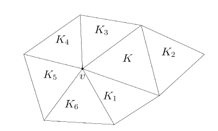
Figure 1. Graph for the illustration of the jumps in $\sigma_{K}^{\ell}$ defined in (3.4).

In Figure 1, we can see that $N_{e}=3$ for the element $K$ and $K_{1},K_{2},K_{3}$ are its adjacent neighbors, then we have:

$$\Big{(}[\![\partial^{\bm{\alpha}}w]\!]\Big{|}_{\bm{v}}\Big{)}^{2}=\big{[}(\partial^{\bm{\alpha}}w\big{|}_{K}-\partial^{\bm{\alpha}}w\big{|}_{K_{1}})^{2}+(\partial^{\bm{\alpha}}w\big{|}_{K}-\partial^{\bm{\alpha}}w\big{|}_{K_{3}})^{2}\big{]}\Big{|}_{\bm{v}}.$$

For more details we refer the reader to [18]. Throughout this paper, we take $\mathbf{R}^{-1}$ as follows

(3.7) $$\mathbf{R}^{-1}=\begin{pmatrix}c+un_{1}+vn_{2}&n_{1}&n_{2}\\ 2(un_{2}-vn_{1})&-2n_{2}&2n_{1}\\ c+un_{1}+vn_{2}&-n_{1}&-n_{2}\end{pmatrix},$$

where $c=\sqrt{gh}$.

The well-balanced property of the scheme (LABEL:wbofdg_scheme_2d) is as follows. The proof is similar to one-dimensional case, thus we omit it here.

Proposition 3.1.

The OFDG scheme (LABEL:wbofdg_scheme_2d) preserves the well-balanced property for the still water stationary state (3.2).

4. Numerical Tests

We test some one- and two-dimensional numerical examples and some benchmark problems to demonstrate the good performance of the proposed scheme in this section. The time discretization method in all numerical tests is the fourth order Runge-Kutta (RK4) method given in the Butcher tableau in Table 1, and the piecewise $P^{2}$ polynomial space is used unless otherwise specified. The gravitational constant $g=9.812m/s^{2}$.

Table 1. The Butcher tableau of the RK4.

0
1/2	1/2
1/2	0	1/2
1	0	0	1
	1/6	1/6	1/3	1/6

4.1. One-dimensional Problems

Example 1.

In this example, we consider two different bottom functions, one is smooth and another is discontinuous, to verify the proposed OFDG scheme maintain the well-balanced property over both bottoms. A smooth bottom is given by

(4.1) $$b(x)=5e^{-\frac{2}{5}(x-5)^{2}},0\leq x\leq 10,$$

and a discontinuous bottom is given by:

(4.4) $$b(x)=\left\{\begin{array}[]{cc}4&\text{ if }4\leq x\leq 8,\\ 0&\text{ otherwise},\end{array}\right.$$

The initial data satisfy the following stationary state:

$$h+b=10,\quad hu=0.$$

We compute both solutions until $t=0.5$ on the uniform mesh with $N=200$. In the simulations, we adopt the different precisions as shown in Table 2 to verify the well-balanced property. The errors for the water height $h$ and the discharge $hu$ in $L^{1}$, $L^{2}$ and $L^{\infty}$ norm are shown in Table 2. From Table 2, it is clearly to see that our scheme preserves the steady state in the round-off error level.

Table 2. $L^{1}$, $L^{2}$ and $L^{\infty}$ errors for the stationary solution with different precisions in Example 1.

		$L^{1}$ error		$L^{2}$ error		$L^{\infty}$ error
	precision	$h$	$hu$	$h$	$hu$	$h$	$hu$
smooth	single	1.372E-05	6.251E-05	1.424E-05	8.011E-05	2.193E-05	2.484E-04
	double	2.909E-14	8.752E-14	2.953E-14	1.091E-13	4.441E-14	2.599E-13
	quadruple	2.511E-32	7.277E-32	2.587E-32	8.911E-32	4.314E-32	2.945E-31
nonsmooth	single	1.376E-07	9.211E-06	3.351E-07	3.024E-05	1.431E-06	1.902E-04
	double	5.611E-16	7.560E-14	9.625E-16	1.258E-13	3.553E-15	6.733E-13
	quadruple	2.385E-33	9.419E-33	2.535E-33	2.051E-32	4.622E-33	1.187E-31

Example 2.

In this example we consider a still water steady state with non-flat bottom containing a wet/dry interface. The bottom topography is given by [19, 31]:

$$b(x)=\max(0,0.25-5(x-0.5)^{2}),\quad 0\leq x\leq 1.$$

The initial conditions are the stationary state solution:

$$h+b=\max(0.2,b),\quad hu=0.$$

The periodic boundary conditions are considered.

Note that in this case $h+b$ is no longer a constant function. In Figure 2, we plot the surface level $h+b$ and the bottom $b$. Since the water height $h=0$ if $0.4\leq x\leq 0.6$, then the numerical solution of $h$ easily becomes negative in this region. Thus the positive-preserving limiter [31] should be applied in this example. In the simulations, we use 200 uniform cells and compute the solution until $t=0.5$. We also use the different precisions to verify that $L^{1}$, $L^{2}$ and $L^{\infty}$ errors are at the level of round-off error, and present results in Table 3. From Figure 2 and Table 3, we can see that the well-balanced OFDG scheme (2.4) combined with the positive-preserving limiter does not destroy the well-balanced property.

Table 3. $L^{1}$, $L^{2}$ and $L^{\infty}$ errors for different precisions in Example 2.

	$L^{1}$ error		$L^{2}$ error		$L^{\infty}$ error
precision	$h$	$hu$	$h$	$hu$	$h$	$hu$
single	1.642E-08	7.765E-08	2.235E-08	1.499E-07	9.220E-08	8.003E-07
double	2.113E-15	1.160E-15	2.413E-15	1.514E-15	3.553E-15	5.500E-15
quadruple	8.253E-33	8.992E-33	1.046E-32	1.452E-32	1.914E-32	8.436E-32

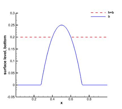
Figure 2. The surface level $h+b$ and the bottom $b$ for the stationary flow in Example 2.

Example 3.

The orders of accuracy for the well-balanced OFDG scheme (2.4) will be tested in this example. We consider the periodic boundary conditions and take the smooth bottom function:

$$b(x)=\sin^{2}(\pi x),~{}~{}x\in[0,1].$$

The initial data are given by

$$h(x,0)=5+e^{\cos(2\pi x)},~{}~{}(hu)(x,0)=\sin(\cos(2\pi x)),~{}~{}x\in[0,1].$$

Since we do not explicitly know the exact solutions of this problem, we adopt the a posteriori error $\|\mathbf{U}_{h}-\mathbf{U}_{\frac{h}{2}}\|$ as the numerical errors to compute the convergence rate. The terminal time is set to $t=0.1$ such that the solution is still smooth. We use $P^{1}$, $P^{2}$ and $P^{3}$ piecewise polynomials as finite element spaces. From Tables 4-5, the optimal convergence rate of all variables can be observed in each case.

Table 4. $h$’s numerical errors and orders in Example 3.

	$N$	$L^{1}$ error	order	$L^{2}$ error	order	$L^{\infty}$ error	order
$P^{1}$	10	5.242E-02	–	6.940E-02	–	1.964E-01	–
	20	1.461E-02	1.843	2.529E-02	1.456	8.430E-02	1.220
	40	3.068E-03	2.252	6.031E-03	2.068	2.343E-02	1.847
	80	5.806E-04	2.401	1.262E-03	2.257	7.800E-03	1.587
	160	1.050E-04	2.468	2.202E-04	2.519	1.495E-03	2.384
	320	2.220E-05	2.241	4.343E-05	2.342	3.045E-04	2.295
$P^{2}$	10	1.028E-02	–	1.952E-02	–	6.027E-02	–
	20	1.999E-03	2.362	4.547E-03	2.102	1.938E-02	1.637
	40	2.353E-04	3.086	6.390E-04	2.831	4.108E-03	2.238
	80	2.146E-05	3.455	6.934E-05	3.204	6.373E-04	2.689
	160	2.071E-06	3.373	6.798E-06	3.350	9.100E-05	2.808
	320	2.277E-07	3.185	7.575E-07	3.166	1.267E-05	2.845
$P^{3}$	10	3.372E-03	–	7.495E-03	–	2.794E-02	–
	20	4.070E-04	3.050	1.054E-03	2.830	5.064E-03	2.464
	40	2.815E-05	3.854	9.152E-05	3.526	6.525E-04	2.956
	80	1.237E-06	4.508	4.393E-06	4.381	4.369E-05	3.901
	160	6.439E-08	4.264	2.506E-07	4.132	3.245E-06	3.751
	320	3.778E-09	4.091	1.523E-08	4.040	1.931E-07	4.071

Table 5. $hu$’s numerical errors and orders in Example 3.

	$N$	$L^{1}$ error	order	$L^{2}$ error	order	$L^{\infty}$ error	order
$P^{1}$	10	2.571E-01	–	3.737E-01	–	8.432E-01	–
	20	8.741E-02	1.557	1.492E-01	1.325	5.076E-01	0.732
	40	2.537E-02	1.785	5.202E-02	1.520	2.033E-01	1.320
	80	4.726E-03	2.424	1.077E-02	2.272	6.570E-02	1.629
	160	8.391E-04	2.494	1.885E-03	2.514	1.290E-02	2.349
	320	1.763E-04	2.250	3.721E-04	2.341	2.643E-03	2.287
$P^{2}$	10	8.069E-02	–	1.568E-01	–	5.599E-01	–
	20	1.414E-02	2.512	3.342E-02	2.230	1.379E-01	2.021
	40	1.941E-03	2.865	5.386E-03	2.634	3.297E-02	2.065
	80	1.802E-04	3.430	5.939E-04	3.181	5.416E-03	2.606
	160	1.703E-05	3.403	5.818E-05	3.352	7.835E-04	2.789
	320	1.864E-06	3.192	6.481E-06	3.166	1.094E-04	2.840
$P^{3}$	10	2.888E-02	–	6.340E-02	–	2.117E-01	–
	20	3.487E-03	3.050	9.055E-03	2.808	4.477E-02	2.241
	40	2.422E-04	3.848	7.915E-04	3.516	5.728E-03	2.967
	80	1.066E-05	4.506	3.814E-05	4.375	3.895E-04	3.878
	160	5.570E-07	4.258	2.166E-06	4.138	2.877E-05	3.759
	320	3.252E-08	4.098	1.314E-07	4.043	1.705E-06	4.076

Example 4.

A small perturbation of a steady-state water is considered to examine the capability of capturing the small perturbation of the proposed scheme. This test example was proposed by LeVeque [15]. The bottom topography is given by:

$$b(x)=\left\{\begin{aligned} 0.25\Big{(}\cos\big{(}10\pi(x-1.5)\big{)}+1\Big{)}&\text{ if~{}~{} }1.4\leq x\leq 1.6,\\ 0\quad\quad&\text{ otherwise.}\end{aligned}\right.$$

We take the initial conditions as follows:

$$(hu)(x,0)=0,\quad h(x,0)=\left\{\begin{aligned} &1-b(x)+\epsilon&\text{ if~{}~{}}1.1\leq x\leq 1.2,\\ &1-b(x)&\text{ otherwise, }\end{aligned}\right.$$

where $\epsilon$ is a non-zero perturbation constant.

In Example 4, two perturbations $\epsilon=0.2$ (big pulse) and $\epsilon=0.001$ (small pulse) are used to test the scheme. For small $\epsilon$, this disturbance should generate two waves, propagating opposite directions at the characteristic speeds $\pm\sqrt{gh}$. It is difficult to involving such small perturbations of the water surface for many numerical methods [15]. We use $200$ uniform cells with simple transmissive boundary condition to compute the solution at time $t=0.2$. Figures 3 and 4 show the surface level and discharge for the big and small pulse cases respectively. For comparison, we also show the $2000$ cells solution as reference. We can see that our scheme successfully capture these waves on the relative coarse mesh and there are no obvious spurious numerical oscillations.

Figure 3. Example 4: $\epsilon=0.2$.

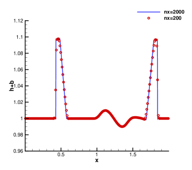
(a) Surface level

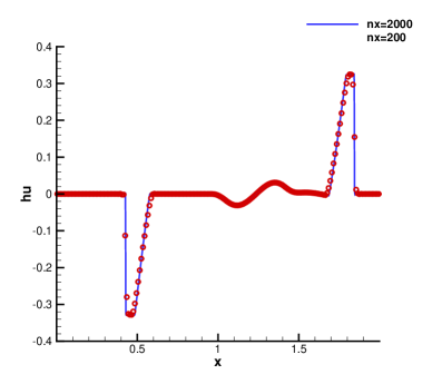
(b) The discharge

Figure 4. Example 4: $\epsilon=0.001$.

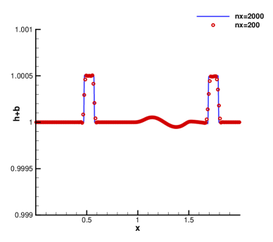
(a) Surface level

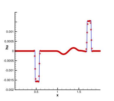
(b) The discharge

Example 5.

Next, we simulate the dam breaking problem over a rectangular bump [28]. We use this example to to test the scheme in the case of a rapidly varying flow over discontinuous bottom topography. The bed level is given with

$$b(x)=\left\{\begin{aligned} 8&\text{ if~{}~{} }|x-750|\leq 187.5,\\ 0&\text{ otherwise, }\end{aligned}\right.\quad x\in[0,1500].$$

The initial data are taken as follows

$$(hu)(x,0)=0,\quad h(x,0)=\left\{\begin{array}[]{cc}20-b(x)&\text{ if }x\leq 750,\\ 15-b(x)&\text{ otherwise.}\end{array}\right.$$

We compute the solutions at $t=15$ and $t=60$ by using $400$ uniform cells and use the results of $4000$ uniform cells as reference solutions. Figure 5 shows the numerical results have good resolution and non-oscillatory which agree well with the reference solution.

Figure 5. The dam breaking problem

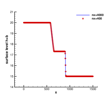
(a) $t=15$

(b) $t=60$

Example 6.

The last one-dimensional example is to study the convergence in time towards the steady flow over a bump. They are widely used to test numerical schemes for shallow water equations [12, 23, 28]. We take the bottom function as:

$$b(x)=\left\{\begin{array}[]{ll}0.2-0.05(x-10)^{2}&\text{ if }8\leq x\leq 12,\\ \quad\quad 0&\text{ otherwise },\end{array}\right.$$

The length of channel is $[0,25]$ and the initial conditions are given by

$$h(x,0)=0.5-b(x),\quad u(x,0)=0.$$

Theoretically, the flow can be subcritical or transcritical with or without a steady shock on different boundary conditions. We compute the solution until $t=200s$ on $200$ uniform meshes. We consider three types of boundary conditions:

a) Transcritical flow without a shock: The boundary condition is $hu=1.53m^{2}/s$ at $x=0$ and $h=0.66m$ at $x=25$.

We plot the surface level $h+b$ and discharge $hu$ in Figure 6. The numerical results show very good agreement with the analytical solution [12].

b) Transcritical flow with a shock: The boundary conditions are $hu=0.18m^{2}/s$ at $x=0$ and $h=0.33m$ at $x=25$.

Here we also plot the surface level $h+b$ and the discharge $hu$ in Figure 7. We can observe that the stationary shock appears on the surface. However, there is one overshoot near the jump on the discharge $hu$. Since our scheme is the still water well-balanced scheme not moving water well-balanced scheme, the similar result can also be found in [16].

c) Subcritical flow: The boundary conditions are $hu=4.42m^{2}/s$ at $x=0$ and $h=2m$ at $x=25$.

We also plot the surface level $h+b$ and the discharge $hu$ in Figure 8, and observe that the results have good performances comparing with the analytical solutions [12].

Figure 6. The transcritical flow without a shock

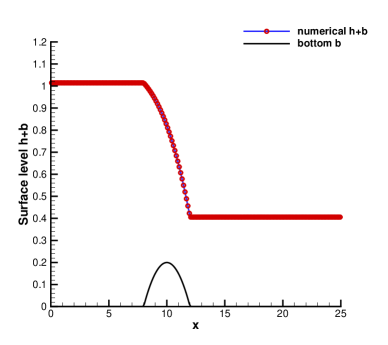
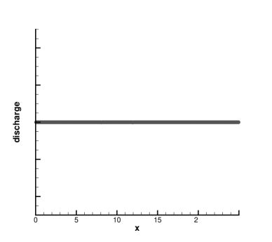
Figure 7. The transcritical flow with a shock

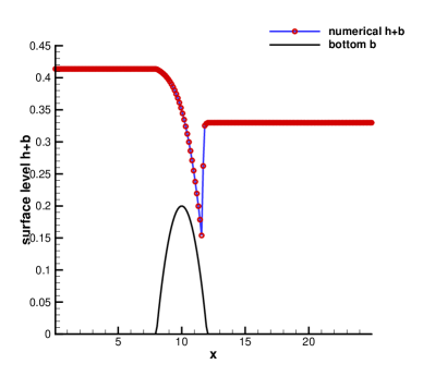
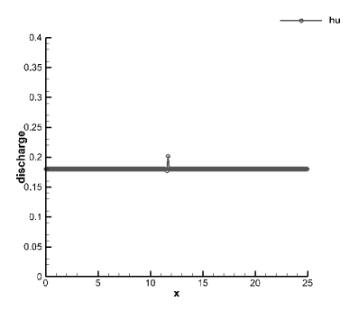
Figure 8. The steady subcritical flow

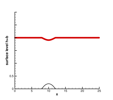
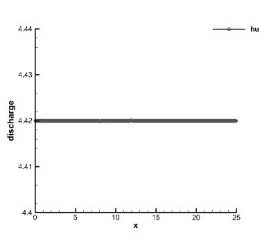
4.2. Two-dimensional Problems

Example 7.

Now let us test the well-balanced property in two dimensions. We consider a non-flat bottom as follows:

$$b(x,y)=0.8e^{-50((x-0.5)^{2}+(y-0.5)^{2})},\quad(x,y)\in[0,1]^{2}.$$

The initial stationary state is given by:

$$h(x,y)=1-b(x,y),\quad v(x,y,0)=u(x,y,0)=0.$$

We use the single, double and quadruple precisions to compute the numerical solutions up to time $t=0.1$ on the $100\times 100$ uniform mesh. It can be found that the scheme preserve the still water state from Table 6. For all numerical solutions, the $L^{2}$ and $L^{\infty}$ errors achieve the machine accuracy for different precisions, which confirms that the proposed scheme does preserve the well-balanced property in two-dimensions.

Table 6. $L^{2}$ and $L^{\infty}$ errors for the stationary solution with different precisions in Example 7.

	$L^{2}$ error			$L^{\infty}$ error
precision	$h$	$hu$	$hv$	$h$	$hu$	$hv$
single	4.034E-06	4.778E-06	4.823E-06	5.364E-06	4.227E-05	4.221E-05
double	1.892E-14	1.055E-14	1.041E-14	2.143E-14	7.965E-14	7.678E-14
quadruple	1.303E-32	9.898E-33	1.076E-32	1.483E-32	5.068E-32	4.904E-32

Example 8.

Next, we test the numerical accuracy of our schemes. Let us consider the following smooth bottom function and initial conditions:

$$b(x,y)=\sin(2\pi x)+\cos(2\pi y),\quad h(x,y,0)=10+e^{\sin(2\pi x)}\cos(2\pi y),$$

$$(hu)(x,y,0)=\sin(\cos(2\pi x))\sin(2\pi y),\quad(hv)(x,y,0)=\cos(2\pi x)\cos(\sin(2\pi y))\,,$$

where $(x,y)\in\Omega=[0,1]^{2}$ and the periodic boundary conditions are imposed.

We compute the solution at time $t=0.05$ before the shock appears in the solution. We still use the a posteriori error $\|\mathbf{U}_{h}-\mathbf{U}_{\frac{h}{2}}\|$ as numerical errors of $\mathbf{U}_{h}$. From Tables 7-9, we can observe the optimal convergence rate for all numerical solutions.

Table 7. $h$’s numerical errors and orders in Example 8.

	$N\times N$	$L^{1}$ error	order	$L^{2}$ error	order	$L^{\infty}$ error	order
$P^{1}$	$10\times 10$	9.202E-02	–	1.174E-01	–	4.798E-01	–
	$20\times 20$	2.110E-02	2.125	3.002E-02	1.968	1.783E-01	1.428
	$40\times 40$	4.318E-03	2.289	6.515E-03	2.204	5.325E-02	1.744
	$80\times 80$	9.109E-04	2.245	1.366E-03	2.254	1.292E-02	2.044
	$160\times 160$	2.120E-04	2.103	3.158E-04	2.113	2.879E-03	2.165
	$320\times 320$	5.167E-05	2.037	7.717E-05	2.033	7.884E-04	1.869
$P^{2}$	$10\times 10$	1.543E-02	–	2.472E-02	–	1.416E-01	–
	$20\times 20$	1.949E-03	2.985	4.203E-03	2.556	3.601E-02	1.975
	$40\times 40$	2.056E-04	3.245	4.995E-04	3.073	8.813E-03	2.031
	$80\times 80$	2.366E-05	3.119	6.080E-05	3.038	1.521E-03	2.534
	$160\times 160$	2.837E-06	3.060	7.543E-06	3.011	2.381E-04	2.676
	$320\times 320$	3.506E-07	3.017	9.414E-07	3.002	3.221E-05	2.886
$P^{3}$	$10\times 10$	3.722E-03	–	7.671E-03	–	4.978E-02	–
	$20\times 20$	2.475E-04	3.910	7.182E-04	3.417	1.087E-02	2.196
	$40\times 40$	1.496E-05	4.049	4.786E-05	3.908	1.544E-03	2.815
	$80\times 80$	8.752E-07	4.095	3.412E-06	3.810	1.477E-04	3.386
	$160\times 160$	5.075E-08	4.108	2.041E-07	4.063	9.506E-06	3.957
	$320\times 320$	3.087E-09	4.039	1.260E-08	4.018	5.972E-07	3.993

Table 8. $hu$’s numerical errors and orders in Example 8.

	$N$	$L^{1}$ error	order	$L^{2}$ error	order	$L^{\infty}$ error	order
$P^{1}$	$10\times 10$	4.287E-01	–	5.806E-01	–	2.048E+00	–
	$20\times 20$	9.343E-02	2.198	1.315E-01	2.143	5.354E-01	1.935
	$40\times 40$	1.684E-02	2.472	2.318E-02	2.504	1.102E-01	2.281
	$80\times 80$	3.208E-03	2.392	4.235E-03	2.453	2.275E-02	2.276
	$160\times 160$	7.060E-04	2.184	9.118E-04	2.215	5.696E-03	1.998
	$320\times 320$	1.683E-04	2.068	2.176E-04	2.067	1.434E-03	1.990
$P^{2}$	$10\times 10$	5.715E-02	–	8.461E-02	–	3.783E-01	–
	$20\times 20$	6.255E-03	3.192	9.655E-03	3.132	7.481E-02	2.338
	$40\times 40$	7.633E-04	3.035	1.191E-03	3.020	1.481E-02	2.336
	$80\times 80$	1.269E-04	2.588	1.982E-04	2.587	2.379E-03	2.638
	$160\times 160$	2.259E-05	2.490	3.646E-05	2.443	3.577E-04	2.734
	$320\times 320$	3.849E-06	2.553	6.413E-06	2.507	4.974E-05	2.846
$P^{3}$	$10\times 10$	1.333E-02	–	2.119E-02	–	1.246E-01	–
	$20\times 20$	1.027E-03	3.698	1.751E-03	3.597	2.477E-02	2.331
	$40\times 40$	7.112E-05	3.852	1.252E-04	3.806	2.645E-03	3.227
	$80\times 80$	4.532E-06	3.972	8.284E-06	3.917	1.969E-04	3.748
	$160\times 160$	2.703E-07	4.067	5.206E-07	3.992	1.513E-05	3.702
	$320\times 320$	1.477E-08	4.194	3.045E-08	4.096	1.035E-06	3.870

Table 9. $hv$’s numerical errors and orders in Example 8.

	$N$	$L^{1}$ error	order	$L^{2}$ error	order	$L^{\infty}$ error	order
$P^{1}$	$10\times 10$	6.891E-01	–	9.023E-01	–	2.335E+00	–
	$20\times 20$	1.596E-01	2.110	2.392E-01	1.916	1.043E+00	1.163
	$40\times 40$	3.281E-02	2.282	5.205E-02	2.200	3.485E-01	1.581
	$80\times 80$	6.891E-03	2.251	1.091E-02	2.254	9.071E-02	1.942
	$160\times 160$	1.611E-03	2.097	2.535E-03	2.106	2.115E-02	2.100
	$320\times 320$	3.923E-04	2.038	6.213E-04	2.029	5.564E-03	1.927
$P^{2}$	$10\times 10$	1.302E-01	–	2.193E-01	–	1.370E+00	–
	$20\times 20$	1.683E-02	2.952	3.687E-02	2.572	3.430E-01	1.998
	$40\times 40$	1.778E-03	3.243	4.268E-03	3.111	7.771E-02	2.142
	$80\times 80$	2.072E-04	3.101	5.186E-04	3.041	1.333E-02	2.544
	$160\times 160$	2.558E-05	3.018	6.440E-05	3.009	1.977E-03	2.753
	$320\times 320$	3.324E-06	2.944	8.107E-06	2.990	2.590E-04	2.932
$P^{3}$	$10\times 10$	3.380E-02	–	7.089E-02	–	5.048E-01	–
	$20\times 20$	2.265E-03	3.900	6.032E-03	3.555	1.060E-01	2.252
	$40\times 40$	1.501E-04	3.915	4.106E-04	3.877	1.369E-02	2.953
	$80\times 80$	9.436E-06	3.992	2.992E-05	3.778	1.212E-03	3.498
	$160\times 160$	5.554E-07	4.087	1.794E-06	4.060	7.502E-05	4.014
	$320\times 320$	3.287E-08	4.078	1.113E-07	4.010	4.624E-06	4.020

Example 9.

In the last example, we test the ability of the proposed scheme to capture the perturbation of the still water equilibrium in 2D. This example is widely used to test the well-balanced schemes, which is given by LeVeque [15]. The bottom function and the initial data are given by:

$$b(x,y)=0.8e^{-5(x-0.9)^{2}-50(y-0.5)^{2}}.$$

$$\begin{aligned} &h(x,y,0)=\left\{\begin{array}[]{ll}1-b(x,y)+0.01&\text{ if ~{}~{}}0.05\leq x\leq 0.15\\ 1-b(x,y)&\text{ otherwise }\end{array}\right.,\\ &(hu)(x,y,0)=(hv)(x,y,0)=0\,,\end{aligned}$$

where $(x,y)\in[0,2]\times[0,1]$.

We compute the numerical solutions on $200\times 100$ and $600\times 300$ uniform meshes respectively. Numerical solutions at different time are presented for comparison in Figure 9. These results demonstrate that our schemes can resolve the complex small features without obvious spurious oscillations.

Figure 9. The contours of the surface level $h+b$ for Example 9. Left: results with a $200\times 100$ uniform mesh. Right: results with a $600\times 300$ uniform mesh.

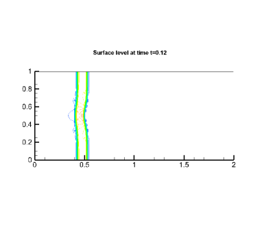
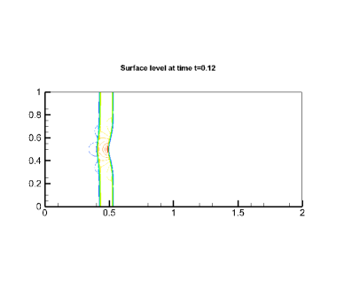
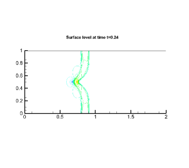
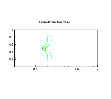
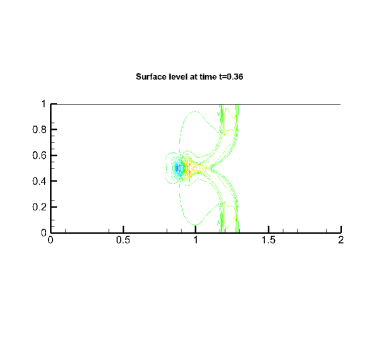
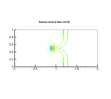
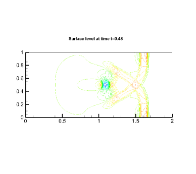
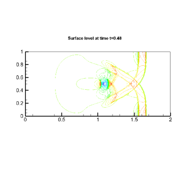
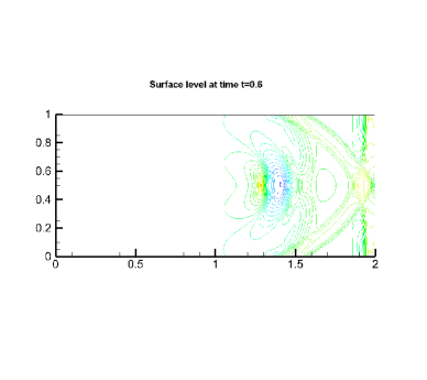
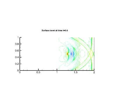
5. Concluding remarks

In this paper, we developed a well-balanced oscillation-free discontinuous Galerkin (OFDG) method for solving the shallow water equations. Following the idea of the OFDG method in [17, 18], we added the suitable extra damping terms to the existing well-balanced DG schemes proposed in [26, 28]. The extra damping terms are carefully designed so as to achieve the well-balanced property. It indicates the damping terms in the OFDG method is very flexible and they can be consistent with other good properties with some suitable modifications. The numerical experiments validated the proposed method had well performances for several benchmark problems. In our future plan, we will extend the current algorithm to the moving water steady state problems and other well-balanced dynamics such as the hyperbolic model of chemosensitive movement and the compressible Euler equations with gravitation, etc.

References

- [1] E. Audusse, F. Bouchut, M.-O. Bristeau, R. Klein and B. Perthame, A fast and stable well-balanced scheme with hydrostatic reconstruction for shallow water flows, SIAM J. Sci. Comput. 25 (2004), 2050 – 2065.
- [2] S. Bryson, Y. Epshteyn, A. Kurganov and G. Petrova, Well-balanced positivity preserving central-upwind scheme on triangular grids for the Saint-Venant system, ESAIM Math. Model. Numer. Anal. 45 (2011), 423 – 446.
- [3] D.S. Bale, R.J. Leveque, S. Mitran and J.A. Rossmanith, A wave propagation method for conservation laws and balance laws with spatially varying flux functions, SIAM J. Sci. Comput. 24 (2002), 955 – 978.
- [4] S. Bunya, E.J. Kubatko, J.J. Westerink and C. Dawson, A wetting and drying treatment for the Runge-Kutta discontinuous Galerkin solution to the shallow water equations, Comput. Methods Appl. Mech. Engrg. 198 (2009), 1548 – 1562.
- [5] O. Bokhove, Flooding and drying in discontinuous Galerkin finite-element discretizations of shallow-water equations. I. One dimension, J. Sci. Comput. 22/23 (2005), 47 – 82.
- [6] P.D. Bates and A.P.J. De Roo, A simple raster-based model for flood inundation simulation, J. Hydrol. 236 (2000), 54 – 77.
- [7] M.J. Briggs, C.E. Synolakis, G.S.Harkins and D.R. Green, Laboratory experiments of tsunami runup on a circular island, Pure Appl. Geophys. 144 (1995), 569 – 593.
- [8] A. Bermudez and M.E. Vazquez, Upwind methods for hyperbolic conservation laws with source terms, Comput. & Fluids 23 (1994), 1049 – 1071.
- [9] M.J. Castro, A. Pardo Milanés and C. Parés, Well-balanced numerical schemes based on a generalized hydrostatic reconstruction technique, Math. Models Methods Appl. Sci. 17 (2007), 2055 – 2113.
- [10] U.S. Fjordholm, S. Mishra and E. Tadmor, Well-balanced and energy stable schemes for the shallow water equations with discontinuous topography, J. Comput. Phys. 230 (2011), 5587 – 5609.
- [11] P. García-Navarro, J. Murillo, J. Fernández-Pato, I. Echeverribar and M. Morales-Hernández, The shallow water equations and their application to realistic cases, Environ. Fluid Mech. 19 (2019), 1235 – 1252.
- [12] N. Goutal and F. Maurel, Proceedings of the Second Workshop on Dam-Break Wave Simulation, Techinical Report HE-43/97/016/A, Electricité de France, Département Laboratoire National d’Hydraulique, Group Hydraulique Fluviale, 1997.
- [13] Y.-C. Hon, K.F. Cheung, X.-Z. Mao and E.J. Kansa, Multiquadric solution for shallow water equations, J. Hydraul. Eng. 125 (1999), 524 – 533.
- [14] G. Kesserwani and Q. Liang, Locally limited and fully conserved RKDG2 shallow water solutions with wetting and drying, J. Sci. Comput. 50 (2012), 120 – 144.
- [15] R.J. LeVeque, Balancing source terms and flux gradients on high-resolution Godunov methods: the quasi-steady wave propagation algorithm, J. Comput. Phys. 146 (1998), 346 – 365.
- [16] M. Li, P. Guyenne, F. Li and L. Xu, A positivity-preserving well-balanced central discontinuous Galerkin method for the nonlinear shallow water equations, J. Sci. Comput. 71 (2017), 994 – 1034.
- [17] Y. Liu, J. Lu and C.-W. Shu, An oscillation-free discontinuous Galerkin method for hyperbolic systems, submitted, https://www.brown.edu/research/projects/scientific-computing/sites/brown.edu.research.projects.scientific-computing/files/uploads/AN OSCILLATION-FREE ISCONTINUOUS GALERKIN METHOD FOR HYPERBOLIC SYSTEMS.pdf
- [18] J. Lu, Y. Liu and C.-W. Shu, An oscillation-free discontinuous Galerkin method for scalar hyperbolic conservation laws, SIAM J. Numer. Anal. 59 (2021), 1299 – 1324.
- [19] Q. Liang and F. Marche, Numerical resolution of well-balanced shallow water equations with complex source terms. Adv. Water Resour. 32 (2009), 873 – 884.
- [20] B. Perthame and C. Simeoni, A kinetic scheme for the Saint-Venant system with a source term, Calcolo 38 (2001), 201 – 231.
- [21] H. Qian, Z. Cao, H. Liu and G. Pender, New experimental dataset for partial dam-break floods over mobile beds, J. Hydraul. Res. 56 (201), 124 – 135.
- [22] C.-W. Shu, Discontinuous Galerkin methods: General approach and stability. Numerical solutions of partial differential equations, 149 – 201, Adv. Courses Math. CRM Barcelona, Birkhäuser, Basel, 2009.
- [23] M.E. Vazquez-Cendon, Improved treatment of source terms in upwind schemes for the shallow water equations in channels with irregular geometry, J. Comput. Phys. 148 (1999), 497 – 526.
- [24] X. Wen, W.-S. Don, Z. Gao and Y. Xing, Entropy stable and well-balanced discontinuous Galerkin methods for the nonlinear shallow water equations, J. Sci. Comput. 83 (2020).
- [25] Y. Xing and C.-W. Shu, High order finite difference WENO schemes with the exact conservation property for the shallow water equations, J. Comput. Phys. 208 (2005), 206 – 227.
- [26] Y. Xing and C.-W. Shu, High order well-balanced finite volume WENO schemes and discontinuous Galerkin methods for a class of hyperbolic systems with source terms, J. Comput. Phys. 214 (2006), 567 – 598.
- [27] Y. Xing and C.-W. Shu, High-order well-balanced finite difference WENO schemes for a class of hyperbolic systems with source terms, J. Sci. Comput. 27 (2006), 477 – 494.
- [28] Y. Xing and C.-W. Shu, A new approach of high order well-balanced finite volume WENO schemes and discontinuous Galerkin methods for a class of hyperbolic systems with source terms, Commun. Comput. Phys. 1 (2006), 100 – 134.
- [29] Y. Xing and C.-W. Shu, High-order finite volume WENO schemes for the shallow water equations with dry states, Adv. Water Resour. 34 (2011), 1026 – 1038.
- [30] Y. Xing and X. Zhang, Positivity-preserving well-balanced discontinuous Galerkin methods for the shallow water equations on unstructured triangular meshes, J. Sci. Comput. 57 (2013), 19 – 41.
- [31] Y. Xing, X. Zhang and C.-W. Shu, Positivity-preserving high order well-balanced discontinuous Galerkin methods for the shallow water equations, Adv. Water Resour. 33 (2010), 1476 – 1493.
- [32] Y. Xing and C.-W. Shu, A survey of high order schemes for the shallow water equations, J. Math. Study 47 (2014), 221 – 249.
- [33] J.G. Zhou, D.M. Causon, C.G. Mingham and D.M. Ingram, The surface gradient method for the treatment of source terms in the shallow-water equations, J. Comput. Phys. 168 (2001), 1 – 25.
- [34] X. Zhang and C.-W. Shu, On maximum-principle-satisfying high order schemes for scalar conservation laws, J. Comput. Phys. 229 (2010), 3091 – 3120.
- [35] X. Zhang and C.-W. Shu, On positivity-preserving high order discontinuous Galerkin schemes for compressible Euler equations on rectangular meshes, J. Comput. Phys. 229 (2010), 8918 – 8934.