Long-term variability of the composite galaxy SDSS J103911-000057: A candidate of true Type-2 AGN

Abstract

In the manuscript, the composite galaxy SDSS J103911-000057 (=SDSS J1039) is reported as a better candidate of true Type-2 AGN without hidden BLRs. None broad but only narrow emission lines detected in SDSS J1039  can be well confirmed both by the F-test technique and by the expected broad emission lines with EW smaller than 13.5Å  with 99% confidence level. Meanwhile, a reliable AGN power law component is preferred with confidence level higher than 7sigma in SDSS J1039. Furthermore, the long-term variability of SDSS J1039  from CSS can be well described by the DRW process with intrinsic variability timescale $\tau\sim 100{\rm days}$, similar as normal quasars. And, based on BH mass in SDSS J1039  through the $M_{\rm BH}-\sigma$ relation and on the correlation between AGN continuum luminosity and total H$\alpha$ luminosity, the expected broad H$\alpha$, if there was, could be re-constructed with line width about $300-1000{\rm km~{}s^{-1}}$ and with line flux about $666\times 10^{-17}{\rm erg~{}s^{-1}~{}cm^{-2}}$ under the Virialization assumption to BLRs, providing robust evidence to reject the probability that the intrinsic probable broad H$\alpha$ were overwhelmed by noises of the SDSS spectrum in SDSS J1039. Moreover, the SDSS J1039  does follow the same correlation between continuum luminosity and [O iii] line luminosity as the one for normal broad line AGN, indicating SDSS J1039  classified as a changing-look AGN at dim state can be well ruled out. Therefore, under the current knowledge, SDSS J1039  is a better candidate of true Type-2 AGN.

1 Introduction

Long-term variability tightly related to central BH (black hole) accreting process is one of fundamental characteristics of Type-1 AGN (broad line Active Galactic Nuclei) (Rees, 1984; Ulrich et al., 1997; Madejski & Sikora, 2016; Baldassare et al., 2020). The long-term variability, especially in optical band, can be well modeled by the Continuous AutoRegressive (CAR) process firstly proposed by Kelly et al. (2009) and then the improved damped random walk (DRW) process in Kozlowski et al. (2010); Zu et al. (2013); Kelly et al. (2014); Starkey et al. (2016); Zu et al. (2016). Based on the CAR/DRW process described long-term variability properties, AGN selections have been well applied, such as the discussed results in MacLeod et al. (2011); Kim et al. (2011); Choi et al. (2014); Tie et al. (2017); Sanchez-Saez et al. (2019); De Cicco et al. (2020). As well as the long-term optical variability properties, broad optical emission lines coming from central broad emission line regions (BLRs) are another fundamental characteristics of Type-1 AGN (Sulentic et al., 2000; Czerny & Hryniewicz, 2011; Baskin & Laor, 2018; Zaw et al., 2019). Combining the long-term variability with broad line emission features, Type-1 AGN can be well identified.

Besides Type-1 AGN with apparent broad emission lines and also apparent long-term variability, there is one another kind of AGN: the Type-2 AGN with only narrow emission lines coming from narrow line regions (NLRs) in optical spectra. Properties of narrow emission lines have been well applied to detect central AGN activities in narrow emission-line galaxies, such as the results on the ongoing improved BPT diagrams (Baldwin et al., 1981; Kauffmann et al., 2003; Groves et al., 2006; Kewley et al., 2006; Cid Fernandes et al., 2011; Juneau et al., 2014; Kashino et al., 2017; Kewley et al., 2019; Zhang et al., 2020). Moreover, based on the discovery of polarized broad permitted lines in Antonucci & Miller (1985); Tran (2001, 2003); Nagao et al. (2004); Savic et al. (2018) in some Type-2 AGN, the well-known Unified Model in Antouncci (1993); Netzer (2015); Audibert et al. (2017) has been proposed and well accepted to explain the different observational optical phenomena mainly due to orientation effects of central dust torus. Therefore, under the framework of the Unified model, Type-1 AGN and Type-2 AGN have the same central geometric structures, but central engine and BLRs hidden in Type-2 AGN.

However, based on the interesting work on detecting polarized broad emission lines in Type-2 AGN, especially on the pioneer work in Tran (2001), there is one special kind of AGN: true Type-2 AGN (or Type-2 AGN with none hidden-BLRs, or BLRs-less AGN, or unobscured Type-2 AGN, or naked AGN in literature), with no expected hidden central BLRs. Tran (2001, 2003) have shown spectropolarimetric results of about 30 Seyfert 2 galaxies with no hidden BLRs, due to lack of polarized broad emission lines. Shi et al. (2010) have reported two strong candidates of true Type-2 AGN, NGC3147 and NGC4594, which have few X-ray extinctions and have the upper limits on the broad emission line luminosities are two orders of magnitude lower than the average of typical Type-1 AGN, leading to the conclusion that "true Type-2 AGN do exist but they are very rare". Barth et al. (2014) have shown that there is possibility that a very small number of Type-2 quasar with strong g-band variability might be true Type-2 AGN. Zhang (2014) have shown a sample of candidates of true Type-2 AGN with both the long-term variability and the expected reliable power law components in their spectra in SDSS (Sloan Digital Sky Survey). Li et al. (2015) have reported a candidate of true Type-2 AGN, SDSS J0120, with long-term variability but none-detected broad emission lines. More recently, Pons & Watson (2016) have shown a sample of candidates of true Type-2 AGN based on properties of unobscured X-ray emissions.

Studying on true Type-2 AGN can provide further clues on formation or suppression of central BLRs in AGN, such as the proposed theoretical models on the nature of true Type-2 AGN in Nicastro et al. (2003); Elitzur & Ho (2009); Cao (2010); Elitzur & Netzer (2016), strongly indicating disappearance of central BLRs depends on physical properties of central AGN activities and/or depends on properties of central dust obscuration. Nicastro et al. (2003) have shown that "the absence or presence of central BLRs can be well regulated by accretion rate, assumed that the BLRs are formed by accretion disk instabilities occurring in proximity of the critical radius at which the disk changes from gas pressure dominated to radiation pressure dominated". Elitzur & Ho (2009) have proposed a disk-wind scenario in AGN to predict the disappearance of the central BLRs at luminosities lower than $5\times 10^{39}M_{7}^{2/3}{\rm erg~{}s^{-1}}$ with $M_{7}$ as central BH mass in unit of $10^{7}{\rm M_{\odot}}$. Cao (2010) has shown that "disappearance of central BLRs associated with the outflows from the accretion disks can be expected in AGN with Eddington ratio smaller than 0.001, because the inner small cold disk is evaporated completely in the advection dominated accretion flows (ADAF) and outer thin accretion disk may be suppressed by the ADAF". Elitzur & Netzer (2016) have shown that "true Type-2 AGN should have higher luminosities than $4\times 10^{46}{\rm erg~{}s^{-1}}$ considering mass conservations in the disk outflows".

Commonly, disappearance of broad emission lines could also be probably due to lower spectral quality, such as the results in Mrk573 and NGC3147. Mrk573 has been classified as a true Type-2 AGN in Tran (2001). However, Nagao et al. (2004) have shown the clearly detected polarized broad Balmer lines, leading Mrk573 as a normal Type-2 AGN with central hidden BLRs. Similarly, NGC3147 has been previously classified as a true Type-2 AGN in Shi et al. (2010); Bianchi et al. (2012) through both spectropolarimetric results and unobscured X-ray emission properties, however Bianchi et al. (2019) more recently have clearly detected double-peaked broad H$\alpha$ in high quality HST spectrum. Meanwhile, Ichikawa et al. (2015) have shown that none detected polarized broad emission lines in candidates of some true Type-2 AGN are probably due to effects of less scattering medium due to the reduced scattering volume given the small torus opening angle and/or due to effects of the increased torus obscurations.

There is so-far no definite conclusions on the very existence of true Type-2 AGN, neither clear conclusion on the physical nature of true Type-2 AGN, but more candidates of true Type-2 AGN can provide further clues on intrinsic physical properties of true Type-2 AGN. In the manuscript, we report one new candidate of true Type-2 AGN in SDSS J103911-000057 (=SDSS J1039) through both its apparent long-term optical variability and high-quality spectroscopic features having no broad emission lines. The manuscript is organized as follows. Section 2 presents our main results on spectroscopic emission line features and the properties of optical long-term V-band variability of SDSS J1039. Necessary discussions are shown in Section 3. Section 4 gives the final conclusions. And in this manuscript, we have adopted the cosmological parameters of $H_{0}=70{\rm km\cdot s}^{-1}{\rm Mpc}^{-1}$, $\Omega_{\Lambda}=0.7$ and $\Omega_{\rm m}=0.3$.

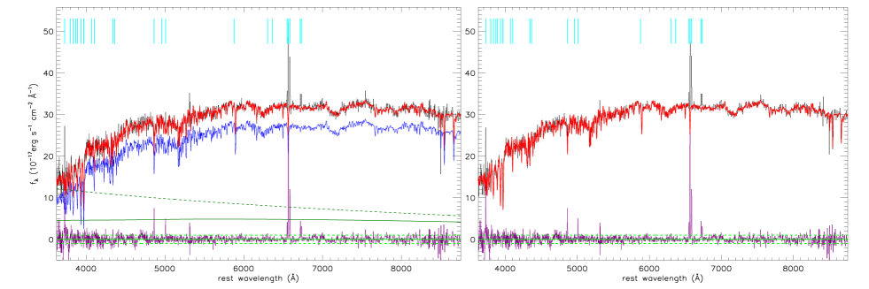
Figure 1: SDSS spectrum of SDSS J1039  and the determined host galaxy contributions by the SSP method with (in left panel) and without (in right panel) considerations of a power law component. In each panel, from top to bottom, solid black line shows the observed SDSS spectrum, solid red line shows the determined best descriptions to the spectrum with emission lines being masked out, solid purple line shows the line spectrum after subtractions of the best descriptions, horizontal solid green line shows $f_{\lambda}=0$, and horizontal dashed green lines show $f_{\lambda}=\pm 1$, respectively. In the left panel, solid blue line shows the determined stellar lights of host galaxy, solid dark green line shows the determined reddened AGN power law component, dashed dark green line shows the reddening corrected AGN power component. In each panel, from left to right, the vertical cyan lines mark the following emission features which are being masked out when the SSP method is running, including [O ii]$\lambda 3727$Å , H$\theta$, H$\eta$, [Ne iii]$\lambda 3869$Å, He i$\lambda 3891$Å, Calcium K line, [Ne iii]$\lambda 3968$Å, Calcium H line, [S ii]$\lambda 4070$Å, H$\delta$, H$\gamma$, [O iii]$\lambda 4364$Å, H$\beta$, [O iii]$\lambda 4959,5007$Å, He i$\lambda 5877$Å, [O i]$\lambda 6300,6363$Å, [N ii]$\lambda 6548$Å, H$\alpha$, [N ii]$\lambda 6583$Å, and [S ii]$\lambda 6716,6732$Å, respectively.

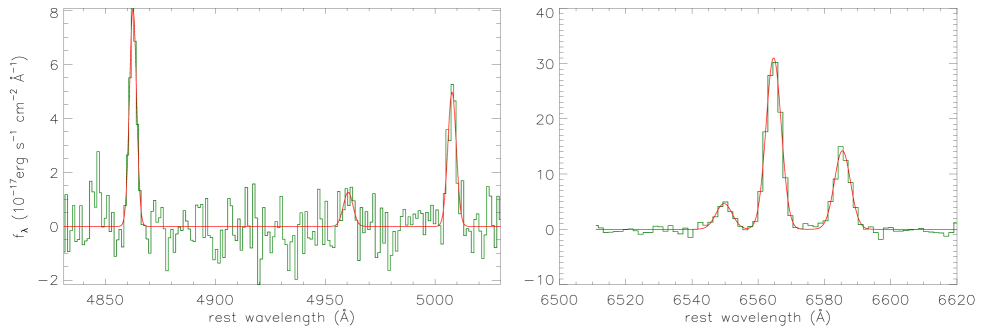
Figure 2: The Gaussian fitted results to the emission lines around H$\beta$ (left panel) and around H$\alpha$ (right panel). In each panel, solid line in dark green shows the line spectrum, and solid red line shows the best fitting results.

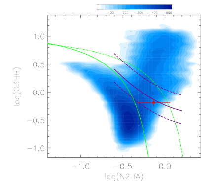
Figure 3: Properties of SDSS J1039  (solid red circle plus error bars) in the BPT diagram of O3HB versus N2HA. Solid and dashed green lines show the dividing lines reported in Kauffmann et al. (2003) and in Kewley et al. (2001) between HII galaxies, composite galaxies and AGN. Solid purple line and dashed purple lines show the dividing line and area for composite galaxies determined in our recent work in Zhang et al. (2020). The contour is created by emission line properties of more than 35000 narrow emission-line galaxies discussed in Zhang et al. (2020) collected from SDSS DR15. Corresponding number densities to different colors are shown in the color bar.

2 Spectroscopic and long-term photometric variability properties of SDSS J1039

SDSS J1039  at redshift 0.0499 is a main galaxy in SDSS DR16 (Ahumada et al., 2020), with the apparent optical Petroson magnitudes of 20.05, 18.01, 17.21, 16.78, 16.46 at u, g, r, i and z bands, respectively. And based on the SDSS provided inverse concentration indices (ratio of the two Petrosian radii $r50/r90$ with $r50$ as half light radius and $r90$ as 90% light radius) of 0.67, 0.61, 0.60, 0.59, 0.60 at u, g, r, i and z bands, SDSS J1039  is a late-type galaxy, based on the discussed results in Strateva et al. (2001); Shimasaku et al. (2001) (see also descriptions in https://www.sdss.org/dr12/algorithms/classify/). Fig. 1 shows the galactic reddening corrected spectrum (PLATE-MJD-FIBERID=0274-51913-0232) of SDSS J1039  observed in January 2001 with total exposure time of 5400 seconds and with median signal-to-noise $SN\sim 34$.

It is clear that the SDSS spectrum of SDSS J1039  has apparent host galaxy contributions. In order to check whether is there an AGN component and in order to well measure emission line properties, host galaxy contributions should be firstly determined. The commonly accepted SSP (Simple Stellar Population) method is well applied. The SSP method has been firstly proposed in Bruzual & Charlot (2003), to describe observed spectra of galaxies by stellar population synthesis. Then, the SSP method has been widely applied to determined the star formation history, metallicity and dust content of galaxy, such as the detailed discussions in Kauffmann et al. (2003); Cid Fernandes et al. (2005); Cappellari (2017), etc. Here, the 39 simple stellar population templates from Bruzual & Charlot (2003) have been exploited, which can be used to well-describe the characteristics of almost all the SDSS galaxies as discussed in Bruzual & Charlot (2003). Meanwhile, there is an additional component, a power law component $\alpha\times\lambda^{\beta}$, applied to describe the intrinsic AGN continuum emissions which can be well confirmed by the following shown long-term variability. Moreover, the intrinsic reddening effects can be well considered by a parameter of $E(B-V)$. Then, similar as what we have done in Zhang (2014); Zhang et al. (2019); Zhang (2021a, b), with the emission lines listed in http://classic.sdss.org/dr1/algorithms/speclinefits.html#linelist being masked out by full width at zero intensity about 450${\rm km~{}s^{-1}}$, the observed SDSS spectrum of SDSS J1039  can be well described by the broadened and reddened SSPs (the broadening velocity as the stellar velocity dispersion) plus the reddened power law component through the Levenberg-Marquardt least-squares minimization technique.

When the model functions are applied, there are 43 model parameters, 39 strengthen factors with zero as the starting values for the 39 SSPs, the broadening velocity $\sigma_{\star}$ with ${\rm 100km~{}s^{-1}}$ as the starting value, $\alpha$ and $\beta$ for the power law component with zero as the starting values, and the parameter of $E(B-V)$ with zero as the starting value. Then, the best descriptions to the spectrum of SDSS J1039  can be well determined, leading the determined $\chi^{2}/Dof$ (the summed squared residuals divided by degree of freedom) to be about $\chi^{2}_{2}/Dof_{2}\sim 3925.5/3561$, and the determined stellar velocity dispersion to be about $\sigma_{\star}\sim 76.5\pm 4.3{\rm km~{}s^{-1}}$, and the determined parameter $E(B-V)$ to be about 0.22, and the determined reddened power law component described by $4.67\times(\lambda/5100\text{\AA})^{-0.04}$. The best-fitting results are shown in the left panel of Fig. 1. Based on the well determined host galaxy contributions and the power law component, the continuum intensity ratio at 5100Å  is about 4.6 of the continuum emissions from stellar lights to the AGN emissions.

Moreover, the commonly accepted F-test technique is applied to determine whether the fitting procedure above determined power law component is necessary enough. Without considering the power law component, only the broadened SSPs are applied to describe the observed SDSS spectrum of SDSS J1039  with emission lines being masked out. Through the Levenberg-Marquardt least-squares minimization technique, the best descriptions to the SDSS spectrum of SDSS J1039  by only the SSPs are shown in the right panel of Fig. 1, leading the determined $\chi^{2}/Dof$ to be about $\chi^{2}_{1}/Dof_{1}\sim 3953.6/3563$, and the determined stellar velocity dispersion to be about $\sigma_{\star}\sim 81.2\pm 4.1{\rm km~{}s^{-1}}$, and the determined $E(B-V)$ to be about 0.26. Based on the different $\chi^{2}/Dof$ for the different model functions with and without considerations of the power law component, the calculated $F_{p}$ value is about

$$F_{p}=\frac{\frac{\chi^{2}_{1}-\chi^{2}_{2}}{Dof_{1}-Dof_{2}}}{\chi^{2}_{2}/Dof_{2}}\sim 12.75$$ (1)

. Based on $Dof_{1}-Dof_{2}$ and $Dof_{2}$ as number of Dofs of the F distribution numerator and denominator, the expected value from the statistical F-test with confidence level higher than 99.9997% will be near to $F_{p}$. Therefore, the power law component can be well accepted with confidence level higher than 99.9997% (higher than 7sigma).

Table 1: Line parameters of emission lines of SDSS J1039

Line	$\lambda_{0}$	$\sigma$	flux
H$\alpha$	6564.65$\pm$0.06	2.29$\pm$0.05	178.6$\pm$3.6
H$\beta$	4862.59$\pm$0.14	1.61$\pm$0.14	32.6$\pm$2.5
[O iii]$\lambda 5007$Å	5007.68$\pm$0.27	1.92$\pm$0.26	23.9$\pm$2.9
[N ii]$\lambda 6583$Å	6585.41$\pm$0.11	2.43$\pm$0.11	86.7$\pm$3.3

Notice: The second, third and fourth columns show the central wavelength in unit of Å in rest frame, the line width (second moment) in unit of Å and the line flux in unit of $10^{-17}{\rm erg~{}s^{-1}~{}cm^{-2}}$.

After subtractions of the stellar lights and the power law component shown in the left panel of Fig. 1, the emission lines in the line spectrum can be well measured by narrow Gaussian functions (second moment smaller than 400${\rm km~{}s^{-1}}$). There are three narrow Gaussian functions are applied to describe the narrow H$\beta$ and [O iii]$\lambda 4959,5007$Å  doublet within the rest wavelength from 4830Å  to 5030Å, and three narrow Gaussian functions are applied to describe the narrow H$\alpha$ and [N ii]$\lambda 6548,6583$Å  doublet within the rest wavelength from 6510Å  to 6620Å. Then, through the Levenberg-Marquardt least-squares minimization technique, the best fitting results to the emission lines are shown in Fig. 2 with the determined $\chi^{2}/Dof$ to be about $\chi^{2}_{1}/Dof_{1}\sim 200.446/231$. When the model functions are applied, three parameters of each Gaussian function are free parameters, and there are no further restrictions on the model parameters besides the restrictions that line fluxes are not smaller than zero.

Why it is not necessary to consider broad Balmer components? We answer the question by the F-test statistical technique. Besides the pure narrow Gaussian functions applied above, two broad Gaussian functions (second moment larger than 400${\rm km~{}s^{-1}}$) with central wavelengths fixed to 4862Å  and 6564Å  are applied to describe the probable broad H$\beta$ and broad H$\alpha$. Then, within the rest wavelength from 4830Å  to 5030Å  and from 6510Å  to 6620Å, the emission lines in the line spectrum are described again by the new model functions through the Levenberg-Marquardt least-squares minimization technique, leading the determined $\chi^{2}/Dof$ to be about $\chi^{2}_{2}/Dof_{2}\sim 199.758/227$. Then, the calculated $F_{p}$ value is about

$$F_{p}=\frac{\frac{\chi^{2}_{1}-\chi^{2}_{2}}{Dof_{1}-Dof_{2}}}{\chi^{2}_{2}/Dof_{2}}\sim 0.195$$ (2)

. Based on $Dof_{1}-Dof_{2}=4$ and $Dof_{2}=227$ as number of Dofs of the F distribution numerator and denominator, the expected value from the statistical F-test with confidence level around 6% will be near to $F_{p}$. Therefore, we can safely accepted that it is not necessary to consider the broad Balmer emission components in SDSS J1039, due to the lower confidence level around 6%.

The measured line parameters are listed in Table 1. The flux ratios of [O iii]$\lambda 5007$Å  to narrow H$\beta$ (O3HB) and of [N ii]$\lambda 6583$Å  to narrow H$\alpha$ (N2HA) are about 0.73 and 0.64, respectively, indicating SDSS J1039  is a standard composite galaxy, based on the dividing lines reported in Kewley et al. (2001); Kauffmann et al. (2003); Kewley et al. (2006) and reported regions for composite galaxies in Zhang et al. (2020). Fig. 3 shows properties of SDSS J1039  in the BPT diagram of N2HA versus O3HB, leading SDSS J1039  to be a well classified composite galaxy with a weak AGN component with confidence levels higher than 7sigma. In order to confirm SDSS J1039  as a true Type-2 AGN, variability properties can provide further and robust evidence, combining with the spectroscopic properties.

There are four reasonable explanations on the spectroscopic features having no broad emission lines of one narrow emission-line object. First, the narrow emission-line object is a normal Type-2 AGN with hidden central BLRs. Second, the narrow emission-line object is a true Type-2 AGN with lack of central BLRs. Third, the narrow emission-line object is a quiescent galaxy with no considerations of broad emission lines. Fourth, the narrow emission-line object is an AGN but with central BLRs seriously obscured. Long-term variability, as one of fundamental characteristics of broad line AGN (no variability in quiescent galaxies), will provide robust evidence to confirm which explanation is preferred. If there was apparent long-term variability indicating the central engine of AGN can be directly observed, both the second and the fourth explanation could be preferred. Certainly, if there was no apparent long-term variability, it would be hard to confirm which explanation is preferred. In the SDSS J1039, the seriously obscured central BLRs can also be well ruled out, because the confirmed apparent AGN power law component should lead to expected apparaent broad emission lines as well discussed re-constructed broad Balmer lines in the subsection 3.1, against the spectroscopic features with no broad emission lines. Therefore, if there was apparent long-term variability in SDSS J1039, only the second explanation can be well preferred, leading to the conclusion of lack of central BLRs in SDSS J1039.

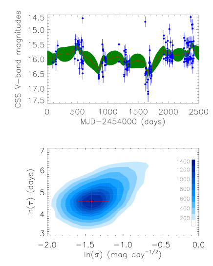
Figure 4: Top panel shows the CSS V-band light curve shown as solid blue circles plus error bars of SDSS J1039  and the determined best descriptions shown as solid red line by the public JAVELIN code. In top panel, area covered by dark green shows the corresponding 1sigma confidence bands to the best descriptions. Bottom panel shows the MCMC determined two-dimensional projected posterior distributions of the two DRW parameters of $\sigma$ in unit of ${\rm mag~{}day^{-0.5}}$ and $\tau$ in unit of days. In bottom panel, solid circle plus error bars show the accepted values and corresponding uncertainties.

The 6.4years-long photometric V-band light curve of SDSS J1039  can be collected from CSS (Catalina Sky Survey) (Drake et al., 2009) and shown in Fig. 4. Then, the widely accepted DRW/CAR process is applied to check the variability properties of SDSS J1039, because the DRW/CAR process has been proved to be a preferred modeling process to describe AGN intrinsic variability, such as the well discussed results in MacLeod et al. (2010); Bailer-Jones (2012); Andrae, Kim & Bailer-Jones (2013); Zu et al. (2013). Kelly et al. (2009) have firstly proposed the CAR process (Brockwell & Davis, 2002) to describe the AGN intrinsic variability, and found that the AGN intrinsic variability timescales are consistent with disk orbital or thermal timescales. Kozlowski et al. (2010) have provided an improved robust mathematic method to estimate the DRW process parameters, and found that AGN variability could be well modeled by the DRW process. Then, Zu et al. (2011) have provided a public code of JAVELIN (http://www.astronomy.ohio-state.edu/~yingzu/codes.html) (Just Another Vehicle for Estimating Lags In Nuclei) based on the method in Kozlowski et al. (2010). Here, the JAVELIN code is accepted to describe the long-term variability of SDSS J1039. Through the MCMC (Markov Chain Monte Carlo, Foreman-Mackey et al. (2013)) analysis with the uniform logarithmic priors of the DRW process parameters of $\tau$ in unit of days and $\sigma$ in unit of ${\rm mag~{}day^{-0.5}}$ covering every possible corner of the parameter space ($0~{}<~{}\tau/{\rm days}~{}<~{}1e+5$ and $0~{}<~{}\sigma/({\rm mag~{}day^{-0.5}})~{}<~{}1e+2$), the posterior distributions of the DRW process parameters can be well determined, similar as what we have done in Zhang & Feng (2017a). The best descriptions to the light curve of SDSS J1039  by the JAVELIN code are shown in the top panel of Fig. 4. And the MCMC determined two-dimensional projected posterior distributions of $\ln(\sigma/({\rm mag~{}day^{-0.5}}))$ and $\ln(\tau/{\rm days})$ are shown in the bottom panel of Fig. 4, with accepted $\ln(\sigma/({\rm mag~{}day^{-0.5}}))\sim-1.41_{-0.12}^{+0.31}$ and $\ln(\tau/{\rm days})\sim 4.57_{-0.39}^{+0.81}$ ($\tau\sim 97{\rm days}$). Comparing with the reported values of $\tau/{\rm days}$ in SDSS quasars in MacLeod et al. (2010) and in the sample of quasars in Kelly et al. (2009), $\tau\sim 97{\rm days}$ in SDSS J1039  is a common value in quasars, indicating the long-term variability is connected to intrinsic AGN activities in SDSS J1039.

Based on the DRW process described long-term variability, an intrinsic AGN component can be preferred, which also can be supported by the detected AGN power law components in the SDSS spectrum. Therefore, combining variability properties with the spectroscopic properties without broad emission lines, SDSS J1039  can be well accepted as a candidate of true Type-2 AGN.

3 Main discussions

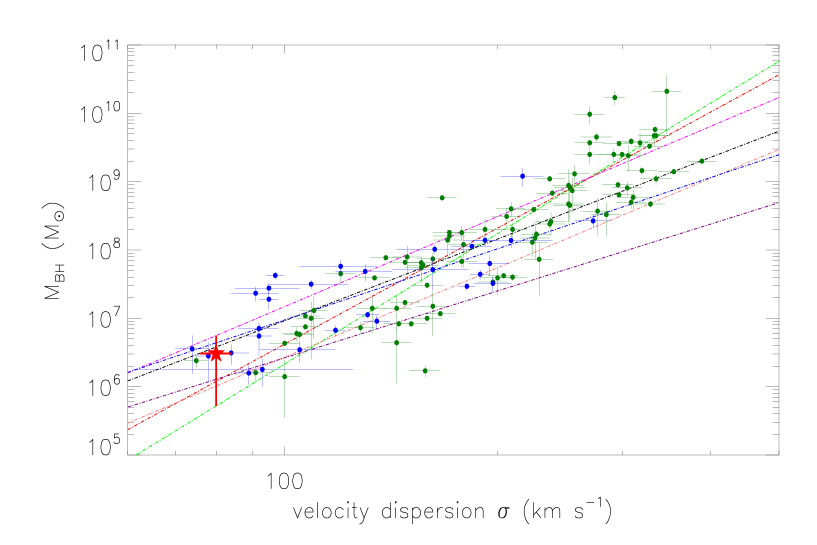
Figure 5: On the correlation between stellar velocity dispersion and BH mass for both quiescent galaxies and AGN. Solid circles in dark green and in blue show the measured results for the 89 quiescent galaxies well discussed in Savorgnan & Graham (2015) and the 29 RM (reverberation-mapped) AGN well discussed in Woo et al. (2015), respectively. Dot-dashed lines in green, in red, in magenta, in black, in pink, in purple and in blue represent the reported $M_{\rm BH}-\sigma$ relations determined through the quiescent galaxies in Savorgnan & Graham (2015), in McConnell & Ma (2013), in Kormendy & Ho (2013) and through the RM AGN in Woo et al. (2015), the RM AGN with classical bulges in Ho & Kim (2014), the RM AGN with pseudobulges in Ho & Kim (2014) and the RM AGN in Woo et al. (2013), respectively. And the solid five-point-star in red shows the measured results of the SDSS J1039  with BH mass about $(3.1\pm 2.5)\times 10^{6}{\rm M_{\odot}}$ and with the measured $\sigma_{\star}\sim 80{\rm km~{}s^{-1}}$.

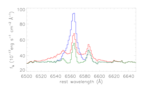
Figure 6: The expected spectroscopic properties around H$\alpha$ with considering the re-constructed broad H$\alpha$ through the Virialization assumptions to BLRs. Solid line in dark green shows the SDSS spectrum of SDSS J1039  within rest wavelength from 6500Å  to 6650Å. Solid blue line shows the expected spectroscopic properties, if there was the expected broad H$\alpha$ re-constructed with second moment of $303{\rm km~{}s^{-1}}$ and line flux of $666\times 10^{-17}{\rm erg~{}s^{-1}~{}cm^{-2}}$. Solid red line shows the expected spectroscopic properties, if there was the expected broad H$\alpha$ re-constructed with second moment of $996{\rm km~{}s^{-1}}$ and line flux of $666\times 10^{-17}{\rm erg~{}s^{-1}~{}cm^{-2}}$.

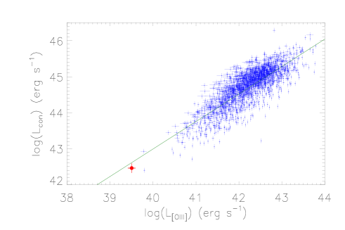
Figure 7: On the correlation between continuum luminosity and total [O iii] line luminosity. Solid blue dots plus error bars are the results for Type-1 AGN discussed in Zhang & Feng (2017). Solid red circle plus error bars are the results for the SDSS J1039.

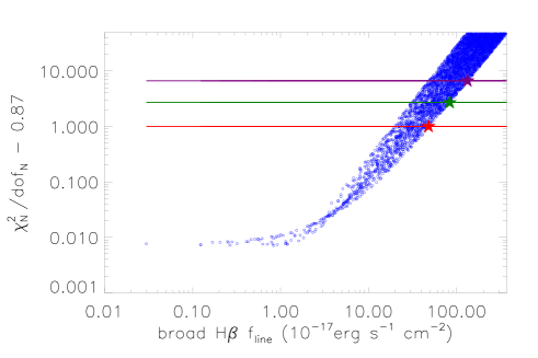
Figure 8: Dependence of $\chi^{2}_{N}/dof_{N}-0.87$ on the input line flux $f_{line}$ of expected broad H$\beta$. Open blue circles are the results from 5000 randomly collected values of $\sigma_{line}$ and $f_{line}$. The horizontal lines in red, in green and in purple show $\chi^{2}_{N}/dof_{N}-0.87=1$ (68% confidence level), $\chi^{2}_{N}/dof_{N}-0.87=2.7$ (90% confidence level) and $\chi^{2}_{N}/dof_{N}-0.87=6.63$ (99% confidence level), respectively. The five-point-stars in red, in green and in purple show the upper limits of $f_{line}$ with confidence levels of 68%, 90% and 99%, respectively.

Table 2: The reported $M_{\rm BH}-\sigma$ relations in literature

obj	N	$\alpha_{BH}$	$\beta_{BH}$	Ref
QG	89	8.24$\pm$0.10	6.34$\pm$0.80	Savorgnan & Graham (2015)
QG	72	8.32$\pm$0.05	5.64$\pm$0.32	McConnell & Ma (2013)
QG	51	8.49$\pm$0.05	4.38$\pm$0.29	Kormendy & Ho (2013)
RA	29	8.16$\pm$0.18	3.97$\pm$0.56	Woo et al. (2015)
RAC	16	7.74$\pm$0.13	4.35$\pm$0.58	Ho & Kim (2014)
RAP	14	7.40$\pm$0.19	3.25$\pm$0.76	Ho & Kim (2014)
RA	25	8.02$\pm$0.15	3.46$\pm$0.61	Woo et al. (2013)

Notice: The first column shows what objects are used to determine the $M_{\rm BH}-\sigma$ relation: QG for Quiescent galaxies, RA for reverberation mapped AGN, RAC for reverberation mapped AGN with classical bulges, RAP for reverberation mapped AGN with pseudobulges. The second column shows number of the used objects. The third and the forth columns list the values of $\alpha_{BH}$ and $\beta_{BH}$, respectively. The fifth column shows the corresponding reference.

3.1 Properties of re-constructed broad emission lines, if there were broad emission lines overwhelmed in the SDSS spectrum

In the subsection, two methods are applied to determine whether are there expected broad emission lines overwhelmed in the SDSS spectrum of the SDSS J1039. One method is to re-construct broad H$\alpha$ after considering Virialization assumptions to BLRs. The other method is applied to determine the upper limits of line flux of the expected broad emission lines in the SDSS J1039.

The first method is applied as follows. Based on the measured stellar velocity dispersion about $\sigma_{\star}\sim 80{\rm km/s}$, the BH mass can be estimated through the well-known $M_{\rm BH}-\sigma$ relation,

$$\log(\frac{M_{\rm BH}}{\rm M_{\odot}})~{}=~{}\alpha_{BH}~{}+~{}\beta_{BH}~{}\times~{}\log(\frac{\sigma}{\rm 200~{}km~{}s^{-1}})$$ (3)

. The $M_{\rm BH}-\sigma$ relation is firstly reported in Ferrarese & Merritt (2000); Gebhardt et al. (2000), based on dynamic measured BH masses and measured stellar velocity dispersions of a small sample of nearby quiescent galaxies. More recent review of the $M_{\rm BH}-\sigma$ relation for galaxies can be found in Kormendy & Ho (2013). And now there are plenty of studies on the $M_{\rm BH}-\sigma$ relation for both quiescent galaxies and AGN, such as the results well discussed in McConnell & Ma (2013); Woo et al. (2013); Ho & Kim (2014); Savorgnan & Graham (2015); Woo et al. (2015); Batiste et al. (2017), leading to reported $M_{\rm BH}-\sigma$ relations with different slopes which are listed in Table 2 and shown in Fig. 5. Based on the measured stellar velocity dispersion in SDSS J1039, minimum and maximum BH mass of SDSS J1039  can be simply estimated through the different $M_{\rm BH}-\sigma$ relations. The $M_{\rm BH}-\sigma$ relation reported in Kormendy & Ho (2013) with $\alpha_{BH}=8.49$ and $\beta_{BH}=4.38$ (shown as dot-dashed line in magenta in Fig. 5) is applied to determine $5.6\times 10^{6}{\rm M_{\odot}}$ as the maximum BH mass of SDSS J1039. And the $M_{\rm BH}-\sigma$ relation in Savorgnan & Graham (2015) with $\alpha_{BH}=8.24$ and $\beta_{BH}=6.34$ (shown as dot-dashed line in green in Fig. 5) is applied to determine $5.2\times 10^{5}{\rm M_{\odot}}$ as the minimum BH mass of SDSS J1039. The results are shown in Fig. 5 for SDSS J1039  with BH mass $(3.1\pm 2.5)\times 10^{6}{\rm M_{\odot}}$. Then based on the determined reddening corrected AGN continuum emissions shown as dashed line in dark green in the left panel of Fig. 1, the intrinsic continuum luminosity at 5100Å is about $L_{con}\sim{\rm 2.89\times 10^{42}erg~{}s^{-1}}$, leading to the expected BLRs size about $R_{BLRs}\sim 5.26{\rm light-days}$ through the more recent empirical relation $R_{BLRs}\propto L_{con}^{0.554}$ in Bentz et al. (2013).

Then, under the virialization assumption to broad line emission clouds in BLRs (Peterson et al., 2004; Shen et al., 2011; Rafiee & Hall, 2011), virial BH mass can be estimated by

$$M_{BH}=5.5\times\frac{R_{BLRs}\times\sigma_{broad}^{2}}{G}$$ (4)

, where $\sigma_{broad}$ means the second moment (line width) of the broad Balmer emission lines. The lower and upper limits of line width $\sigma_{broad}$ of broad H$\alpha$ can be well estimated from ${\rm 303km~{}s^{-1}}$ to ${\rm 996km~{}s^{-1}}$ through the estimated minimum and maximum BH masses [$5.2\times 10^{5}$, $5.6\times 10^{6}$]${\rm M_{\odot}}$ of SDSS J1039  through the $M_{\rm BH}-\sigma$ relation. Meanwhile, based on the strong linear correlation between continuum luminosity at 5100Å  ($L_{con}$) and line luminosity of both broad and narrow H$\alpha$ ($L_{H\alpha}$) in QSOs reported in Greene & Ho (2005),

$$L_{H\alpha}=(5.25\pm 0.02)\times 10^{42}(\frac{L_{con}}{10^{44}{\rm erg~{}s^{-1}}})^{1.157\pm 0.005}{\rm erg~{}s^{-1}}$$ (5)

, the total H$\alpha$ luminosity can be well calculated as $L_{H\alpha}\sim 8.7\times 10^{40}{\rm erg~{}s^{-1}}$. After considering the reddening corrected narrow H$\alpha$ luminosity of about $1.8\times 10^{40}{\rm erg~{}s^{-1}}$, the broad H$\alpha$ luminosity could be $6.9\times 10^{40}{\rm erg~{}s^{-1}}$, leading to the observed reddened broad H$\alpha$ flux to be about $666\times 10^{-17}{\rm erg~{}s^{-1}~{}cm^{-2}}$. Spectroscopic properties with considerations of the expected broad H$\alpha$ can be re-constructed and shown in Fig. 6 by the observed SDSS spectrum plus the broad Gaussian component with the central wavelength 6564Å, the second moment from ${\rm 303km~{}s^{-1}}$ to ${\rm 996km~{}s^{-1}}$ and line flux $666\times 10^{-17}{\rm erg~{}s^{-1}~{}cm^{-2}}$. It is clear that the expected Gaussian described broad H$\alpha$ was strong enough that the expected broad emission lines cannot be overwhelmed by noises in the observed spectrum of the SDSS J1039.

The second method is applied as follows, similar as what have been done and discussed in Avni (1976); Li et al. (2015). Accepted the best fitted results $Y_{fit}$ to the emission lines around H$\beta$ and around H$\alpha$ by six narrow Gaussian functions shown in Fig. 2 with the determined $\chi^{2}/dof=200.446/231=0.87$, new values of $\chi^{2}_{N}/dof_{N}$ can be calculated after considering $Y_{fit}$ plus two another broad components for the broad H$\beta$ and the broad H$\alpha$. Here, not totally similar as what have been done in Li et al. (2015), not only the line flux $f_{line}$ but also the line width $\sigma_{line}$ of the two additional broad components are assumed to be free parameters. And we accept that the assumed broad H$\alpha$ and broad H$\beta$ have the same line width $\sigma_{line}$ which is larger than $400{\rm km~{}s^{-1}}$ and smaller than $3000{\rm km~{}s^{-1}}$ (the value is larger enough after considering the central BH mass in SDSS J1039), and have the flux ratio fixed to be 3.1. Then, after randomly collected 5000 data points of $\sigma_{line}$ and $f_{line}$, the dependence of $\chi^{2}_{N}/dof_{N}-0.87$ on the input line flux $f_{line}$ of broad H$\beta$ shown in Fig. 8 which can be applied to determine the upper limits of line flux of broad H$\beta$ in the SDSS J1039. The 68%, 90% and 99% confidence level upper limits of the line flux of broad H$\beta$ are determined as $46\times 10^{-17}{\rm erg~{}s^{-1}~{}cm^{-2}}$, $82\times 10^{-17}{\rm erg~{}s^{-1}~{}cm^{-2}}$ and $131\times 10^{-17}{\rm erg~{}s^{-1}~{}cm^{-2}}$. Considering the reddening corrected continuum intensity about $9.7\times 10^{-17}{\rm erg~{}s^{-1}~{}cm^{-2}~{}\textsc{\AA}^{-1}}$ underneath the H$\beta$ with the determined $E(B-V)=0.22$, the intrinsic equivalent width (EW) of broad H$\beta$ in the SDSS J1039  should be smaller than 4.7Å, 8.4Å  and 13.5Å  with 68%, 90% and 99% confidence levels. Comparing with 90% confidence level $EW<12.4$Å  of the broad H$\beta$ in the candidate of Type-2 AGN SDSS J0120 in Li et al. (2015), it is more reliable to confirm no broad optical emission lines in the SDSS J1039.

3.2 SDSS J1039  as a changing-look AGN at dim state?

In the subsection, we mainly consider whether the SDSS J1039  should be a changing-look AGN at dim state?

Changing-look AGN is one precious subclass of AGN with type transitions between Type-1 and Type-2. Since the first reported changing-look AGN NGC7603 in Tohline & Osterbrock (1976) with its broad H$\beta$ becoming much weaker in one year, there are dozens of changing-look AGN discovered, see the results well discussed in Storchi-Bergmann et al. (1993); LaMassa et al. (2015); McElroy et al. (2016); MacLeod et al. (2016); Gezari et al. (2017); Ross et al. (2018), etc. And Yang et al. (2018) have reported a sample of 21 SDSS changing-look AGN with the appearance or the disappearance of broad Balmer emission lines within a few years. More recently, We Zhang (2021b) have reported a new changing-look quasar SDSS J2241. The main objective to consider properties of changing-look AGN is that changing-look AGN at dim state have disappearance of broad Balmer emission lines. Therefore, it is interesting to consider whether the SDSS J1039  is actually a changing-look AGN at dim state.

The dependence of AGN continuum luminosity on total [O iii]$\lambda 5007$Å  line luminosity can be checked in SDSS J1039. For changing-look AGN with type transition within a few years, variability of central activities have strong effects on continuum emissions but few effects on narrow line emissions. Therefore, to check whether is there the same dependence of AGN continuum luminosity on total [O iii]$\lambda 5007$Å  line luminosity in the SDSS J1039  as in normal broad line AGN can provide clear clues to support or to rule out that the SDSS J1039  is a changing-look AGN at dim state. The total [O iii]$\lambda 5007$Å  line luminosity can be well measured as $3.2\times 10^{39}{\rm erg~{}s^{-1}}$ in SDSS J1039. Considering the correlation between AGN continuum luminosity and total [O iii]$\lambda 5007$Å  line luminosity shown in Zhang & Feng (2017),

$$\log(\frac{L_{con}}{{\rm erg~{}s^{-1}}})=(12.43\pm 0.51)+(0.764\pm 0.012)\times\log(\frac{L_{{\rm[O~{}\textsc{iii}]}}}{{\rm erg~{}s^{-1}}})$$ (6)

, the expected AGN continuum luminosity at 5100Å  should be around $4\times 10^{42}{\rm erg~{}s^{-1}}$, well consistent with the estimated AGN continuum luminosity of ${\rm 2.89\times 10^{42}erg~{}s^{-1}}$ in SDSS J1039. Properties of continuum luminosity and total [O iii]$\lambda 5007$Åline luminosity of SDSS J1039  are shown in Fig. 7. Therefore, the SDSS J1039  dose follow the same dependence of continuum luminosity on total [O iii]$\lambda 5007$Å  line luminosity as normal broad line AGN, strongly indicating that the SDSS J1039  is not a changing-look AGN at dim state, but is a better candidate of true Type-2 AGN.

3.3 Which model is preferred to explain the nature of SDSS J1039?

As discussed in the Introduction, there are different theoretical models applied to explain the disappearance of central BLRs, such as the models with expected lower accretion rates and lower luminosities in Elitzur & Ho (2009); Cao (2010) and the models with expected higher luminosities in Elitzur & Netzer (2016).

The bolometric luminosity of SDSS J1039  can be estimated as

$$L_{\rm bol}\sim 10\times L_{\rm 5100}\sim 3.9\times 10^{43}{\rm erg~{}s^{-1}}$$ (7)

. Here, we accept the optical bolometric correction $L_{\rm bol}\sim 10\times L_{\rm 5100}$ which is mainly from the statistical properties of spectral energy distributions of broad line AGN discussed in Richards et al. (2006); Duras et al. (2020) and from the more recent discussed results in Netzer (2020) based on theoretical calculations. It is clear that the bolometric luminosity of SDSS J1039  is three magnitudes smaller than the critical value $4\times 10^{46}{\rm erg~{}s^{-1}}$ in Elitzur & Netzer (2016), and also quite larger than the critical luminosity in Elitzur & Ho (2009).

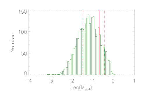
Figure 9: Properties of Eddington ratio of SDSS J1039. Histogram shows the Eddington ratio distributions of the 2872 SDSS quasars from Shen et al. (2011). Vertical solid red line marks the position $M_{\rm Edd}=0.216$, and vertical dashed red lines mark positions $M_{\rm Edd}=0.216\pm 0.179$.

Meanwhile, based on the estimated minimum and maximum BH masses of SDSS J1039  through the $M_{\rm BH}-\sigma$ relations and the estimated bolometric luminosity above, the dimensionless Eddington ratio $M_{\rm Edd}$ can be applied to trace intrinsic accretion rate in the SDSS J1039  and estimated by

$$\begin{split}M_{\rm Edd}&=\frac{L_{\rm bol}}{1.4\times 10^{38}M_{\rm BH}/{\rm M_{\odot}}}\\ &\sim 0.216\pm 0.179\end{split}$$ (8)

. Then, we compare the Eddington ratio of SDSS J1039  and the normal SDSS quasars reported in Shen et al. (2011) in Fig. 9. The 2872 SDSS quasars ($z<0.33$) are collected from the sample in Shen et al. (2011) by three criteria, redshift less than 0.33, the measured continuum luminosity at least 10 times larger than the corresponding uncertainty and the measured BH mass at least 10 times larger than the corresponding uncertainty. The Eddington ratios of the 2872 SDSS quasars are calculated by the same equation above. It is clear that the estimated Eddington ratio of SDSS J1039  is a common value among normal SDSS quasars.

The central AGN activities of SDSS J1039  are discussed above through the parameters of the continuum luminosity ${\rm 2.89\times 10^{42}erg~{}s^{-1}}$ (or bolometric luminosity $3.9\times 10^{43}{\rm erg~{}s^{-1}}$), and the Eddington ratio around 0.216. In the case of SDSS J1039  as a candidate of true Type-2 AGN, not similar as the expected BLRs disappearance in most of candidates of true Type-2 AGN with expected quite lower continuum luminosity (and/or quite lower Eddington ratios) or with expected quite higher luminosities, the SDSS J1039  has normal continuum luminosity relative to the [O iii] line luminosity and normal Eddington ratio, indicating SDSS J1039  has unique properties among the reported true Type-2 AGN. And further efforts should be necessary to consider the loss of broad emission lines in the candidate of true Type-2 AGN SDSS J1039.

The results discussed above can be well applied to give the conclusion that the SDSS J1039  is a better candidate of true Type-2 AGN, however more further efforts in the near future are necessary to robustly confirm the conclusion. First and foremost, multi-epoch spectroscopic results are necessary to give further robust clues that SDSS J1039  is not a changing-look AGN at dim state, besides the results shown in Fig. 7 on properties of continuum luminosity and total [O iii] luminosity. Besides, multi-band observation results are necessary to give more accurate estimation of bolometric luminosity. Unfortunately, in the current stage, there are only photometric data points in optical band and near infrared band for SDSS J1039. Therefore, the bolometric correction is roughly applied in the manuscript. Last but not the least, independent method is necessary to be applied to measure central BH mass of SDSS J1039, in order to find more accurate Eddington ratio.

It is clear that the SDSS J1039  can be well confirmed as a better candidate of true Type-2 AGN but with unique properties among the reported true Type-2 AGN, especially its natural luminosity and natural Eddington ratio as normal quasars. The results probably indicate that some unique AGN with disappearance of central BLRs are not due to particular properties of central accretion processes but could be be treated as a subclass of Type-1 AGN at special evolution stages. In the near future, some more true Type-2 AGN like SDSS J1039  could provide further clues on the nature of true Type-2 AGN.

Before the end of the section, simple discussions are listed on the pros and cons of the method to detect candidates of true Type-2 AGN by features of the lack of broad emission lines combining with the apparent long-term variability as what have been applied in the manuscript. The pros are as follows. First, the method applied in the manuscript is convenient to be applied to detect candidates of True Type-2 AGN among the large sample of narrow emission line galaxies in SDSS, combining with public light curves from CSS (Drake et al., 2009), ASAS-SN (All-Sky Automated Survey for Supernovae, http://www.astronomy.ohio-state.edu/asassn/index.shtml) (Shappee et al., 2014; Kochanek et al., 2017), ZTF (Zwicky Transient Facility, https://www.ztf.caltech.edu/) (Bellm et al., 2019; Masci et al., 2019), etc. Second, the method will lead to find more candidates of true Type-2 AGN with similar properties as those of normal broad line AGN, such as the SDSS J1039  reported in the manuscript, which could provide further considerations on physical nature of true Type-2 AGN. Third, the method mainly focuses on spectroscopic emission line features and long-term variability properties, leading to conveniently detect candidates of true Type-2 AGN at high redshift. Certainly, there are cons as follows. First, the final results also depend on quality of spectrum. High quality spectrum should lead to different conclusion, such as the more recent results in NGC3147 with detected broad lines in high quality HST spectrum. Second, lack of multi-band properties of spectral energy distributions will lead to estimated bolometric luminosity and Eddington ratio not accurate enough. Third, the method sensitively depends on apparent long-term variability properties, leading to miss candidates of true Type-2 AGN with unapparent variability.

4 Conclusions

Finally, we give our main conclusions as follows.

• Based on the high quality spectroscopic properties of SDSS J1039, a power law continuum component is preferred with confidence level higher than 7sigma through the F-test technique, besides the commonly considered host galaxy contributions.

• Emission line fitting procedure provides robust evidence to support that there are no broad Balmer emission lines in SDSS J1039. The F-test technique can tell the confidence level only around 6% to support broad emission line components.

• The upper limits of broad H$\beta$ line flux can be well estimated, leading the EW of broad H$\beta$ to be smaller than 13.5Å  with 99% confidence level, indicating no intrinsic broad emission lines in the SDSS spectrum of SDSS J1039.

• Under the Virialization assumption to BLRs combining with the strong correlation between continuum luminosity and H$\alpha$ line luminosity, the expected broad H$\alpha$ (if there was) can be well re-constructed, indicating that the expected broad H$\alpha$ can not be overwhelmed by noises in the SDSS spectrum of SDSS J1039.

• The long-term photometric variability of SDSS J1039  can be well described by DRW process with determined timescale about $100{\rm days}$, similar as the variability of normal SDSS quasars, strongly supporting the central AGN activities.

• SDSS J1039  does follow the same dependence of continuum luminosity on total [O iii] line luminosity as normal broad line AGN, indicating that SDSS J1039  is not a changing-look AGN at dim state but a better candidate of true Type-2 AGN.

• SDSS J1039  has normal luminosity and Eddington ratio, not similar as the expected lower luminosities (lower accretion rates) or higher luminosities, indicating SDSS J1039  is an unique Type-2 AGN with lack of central BLRs.

References

- Ahumada et al. (2020) Ahumada, R.; Allende P.; Almeida, A.; et al., 2020, ApJS, 249, 3
- Andrae, Kim & Bailer-Jones (2013) Andrae, R., Kim, D. W., & Bailer-Jones, C. A. L., 2013, A&A, 554, 137
- Antonucci & Miller (1985) Antonucci, R. J.; Miller, J. S. 1985, ApJ, 297, 621
- Antouncci (1993) Antonucci, R., 1993, ARA&A, 31, 473
- Audibert et al. (2017) Audibert, A.; Riffel, R.; Sales, D. A.; Pastoriza, M. G.; Ruschel-Dutra, D., 2017, MNRAS, 464, 2139
- Avni (1976) Avni, Y., 1976, ApJ, 210, 642
- Bailer-Jones (2012) Bailer-Jones, C. A. L., 2012, A&A, 546, A89
- Baldassare et al. (2020) Baldassare, V. F.; Geha, M.; Greene, J., 2020, ApJ, 896, 10
- Baldwin et al. (1981) Baldwin, J. A.; Phillips, M. M.; Terlevich, R., 1981, PASP, 93, 5
- Barth et al. (2014) Barth, A. J.; Voevodkin, A.; Carson, D. J.; Wozniak, P., 2014, ApJ, 147, 12
- Batiste et al. (2017) Batiste, M.; Bentz, M. C.; Raimundo, S. I.; Vestergaard, M.; Onken, C. A., 2017, ApJL, 838, 10
- Baskin & Laor (2018) Baskin, A.; Laor, A., 2018, MNRAS, 474, 1907
- Bellm et al. (2019) Bellm, E. C.; Kulkarni, S. R.; Graham, M. J.; et al., 2019, PASP, 131, 018002
- Bentz et al. (2013) Bentz, M. C., et al., 2013, ApJ, 767, 149
- Bianchi et al. (2012) Bianchi S., et al., 2012, MNRAS, 426, 3225
- Bianchi et al. (2019) Bianchi, S.; Antonucci, R.; Capetti, A; et al., 2019, MNRAS Letter, 488, 1
- Brockwell & Davis (2002) Brockwell, P. J., & Davis, R. A. 2002, Introduction to Time Series and Forecasting (2nd ed.; New York: Springer)
- Bruzual & Charlot (2003) Bruzual, G.; Charlot, S. 2003, MNRAS, 344, 1000
- Cao (2010) Cao, X. W., 2010, ApJ, 724, 855
- Cappellari (2017) Cappellari, M., 2017, MNRAS, 466, 798
- Choi et al. (2014) Choi, Y.; Gibson, R. R.; Becker, A. C.; et al., 2014, ApJ, 782, 37
- Cid Fernandes et al. (2005) Cid Fernandes, R., Mateus, A., Sodre, L., Stasinska, G., Gomes, J. M., 2005, MNRAS, 358, 363
- Cid Fernandes et al. (2011) Cid Fernandes, R.; Stasinska, G.; Mateus, A.; et al., 2011, MNRAS, 413, 1687
- Czerny & Hryniewicz (2011) Czerny, B.; Hryniewicz, K., 2011, A&A, 525 L8
- Czerny et al. (2004) Czerny, B.; Rozanska, A.; Kuraszkiewicz, J., 2004, A&A, 428, 39
- De Cicco et al. (2020) De Cicco, D.; Bauer, F. E.; Paolillo, M.; et al., 2020, A&A in press, arXiv:2011.08860
- Drake et al. (2009) Drake, A. J.; Djorgovski, S. G.; Mahabal, A., et al., 2009, ApJ, 696, 870
- Duras et al. (2020) Duras, F.; Bongiorno, A.; Ricci, F.; et al., 2020, A&A, 636, 73
- Elitzur & Ho (2009) Elitzur, M.; Ho, L. C., 2009, ApJL, 701, 90
- Elitzur & Netzer (2016) Elitzur, M.; Netzer, H., 2016, MNRAS, 495, 585
- Ferrarese & Merritt (2000) Ferrarese, F.; Merritt, D., 2000, ApJL, 539, 9
- Foreman-Mackey et al. (2013) Foreman-Mackey, D.; Hogg, D. W.; Lang, D.; Goodman, J., 2016, PASP, 125, 306
- Gebhardt et al. (2000) Gebhardt, K., et al., 2000, ApJL, 539, 13
- Gezari et al. (2017) Gezari, S.; Hung, T.; Cenko, S. B.; et al., 2017, ApJ, 835, 144
- Greene & Ho (2005) Greene, J. E.; Ho, L. C., 2005, ApJ, 630, 122
- Groves et al. (2006) Groves, B.; Kewley, L.; Kauffmann, G.; Heckman, T., 2006, NewAR, 50, 743
- Ho & Kim (2014) Ho, L. C.; Kim, M.-J., 2014, ApJ, 789, 17
- Ichikawa et al. (2015) Ichikawa, K.; Packham, C.; Ramos A., C.; et al., 2015, ApJ, 803, 57
- Juneau et al. (2014) Juneau, S.; Bournaud, F.; Charlot, S.; et al., 2014, ApJ, 788, 88
- Kashino et al. (2017) Kashino, D.; Silverman, J. D.; Sanders, D.; et al., 2017, ApJ, 835, 88
- Kaspi et al. (2000) Kaspi, S.; Smith, P. S.; Netzer, H.; et al., 2000, ApJ, 533, 631
- Kauffmann et al. (2003) Kauffmann, G.; Heckman, T. M.; Tremonti, C.; et al., 2003, MNRAS, 346, 1055
- Kewley et al. (2001) Kewley, L. J.; Dopita, M. A.; Sutherland, R. S.; Heisler, C. A.; Trevena, J., 2001, ApJ, 556, 121
- Kewley et al. (2006) Kewley, L. J.; Groves, B.; Kauffmann, G.; Heckman, T., 2006, ApJ, 372, 961
- Kewley et al. (2019) Kewley, L. J.; Nicholls, D. C.; Sutherland, R. S., 2019, ARA&A, 57, 511
- Kelly et al. (2009) Kelly, B. C.; Bechtold, J.; Siemiginowska, A., 2009, ApJ, 698, 895
- Kelly et al. (2014) Kelly, B. C.; Becker, A. C.; Sobolewska, M.; Siemiginowska, A.; Uttley, P., 2014, ApJ, 788, 33
- Kim et al. (2011) Kim, D.; Protopapas, P.; Byun, Y.; Alcock, C.; Khardon, R.; Trichas, M, 2011, ApJ, 735, 68
- Kormendy & Ho (2013) Kormendy, J.; Ho, L. C., 2013, ARA&A, 51, 511
- Kozlowski et al. (2010) Kozlowski, S.; Kochanek, C. S.; Udalski, A.; et al., 2020, ApJ, 708, 927
- Kochanek et al. (2017) Kochanek, C. S.; Shappee, B. J.; Stanek, K. Z.; et al., 2017, PASP, 129, 4502
- LaMassa et al. (2015) LaMassa, S. M., Cales, S., Moran, E. C., et al. 2015, ApJ, 800, 144
- Li et al. (2015) Li, Y.; Yuan, W.; Zhou, H. Y.; Komossa, S.; Ai, Y. L.; Liu, W. J.; Boisvert, J. H., 2015, AJ, 149, 75
- MacLeod et al. (2010) MacLeod, C. L.; Ivezic, Z.; Kochanek, C. S.; et al., 2010, ApJ, 721, 1014
- MacLeod et al. (2011) MacLeod, C. L.; Brooks, K.; Ivezic, z.; et al., 2011, ApJ, 728, 26
- MacLeod et al. (2016) MacLeod, C. L.; Ross, N. P.; Lawrence, A.; et al., 2016, MNRAS, 457, 389
- Madejski & Sikora (2016) Madejski, G.; Sikora, M., 2016, ARA&A, 54, 725
- Masci et al. (2019) Masci, F. J.; Laher, R. R.; Rusholme, B.; et al., 2019, PASP, 131, 018003
- McConnell & Ma (2013) McConnell, N. J.; Ma, C. P., 2013, ApJ, 764, 184
- McElroy et al. (2016) McElroy, R. E.; Husemann, B.; Croom, S. M.; et al., 2016, A&A Letter, 593, 8
- Nagao et al. (2004) Nagao, T.; Kawabata, K. S.; Murayama, T.; Ohyama, Y.; Taniguchi, Y.; Sumiya, R.; Sasaki, S. S., 2004, AJ, 128, 109
- Netzer (2015) Netzer, H., 2015, ARA&A, 53, 365
- Netzer (2020) Netzer, H., 2020, MNRAS, 488, 5185
- Nicastro et al. (2003) Nicastro, F., Martocchia, A., Matt, G., 2003, ApJ, 589, L13
- Osterbrock (1991) Osterbrock, D. E., 1991, PASP, 103, 874
- Peterson et al. (2004) Peterson, B. M., et al., 2004, ApJ, 613, 682
- Pons & Watson (2016) Pons, E.; Watson, M. G., 2016, A&A, 594, 72
- Rafiee & Hall (2011) Rafiee, A.; Hall, P. B., 2011, ApJS, 194, 42
- Rees (1984) Rees, M. J., 1984, ARA&A, 22, 471
- Richards et al. (2006) Richards, G. T.; Lacy, M.; Storrie-Lombardi, L. J.; et al., 2006, ApJS, 166, 470
- Ross et al. (2018) Ross, N. P.; Ford, K. E. S.; Graham, M., et al., 2018, MNRAS, 480, 4468
- Sanchez-Saez et al. (2019) Sanchez-Saez, P.; Lira, P.; Cartier, R.; et al., 2019, ApJS, 242, 10
- Savic et al. (2018) Savic, D.; Goosmann, R.; Popovic, L. C.; Marin, F.; Afanasiev, V. L., 2018, A&A, 614, 120
- Savorgnan & Graham (2015) Savorgnan, G. A. D.; Graham, A. W., 2015, MNRAS, 446, 2330
- Shappee et al. (2014) Shappee, B. J.; Prieto, J. L.; Grupe, D., et al., 2014, ApJ, 788, 48
- Shen et al. (2011) Shen, Y.; Richards, G. T.; Strauss, M. A; et al., 2011, ApJS, 194, 45
- Shi et al. (2010) Shi, Y.; Rieke, G. H.; Smith, P.; et al., 2010, ApJ, 714, 115
- Shimasaku et al. (2001) Shimasaku, K.; Fukugita, M.; Doi, M., et al., 2001, AJ, 122, 1238
- Starkey et al. (2016) Starkey, D. A.; Horne, K.; Villforth, C., 2016, MNRAS, 456, 1960
- Storchi-Bergmann et al. (1993) Storchi-Bergmann, T.; Baldwin, J. A.; Wilson, A. S., 1993, ApJL, 410, 11
- Strateva et al. (2001) Strateva, I.; Ivezic, Z.; Knapp, G. R., et al., 2001, AJ, 122, 1861
- Sulentic et al. (2000) Sulentic, J. W.; Marziani, P.; Dultzin-Hacyan, D., 2000, ARA&A, 38, 521
- Tie et al. (2017) Tie, S. S.; Martini, P.; Mudd, D.; et al., 2017, ApJ, 153, 107
- Tohline & Osterbrock (1976) Tohline, J. E., Osterbrock, D. E. 1976, ApJL, 210, L117
- Tran (2001) Tran, H. D., 2001, ApJL, 554, 19
- Tran (2003) Tran, H. D., 2003, ApJ, 583, 632
- Ulrich et al. (1997) Ulrich, M. H.; Maraschi, L.; Urry, C. M., 1997, ARA&A, 35, 445
- Woo et al. (2013) Woo, J.-H., et al., 2013, ApJ, 772, 49
- Woo et al. (2015) Woo, J.-H.; Yoon, Y.; Park, S.; Park, D.; Kim, S. C., 2015, ApJ, 801, 38
- Yang et al. (2018) Yang, Q.; Wu, X.; Fan, X.; et a;., 2018, ApJ, 862, 109
- Zaw et al. (2019) Zaw, I.; Chen, Y.; Farrar, G. R., 2019, ApJ, 872, 134
- Zhang (2014) Zhang, X. G., 2014, MNRAS, 438, 557
- Zhang & Feng (2017a) Zhang, X. G., Feng, L. L., 2017a, MNRAS, 464, 2203
- Zhang & Feng (2017) Zhang, X. G., Feng, L. L., 2017, MNRAS, 468, 620
- Zhang et al. (2019) Zhang, X. G.,; Bao, M., Yuan, Q. R., 2019, MNRAS Letter, 490, 81
- Zhang et al. (2020) Zhang, X. G., Feng, Y. Q., Chen, H., Yuan, Q. R., 2020, ApJ, 905, 97
- Zhang (2021a) Zhang, X. G., 2021a, ApJ, 909, 16, ArXiv:2101.02465
- Zhang (2021b) Zhang, X. G., 2021b, ApJ accepted, ArXiv:2107.09214
- Zu et al. (2011) Zu, Y.; Kochanek, C.S.; Peterson, B.M. 2011, ApJ, 735, 80
- Zu et al. (2013) Zu, Y.; Kochanek, C. S.; Kozlowski, S.; Udalski, A., 2013, ApJ, 765, 106
- Zu et al. (2016) Zu, Y.; Kochanek, C. S.; Kozlowski, S.; Peterson, B. M., 2016, ApJ, 819, 122