Quantum reference frames: derivation of perspective-dependent descriptions via a perspective-neutral structure

Abstract

In standard quantum mechanics, reference frames are treated as abstract entities. We can think of them as idealized, infinite-mass subsystems which decouple from the rest of the system. In nature, however, all reference frames are realized through finite-mass systems that are subject to the laws of quantum mechanics and must be included in the dynamical evolution. A fundamental physical theory should take this fact seriously. In this paper, we further develop a symmetry-inspired approach to describe physics from the perspective of quantum reference frames. We find a unifying framework allowing us to systematically derive a broad class of perspective dependent descriptions and the transformations between them. Working with a translational-invariant toy model of three free particles, we discover that the introduction of relative coordinates leads to a Hamiltonian structure with two non-commuting constraints. This structure can be said to contain all observer-perspectives at once, while the redundancies prevent an immediate operational interpretation. We show that the operationally meaningful perspective dependent descriptions are given by Darboux coordinates on the constraint surface and that reference frame transformations correspond to reparametrizations of the constraint surface. We conclude by constructing a quantum perspective neutral structure, via which we can derive and change perspective dependent descriptions without referring to the classical theory. In addition to the physical findings, this work illuminates the interrelation of first and second class constrained systems and their respective quantization procedures.

1 Introduction

1.1 On quantum reference frames

In this work, we follow the paradigm that the properties of physical systems $S$ have no absolute meaning but are only defined relatively to some other content of the universe. In theoretical classical mechanics and special relativity the role of this ”other content of the universe” is usually played by abstract frames of reference. As we treat these frames as external entities, they must be non-dynamical and sufficiently decoupled from $S$. Upholding the paradigm, let us think of reference frames as abstractions of physical systems, for example ideal rigid bodies with imprinted rulers defining orientations and distances. For such reference frames to not be affected by $S$, their mass must be much larger than that of $S$, at best infinite.

Of course, in reality, all reference frames are realised by finite-mass systems, for example some measurement devices in a laboratory. A fundamental approach should take the fact seriously that those real reference frames are subject to the laws of physics. This means that we cannot simply conjure up new frames, like we do in Galilean or Lorentz transformations. Instead, all reference frames must already be explicitly included in the dynamical evolution. Following this line of thought, reference frame transformations can be naively understood as ”jumping” between distinct parts of our system.

The conviction that meaningful physical statements can only be made about the relation between things and not about the relation between things and abstract space is at the core of Mach’s principle. According to one of the many circulating versions of this conjecture, Mach suggests that ”Local inertial frames are affected by the cosmic motion and distribution of matter” [1]. Historically, some effort was made to construct purely relational mechanics in line with Mach’s principle. Two exemplary Machian frameworks can be found in [2] and [3].

As a second paradigm, we assume the universal validity of quantum mechanics. Now, if reference frames are realised through physical systems they must also be subject to the laws of quantum theory (see [6]). One can for instance imagine transforming to another laboratory being in superposition to or entangled with the present one. In accepting both paradigms, we need to face the question of how to describe physics from the perspective of quantum reference frames (QRFs) and how to relate between such descriptions.

QRFs have been extensively discussed in literature, with the greatest share of papers examining topics in quantum information and in finite dimensional Hilbert spaces [7, 8, 9, 10, 11, 12, 13, 14, 15, 16, 17]. The main focus lies here on operational aspects of QRFs, such as how to communicate quantum information without a shared frame of reference. In [18, 19, 20] the relation of QRFs to superselection rules is discussed. Finally, the role of QRFs in infinite-dimensional Hilbert spaces and in the context of quantum foundations is investigated [21, 22, 23, 24, 25].

1.2 On perspective neutral structures

Our departing point is the paper ”Quantum mechanics and the covariance of physical laws in quantum reference frames” [24]. Giacomini, Castro-Ruiz and Brukner derived the transformations between reference frames attached to quantum particles without referring to an absolute background. It is shown that there is no unique way of defining such a transformation but that its form depends on a choice of preferred coordinates. The findings shine light on what a theory of ”quantum general covariance” could look like, a notion relevant in the context of quantum gravity.

The paper ”A change of perspective: switching quantum reference frames via a perspective-neutral framework” [25] aims to rederive the outcomes of [24] from first principles, embedding them in a structure better suited for generalization. Inspired from general relativity and quantum gravity the mathematical framework of constrained Hamiltonian systems is applied. The starting point is a Lagrangian with translational invariance. The Legendre-transformation of this Lagrangian fails to be surjective, resulting in a Hamilton theory which features a constraint of the total momentum and contains redundant variables. The resulting structure is thus interpreted as an observer-independent meta-theory which contains, so to say, all perspectives at once but is void of direct operational meaning.

Operationally meaningful observer-dependent descriptions can then be obtained by fixing the redundancies, which classically amounts to a choice of gauge. It is shown that canonical transformations between two observer-dependent descriptions can be understood as gauge-transformations. To obtain the associated quantum picture the authors follow two distinct paths. In the reduced quantization, the authors fix the redundancies classically before quantizing the system. This yields the quantum physics as seen from a specific observer. In the Dirac quantization it is the other way around: One quantizes first, then fixes the redundancies by a projection on the constraint-eigenstates. This leads to a perspective-neutral quantum theory. Vanrietvelde et al. show that one can re-obtain the lot of observer-dependent descriptions by unitarily rotating the system prior to projecting such that the constraint acts only on a selected degree of freedom.

In the opinion of the present author the approach introduced in [25] has one major downside: the unsymmetrical treatment of positions and momenta. While the theory features a constraint for the total momentum, there is none for the center-of-mass. A consequence of this privileged role of the momenta is that only a fraction of all perspective dependent descriptions can be obtained. Likewise, only the reference-frame transformations switching between those frames, constituting only a small subset of all possible canonical transformations, can be derived. How to embed the remaining ones is left unclear.

1.3 Summary of results

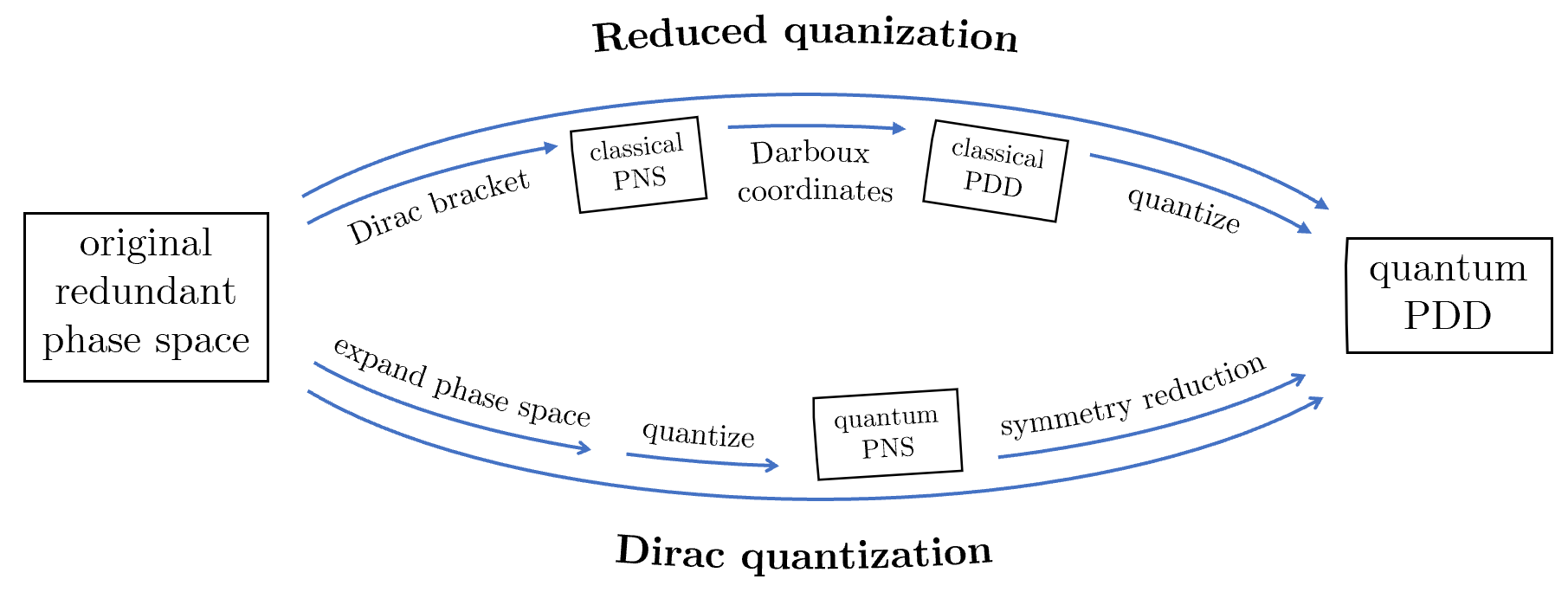
Figure 1: A schematic summary of the reduced and the Dirac quantization scheme. Here, PNS stands for ”perspective-neutral structure” and PDD for ”perspective-dependent description”.

In this article, we aim to address the identified shortcomings of [25]. We will discover that the theory created by Vanrietvelde et al. can be understood as part of a richer, more symmetrical framework where the positions and momenta are treated on equal footing. The resulting theory allows to uncover a broader set of perspective dependent frames, some of which were concealed in the original approach. Furthermore, we will systematically obtain the transformations connecting the perspective dependent frames, both in the classical and in the quantum picture. We will thus be able to derive additional transformations discussed in [24] from first principles. Besides those merits, in our extended framework, all appearing (relative) variables will be equipped with a clear physical meaning relating them to the description of an idealized outside observer. This will render the theory more accessible and further lead to a reinterpretation of some of the variables appearing in the original theory. It should be emphasized that the physics underlying the framework of the present article are equal to those of the original theory by Vanrietvelde et al., as both theories start from the same Lagrangian. We therefore expect to partly re-derive the results of [25].

The approach proposed in this article starts with a transformation to relative coordinates. This leaves us only with gauge-independent coordinates and eliminates all references to a Newtonian background already at the Lagrangian level. The associated Hamiltonian theory is more symmetrical and features two constraints for both relative positions and momenta. Unfortunately, the constraints do not commute, thus preventing direct quantization. We tackle this difficulty following two paths.

At first, we employ the reduced quantization scheme. Here we make use of the so-called Dirac-bracket, which can be understood as the Poisson bracket restricted to the constraint surface. Its core advantage is that the constraints Dirac-commute, paving the way for quantization. However, this comes at a price: We will see that the Dirac bracket is not of canonical form, i.e. that phase space coordinates referring to different particles do not commute along the constraint surface in general. In the style of Vanrietvelde et al. we interpret the set of Dirac-commuting, redundant coordinates as the classical perspective-neutral structure.

It can then be shown that the correct observer-dependent descriptions are given by those intrinsic coordinates of the constraint surface, whose Dirac bracket satisfies the canonical commutation relations. We will focus on two such descriptions: In the relative position frame two selected position coordinates match those seen from an external infinite mass-observer. In the relative momentum frame this holds for two momentum coordinates. While the former is included in [25], the latter is a new feature of the theory. The relative frames can now easily be quantized via the standard recipe. But since the quantization takes place only after having resolved the redundancies one cannot obtain a full quantum perspective neutral structure via the reduced quantization scheme.

To fix this, we follow a second path: We further expand the phase space and modify the constraints to make them commute. It will be shown that partially gauge fixing this extended space leaves us with a class of symplectomorphic auxiliary spaces. One of them is identical to the perspective-neutral structure found by Vanrietvelde et al., thus proving that the original theory is fully embedded in our new framework. However, the physical interpretation of the appearing relative variables must change. There appears to be evidence that only one of the many possible gauge fixes is physically meaningful. Thus, the gauge freedom will be replaced by the freedom to choose a set of darboux coordiantes. Quantizing the extended structure then yields the sought-after quantum perspective-neutral structure.

To re-obtain the perspective-dependent quantum descriptions we carry out a quantum symmetry reduction. It consists of two unitary transformations, each followed by a projection on either constraint. We will discover that with the first unitary we decide between relative position and relative momentum description, while the second unitary determines which particle will serve as the reference frame. Finally, we will see how the quantum perspective neutral structure can be employed to change between quantum reference frames. Figure 1 shows the connections between the various structures in a simplified scheme.

2 Classical Theory

2.1 Mathematical preliminaries: constrained Hamiltonian systems

In this section we will compactly review the mathematical formalism of constrained Hamiltonian systems, following largely [26]. The well-informed reader may skip this part.

2.1.1 Constraints through the Legendre transformation

Let us write the Euler-Lagrange-equations for a given Lagrangian $L$ in their expanded form

$$\ddot{q}_{n^{\prime}}J_{n^{\prime}n}=\frac{\partial L}{\partial q_{n}}-\dot{q}_{n^{\prime}}\frac{\partial^{2}L}{\partial q_{n^{\prime}}\partial\dot{q}_{n}},$$ (1)

where

$$J_{n^{\prime}n}=\frac{\partial^{2}L}{\partial\dot{q}_{n^{\prime}}\partial\dot{q}_{n}}.$$ (2)

We observe that this linear equation determines the accelerations $\ddot{q}_{n}$ uniquely only when the Jacobian is invertible, that is when the determinant

$$det\left(\frac{\partial^{2}L}{\partial\dot{q}_{n^{\prime}}\partial\dot{q}_{n}}\right)$$ (3)

does not vanish. This translates directly into the Hamilton formalism since $J_{n^{\prime}n}$ can be written as

$$J_{n^{\prime}n}=\frac{\partial p_{n^{\prime}}}{\partial q_{n}}.$$ (4)

We see that the non-vanishing of the determinant 3 is the condition for the invertibility of the velocities as function of the coordinates and momenta.

If the rank of $J_{n^{\prime}n}$ is equal to $N-M$ then the Legendre-transformation maps onto a $N-M$-dimensional submanifold of the phase-space. Only configurations contained in this subspace are physically meaningful. The constraint surface can be described by $M$ constraints

$$\varphi_{m}(q,p)\simeq 0,\quad m=1...M.$$ (5)

We have introduced the weak equality symbol $\simeq$ to emphasize that the quantity $\varphi_{m}$ is numerically restricted to be zero, but does not vanish throughout phase space [26]. This means that the derivatives of $\varphi_{m}$ do not vanish on the constraint surface in general. Therefore, the $\varphi$’s have in general nonzero Poisson brackets with other phase-space functions or the canonical coordinates and we must be cautious not to solve the constraints before calculating the Poisson brackets. An equation that holds everywhere in phase-space is called strong and will be denoted by the regular equality sign ”$=$”.

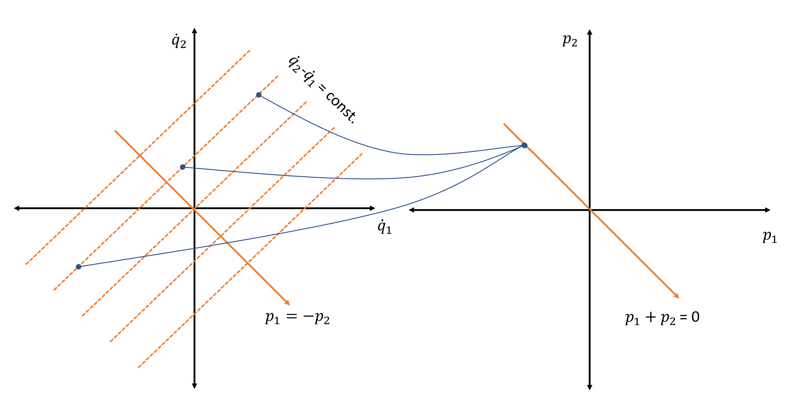
Figure 2: Illustration of the relation between velocities and momenta in a constrained system. The figure shows the Legendre transformation of a 2-dimensional system with the Lagrangian $L=1/2(\dot{q}_{1}-\dot{q}_{2})^{2}$. The momenta are $p_{1}=\dot{q}_{1}-\dot{q}_{2}$ and $p_{2}=\dot{q}_{2}-\dot{q}_{1}$. Since $p_{1}=-p_{2}$ the tuple $(p_{1},p_{2})$ describes only a 1-dimensional subspace of the $(\dot{q}_{1},\dot{q}_{2})$-space and all the $\dot{q}$’s on the line $\dot{q}_{2}-\dot{q}_{1}=c$ are mapped on the same point $p_{2}=-p_{1}=c$. We thus need additional parameters $y_{m}(q,\dot{q})$ to render the transformation invertible.

In the presence of constraints the variations $\delta q_{n}$ and $\delta p_{n}$ are no longer independent as we only allow for variations that are tangent to the constraint surface. We can equally state that all linear combinations of constraint variations must be weakly zero, i.e.

$$y_{m}\delta\varphi_{m}=y_{m}\frac{\partial\varphi_{m}}{\partial p_{n}}\delta p_{n}+y_{m}\frac{\partial\varphi_{m}}{\partial q_{n}}\delta q_{n}\simeq 0.$$ (6)

Comparing this equation with

$$\left(\frac{\partial H}{\partial q_{n}}+\frac{\partial L}{\partial q_{n}}\right)\delta q_{n}+\left(\frac{\partial H}{\partial p_{n}}-\dot{q}_{n}\right)\delta p_{n}=0.$$ (7)

and making use of the Euler-Lagrange equations leads to the Hamilton equation of motion for a constrained system

$$\begin{split}\dot{q}_{n}&=\frac{\partial H}{\partial p_{n}}+y_{m}\frac{\partial\varphi_{m}}{\partial p_{n}}=\frac{\partial H_{T}}{\partial p_{n}}\\ \dot{p}_{n}&=-\frac{\partial H}{\partial q_{n}}-y_{m}\frac{\partial\varphi_{m}}{\partial q_{n}}=\frac{\partial H_{T}}{\partial q_{n}}.\end{split}$$ (8)

Here we have introduced the total Hamiltonian

$$H_{T}=H(q,p)+y_{m}(q,p,t)\varphi_{m}(q,p)$$ (9)

as the original Hamiltonian plus linear combinations of the constraints.

$H_{T}$ is only well defined on the physical constraint surface and can be extended arbitrarily in the extended space. Choosing a specific extension corresponds to choosing the free auxiliary parameters $y_{m}$. As all physically sensible configurations must lie on the constraint surface, this extension does not change their respective energy values.

With the total Hamiltonian we can write the total time derivative of any function as

$$\begin{split}\dot{F}(q,p)&=[F,H_{T}]=[F,H]+[F,y_{m}\varphi_{m}]\\ &=[F,H]+[F,y_{m}]\varphi_{i}+y_{m}[F,\varphi_{m}]\\ &\simeq[F,H]+y_{m}[F,\varphi_{m}].\end{split}$$ (10)

2.1.2 Computing the consistency conditions

Consistency requires that the constraints be preserved in time, i.e that their total time derivative vanishes on the constraint surface. So plugging them into equation 10 gives rise to the consistency conditions

$$\begin{split}\dot{\varphi}_{m}=[\varphi_{m},H]+y_{m^{\prime}}[\varphi_{m},\varphi_{m^{\prime}}]\simeq 0,\end{split}$$ (11)

with

$$m,m^{\prime}=1,\dotso,M.$$ (12)

These equations reduce to one of the following three types [27]:

• If $\varphi_{m}$ commutes with all $\varphi_{m^{\prime}}$ but not with $H$, we obtain a relation of the form $\varphi_{k}(p,q)\simeq 0$. If linearly independent of the former constraints, this relation consitutes a further constraint on the system. It is evident that this new constraint must be conserved as well, leading to a new consistency condition and so forth. The cycle continues until we reach one of the stops below.

• If $\varphi_{m}$ does not commute with at least one constraint, we do not obtain a new constraint but a relation for the $y$’s.

• The equation reduces to either $0=0$ or $1=0$. The first case is automatically satisfied and leads to no further constraint, while the second one points to an inconsistency in the equations of motions. Such theories start from self-contradictory Lagrangians and are of no interest.

Having exhausted all equations we are left with a complete set of $J$ constraints. We can add them to the total Hamiltonian and let the consistency conditions run now over all constraints

$$[\varphi_{j},H]+y_{j^{\prime}}[\varphi_{j},\varphi_{j^{\prime}}]\simeq 0,\quad j,j^{\prime}=1,\dotso,J.$$ (13)

This set of linear equation is over-complete, since a part of it has already been solved to derive the secondary constraints. We see that the solutions depend crucially on the matrix of commutators

$$\Delta_{jj^{\prime}}=[\varphi_{j},\varphi_{j^{\prime}}].$$ (14)

If it is invertible then we can find unique solutions for all $y_{j}$ and thus the Hamiltonian and the time evolution of the system is unique too. If, however, $\Delta_{jj^{\prime}}$ has a vanishing determinant, then there are some zero eigenvectors and not all $y_{m}$ are uniquely determined.

Let us quickly introduce some new terminology. In [28], Dirac referred to any function on phase-space as first class, whose Poisson bracket with every constraint is weakly equal zero

$$[F,\varphi_{j}]\simeq 0\quad j=1...J.$$ (15)

The Hamiltonian, for example, is first class by design. A function which has at least one non-vanishing Poisson bracket with any constraint is called second class.

We now perform linear transformations $\varphi_{j}\rightarrow a_{jj^{\prime}}\varphi_{j^{\prime}}$ on the constraints. Our aim is to split the such transformed constraints into a subset $\gamma_{\alpha}$ of first class constraints and a subset $\Phi_{\alpha}$ of second class constraints. As combinations of weakly vanishing quantities also vanish weakly, the linear transformation does not change the theory. After having successfully carried out the transformation we can write the matrix of commutators in the form

$$\Delta=\begin{pmatrix}[\gamma_{a},\gamma_{b}]&[\Phi_{\alpha},\gamma_{b}]\\[4.0pt] [\gamma_{a},\Phi_{\beta}]&[\Phi_{\alpha},\Phi_{\beta}]\end{pmatrix}=\begin{pmatrix}0&0\\ 0&C_{\alpha\beta}\end{pmatrix}$$ (16)

The first class constraints $\gamma_{a}$ do not impose any condition on their respective $y_{a}$, which means that $y_{a}$ are arbitrary functions of the phase-space coordinates and time. The second class constraints $\Phi_{\alpha}$, on the contrary, have well defined $y_{\alpha}$, which we can compute by means of the equations 13. Finally we can write our new total Hamiltonian as the sum of the original Hamiltonian plus linear combinations of all constraints

$$\begin{split}H_{T}&=H+y_{\alpha}\Phi_{\alpha}+y_{a}(p,q,t)\gamma_{a}\\ &=H^{\prime}+y_{a}(p,q,t)\gamma_{a},\end{split}$$ (17)

where

$$H^{\prime}=H+y_{\alpha}\Phi_{\alpha}.$$ (18)

2.1.3 Gauge transformations by first-class constraints

Note that the above total Hamiltonian $H_{T}$ decomposes into two parts. While $H^{\prime}$, containing the original Hamiltonian plus the second-class constraints, generates a deterministic evolution, the contribution from $y_{a}(p,q,t)\gamma_{a}$ is completely arbitrary.

Let us take e.g. $f(q,p)=q$ and compute its value after an infinitesimal time span for distinct values of the $y_{a}$. We will obtain two different outcomes, their difference being

$$\Delta q(t_{0}+\delta t)=\delta t(y_{a}-y^{\prime}_{a})[q,\gamma_{a}].$$ (19)

As the time-dependence of the functions $y_{a}$ is not accessible, we have no means of saying anything about the evolution of $q$. This is of course incompatible with the deterministic character of classical mechanics. If we want unique solutions, it must be that operationally we cannot distinguish between two configurations $(q_{i},p_{i})$ and $(q^{\prime}_{i},p^{\prime}_{i})$ connected by a so-called gauge transformation

$$\begin{split}q_{i}\rightarrow q^{\prime}_{i}&=q_{i}+y_{a}[q_{i},\gamma_{a}]\\ p_{i}\rightarrow p^{\prime}_{i}&=p_{i}+y_{a}[p_{i},\gamma_{a}].\\ \end{split}$$ (20)

This means that even though a physical state is fully determined by the variables $(q,p)$, the converse is not true: A state does not uniquely determine a point in phase-space of $q$’s and $p$’s but a whole set of points. From equation 20 we learn that the gauge transformations connecting these points are generated by the first class constraints, which is in accordance with Noether’s theorem [29].

Furthermore, not all functions on phase-space correspond to physically measurable quantities. It is only the gauge invariant functions, that are those whose Poisson bracket with every first-class constraint vanishes weakly, which can be regarded as physically meaningful observables.

Second class constraints do not act as gauge generators, as they would map states out of the constraint surface. This can be seen by taking any second class constraint $\Phi_{\alpha}$ and checking the transformation induced by any other second class constraint $\Phi_{\beta}$

$$\Phi_{\alpha}\rightarrow\Phi_{\alpha}^{\prime}=\Phi_{\alpha}+\epsilon[\Phi_{\alpha},\Phi_{\beta}]\not\simeq 0.$$ (21)

2.2 Transformation to relative coordinates

In this section, we will work out the central structure of our paper, the second-class constrained Hamiltonian system. The departing point is a toy-model Lagrangian of three free particles in one dimension, reading

$$L(x,\dot{x})=\frac{1}{2}\sum_{i=1}^{3}m_{i}\dot{x}_{i}^{2}-\frac{M}{2}\dot{x}^{2}_{cm},$$ (22)

where

$$x_{cm}=(\sum_{i=1}^{3}m_{i}x_{i})/M$$

is the center-of-mass-position and

$$M=\sum_{i=1}^{3}m_{i}$$

the total mass of the system. By subtracting the center-of-mass kinetic energy we have rendered the Lagrangian invariant under local translations

$$(q_{i},\dot{q}_{i})\rightarrow(q_{i}+f(t),\dot{q}_{i}+\dot{f}(t))$$

where $f(t)$ is an arbitrary function of time. Because of this gauge symmetry the physical description depends only on relative degrees of freedom but not on the choice of external reference frame [25].

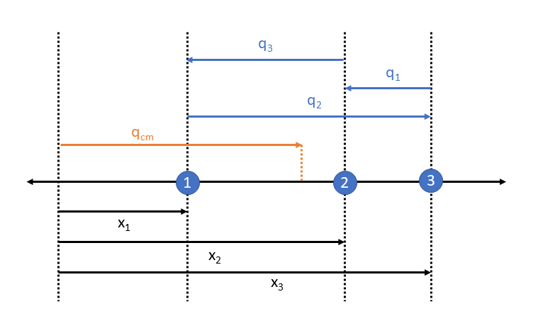
Figure 3: The figure shows the transformation 23 schematically. We notice that after the transformation $q_{cm}$ remains the only coordinate with respect to an external observer and that the $q_{i}$ are redundant.

The starting idea of this paper is to make the reference-frame independence explicit by going over to the coordinates

$$\begin{split}x_{1}-x_{2}&=q_{3}\\ x_{3}-x_{1}&=q_{2}\\ x_{2}-x_{3}&=q_{1}\\ \frac{1}{M}\sum_{i=1}^{3}m_{i}x_{i}&=q_{cm}.\end{split}$$ (23)

The three relative coordinates $q_{i}$ are invariant under local spatial translations, while the center-of-mass coordinate remains gauge dependent and still refers to the Newtonian background.

In geometrical terms the transformation 23 corresponds to a mapping from $\mathbb{R}^{3}$ into $\mathbb{R}^{4}$, reaching only points on the 3-dimensional hypersurface

$$q_{1}+q_{2}+q_{3}\equiv Q=0.$$ (24)

It follows that the $q_{i}$ are redundantly defined; we can always express one of the relative distances by means of the other two.

The Lagrangian 22 expressed in the new coordinates reads

$$L^{\prime}(q,\dot{q})=\frac{1}{2}\sum_{i=1}^{3}\mu_{i}\dot{q}_{i}^{2}+q_{4}(q_{1}+q_{2}+q_{3})$$ (25)

where we have introduced the quantities

$$\mu_{i}=\frac{m_{j}m_{k}}{M},\quad i\neq j\neq k,$$ (26)

which are called reduced masses and added the constraint $Q$ together with a Lagrange multiplier $q_{4}$. The calculation is given in appendix A.

Given only the Lagrangian 25, the role of $q_{4}$ as a Lagrange multiplier is not apparent. It follows that $q_{4}=q_{4}(t)$ can be treated as just another dynamical variable and that it enters the formalism on equal footing with the first three $q_{i}$ [31]. We observe that the Lagrangian, as expected, does not depend on the gauge-dependent center-of-position $q_{cm}$. This degree of freedom is of no physical relevance and will be discarded.

Let us now apply the methods established throughout section 2.1 to obtain the Hamilton theory. We start by computing the conjugate momenta

$$\begin{split}p_{i}&=\frac{\partial L}{\partial\dot{q}_{i}}=\mu_{i}\dot{q}_{i}\quad i=1,2,3\\ p_{4}&\simeq 0.\end{split}$$ (27)

There is one constraint $p_{4}\simeq 0$, which is added with yet another Lagrange multiplier $y_{i}$ to the standard Hamiltonian $H^{\prime}$ yielding

$$\begin{split}H&\simeq H^{\prime}(q,p)+y_{i}\Phi_{i}\\ &\simeq\sum_{i}p_{i}\dot{q}_{i}(q,p)-L(q,\dot{q}_{i}(q,p))+y_{i}\Phi_{i}\\ &\simeq\frac{1}{2}\sum_{i=1}^{3}\left(\frac{p_{i}^{2}}{\mu_{i}}-q_{4}q_{i}\right)+yp_{4}.\end{split}$$ (28)

Starting from Hamiltonian 28 we need to work through the consistency scheme discussed in section 2.1.2. The calculation, done in detail in appendix B, yields the Hamiltonian

$$H=\frac{1}{2}\sum_{i}\frac{p_{i}^{2}}{\mu_{i}}.$$ (29)

together with 2 effective constraints

$$\Phi_{1}=\sum_{i}q_{i},\quad\Phi_{2}=\sum_{i}\frac{p_{i}}{\mu_{i}}.$$ (30)

In the original phase-space $\mathcal{P}_{orig}\sim\mathbb{R}^{6}$, coordinatized by the $q_{i}$ and $p_{j}$, they define a 4-dimensional constraint surface $\Phi_{1}\simeq\Phi_{2}\simeq 0$, on which all physically sensible configurations must lie. Clearly, they are second-class as

$$[\Phi_{1},\Phi_{2}]=\sum_{i}\frac{1}{\mu_{i}}.$$ (31)

It can be shown that the structure 29 & 30 is symplectomorphic to the perspective neutral structure proposed in [25], i.e. to

$$H=\frac{1}{2}\sum_{i}\frac{\tilde{p}_{i}^{2}}{m_{i}},\quad\Phi_{1}=\sum_{i}\tilde{p}_{i},$$ (32)

if the latter is gauge fixed by

$$\tilde{\Phi}_{2}=\sum_{i}\mu_{i}x_{i}.$$ (33)

In the following sections, we will see that this choice of gauge is critical for the construction of our version of the perspective neutral structure which eventually leads to the derivation of further perspective-dependent descriptions. In fact, it is the critical difference between our work and [25], where the system was gauge-fixed by $q_{i}=0$. There, the gauge fix 33 must seem arbitrary as there is no reason to assume a preferred role for this specific observer. In our scheme, however, it becomes clear, that it is exactly 33 which gives meaning to the variables as relative coordinates. In other words: if one starts with relative variables, 33 arises as necessary consequence of the over-parametrization of the configuration space.

3 Reduced quantization of second class constraints

3.1 Mathematical preliminaries: Dirac bracket and Darboux coordinates

If there are no constraints present and the phase-space is linear there is a standard quantization recipe (see e.g. Dirac [32], p. 84ff). It tells us to assign to each function an operator acting on some Hilbert space $\mathcal{H}$ such that the commutator of quantum operators equals $i\hbar$ times the operator of the Poisson bracket

$$[\hat{F},\hat{G}]=i\hbar\widehat{[F,G]}.$$ (34)

In the presence of second-class constraints the quantization procedure is more involved. Classically, the constraints restrict the system to a submanifold of the original phase space. We would like to mirror this behaviour in the quantum theory by imposing the restrictions

$$\hat{\Phi}_{\alpha}\ket{\phi}_{phys}=0\quad\forall\;\alpha$$ (35)

on the state vectors $\ket{\phi}_{phys}$ which span the physical Hilbert space $\mathcal{H}_{phys}$. From the consecutive application of constraints $\hat{\Phi}_{\alpha}\hat{\Phi}_{\beta}\ket{\phi}_{phys}=0$ and $\hat{\Phi}_{\beta}\hat{\Phi}_{\alpha}\ket{\phi}_{phys}=0$ it follows readily that

$$[\hat{\Phi}_{\alpha},\hat{\Phi}_{\beta}]\ket{\phi}_{phys}=0.$$ (36)

The commutator of second class constraints however is not a constraint itself so that equation 36 is only satisfied when $\ket{\phi}_{phys}=0$. But then $\mathcal{H}_{phys}=\{0\}$ and the theory is trivial [33].

The difficulties originate already in the classical theory: While the constraints vanish on the constraint surface, their first derivatives in general do not, leaving the Poisson bracket ambiguous. This means, for a function $f$ on the phase space and a constraint $\Phi\simeq 0$ we have $f+\Phi\simeq f$, but in general

$$[f,g]\not\simeq[f+\Phi,g].$$ (37)

A solution to both the problems in classical and quantum theory was developed by P.A.M. Dirac in 1950 (see [27] and for a detailed derivation [28]). He generalized the original Poisson bracket to the Dirac bracket, given by

$$\{F,G\}=[F,G]-[F,\Phi_{\alpha}]C^{\alpha\beta}[\Phi_{\beta},G]$$ (38)

where $C^{\alpha\beta}$ is the inverse of the second-class bracket-matrix $C_{\alpha\beta}$ appearing in 16. The core advantage is that the Dirac bracket of an arbitrary function with any second class constraint vanishes:

$$\{\Phi_{\alpha},F\}=0.$$ (39)

From a geometrical viewpoint, the Dirac bracket is related to the pull-back of the symplectic two-form onto the constraints surface and picks up only those variations tangent to it [26]. As a consequence, there are in general always contributions from non-Poisson-commuting observables. This entails that Poisson-commuting observables are in general not Dirac-commuting. We will see this concretely in the next section.

By virtue of 39, the Dirac bracket, unlike the Poisson bracket, is unambiguous, i.e.

$$f^{\prime}\simeq f\rightarrow\{f^{\prime},\cdot\}\simeq\{f,\cdot\},$$

such that we can set the constraints to zero before computing the bracket. To quantize a second-class system, we simply replace the Poisson bracket by the Dirac Bracket in the correspondence rule

$$[\hat{F},\hat{G}]=i\hbar\widehat{\{F,G\}}.$$ (40)

The constraint operators can now be given any c-values, in particular $\Phi_{\alpha}=0$, enforcing the restriction 35. When we have found a representation of 40 we have found the quantum theory.

• This is a highly nontrivial problem which has no general solution. It can be solved only in special instances, for example when the Dirac bracket amounts to c-numbers. Luckily, this is exactly the case for our system at hand.

There is yet an alternative to trying to solve 40 directly. With the Dirac bracket, the second-class constraints can be treated as strong identities expressing some canonical coordinates in terms of others. This allows us to go over to intrinsic (local) coordinates $u_{i}(q,p),\pi_{i}(q,p),i=1,\dots,N-M$ spanning the constraint surface. Expressed in the new coordinates the constraints $\Phi_{\alpha}(q_{n}(u_{i},\pi_{i}),p_{n}(u_{i},\pi_{i}))$ vanish identically [34]. Of special interest are those intrinsic coordinates which Dirac-commute according to the canonical commutation relations

$$\{u_{i}(q,p),\pi_{j}(q,p)\} =\delta_{ij}$$ (41)

$$\{u_{i}(q,p),u_{j}(q,p)\} =\{\pi_{i}(q,p),\pi_{j}(q,p)\}=0.$$ (42)

They are referred to as Darboux coordinates [34]. When they are found, we have obtained a reduced theory, with no constraints present and no redundancies left. The Darboux coordinates are nicely canonical so that from this point on we can follow the standard quantization procedure to obtain the quantum theory.

• Darboux coordinates are only defined up to a canonical transformation, but canonical quantization and canonical transformations are generally non-commutative operations. They do commute only for linear and point transformations (in both $q$ and $p$) [35].

Last but not least it is worth noticing that the Dirac bracket with any first class constraint is weakly equal to the Poisson bracket. Thus the equations of motions remain invariant under the replacement

$$\dot{F}=\{F,H\}\simeq[F,H].$$ (43)

3.2 The classical perspective-neutral structure

We will now apply the reduced quantization scheme to our theory at hand. At first, let us compute the Dirac-bracket. The bracket-matrix 14 reads

$$C=\begin{pmatrix}0&\mu\\ -\mu&0\\ \end{pmatrix}$$ (44)

where we have introduced

$$\mu=\sum_{i}\frac{1}{\mu_{i}}.$$ (45)

Since either $C^{-1}$ or the Poisson bracket of coordinates and constraints vanish, most of the terms in 38 drop out and we obtain

$$\begin{split}\{q_{i},q_{j}\}&=0\\ \{p_{i},p_{j}\}&=0\\ \{q_{i},p_{j}\}&=\delta_{ij}-\frac{1}{\mu\mu_{i}}.\end{split}$$ (46)

In the style of Vanrietvelde et al. I now propose to interpret the Dirac bracket 46 along with the constraints 30 and the Hamiltonian 29 as the classical perspective-neutral structure, living in the 6-dimensional phase space $\mathcal{P}_{orig}.$ As all relative variables are treated on equal footing it contains all perspectives at once while the inherent redundancies prevent an immediate operational interpretation.

Note that position and momentum observables of different particles do not Dirac-commute. This follows from the fact, that the $q_{i}$’s and $p_{i}$’s form a redundant over-parametrization of the phase space. As we restrict to the constraint surface, a variation of one of the $q_{i}$’s ($p_{i}$’s, respectively) necessarily entails some variation of the other relative position or momentum coordinates.

This has the seemingly counter-intuitive consequence that the Dirac-bracket of two $q$’s and two $p$’s, naively chosen as intrinsic coordinates, does not fulfill the canonical commutation relations, i.e., that this choice of intrinsic coordinates is non-Darboux. In the quantum picture, the impossibility to find simultaneous eigenvectors of the $\hat{q}$’s and $\hat{p}$’s even for distinct particles follows. Therefore, from the perspective of one particle the Hilbert space of the two other particles can not be partitioned as $H_{i,j}=H_{i}\otimes H_{j}$ and the standard quantization recipe is bound to fail.

Thinking in physical terms, the commutation relations 46 mean that $q_{i}$ and $p_{j}$ cannot be measured simultaneously and that there exist uncertainty relations between those variables. But why should a position measurement of one particle affect the momentum of another unrelated particle? The solution to this alleged paradox lies again in the finite mass $m$ of the system serving as reference frame and has already been presented in [21, 22, 23]. It follows from the uncertainty principle that if one wants to measure the position of a particle with an accuracy $\Delta x$ a finite amount of momentum

$$\Delta p>\frac{\hbar}{\Delta x}$$ (47)

has to be exchanged. The system serving as reference frame is therefore boosted by an uncertain amount $\frac{\Delta p}{m}$. In classical mechanics one can always keep the amount of exchanged momentum arbitrary small, such that $\Delta p<<m$. In the quantum regime, however, this approximation is no longer valid as masses are small and $\Delta p$ increases with measurement accuracy. Here, one can always envisage a measurement where $\Delta p\sim m$, resulting in a non negligible kickback of the reference system [21].

Figure 4: The figure shows a naive choice of internal coordinates $(u_{i},\pi_{j})$ that do not Dirac-commute according to the canonical commutation relations. The position vectors $q_{i}$ on the left hand side live in the configuration space. Displayed on the right hand side are the momentum vectors $p_{j}$, living in momentum space.

Note that there is no configuration of the masses which reproduces the standard bracket structure for all three coordinate pairs. If, however, one of the particles masses is much larger than the others, this particle can serve as a classical reference frame. For example, for $m_{1}>>m_{2}\sim m_{3}$ the mass term $\frac{m_{i}}{M}=\frac{1}{\mu\mu_{i}}$ converges to zero and we re-obtain the canonical commutation relations. Further, $\mu_{1}\rightarrow 0$ and $\mu_{2}\rightarrow m_{3},\mu_{3}\rightarrow m_{2}$ such that the perspective-neutral Hamiltonian 29 converges to the standard Hamiltonian for a two-particle system. This is an important result. It shows that the standard way of describing physics from an infinite-mass frame is fully embedded in our newly developed framework.

3.3 Perspective-dependent frames

In the section above, we saw that not all sets of intrinsic coordinates are physically useful. Thus, if we want observer-dependent descriptions which can be canonically quantized for arbitrary mass configurations we must search for Darboux coordinates. To keep it simple and not encounter any mathematical pitfalls we restrict to those which are linear in the original positions and momenta and do not mix them. Their most general form is given by

$$\begin{split}\begin{pmatrix}q_{1}\\ q_{2}\\ q_{3}\end{pmatrix}=\begin{pmatrix}m_{1A}u_{A}+m_{1B}u_{B}\\ m_{2A}u_{A}+m_{2B}u_{B}\\ m_{3A}u_{A}+m_{3B}u_{B}\end{pmatrix}\\ \begin{pmatrix}p_{1}\\ p_{2}\\ p_{3}\end{pmatrix}=\begin{pmatrix}n_{1A}\pi_{A}+n_{1B}\pi_{B}\\ n_{2A}\pi_{A}+n_{2B}\pi_{B}\\ n_{3A}\pi_{A}+n_{3B}\pi_{B}\end{pmatrix}.\end{split}$$ (48)

The 12 coefficients must satisfy 4 constraints

$$\sum_{i}m_{iA} =0 \qquad\sum_{i}\frac{n_{iA}}{\mu_{i}} =0$$ (49)

$$\sum_{i}m_{iB} =0 \qquad\sum_{i}\frac{n_{iB}}{\mu_{i}} =0$$

as well as 9 Darboux conditions

$$m_{iA}n_{jA}+m_{iB}n_{jB}=\delta_{ij}-\frac{1}{\mu\mu_{i}}$$ (50)

with

$$i,j=1,2,3.$$ (51)

The Darboux conditions enforce the canonical commutation relations between the intrinsic coordinates. Of these 13 constraints only 8 are linearly independent, leaving us with 4 free coefficients.

Still, we are left with a plethora of possible descriptions. How do we choose among them? I propose to coordinatize the constraint surface by two of the $q_{i}$ or $p_{j}$ and then to complete the remaining coordinates according to 49 - 50. Following this line of thought, I want to lay emphasis on two internal descriptions. For $m_{1}\rightarrow\infty$ both of them will converge to the ”classical” description from an external infinite-mass frame.

3.3.1 The relative position frame

Let us choose $m_{2A}=-m_{3B}=1$ and $m_{2B}=m_{3A}=0$ and set the placeholders to $A=3,B=2$, such that the position coordinates are named according to figure 4. By applying the constraints and working through the Darboux conditions we arrive at

$$\begin{split}\begin{pmatrix}q_{1}\\ q_{2}\\ q_{3}\end{pmatrix}&=\begin{pmatrix}u_{2}-u_{3}\\ u_{3}\\ -u_{2}\end{pmatrix}\\ \begin{pmatrix}p_{1}\\[4.0pt] p_{2}\\[4.0pt] p_{3}\end{pmatrix}&=\frac{1}{\mu}\begin{pmatrix}(\frac{\pi_{2}}{\mu_{3}}-\frac{\pi_{3}}{\mu_{2}})\\[4.0pt] \frac{1}{\mu_{3}}\pi_{2}+(\mu-\frac{1}{\mu_{2}})\pi_{3}\\[4.0pt] -(\mu-\frac{1}{\mu_{3}})\pi_{2}-\frac{1}{\mu_{2}}\pi_{3}\end{pmatrix}.\end{split}$$ (52)

In this description we have a direct expression for the distances between particle 1 & 3 and 1 & 2, respectively, while the distance between 2 & 3 can only be indirectly computed through $u_{2}-u_{3}$. It seems therefore reasonable to interpret 52 as the physics seen from the perspective of particle 1. The internal position observables are in accordance with those seen from an external infinite-mass frame, while the internal momentum observables are linear combinations thereof. By such reasoning we name this set of variables the relative position frame of particle 1.

Plugging 52 into the perspective-neutral Hamiltonian 29 yields

$$H_{q1}=\frac{1}{2\mu}\Big{(}(\frac{\mu}{\mu_{3}}-\frac{1}{\mu_{3}^{2}})\pi_{2}^{2}+(\frac{\mu}{\mu_{2}}-\frac{1}{\mu_{2}^{2}})\pi_{3}^{2}+2\frac{\pi_{2}\pi_{3}}{\mu_{2}\mu_{3}}\Big{)}$$ (53)

which looks tidier when expressed in the original masses

$$H_{q1}=\frac{1}{2}\left(\frac{m_{1}+m_{2}}{m_{1}m_{2}}\pi_{2}^{2}+\frac{m_{1}+m_{3}}{m_{1}m_{3}}\pi_{3}^{2}+2\frac{\pi_{2}\pi_{3}}{m_{1}}\right).$$ (54)

The index q next to $H$ indicates that we are we are in the relative position representation and the 1 that we are using particle 1 as reference frame. Observe that apart from the potential energy, which we have assumed to be zero, our outcome is identical to the findings of [25]. The modification to other particles follows readily.

3.3.2 The relative momentum frame

Let us now choose $n_{2A}=-n_{3B}=1$ and $n_{2B}=n_{3A}=0$ and set the placeholders again to $A=3,B=2$, such that the momentum coordinates are named according to the right side of figure 4. In this setup we coordinatize the constraint surface by

$$\begin{split}\begin{pmatrix}q_{1}\\ q_{2}\\ q_{3}\end{pmatrix}&=\frac{1}{\mu}\begin{pmatrix}\frac{1}{\mu_{1}}(v_{3}-v_{2})\\ \frac{v_{2}}{\mu_{2}}+(\mu-\frac{1}{\mu_{2}})v_{3}\\ -(\mu-\frac{1}{\mu_{3}})v_{2}-\frac{v_{3}}{\mu_{3}}\end{pmatrix}\\ \begin{pmatrix}p_{1}\\ p_{2}\\ p_{3}\end{pmatrix}&=\begin{pmatrix}-\mu_{1}(\frac{\rho_{3}}{\mu_{2}}-\frac{\rho_{2}}{\mu_{3}})\\ \rho_{3}\\ -\rho_{2}.\end{pmatrix}\end{split}$$ (55)

Observe that now only the momenta of particle 2 & 3 correspond to the external view, while the remaining momentum and all positions are expressed through linear combinations of the $v$’s and $\rho$’s. We will call this set of internal observables the relative momentum frame of particle 1. In this frame the Hamiltonian reads

$$H_{p1}=\frac{1}{2}\Big{(}\frac{\mu_{1}+\mu_{2}}{\mu_{2}^{2}}\rho_{3}^{2}+\frac{\mu_{1}+\mu_{3}}{\mu_{3}^{2}}\rho_{2}^{2}-\frac{2\mu_{1}}{\mu_{2}\mu_{3}}\rho_{2}\rho_{3}\Big{)}.$$ (56)

The relative momentum frame cannot be derived directly via the framework of [25]. This shows that while encompassing its precursor’s finding, the approach proposed in this article shines further light on the theory of QRFs.

3.4 Changing quantum reference frames

Our next objective is to find the connection between canonical QRF-transformations and the perspective neutral structure. In contrast to the work of Vanrietvelde et al., in our framework, reference frame transformations cannot amount to gauge transformations, as there is no gauge-freedom in purely second-class systems. In exchange, we have the freedom to choose any Darboux-parametrization of the constraint surface, each of which is corresponding to a perspective dependent description. As all sets of Darboux coordinates are connected via a canonical transformation, we can conclude: To canonically transform between two perspective dependent descriptions means to Darboux-reparametrize the constraint surface.

Finding the (quantum) canonical transformation connecting two descriptions is a three-step-process:

1. We write the original, relative phase space variables $(q,p)$ in terms of the two sets of Darboux coordinates $(u_{j},\pi_{j})$ and $(\bar{u}_{j},\bar{\pi}_{j})$.

2. We use this embedding in the perspective neutral structure to find the expression of one set of coordinates in terms of the other, i.e.

   $$\bar{u}_{i} =a_{ij}u_{j}$$ (57)

   $$\bar{\pi}_{i} =b_{ij}\pi_{j}.$$

3. To obtain the transformation in the quantum picture we compute the unitary representation of the given canonical transformation, e.g. by the methods derived in [36] or by means of appendix C.

Let us make this procedure explicit in three examples, where we set $m_{i}=1$ for simplicity.

3.4.1 Relative position to relative position

If we want to compute the transformation between two relative position frame, for instance of particle 1 and 2, we write

$$\begin{split}\begin{pmatrix}q_{1}\\ q_{2}\\ q_{3}\end{pmatrix}&=\begin{pmatrix}u_{2}-u_{3}\\ u_{3}\\ -u_{2}\end{pmatrix}=\begin{pmatrix}-\bar{u}_{3}\\ \bar{u}_{3}-\bar{u}_{1}\\ \bar{u}_{1}\end{pmatrix}\\ \begin{pmatrix}p_{1}\\ p_{2}\\ p_{3}\end{pmatrix}&=\frac{1}{3}\begin{pmatrix}\pi_{2}-\pi_{3}\\ \pi_{2}+2\pi_{3}\\ -2\pi_{2}-\pi_{3}\end{pmatrix}=\frac{1}{3}\begin{pmatrix}-\bar{\pi}_{1}-2\bar{\pi}_{3}\\ -\bar{\pi}_{1}+\bar{\pi}_{3}\\ 2\bar{\pi}_{1}+\bar{\pi}_{3}\end{pmatrix}.\end{split}$$ (58)

From this we can read off the canonical transformation

$$u_{2} =-\bar{u}_{1}, \qquad u_{3} =\bar{u}_{3}-\bar{u}_{1}$$ (59)

$$\pi_{2} =-(\bar{\pi}_{1}+\bar{\pi}_{3}) \qquad\pi_{3} =\bar{\pi}_{3}.$$

Giacomini et.al [24] found that the transformation 59 can be represented by the unitary operator

$$H_{2}\otimes H_{3}\rightarrow H_{3}\otimes H_{1}$$ (60)

$$\hat{S}_{q1\rightarrow q2}=\hat{\mathcal{Q}}_{2,1}e^{i\hat{u}_{2}\hat{\pi}_{3}}$$

where $\hat{\mathcal{Q}}_{A,B}$ is the position parity-swap operator, acting on vectors in $H_{A}\otimes H_{B}$ as

$$\hat{\mathcal{Q}}_{A,B}\ket{x}_{A}\otimes\ket{\Psi}_{B}=\ket{\Psi}_{B}\otimes\ket{-x}_{C}.$$ (61)

3.4.2 Relative momentum to relative momentum

We write out the relative momentum representations of particle 1 and 2:

$$\begin{split}\begin{pmatrix}q_{1}\\ q_{2}\\ q_{3}\end{pmatrix}&=\frac{1}{3}\begin{pmatrix}u_{2}-u_{3}\\ u_{2}+2u_{3}\\ -2u_{2}-u_{3}\end{pmatrix}=\frac{1}{3}\begin{pmatrix}-\bar{u}_{1}-2\bar{u}_{3}\\ -\bar{u}_{1}+\bar{u}_{3}\\ 2\bar{u}_{1}+\bar{u}_{3}\end{pmatrix}\\ \begin{pmatrix}p_{1}\\ p_{2}\\ p_{3}\end{pmatrix}&=\begin{pmatrix}\pi_{2}-\pi_{3}\\ \pi_{3}\\ -\pi_{2}\end{pmatrix}=\begin{pmatrix}\bar{\pi}_{3}\\ \bar{\pi}_{3}-\bar{\pi}_{1}\\ \bar{\pi}_{1}\end{pmatrix}.\end{split}$$ (62)

Again, we read off the canonical transformation

$$u_{2} =-(\bar{u}_{1}+\bar{u}_{3}) \qquad u_{3} =\bar{u}_{3}$$ (63)

$$\pi_{2} =-\bar{\pi}_{1}, \qquad\pi_{3} =\bar{\pi}_{3}-\bar{\pi}_{1}.$$

and the associated unitary

$$H_{2}\otimes H_{3}\rightarrow H_{3}\otimes H_{1}$$ (64)

$$\hat{S}_{p1\rightarrow p2}=\hat{\mathcal{P}}_{2,1}e^{i\hat{\pi}_{2}\hat{u}_{3}}$$

where $\hat{\mathcal{P}}_{A,B}$ is now the momenta parity-swap operator, acting as

$$\hat{\mathcal{P}}_{A,B}\ket{p}_{A}\otimes\ket{\Psi}_{B}=\ket{\Psi}_{B}\otimes\ket{-p}_{C}.$$ (65)

3.4.3 Relative position to relative momentum

This time, we compute the transformation between the relative position and relative momentum of particle 1. We write

$$\begin{split}\begin{pmatrix}q_{1}\\ q_{2}\\ q_{3}\end{pmatrix}&=\begin{pmatrix}u_{2}-u_{3}\\ u_{3}\\ -u_{2}\end{pmatrix}=\frac{1}{3}\begin{pmatrix}\bar{u}_{2}-\bar{u}_{3}\\ \bar{u}_{2}+2\bar{u}_{3}\\ -2\bar{u}_{2}-\bar{u}_{3}\end{pmatrix}\\ \begin{pmatrix}p_{1}\\ p_{2}\\ p_{3}\end{pmatrix}&=\frac{1}{3}\begin{pmatrix}\pi_{2}-\pi_{3}\\ \pi_{2}+2\pi_{3}\\ -2\pi_{2}-\pi_{3}\end{pmatrix}=\begin{pmatrix}\bar{\pi}_{2}-\bar{\pi}_{3}\\ \bar{\pi}_{3}\\ -\bar{\pi}_{2}\end{pmatrix}\end{split}$$ (66)

Again, we read off the canonical transformation

$$u_{2} =\frac{1}{3}(2\bar{u}_{2}+\bar{u}_{3}) \qquad u_{3} =\frac{1}{3}(\bar{u}_{2}+2\bar{u}_{3})$$ (67)

$$\pi_{2} =2\bar{\pi}_{2}-\bar{\pi}_{3}, \qquad\pi_{3} =-\bar{\pi}_{2}+2\bar{\pi}_{3}$$

The associated unitary representation is

$$H_{1}\otimes H_{2}\rightarrow H_{1}\otimes H_{2}$$ (68)

$$\hat{S}_{q1\rightarrow p1}=e^{-i\frac{\log{3}}{2}(u_{2}-u_{3})(\pi_{2}-\pi_{3})},$$

see appendix C for the detailed derivation. Since we do not change particle, no parity-swap operator appears.

4 Towards a first-class theory

4.1 Mathematical preliminaries: The abelian conversion method

In the reduced quantization approach only the intrinsic variables spanning the reduced phase-spaces $\mathcal{P}_{persp}$ are quantized. Thus, to obtain the perspective dependent quantum descriptions and the transformations between them we had to resort to the the classical perspective neutral structure. This is somewhat unfortunate. We would rather have a quantum perspective neutral structure, from which we could derive the perspective-dependent descriptions without ever referring to the classical theory.

Remember, that the non-commutativity of the second-class constraints was the main obstruction to a direct quantization of $\mathcal{P}_{persp}$. If we could somehow turn them first-class, most of our problems would be solved. This is the basic idea behind the abelian conversion scheme, first introduced in [37]. Instead of passing on to the Dirac bracket and reducing the Phase space, we take the opposite direction and extend it even further by introducing new sets of canonical coordinates. On this extended phase-space we then convert the original second class to first class constraints. Canonical quantization of the extended phase is straightforward and will yield the sought-after perspective-neutral structure in the quantum picture. Let us quickly summarise the main ideas.

When converting, we have to keep the physical degrees of freedom constant. But contrary to second class constraints, first class constraints entail a gauge symmetry. Thus, we have to add $2M$ coordinates $\psi_{a}$ for every $2M$ second class constraint [38]. We demand that they fulfill the canonical symplectic structure

$$[\psi_{a},\psi_{b}]=\omega_{ab},\quad\omega=\begin{pmatrix}0&1\\ -1&0\end{pmatrix}$$ (69)

$$[y_{a},\psi_{b}]=0\quad\forall\;a,b,$$ (70)

where we have condensed the old positions and momenta into a single variable, writing

$$q_{i}=y_{n},\;n=1\;...\,N,\qquad p_{i}=y_{n},\;n=N+1\;...\;2N.$$

On the extended phase space $\mathcal{P}_{ext}$, coordinatized by $(y_{n},\psi_{m})$, the original second class constraints are converted into abelian first class constraints

$$\tilde{\Phi}_{\alpha}=\tilde{\Phi}_{\alpha}(y,\psi)$$

by requiring that they fulfill the differential equations

$$[\tilde{\Phi}_{\alpha},\tilde{\Phi}_{\beta}]=0\quad\forall\;\alpha,\beta$$ (71)

with the initial conditions

$$\tilde{\Phi}_{\alpha}(y,\psi=0)=\Phi(y).$$ (72)

We must further ensure that the extended gauge-system is dynamically equivalent to the original second-class system. This is achieved by a specific extension of the dynamical phase-space functions $F(y)\rightarrow\tilde{F}(y,\psi)$ [38]. The abelianized functions $\tilde{F}(y,\psi)$ have to be gauge invariant with respect to all converted constraints

$$[\tilde{\Phi}_{\alpha},\tilde{F}]=0$$ (73)

and for $\psi=0$ have to coincide with the old ones

$$\tilde{F}(y,\psi=0)=F(y).$$ (74)

The initial conditions 72 and 74 ensure that by gauge fixing the system with $\psi_{a}=0$ we regain the equations of motion of the original theory.

Finding solutions to the equations 71 - 74 turns out to be highly nontrivial. Fortunately, we do not need to discuss the general case. Amorim and Das showed in [39] that when the original constraints are linear in the phase space coordinates the abelianized constraints can be written as

$$\tilde{\Phi}_{\alpha}=\Phi_{\alpha}+X_{\alpha a}\psi^{a},$$ (75)

where

$$X_{\alpha a}X_{\beta b}\omega^{ab}=-C_{\alpha\beta}.$$ (76)

In this case, the computation of the converted phase-space functions is much simpler as well. We find that a set of gauge-independent Dirac observables is given by

$$\tilde{y}^{c}=y^{c}-\psi^{b}\omega_{ab}X^{\alpha a}[\Phi_{\alpha},y^{c}]_{y}=y^{c}-\psi^{b}B^{c}_{b}.$$ (77)

Due to the linearity of the coordinate functions, the matrix $B$ is constant. The $\tilde{y}^{c}$ commute by construction with all abelianized constraints

$$\begin{split}[\tilde{\Phi}_{\alpha},\tilde{y}^{c}]=&\;[\Phi_{\alpha},y^{c}]-[\Phi_{\alpha},\psi^{b}]B^{c}_{b}-X_{\alpha a}B^{c}_{b}[\psi^{a},\psi^{b}]\\ =&\;[\Phi_{\alpha},y^{c}]-X_{\alpha a}B^{c}_{b}\omega^{ab}\\ =&\;0\end{split}$$ (78)

Any observable, e.g. the Hamiltonian, defined by the replacement

$$\tilde{H}(y,\psi)=H(\tilde{y})$$

inherits this property and becomes also first class. The total Hamiltonian is obtained by adding the first-class constraints to $\tilde{H}$, yielding

$$\tilde{H}_{T}(y,\psi)=H(\tilde{y})+\sum_{i}\lambda_{i}\tilde{\Phi}_{i}.$$

4.2 The extended phase-space

Let us employ the Abelianization scheme for our system at hand. We start with relation 76, which in matrix form can be written as

$$X\omega X^{T}=-C$$ (79)

Carrying out the matrix multiplication we obtain the following equations for the elements of X

$$\begin{split}\begin{pmatrix}a&b\\ c&d\end{pmatrix}&\begin{pmatrix}0&1\\ -1&0\end{pmatrix}\begin{pmatrix}a&c\\ b&d\end{pmatrix}\\ &=\begin{pmatrix}0&-cb+da\\ -ad+cb&0\end{pmatrix}=\begin{pmatrix}0&-\mu\\ \mu&0\end{pmatrix}.\end{split}$$ (80)

So the general form of $X$ is given by

$$X=\begin{pmatrix}a&b\\ c&d\end{pmatrix}\quad\text{where}\quad cb-da=\mu$$ (81)

This is just a rescaling of the defining condition $da-cb=1$ for 2D canonical transformations [36]. We denote the new set of canonical variables extending the original phase-space by $(p,q)$. With 75 we obtain the transformed constraints

$$\tilde{\Phi}_{1} =\sum_{i}q_{i}+aq+bp$$ (82)

$$\tilde{\Phi}_{2} =\sum_{i}\frac{p_{i}}{\mu_{i}}+cq+dp.$$ (83)

acting on the extended 8-dimensional phase space. They are proofed to be first class when the condition $cb-da=\mu$ holds. Now we compute the functions $\tilde{y}$ via the equation 77. $B$ is given in matrix form by

$$B =\omega^{-1}X^{-1}\norm{[\Phi_{\alpha},y^{c}]}$$ (84)

$$=\begin{pmatrix}0&-1\\ 1&0\end{pmatrix}\frac{1}{-\mu}\begin{pmatrix}d&-b\\ -c&a\end{pmatrix}\begin{pmatrix}0&0&0&1&1&1\\ -{\mu_{1}}^{-1}&-{\mu_{2}}^{-1}&-{\mu_{3}}^{-1}&0&0&0\end{pmatrix}$$ (85)

$$=-\frac{1}{\mu}\begin{pmatrix}a\,{\mu_{1}}^{-1}&a\,{\mu_{2}}^{-1}&a\,{\mu_{3}}^{-1}&c&c&c\\[4.0pt] b\,{\mu_{1}}^{-1}&b\,{\mu_{2}}^{-1}&b\,{\mu_{3}}^{-1}&d&d&d.\end{pmatrix}$$ (86)

where $\norm{a_{ij}}$ denotes the matrix with components $a_{ij}$. We can thus compute the Dirac observables

$$\tilde{q}_{i} =q_{i}+\frac{1}{\mu\mu_{i}}(aq+bp) i =1,2,3$$ (87)

and

$$\tilde{p}_{i} =p_{i}+\frac{1}{\mu}(cq+dp) i =1,2,3.$$ (88)

The Hamiltonian becomes

$$\tilde{H}=\frac{1}{2}\sum_{i}\frac{(p_{i}+\nicefrac{{(cq+dp)}}{{\mu}})^{2}}{\mu_{i}}+\lambda_{1}\tilde{\Phi}_{1}+\lambda_{2}\tilde{\Phi}_{2}.$$ (89)

This is the most general form of the extended structure. However, the explicit representation of the extended phase space does not matter, as $[aq+bp,cq+dp]=ad-bc=-\mu$. So before we continue, let us choose $a=1,d=-\mu,b=c=0$ to simplify the notation. With this, the extended constraints read

$$\tilde{\Phi}_{1} =\sum_{i}{q}_{i}+q\simeq 0$$ (90)

$$\tilde{\Phi}_{2} =\sum_{i}\frac{{p}_{i}}{\mu_{i}}-\mu p=\sum_{i}\frac{{p}_{i}-p}{\mu_{i}}\simeq 0,$$ (91)

the Dirac observables

$$\tilde{q}_{i} =q_{i}+\frac{q}{\mu\mu_{i}}$$ (92)

$$\tilde{p}_{i} =p_{i}-p$$ (93)

and the Hamiltonian

$$\tilde{H} =\frac{1}{2}\sum_{i}\frac{(p_{i}-p)^{2}}{\mu_{i}}+\lambda_{1}\tilde{\Phi}_{1}+\lambda_{2}\tilde{\Phi}_{2}.$$ (94)

4.3 Halfway down: The intermediate phase-spaces

The 8 dimensional extended phase space $\mathcal{P}_{ext}$ was explicitly constructed so that the original phase space is reestablished by gauge fixing $q\simeq p\simeq 0$. There is no need, however, to do this simultaneously. We can fix either one of the gauges and define a Dirac bracket on the such obtained 6-dimensional second-class constraint surface. Passing on to intrinsic coordinates then yields an symplectomorphic set of intermediate phase spaces $\mathcal{P}_{int}$ which still feature one first-class constraint.

Let us at first partially gauge fix the extended system by $\Phi_{3}=p\simeq 0$. We now have a mixed theory featuring one first-class constraint $\Phi_{2}$ and two second class constraints $\Phi_{1}$ & $\Phi_{3}$. With $[\Phi_{1},\Phi_{3}]=1$ the Dirac-bracket reads

$$\{q_{i},p_{j}\} =\delta_{ij} \qquad\{q,p\} =0$$ (95)

$$\{q_{i},p\} =0 \qquad\{q,p_{j}\} =0.$$

Again, we can go over to intrinsic Darboux coordinates defined by $q=-\Phi_{1}$ and $p=0$. Both $q$ and $p$ drop out and we are left with the intermediate momentum space $\mathcal{P}_{int,p}$, characterised by

$$\tilde{q}_{p,i} =q_{i}-\frac{\Phi_{1}}{\mu\mu_{i}} \qquad\Phi_{2} =\sum\frac{p_{i}}{\mu_{i}}\simeq 0$$ (96)

$$\tilde{p}_{p,i} =p_{i} \qquad H_{p} =H(p_{i})+\lambda^{\prime}_{2}\Phi_{2}.$$

This structure is symplectomorphic to the classical perspective neutral structure established in [25], connected via the canonical transformation 2.2. We could now fix the gauge with $q_{i}\simeq 0$ to obtain internal perspectives symplectomorphic to those found in [25]. However, only fixing the gauge with $\Phi_{1}\simeq 0$ reinstates the relative meaning of the coordinates and brings us back to $\mathcal{P}_{orig}$. We see that the gauge-freedom exploited in [25] can be replaced by a preferred gauge and the freedom to choose internal Darboux-coordinates.

If we instead gauge fix by $q\simeq 0$ first, we obtain the intermediate position space $\mathcal{P}_{int,q}$

$$\tilde{q}_{q,i} =q_{i} \quad\Phi_{1} =\sum{q}_{i}\simeq 0$$ (97)

$$\tilde{p}_{q,i} =p_{i}-\frac{\Phi_{2}}{\mu} \quad H_{q} =H(p_{i})-\frac{1}{2\mu}\Phi_{2}^{2}+\lambda_{1}^{\prime}\Phi_{1}.$$

It is easy to see that gauge-fixing the system a second time by $\Phi_{2}\simeq 0$ leads us back to original phase space.

It remains to check if the spaces 97 and 96 are symplectomorphic. Indeed, we find that they are connected by the transformation

$$S_{q\rightarrow p}: \mathcal{P}_{int,q}\rightarrow\mathcal{P}_{int,q}$$ (98)

$$p_{i}-\frac{1}{\mu}\sum\frac{p_{j}}{\mu_{j}}\rightarrow\bar{p}_{i}$$

$$q_{i}\rightarrow\bar{q}_{i}-\frac{1}{\mu\mu_{i}}\sum\bar{q}_{j},$$

which can be shown to be canonical by

$$\begin{split}\frac{\partial\bar{p}_{i}}{\partial p_{j}}&=\delta_{ij}-\frac{1}{\mu\mu_{j}}=\frac{\partial q_{i}}{\partial\bar{q}_{j}}\\ \frac{\partial\bar{p}_{i}}{\partial q_{j}}&=\delta_{ij}-\frac{1}{\mu\mu_{j}}=\frac{\partial p_{i}}{\partial\bar{q}_{j}}.\end{split}$$ (99)

5 Dirac Quantization of first class constraints

5.1 Mathematical preliminaries

Having worked through the Abelianization scheme we have obtained a pure first-class Hamiltonian system. Various methods of quantizing such a system are known (see [26], chapter 13, for an overview). An alternative can be found in the Dirac quantization. Here one quantizes the full extended phase-space including redundant degrees of freedom and solves the constraints in the quantum theory. To this end we promote all coordinates on $\mathcal{P}_{ext}$ to operators acting on an extended Hilbert Space $\mathcal{H}_{ext}$ and require that the physical states are zero eigenstates of the constraints

$$\hat{\Phi}_{\alpha}\ket{\phi}_{phys}=0.$$ (100)

This condition is tantamount to requiring that physical states are invariant under gauge transformations

$$e^{i\epsilon_{\alpha}\hat{\Phi}_{\alpha}}\ket{\phi}_{phys}=\ket{\phi}_{phys}\quad\forall\alpha\;\;\text{(no sum)}$$ (101)

generated by the constraints [26]. We can find solutions by group averaging [40] via the projector

$$\begin{split}\delta_{\Phi}:\frac{1}{4\pi^{2}}\underbrace{\int_{-\infty}^{+\infty}e^{is_{1}\Phi_{1}}ds}_{=2\pi\delta_{\Phi_{1}}}\underbrace{\int_{-\infty}^{+\infty}e^{it\Phi_{2}}dt}_{=2\pi\delta_{\Phi_{2}}}\ket{\chi}_{ext}=\ket{\chi}_{phys},\end{split}$$ (102)

where we used that when $[\hat{A},\hat{B}]=0$ the identity $e^{\hat{A}\hat{B}}=e^{\hat{A}}e^{\hat{B}}$ holds such that we can project on each constraint individually by $\delta_{\Phi_{i}}$.

This projective method is also used in quantum information where it is usually referred to as ”G-twirling [14]. In QI one deals mostly with compact groups, in which case the projector is well defined. However, the group associated with the constraint 100 is non-compact and the (improper) projector 102 does not converge on $\mathcal{H}_{ext}$. In other words, the physical states are not actually contained in $L^{2}(\mathbb{R}^{4})$ as they are not square-integrable. A ”home” for the projector and the physical state can be found in the so-called rigged Hilbert space [41, 42, 43], with the hermitian and (presumably) positive definite scalar product [40]

$$\begin{split}\left(\delta_{\Phi}f,\delta_{\Phi}g\right)_{phys}&=[\delta_{\Phi}(g)](f)\widehat{=}\bra{f}\delta_{\Phi}\ket{g}\\ \forall f,&g\in\mathcal{D}_{ext}.\end{split}$$ (103)

5.2 The perspective-neutral structure in the quantum picture

Putting hats on the observables, equations 90 - 94 comprise what we call the quantum perspective-neutral structure. A quantum state in the extended Hilbert space $\mathcal{H}_{ext}$, for example given in momentum representation by

$$\ket{\chi}_{ext}=\int\chi(\vec{p},p)\ket{\vec{p}}\ket{p}d\vec{p}dp.$$ (104)

has 4 degrees of freedom, twice as many as physically observable. Again, these redundancies must be fixed to re-obtain the perspective-dependent descriptions. Here we follow largely the quantum symmetry reduction scheme of Vanrietvelde et al.: We define a unitary trivialization map $\hat{T}$ that transforms one constraint in such a way that it acts only on one variable. After an (improper) projection on this trivialized constraint we can discard the now redundant degrees of freedom. As we are dealing we two constraints we need two trivialization maps, each followed by a projection.

It seems sensible to get rid of the additional 4th degree of freedom at the very beginning, as how to physically interpret it remains - at least to the author - rather obscure. To this end, we can choose to project on any linear combination of the constraints, given that it is rotated to act only one the $(q,p)$-slot. We thus obtain one of many intermediate Hilbert spaces $\mathcal{H}_{int}$, which are the quantum analogues of the intermediate phase spaces. By repeating the procedure - trivialization followed by projecting - for a coordinate of our liking we arrive at the perspective dependent description. We will now have a look at the symmetry reduction scheme in detail.

5.3 Relative position and momentum frame revisited

5.3.1 The intermediate and relative position frames

Let us start with an initial projection on $\hat{p}=0$. We therefore need to define the trivialization map

$$\hat{T}_{p}=e^{-\frac{i}{\mu}\hat{q}\hat{\Phi}_{2}}$$ (105)

which rotates the constraints to

$$\hat{T}_{p}\hat{\tilde{\Phi}}_{1}\hat{T}^{\dagger}_{p} =\hat{\Phi}_{1}=0, \hat{T}_{p}\hat{\tilde{\Phi}}_{2}\hat{T}^{\dagger}_{p} =\hat{p}=0.$$ (106)

Acting with $\hat{T}_{p}$ on a general state in $\mathcal{H}_{ext}$ following up with the projector $\delta_{T{\tilde{\Phi}}_{2}T^{\dagger}}=\delta_{p}$ yields

$$\delta_{p}\hat{T}_{p}\ket{\chi}_{ext}=\\ \int\chi(\vec{p},\sum_{i}\frac{p_{i}}{\mu_{i}\mu})\ket{p_{1}}\ket{p_{2}}\ket{p_{3}}d\vec{p}\otimes\ket{p=0}.$$ (107)

We can use this result to compute the action of $\delta_{p}\hat{T}_{p}$ on the Dirac observables and on the Hamiltonian 94. From $\hat{p}\,\delta_{p}\hat{T}_{p}\ket{\chi}_{ext}=0$ it follows that

$$\begin{split}{}_{ext}\bra{\chi}(T_{p})^{\dagger}(\delta_{p})^{\dagger}\hat{p}\,\delta_{p}\hat{T}_{p}\ket{\chi}_{ext}=0\\ \quad\rightarrow\quad(\delta_{p})^{\dagger}\hat{p}\delta_{p}=0\end{split}$$ (108)

So after acting with $T_{p}$ we can discard all terms containing $\hat{p}$, which leaves us with

$$\begin{split}\hat{\tilde{q}}_{i}&\quad\rightarrow\quad\hat{q}_{q,i}=\hat{q}_{i}\\ \hat{\tilde{p}}_{i}&\quad\rightarrow\quad\hat{p}_{q,i}=\hat{p}_{i}-\frac{\hat{\Phi}_{2}}{\mu}\\ \hat{\tilde{H}}&\quad\rightarrow\quad\hat{H}_{q}=\hat{H}(p_{q,i})\\ &\hskip 49.0pt=\hat{H}(p_{i})-\frac{1}{2\mu}\hat{\Phi}_{2}^{2}+\hat{\lambda}_{q}\hat{\Phi}_{1}\end{split}$$ (109)

Now all information is stored in the first three slots and as in the classical case $\hat{q}$ and $\hat{p}$ have dropped entirely from the formalism. It is therefore permissible to discard the 4th degree of freedom altogether by projecting onto the classical gauge fixing condition

$$\ket{\chi}_{q} =\sqrt{2\pi}\bra{q=0}\delta_{p}\hat{T}_{p}\ket{\chi}_{ext}=\int dp\braket{p}{\,\delta_{p}\hat{T}_{q}}{\chi}_{ext}$$ (110)

$$=\int\chi_{q}(\vec{p})\ket{p_{1}}\ket{p_{2}}\ket{p_{3}}d\vec{p}.$$

where

$$\chi_{q}(\vec{p})=\chi(\vec{p},\sum_{i}\frac{p_{i}}{\mu_{i}\mu}).$$

The structure above is the quantum version of 97. We therefore speak of the intermediate position space $\mathcal{H}_{int,q}$.

To dispose of the remaining redundancy and obtain the perspective-dependent quantum state we must carry out the symmetry reduction once more. Contrary to the first projection, we are now free to choose the slot we want to get rid of. This amounts to defining another trivialization map, such that the transformed constraint acts only on the d.o.f. in question. For example, to get rid of the first slot we apply

$$\hat{T}_{q1}=e^{-i\frac{\pi}{2}(\hat{q}_{2}\hat{p}_{3}-\hat{q}_{3}\hat{p}_{2})}e^{-i\hat{p}_{1}(\hat{q}_{2}+\hat{q}_{3})}$$ (111)

While the second exponential is the actual trivialization operator, the first one induces the canonical transformation

$$q_{2} \rightarrow q_{3} p_{2} \rightarrow p_{3}$$ (112)

$$q_{3} \rightarrow-q_{2} p_{3} \rightarrow-p_{2}.$$ (113)

This 90°-rotation in the $(q_{2},q_{3})$- and $(p_{2},p_{3})$-subspaces is needed to bring the coordinate names in accordance with those used in the reduced quantization scheme. $\hat{T}_{q1}$ rotates the remaining constraint to

$$\hat{T}_{q1}\hat{\Phi}_{1}\hat{T}_{q1}^{\dagger}=\hat{q}_{1}$$ (114)

Let us apply $\hat{T}_{q1}$ followed by the projection $\sqrt{2\pi}\bra{p_{1}=0}\delta_{q_{1}}$ to the Dirac-observables. We thereby obtain a new description in $\mathcal{H}_{persp}$:

$$\begin{split}\begin{pmatrix}q_{1}\\ q_{2}\\ q_{3}\end{pmatrix}&\rightarrow\begin{pmatrix}q_{2}-q_{3}\\ q_{3}\\ -q_{2}\end{pmatrix}\\ \begin{pmatrix}p_{q,1}\\ p_{q,2}\\ p_{q,3}\end{pmatrix}&\rightarrow\frac{1}{\mu}\begin{pmatrix}\frac{p_{2}}{\mu_{3}}-\frac{p_{3}}{\mu_{2}}\\ \frac{p_{2}}{\mu_{3}}+p_{3}(\mu-\frac{1}{\mu_{2}})\\ -p_{2}(\mu-\frac{1}{\mu_{3}})-\frac{p_{3}}{\mu_{2}}\end{pmatrix}.\end{split}$$ (115)

Plugging this into the Hamiltonian 109 we arrive at

$$\hat{H}_{q}\rightarrow\hat{H}_{q1}=\frac{1}{2\mu}\Big{(}(\frac{\mu}{\mu_{3}}-\frac{1}{\mu_{3}^{2}})\hat{p}_{2}^{2}+(\frac{\mu}{\mu_{2}}-\frac{1}{\mu_{2}^{2}})\hat{p}_{3}^{2}+2\frac{\hat{p}_{2}\hat{p}_{3}}{\mu_{2}\mu_{3}}\Big{)}.$$ (116)

This is equal to the relative position Hamiltonian 53 from the perspective of particle 1, which we obtained through the reduced-quantization method. There are no constraints or redundancies left. We can summarise the whole process by

$$\ket{\chi}_{qi}=\bra{p_{i}=0}\bra{q=0}\delta_{q_{i}}\delta_{p}T_{q_{i}}T_{p}\ket{\chi}_{ext}.$$ (117)

5.3.2 The intermediate and relative momentum frames

Now let us project on $\hat{q}=0$ first. In this case we apply the trivialization map

$$\hat{T}_{q}=e^{-i\hat{p}\hat{\Phi}_{1}}$$ (118)

which rotates the constraints to

$$\hat{T}_{q}\hat{\tilde{\Phi}}_{1}\hat{T}_{q}^{\dagger} =\hat{q}=0 \hat{T}_{q}\hat{\tilde{\Phi}}_{2}\hat{T}_{q}^{\dagger} =\hat{\Phi}_{2}=0.$$ (119)

This rotation, followed by the projection $\sqrt{2\pi}\bra{p=0}\delta_{\hat{q}}$ transforms the Dirac-coordinates and the Hamiltonian to

$$\begin{split}\hat{\tilde{q}}_{i}&\quad\rightarrow\quad\hat{q}_{p,i}=\hat{q}_{i}-\frac{\Phi_{1}}{\mu\mu_{i}}\\ \hat{\tilde{p}}_{i}&\quad\rightarrow\quad\hat{p}_{p,i}=\hat{p}_{i}\\ \hat{\tilde{H}}&\quad\rightarrow\quad\hat{H}_{p}=\hat{H}(p_{p,i})=\hat{H}+\lambda^{\prime}_{2}\Phi_{2}.\end{split}$$ (120)

It comes as no surpise, that the above structure is the quantum version of the classical intermediate momentum space. To obtain the perspective-dependent description we must rotate the system once more, this time by

$$\hat{T}_{p1}=e^{-i\frac{\pi}{2}(\hat{q}_{2}\hat{p}_{3}-\hat{q}_{3}\hat{p}_{2})}e^{i\mu_{1}q_{1}(\frac{\hat{p}_{2}}{\mu_{2}}+\frac{\hat{p}_{3}}{\mu_{3}})}$$ (121)

and then project by $\sqrt{2\pi}\bra{p_{1}=0}\delta_{p_{1}}$. This transforms the Dirac-coordinates to

$$\begin{split}\begin{pmatrix}q_{p,1}\\ q_{p,2}\\ q_{p,3}\end{pmatrix}&\rightarrow\frac{1}{\mu}\begin{pmatrix}\frac{1}{\mu_{1}}(q_{3}-q_{2})\\ \frac{q_{2}}{\mu_{3}}+q_{3}(\mu-\frac{1}{\mu_{2}})\\ -q_{2}(\mu-\frac{1}{\mu_{3}})-\frac{q_{3}}{\mu_{2}}.\end{pmatrix}\\ \begin{pmatrix}p_{1}\\ p_{2}\\ p_{3}\end{pmatrix}&\rightarrow\begin{pmatrix}\mu_{1}(\frac{p_{2}}{\mu_{3}}-\frac{p_{3}}{\mu_{2}})\\ p_{3}\\ -p_{2}.\end{pmatrix}.\end{split}$$ (122)

The Hamiltonian becomes

$$\hat{H}_{p}\rightarrow\hat{H}_{p1}=\frac{1}{2}\Big{(}\frac{\mu_{1}+\mu_{2}}{\mu_{2}^{2}}\hat{p}_{3}^{2}\\ +\frac{\mu_{1}+\mu_{3}}{\mu_{3}^{2}}\hat{p}_{2}^{2}-\frac{2\mu_{1}}{\mu_{2}\mu_{3}}\hat{p}_{2}\hat{p}_{3}\Big{)}.$$ (123)

We have therefore arrived at the relative-momentum description from the perspective of particle one. We can again condense the process to

$$\ket{\chi}_{pj}=\bra{q_{j}=0}\bra{p=0}\delta_{p_{j}}\delta_{q}T_{p_{j}}T_{q}\ket{\chi}_{ext}.$$ (124)

5.4 Changing quantum reference frames via the perspective neutral structure

Now let us see how to change reference frames via the the quantum perspective-neutral theory. We will focus on the three cornerstone-transformation of type LABEL:eq:_unitary_relative_position_transformation, 64 and 68, by whose combination one can compose arbitrary maps. To transform between relative position frames we make use of the intermediate position space. That means, to recover transformations like LABEL:eq:_unitary_relative_position_transformation we at first invert the quantum symmetry reduction and re-embed $\mathcal{H}_{q1}$ into $\mathcal{H}_{q}$, followed by a projection on $\mathcal{H}_{q2}$. Concretely, in [25], it is proofed that this map is given by

$$\hat{S}_{qi\rightarrow qj}:=\int dq_{j}\bra{q_{j}}\hat{T}_{qj}\,(\hat{T}_{qi})^{\dagger}\ket{q_{i}=0}\otimes[\cdot]$$ (125)

where the reduced state $\ket{\chi}_{q1}$ must be inserted into the empty slot $[\cdot]$.

Likewise, a transformation between two relative momentum maps can be implemented by

$$\hat{S}_{pi\rightarrow pj}:=\int dp_{j}\bra{p_{j}}\hat{T}_{pj}\,(\hat{T}_{pi})^{\dagger}\ket{p_{i}=0}\otimes[\cdot].$$ (126)

Observe, that via the intermediate spaces we can switch between particle-perspectives but not between relative position and momentum representation. To make this possible we have to go all the way up and make use of the extended Hilbert space. Transformations of the type 68 are thus implemented by

$$\hat{S}_{qi\rightarrow pi}:=\int dqdp_{j}\bra{p_{j}}\hat{T}_{pj}\bra{q=0}\hat{T}_{q}(\hat{T}_{p})^{\dagger}\ket{p=0}\otimes(\hat{T}_{pi})^{\dagger}\ket{q_{i}=0}\otimes[\cdot].$$ (127)

6 Recap and Comparison

Let us review our framework’s mathematical structure and and compare it to that of Vanrietvelde et al.. Both frameworks originated from the same translational invariant, toy model Lagrangian. The re-derivation of some of the results was, therefore, expected and desired. While in [25] the Legendre transformation was performed on the original, gauge dependent variables, in this article we first introduced gauge-invariant, relative variables. This mapping entailed a constraint of the relative positions. The Legendre transformation led to the known constraint for the sum of relative momenta, yielding a symmetrical Hamiltonian structure living in $\mathcal{P}_{orig}$.

As the constraints were second-class, there was no gauge freedom to exploit and we could not obtain the perspective dependent descriptions by gauge fixing. Instead we showed that the perspective dependent descriptions can be understood as Darboux coordinates on the constraint surface. This approach allowed us to derive a broader class of perspective dependent frames. In addition to the already known relative momentum frames $\mathcal{P}_{pi}$ we derived the new relative position frames $\mathcal{P}_{qj}$.

Figure 5: A summary of all the spaces and their connections making appearance in this article. The orange-coloured parts of the framework have either direct counterparts in [25] ($\mathcal{P}_{pi},\mathcal{H}_{pi}$) or are connected by the symplectomorphism defined in 2.2 ($\mathcal{P}_{int,p},\mathcal{H}_{int,p}$). This is a visual demonstration of the full integration of the original framework in our broader structure. The horizontal axis indicates the number of unphysical degrees of freedom featured in the theory. The further on top, the more redundant coordinates are present. The strong equations $q,p,q_{i}=0$ should be understood as including the transition to intrinsic coordinates.

Following this line of thought, we also had to adapt our understanding of reference frame transformations. While in [25] reference frame transformations were related to gauge transformations, we showed that they can be understood as Darboux-reparametrizations of the constraint surface. Thus, we were not only able to recover the transformations $\mathcal{P}_{pi}\rightarrow\mathcal{P}_{pj}$ connecting relative momentum frames, but could derive the transformations $\mathcal{P}_{qi}\rightarrow\mathcal{P}_{qj}$ between relative position frames and $\mathcal{P}_{qi}\rightarrow\mathcal{P}_{pi}$ between relative position and relative momentum frames. Canonical quantization of the perspective dependent phase spaces then led us to the perspective dependent Hilbert spaces $\mathcal{H}_{qi}$ and $\mathcal{H}_{pi}$.

Our next objective was to find the quantum perspective neutral structure. To this end, we expanded the original phase space to $\mathcal{P}_{ext}$ and modified the constraints to make them first class, a process called Abelianization. Canonical quantization of $\mathcal{P}_{ext}$ yielded the sought-after perspective neutral Hilbert space $\mathcal{H}_{ext}$. To return to the perspective dependent frames, we followed an extended version of the quantum symmetry reduction scheme employed in [25]. Having two constraints, two trivialization maps and two projections were needed. Since it was not clear how to interpret the additional degrees of freedom physically, we tried to get rid of them first. We could do this by either projecting on $\hat{p}=0$ or $\hat{q}=0$ (or any linear combinations thereof), both options leading to the unitary equivalent, intermediate Hilbert spaces $H_{int,q}$ and $H_{int,p}$. We found that projecting on $\hat{q}=0$ resulted in a Hilbert space equivalent to the auxiliary Hilbert space of [25]. Trivializing and projecting on the remaining constraint then lead us back to the various perspective dependent Hilbert spaces.

We could then make use of the quantum perspective neutral structure to switch perspectives. Jumping between two relative momentum frames is done by first inverting the second symmetry reduction, thus embedding $\mathcal{H}_{pi}$ into $\mathcal{H}_{p}$ and then projecting onto a different degree of freedom. In an analogous way we could change between two relative position frames. To switch relative position to relative momentum, however, we had to go all the way up and and embed the perspective dependent descriptions in the extended Hilbert space.

till, there is one part missing. Where is the original phase space of [25] hidden in our framework? We found that partially gauge fixing $\mathcal{P}_{ext}$ led us to the intermediate phase spaces $P_{int,q}$ and $P_{int,p}$ which could be shown to be isomorphic to the auxiliary space in [25]. But even though their visual appearance is almost identical, there is an important interpretive difference. As the coordinates have relative meaning in our framework, fixing the gauge by $q_{i}=0$ is physically unjustified. The only permissible gauge is $\sum q_{i}\simeq 0$, leading us back to $\mathcal{P}_{orig}$.

7 Limitations and Outlook

In the present article, we have further developed the first-principle approach to quantum reference frames introduced by Vanrietvelde et al.. Our construction provides a unifying framework to systematically derive a large class of perspective dependent descriptions and the transformations connecting them. However, it can count only as a very first step towards a general theory of quantum reference frames.

Some of the necessary generalization are obvious. Our framework covered only a toy model of three free particles in one dimension. As a first step, it should be generalized to multiple particles in 3d space. In [46], it is shown that in this case globally valid gauge conditions are impossible. Since we can regard two second class constraints as mutual gauge fixes, this will likely obstruct the definition of globally valid Darboux coordinates. Further, we should investigate systems with non-vanishing potential energy. It is not obvious that the Dirac bracket will remain its simple form in this case.

In our simple toy-model, we only obtained a subset of all canonical transformations between quantum reference frames. The limiting factor was the general non-commutativity of canonical transformations and canonical quantization. To not encounter possible mathematical pitfalls, we restricted to linear canonical transformations which do not mix positions and momenta. This excludes the larger part of the extended Galilean transformations, like boosts and transformations to accelerated reference systems, as presented in [24]. To extend the framework, a better understanding of the interplay of canonical quantization and canonical transformations is crucial.

Finally, if our aim is to develop a theory about quantum gravity, a generalization to relativistic systems is a plausible next step. Some research papers advance in this direction [47, 48]. But to the author’s knowledge, there does not yet exist a comprehensive theory describing transformations between finite-mass reference frames moving with relativistic velocities, not even at the classical level. Only after we have better understood the particularities of such systems from a classical viewpoint we can start working towards a Lorentz-invariant theory of quantum reference frames.

Appendix A The Lagrangian in relative coordinates

Let us walk through the short computation of the Lagrangian in relative coordinates 25. We start by expanding the center-of-mass-term and pulling it under the sum, yielding

$$L(x,\dot{x})=\frac{1}{2}\sum_{i=1}^{3}\left(m_{i}\dot{x}_{i}^{2}-\frac{m_{i}^{2}}{M}\dot{x}_{i}^{2}\right)-\frac{1}{M}\sum_{i<j}m_{i}m_{j}\dot{x}_{i}\dot{x}_{j}.$$ (A1)

Let us have a closer look at the first term ($i=1$) of this expression:

$$m_{1}\dot{x}_{1}^{2}-\frac{m_{1}^{2}}{M}\dot{x}_{1}^{2}=\frac{1}{M}\left(m_{1}(m_{1}+m_{2}+m_{3})-m_{1}^{2})\right)\dot{x}_{1}^{2}=\frac{m_{1}(m_{2}+m_{3})}{M}\dot{x}_{1}^{2}.$$ (A2)

Expanding both sums we obtain

$$L=\frac{1}{2M}(m_{1}(m_{2}+m_{3})\dot{x}_{1}^{2}+m_{2}(m_{1}+m_{3})\dot{x}_{2}^{2}+m_{3}(m_{1}+m_{2})\dot{x}_{3}^{2}-2m_{1}m_{2}\dot{x}_{1}\dot{x}_{2}-2m_{1}m_{3}\dot{x}_{1}\dot{x}_{3}-2m_{2}m_{3}\dot{x}_{2}\dot{x}_{3}$$ (A3)

which we can contract to full squares to arrive at

$$L=\frac{1}{2M}\left(m_{1}m_{2}(\dot{x}_{1}-\dot{x}_{2})^{2}+m_{1}m_{3}(\dot{x}_{1}-\dot{x}_{3})^{2}+m_{2}m_{3}(\dot{x}_{2}-\dot{x}_{3})^{2}\right).$$ (A4)

Plugging in the relative coordinates 23 and making use of the reduced masses $\mu_{i}$ then yields the Lagrangian 25.

Appendix B Derivation of the consistency conditions

This appendix shows the detailed computation of the consistency conditions

$$\dot{\Phi}_{m}=[\Phi_{m},H_{T}]\simeq 0$$ (B1)

and the derivation of the full constraint algebra starting from the Hamiltonian

$$H_{T}=\frac{1}{2}\sum_{i=1}^{3}\left(\frac{p_{i}^{2}}{\mu_{i}}-q_{4}q_{i}\right)+yp_{4}$$ (B2)

and the constraint $\Phi_{1}=p_{4}\simeq 0$.

Since $p_{4}$ commutes with all coordinates but $q_{4}$, we recover easily constraint 24 by

$$\dot{\Phi}_{1}=[p_{4},H_{T}]=\sum_{i=1}^{3}q_{i}=\Phi_{2}\simeq 0.$$ (B3)

Plugging this again in B1 yields

$$\dot{\Phi}_{2} =[\sum_{i=1}^{3}q_{i},\frac{1}{2}\sum_{j=1}^{3}\frac{p_{j}^{2}}{\mu_{j}}+q_{4}\sum_{i=1}^{3}q_{i}+yp_{4}]$$

$$=\frac{1}{2}\sum_{i,j}\frac{1}{\mu_{j}}[q_{i},p_{j}^{2}]=\frac{1}{2}\sum_{i,j}\frac{2}{\mu_{j}}[q_{i},p_{j}]p_{j}=\sum_{i,j}\frac{1}{\mu_{j}}\delta_{ij}p_{j}$$ (B4)

$$=\sum_{i=1}^{3}\frac{p_{j}}{\mu_{j}}=\Phi_{3}\simeq 0.$$ (B5)

We continue with

$$\dot{\Phi}_{3} =[\sum_{i=1}^{3}\frac{p_{j}}{\mu_{j}},q_{4}\sum_{i=1}^{3}q_{i}]=\sum_{i,j}q_{4}[\frac{p_{j}}{\mu_{j}},q_{i}]=\sum_{i,j}\frac{q_{4}}{\mu_{j}}\delta_{ij}$$ (B6)

$$=\mu q_{4}=\Phi_{4}\simeq 0,$$ (B7)

$$\dot{\Phi}_{4} =[\mu q_{4},yp_{4}]=\mu y[q_{4},p_{4}]$$ (B8)

$$=\mu y\simeq 0.$$ (B9)

Since the last equation gives a condition for the Lagrange-multiplier, the process terminates here. We are left with four constraints

$$\begin{split}\Phi_{1}&=p_{4}\simeq 0,\\ \Phi_{2}&=\sum_{i}q_{i}\simeq 0,\\ \Phi_{3}&=\sum_{i}\frac{p_{i}}{\mu_{i}}\simeq 0,\\ \Phi_{4}&=\mu q_{4}\simeq 0\end{split}$$ (B10)

and one condition for the Lagrange multiplier

$$y\simeq 0.$$ (B11)

Note that the product of two weak equations $\Phi_{i}\simeq\Phi_{j}\simeq 0$ is a strong equation, that is its Poisson bracket

$$[F,\Phi_{i}\Phi_{j}]=[F,\Phi_{i}]\Phi_{j}+\Phi_{i}[F,\Phi_{j}]\simeq 0$$ (B12)

with an arbitrary function $F(q,p)$ vanishes on the constraint surface. We can therefore discard the last two terms from the Hamiltonian B2 and simply write

$$H_{T}=\frac{1}{2}\sum_{i}\frac{p_{i}^{2}}{\mu_{i}}.$$ (B13)

Since both $q_{4}$ and $p_{4}$ are restricted to zero, they carry no physical information and can be discarded from the formalism [28]. This means that the system at hand lives in a 6-dimensional phase-space and features two constraints.

Appendix C The unitary position-to-momentum map

To find the unitary operator

$$\hat{S}_{q1\rightarrow p1}=e^{\lambda\hat{r}}$$ (C1)

inducing the canonical transformation

$$u_{2} =\frac{1}{3}(2\bar{u}_{2}+\bar{u}_{3}) \qquad u_{3} =\frac{1}{3}(\bar{u}_{2}+2\bar{u}_{3})$$ (C2)

$$\pi_{2} =2\bar{\pi}_{2}-\bar{\pi}_{3}, \qquad\pi_{3} =-\bar{\pi}_{2}+2\bar{\pi}_{3}$$

we first compute the invariants of the transformation

$$I_{1}=u_{2}+u_{3},\qquad I_{2}=\pi_{2}+\pi_{3}.$$ (C3)

In the unitary representation $I_{1}$ and $I_{2}$ must also stay invariant [49]. Using the Hadamard identity we can write

$$\hat{S}\hat{I}_{i}\hat{S}^{\dagger}=\hat{I}_{i}+\lambda[\hat{r},\hat{I}_{i}]+\frac{1}{2!}\lambda^{2}[\hat{r}[\hat{r},\hat{I}_{i}]]+\frac{1}{3!}\lambda^{3}[\hat{r}[\hat{r}[\hat{r},\hat{I}_{i}]]]+\dots\stackrel{{\scriptstyle!}}{{=}}\hat{I}_{i}.$$ (C4)

We thus see that we must choose $\hat{r}$ such that the commutator $[\hat{r},\hat{I}_{i}]$ vanishes. After a little guesswork we find

$$\hat{r}=(\hat{u}_{2}-\hat{u}_{3})(\hat{\pi}_{2}-\hat{\pi}_{3}).$$ (C5)

It remains to calculate the phase $\lambda$. To this end we compute e.g.

$$\hat{S}\hat{\pi}_{2}\hat{S}^{\dagger}=\pi_{2}+\frac{\pi_{2}-\pi_{3}}{2}(e^{2is}-1).$$ (C6)

Comparing this with C2 we find $s=-i\frac{\log(3)}{2}$. This leaves us with the sought-after unitary operator

$$\hat{S}_{q1\rightarrow p1}=e^{-i\frac{\log 3}{2}(\hat{u}_{2}-\hat{u}_{3})(\hat{\pi}_{2}-\hat{\pi}_{3})}.$$ (C7)

References

- [1] Hermann Bondi and Joseph Samuel “The Lense–Thirring Effect and Mach’s Principle” In Physics Letters A 228.3, 1997, pp. 121–126 DOI: 10.1016/S0375-9601(97)00117-5
- [2] J. B. Barbour and B. Bertoth “Gravity and Inertia in a Machian Framework” In Il Nuovo Cimento B Series 11 38.1, 1977, pp. 1–27 DOI: 10.1007/BF02726208
- [3] A. K. T. Assis “On Mach’s Principle” In Foundations of Physics Letters 2.4, 1989, pp. 301–318 DOI: 10.1007/BF00690297
- [4] Hugh Everett “”Relative State” Formulation of Quantum Mechanics” In Reviews of Modern Physics 29.3 American Physical Society, 1957, pp. 454–462 DOI: 10.1103/RevModPhys.29.454
- [5] Jeffrey Barrett “Everett’s Relative-State Formulation of Quantum Mechanics” In The Stanford Encyclopedia of Philosophy Metaphysics Research Lab, Stanford University, 2018 URL: https://plato.stanford.edu/archives/win2018/entries/qm-everett/
- [6] John Bell “Against ‘Measurement”’ In Physics World 3.8 IOP Publishing, 1990, pp. 33 DOI: 10.1088/2058-7058/3/8/26
- [7] Stephen D. Bartlett, Terry Rudolph and Robert W. Spekkens “Reference Frames, Superselection Rules, and Quantum Information” In Reviews of Modern Physics 79.2 American Physical Society, 2007, pp. 555–609 DOI: 10.1103/RevModPhys.79.555
- [8] Stephen D Bartlett, Terry Rudolph, Robert W Spekkens and Peter S Turner “Degradation of a Quantum Reference Frame” In New Journal of Physics 8.4, 2006, pp. 58–58 DOI: 10.1088/1367-2630/8/4/058
- [9] Stephen D. Bartlett, Terry Rudolph, Robert W. Spekkens and Peter S. Turner “Quantum Communication Using a Bounded-Size Quantum Reference Frame” In New Journal of Physics 11.6 IOP Publishing, 2009, pp. 063013 DOI: 10.1088/1367-2630/11/6/063013
- [10] J.-C. Boileau, L. Sheridan, M. Laforest and S. D. Bartlett “Quantum Reference Frames and the Classification of Rotationally Invariant Maps” In Journal of Mathematical Physics 49.3 American Institute of Physics, 2008, pp. 032105 DOI: 10.1063/1.2884583
- [11] A. C. Torre and D. Goyeneche “Quantum Mechanics in Finite Dimensional Hilbert Space” In American Journal of Physics 71.1, 2003, pp. 49–54 DOI: 10.1119/1.1514208
- [12] Gilad Gour and Robert W. Spekkens “The Resource Theory of Quantum Reference Frames: Manipulations and Monotones” In New Journal of Physics 10.3 IOP Publishing, 2008, pp. 033023 DOI: 10.1088/1367-2630/10/3/033023
- [13] Daniel A. Lidar and K. Birgitta Whaley “Decoherence-Free Subspaces and Subsystems” In Irreversible Quantum Dynamics Berlin, Heidelberg: Springer Berlin Heidelberg, 2003, pp. 83–120 DOI: 10.1007/3-540-44874-8˙5
- [14] Matthew C. Palmer, Florian Girelli and Stephen D. Bartlett “Changing Quantum Reference Frames” In Physical Review A 89.5, 2014, pp. 052121 DOI: 10.1103/PhysRevA.89.052121
- [15] Jacques Pienaar “A Relational Approach to Quantum Reference Frames for Spins”, 2016 DOI: 10.48550/arXiv.1601.07320
- [16] David Poulin “Toy Model for a Relational Formulation of Quantum Theory” In International Journal of Theoretical Physics 45.7, 2006, pp. 1189–1215 DOI: 10.1007/s10773-006-9052-0
- [17] David Poulin and Jon Yard “Dynamics of a Quantum Reference Frame” In New Journal of Physics 9.5 IOP Publishing, 2007, pp. 156–156 DOI: 10.1088/1367-2630/9/5/156
- [18] Yakir Aharonov and Leonard Susskind “Charge Superselection Rule” In Phys. Rev. 155.5 American Physical Society, 1967, pp. 1428–1431 DOI: 10.1103/PhysRev.155.1428
- [19] Yakir Aharonov and Leonard Susskind “Observability of the Sign Change of Spinors under 2pi Rotations” In Physical Review 158.5 American Physical Society, 1967, pp. 1237–1238 DOI: 10.1103/PhysRev.158.1237
- [20] Stephen D. Bartlett, Terry Rudolph and Robert W. Spekkens “Dialogue Concerning Two Views on Quantum Coherence: Factist and Fictionist” In International Journal of Quantum Information 04.01, 2006, pp. 17–43 DOI: 10.1142/S0219749906001591
- [21] Y. Aharonov and T. Kaufherr “Quantum Frames of Reference” In Physical Review D 30.2 American Physical Society, 1984, pp. 368–385 DOI: 10.1103/PhysRevD.30.368
- [22] Renato M. Angelo et al. “Physics within a Quantum Reference Frame” In Journal of Physics A: Mathematical and Theoretical 44.14, 2011, pp. 145304 DOI: 10.1088/1751-8113/44/14/145304
- [23] R. M. Angelo and A. D. Ribeiro “Kinematics and Dynamics in Noninertial Quantum Frames of Reference” In Journal of Physics A: Mathematical and Theoretical 45.46, 2012, pp. 465306 DOI: 10.1088/1751-8113/45/46/465306
- [24] Flaminia Giacomini, Esteban Castro-Ruiz and Časlav Brukner “Quantum Mechanics and the Covariance of Physical Laws in Quantum Reference Frames” In Nature Communications 10.1 Nature Publishing Group, 2019, pp. 494 DOI: 10.1038/s41467-018-08155-0
- [25] Augustin Vanrietvelde, Philipp A. Hoehn, Flaminia Giacomini and Esteban Castro-Ruiz “A Change of Perspective: Switching Quantum Reference Frames via a Perspective-Neutral Framework” In Quantum 4, 2020, pp. 225 DOI: 10.22331/q-2020-01-27-225
- [26] Marc Henneaux and Claudio Teitelboim “Quantization of Gauge Systems” Princeton university press, 1994 DOI: 10.2307/j.ctv10crg0r
- [27] P. a. M. Dirac “Generalized Hamiltonian Dynamics” In Canadian Journal of Mathematics 2 Cambridge University Press, 1950, pp. 129–148 DOI: 10.4153/CJM-1950-012-1
- [28] Paul Adrien Maurice Dirac “Lectures on Quantum Mechanics” Courier Corporation, 2001
- [29] Yvette Kosmann-Schwarzbach “The Noether Theorems” In The Noether Theorems Springer, 2011, pp. 55–64 DOI: 10.1007/978-0-387-87868-3
- [30] H Jensen and H Koppe “Quantum Mechanics with Constraints” In Annals of Physics 63.2, 1971, pp. 586–591 DOI: 10.1016/0003-4916(71)90031-5
- [31] Lev V. Prokhorov and Sergei V. Shabanov “Hamiltonian Mechanics of Gauge Systems” Cambridge: Cambridge University Press, 2011 DOI: 10.1017/CBO9780511976209
- [32] Paul Adrien Maurice Dirac “The Principles of Quantum Mechanics” Oxford university press, 1981
- [33] Achim Kempf and John R. Klauder “On the Implementation of Constraints through Projection Operators” In Journal of Physics A: Mathematical and General 34.5 IOP Publishing, 2001, pp. 1019–1036 DOI: 10.1088/0305-4470/34/5/307
- [34] John R. Klauder and Sergei V. Shabanov “Coordinate-Free Quantization of Second-Class Constraints” In Nuclear Physics B 511.3, 1998, pp. 713–736 DOI: 10.1016/S0550-3213(97)00678-0
- [35] L. Castellani “On Canonical Transformations and Quantization Rules” In Il Nuovo Cimento A 50.2, 1979, pp. 209–224 DOI: 10.1007/BF02902002
- [36] M. Moshinsky and C. Quesne “Linear Canonical Transformations and Their Unitary Representations” In Journal of Mathematical Physics 12.8 American Institute of Physics, 1971, pp. 1772–1780 DOI: 10.1063/1.1665805
- [37] I Ao Batalin and ES Fradkin “Operational Quantization of Dynamical Systems Subject to Second Class Constraints” In Nuclear Physics B 279.3-4 Elsevier, 1987, pp. 514–528 DOI: 10.1016/0550-3213(87)90007-1
- [38] R. Amorim and J. Barcelos-Neto “BFT Quantization of Chiral-Boson Theories” In Physical Review D 53.12, 1996, pp. 7129–7137 DOI: 10.1103/PhysRevD.53.7129
- [39] Ricardo Amorim and Ashok Das “A Note on Abelian Conversion of Constraints” In Modern Physics Letters A 09.38 World Scientific, 1994, pp. 3543–3550 DOI: 10.1142/S0217732394003385
- [40] D. Marolf “Group Averaging and Refined Algebraic Quantization: Where are we now?” In The Ninth Marcel Grossmann Meeting World Scientific Publishing Company, 2002 DOI: 10.1142/9789812777386˙0240
- [41] R. Madrid “The Role of the Rigged Hilbert Space in Quantum Mechanics” In European Journal of Physics 26.2, 2005, pp. 287–312 DOI: 10.1088/0143-0807/26/2/008
- [42] Rafael Madrid Modino “Quantum Mechanics in Rigged Hilbert Space Language”, 2001
- [43] Thomas Thiemann “Modern canonical quantum general relativity” Cambridge University Press, 2008 DOI: 10.1017/CBO9780511755682
- [44] Michael Creutz, I. J. Muzinich and Thomas N. Tudron “Gauge fixing and canonical quantization” In Physical Review D 19.2, 1979, pp. 531–539 DOI: 10.1103/physrevd.19.531
- [45] Arlen Anderson “Quantum canonical transformations. physical equivalence of quantum theories” In Physics Letters B 305.1-2, 1993, pp. 67–70 DOI: 10.1016/0370-2693(93)91106-w
- [46] Augustin Vanrietvelde, Philipp A. Höhn and Flaminia Giacomini “Switching quantum reference frames in the N-body problem and the absence of global relational perspectives” In Quantum 7 Verein zur Förderung des Open Access Publizierens in den Quantenwissenschaften, 2023, pp. 1088 DOI: 10.22331/q-2023-08-22-1088
- [47] Flaminia Giacomini, Esteban Castro-Ruiz and Časlav Brukner “Relativistic Quantum Reference Frames: The Operational Meaning of Spin” In Physical Review Letters 123.9, 2019, pp. 090404 DOI: 10.1103/PhysRevLett.123.090404
- [48] Lucas F. Streiter, Flaminia Giacomini and Časlav Brukner “Relativistic Bell Test within Quantum Reference Frames” In Physical Review Letters 126.23, 2021, pp. 230403 DOI: 10.1103/PhysRevLett.126.230403
- [49] Cosmas Zachos “Canonical Transformation in Quantum Phase Space”, Physics Stack Exchange, 2020 URL: https://physics.stackexchange.com/q/591562