Direct Construction of Program Alignment Automata for Equivalence Checking

Abstract

The problem of checking whether two programs are semantically equivalent or not has a diverse range of applications, and is consequently of substantial importance. There are several techniques that address this problem, chiefly by constructing a product program that makes it easier to derive useful invariants. A novel addition to these is a technique that uses alignment predicates to align traces of the two programs, in order to construct a program alignment automaton. Being guided by predicates is not just beneficial in dealing with syntactic dissimilarities, but also in staying relevant to the property. However, there are also drawbacks of a trace-based technique. Obtaining traces that cover all program behaviors is difficult, and any under-approximation may lead to an incomplete product program. Moreover, an indirect construction of this kind is unaware of the missing behaviors, and has no control over the aforesaid incompleteness. This paper, addressing these concerns, presents an algorithm to construct the program alignment automaton directly instead of relying on traces.

1 Introduction

⬇

void f(int* array, uint len)

{

for(i=0; i<len; i++)

array[i] ^= 0xffffffff;

}

a Function f

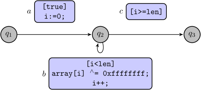
b CFG for function f

⬇

void g(int* array, uint len)

{

if(len%2==1) {

*array ^= 0xffffffff;

array++;

len--;

}

while(len) {

*((long*)array) ^=

0xffffffffffffffff;

array += 2;

len -= 2;

}

}

c Function g

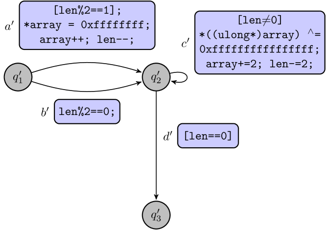
d CFG for function g

Figure 1: Functions and their CFGs

Checking equivalence of programs is an important problem due to its many diverse applications, including translation validation and compiler correctness [21, 13, 19], code refactoring [23], program synthesis [3], hypersafety verification [1, 8, 26], superoptimization [24, 5], and software engineering education [16], amongst many others. In general, depending on the application, the criteria for equivalence may be weaker or stronger. For instance, the condition may be that all the observables including the machine state (stack, heap, and registers) are equal, or that only a subset of them are. Informally and broadly speaking, techniques that handle this problem try to put the two programs together in a way that makes it easier to justify the semantic equivalence. Note that one may always combine the programs naively, like in a sequential composition where they are run one after the other, but then arguing becomes difficult because it necessitates that every component be analyzed fully. Consider an example (borrowed from [4]) shown in Fig. 1. There are two functions $f$ and $g$, both of which take two parameters as input: array, which points to an array of 32-bit integers, and len which stores the length of the array. The function $f$ flips the bits of the array elements by iterating over each array element, and function $g$ flips 64 bits from wherever the array is pointing to, and then moves the array pointer to the end of the flipped bits. In the beginning, however, $g$ checks whether len is odd and if so, flips only 32 bits for the first time, and then continues flipping 64 at a time as described before. To establish that the programs are semantically equivalent, one may simply put the two programs together, one after another as sequential components of a single program, and assert the equivalence condition at the end. But, to analyze this combined program, one must learn completely what is happening in $f$, and also in $g$, and thereby conclude that they are indeed doing the same thing.

The equivalence checking technique presented in [4], on which we build, takes two programs and set of test cases, and constructs a trace alignment for every test case. The trace alignment is essentially a pairing of states in the execution traces of the programs, corresponding to a test case. This construction is guided by an alignment predicate that helps in pairing the states semantically. The technique then builds the product program as a program alignment automaton (PAA), and then learns invariants for all its states to establish the equivalence. In fact, the test cases are split into two sets – to be used for training and testing – in the beginning, and along with a set of candidate alignment predicates, a trace alignment and a PAA are learned from the training data. In this setting, it becomes important to ensure that the PAA does not overfit the training data. Therefore, its viability is checked using the testing set. A PAA is acceptable only if it soundly overapproximates the two programs, and is rejected otherwise. In the latter case, the search for an acceptable PAA continues with a different alignment predicate. Their technique benefits from choosing a good alignment predicate that allows to capture all possible pairs of program executions, including those from the testing set, even though it was learned from the training data alone.

The advantage of a semantic alignment is that it can see through the syntactic differences. However, there are also drawbacks of a trace-based technique: a) obtaining traces that cover all program behaviors is difficult, and any under-approximation may lead to an incomplete product program, and b) an indirect construction of this kind is unaware of the missing behaviors, and has no control over the aforesaid incompleteness. Alternatively, there are techniques that do not need traces to arrive at a product program, but they make assumptions that are strongly limiting [7]. In this work, we propose an algorithm for direct construction of PAA’s, that has the goodness of being guided by an alignment predicate, while still not needing any test cases or unrealistic assumptions.

The core contribution of this paper is an algorithm for predicate guided semantic program alignment without using traces, which we present in Sect. 2. This is followed by a step-by-step illustration of it on the example of Fig. 1, in Sect. 3. We present another illustrative run on an example involving arrays, which emphasizes the usefulness of our direct construction over a trace-based technique, in Sect. 4. This is followed by a short note on disjunctive invariants (in Sect. 5), a discussion of the related work (in Sect. 6), and our concluding remarks (in Sect. 7).

2 Equivalence Checking Algorithm

Algorithm 1 Equivalence checking

1:$\mathcal{A}_{paa}\leftarrow\mathit{paaConstruct}$ ($f,g,\mathcal{P}_{align}$)

2:$\mathcal{A}^{inv}_{paa}\leftarrow\mathit{learnInvariants}$($\mathcal{A}_{paa}$)

3:if final-state invariant of $\mathcal{A}^{inv}_{paa}\Rightarrow$ equiv. prop then

4:     return equivalent

5:return unknown

Alg. 1 shows the procedure for checking equivalence of two programs, $f$ and $g$. Given the programs and an alignment predicate $\mathcal{P}_{align}$, it builds a program alignment automaton, learns invariants for every state in the PAA, and then checks if the invariants in the final state discharge the equivalence goal. The learned invariants need to be consistent with the PAA, in the sense that if one picks an edge in the PAA, then the invariants at the target state must follow from the ones at the source, and the label on the chosen edge.

The inputs to the procedure $\mathit{paaConstruct}$ in Alg. 2 are automata $\mathcal{A}_{P_{1}}$ and $\mathcal{A}_{P_{2}}$, which are CFGs of $f$ and $g$ resp., and an alignment predicate $\mathcal{P}_{\mathit{align}}$. We assume that each program/function has unique entry and exit state, $q_{init}$ and $q_{exit}$, akin to initial and final state in an automaton. The procedure collects the states of both the automata, and defines the states, $\mathcal{S}$, of the PAA to be their product, i.e. each state in $\mathcal{S}$ is a tuple of two states $(q_{i},q_{j})$, one from each automaton. The initial product state (which is simply the product of the initial states) is marked reachable using the set $\mathit{Reach}$, and the transitions ($\mathcal{T}$, an empty set in the beginning) are populated one at a time, in a while loop (lines $7$-$20$).

In each iteration of the loop, a source state $(q_{i_{1}},q_{{j_{1}}})$ is chosen as any unvisited state from the reachable set $Reach$ (as is marked visited immediately), along with a target state $(q_{i_{2}},q_{{j_{2}}})$ from $\mathcal{S}$ (lines $7$-$9$). Then, the procedure derives a regular expression denoting words in automaton $\mathcal{A}_{P_{1}}$, corresponding to paths beginning at $q_{i_{1}}$ and ending at $q_{i_{2}}$. And, similarly, another regular expressions for words in $\mathcal{A}_{P_{2}}$, for paths beginning at $q_{j_{1}}$ and ending at $q_{j_{2}}$. At this point, it discards this source-target pair if the regular expression corresponds to an empty set in any of the automata. It also makes a discard if the source and target states are the same, and the regular expression for any of them is the empty word $\epsilon$. Intuitively, a discard of the former kind means that the target is simply not reachable from the source in the product program, whereas one of the latter kind denotes one of the programs is stuck in a no-progress cycle. One may also discard aggressively, e.g. if the program states in the target are not immediate neighbours of those in the source, but this may come at the cost of completeness (feasible program behaviours missing from the PAA).

The regular expressions are split over the top-level or (+) to deal with the different paths one at a time. This results into the sets $R_{i}$ and $R_{j}$, obtained by splitting $rex_{i}$ and $rex_{j}$ resp., as shown in line $14$. For every combination of paths (or, in other words, for every pair of regular expression $r_{i}\in R_{i}$ and $r_{j}\in R_{j}$), the expressions are instantiated by replacing $*$’s with symbolic constants $k_{i}$’s. The decision whether there is a solution for the $k_{i}$’s in the instantiated expressions, such that an appropriate edge labeling can be obtained, is left to an SMT solver (see Sect. 2.3). An edge is added between a source and a target state only if the alignment predicate can be propagated along the edge. Line $17$ of the pseudocode encodes this check. If an edge is added, the target state is added to the $\mathit{Reach}$ set with an unvisited mark.

Algorithm 2 The program alignment automaton construction algorithm

1:procedure $\mathit{paaConstruct}$ ($\mathcal{A}_{P_{1}},\mathcal{A}_{P_{2}},\mathcal{P}_{\mathit{align}}$)

2:     $S_{1}\leftarrow$ states of $\mathcal{A}_{P_{1}}$

3:     $S_{2}\leftarrow$ states of $\mathcal{A}_{P_{2}}$

4:

5:     $\mathcal{S}\leftarrow$ {($q_{i},q_{j}$)} where $q_{i}\in S_{1},q_{j}\in S_{2}$ $\triangleright$ set of product states

6:     $\mathit{Reach}\leftarrow\{(q_{init_{1}},q_{init_{2}})\}$ $\triangleright$ $q_{init_{i}}$ is the start state of automaton $\mathcal{A}_{P_{i}}$

7:     $\mathcal{T}\leftarrow\emptyset$

8:

9:     while $\mathit{Reach}$ has a state $(q_{i_{1}},q_{{j_{1}}})$, not yet marked visited do

10:         mark $(q_{i_{1}},q_{{j_{1}}})$ as visited

11:         for $(q_{i_{2}},q_{{j_{2}}})\in\mathcal{S}$ do $\triangleright$ picking a target state to find transitions

12:              $rex_{i}\leftarrow$ $\mathcal{L}$($\mathcal{A}_{P_{1}}$, with $q_{i_{1}}$ as initial and $q_{i_{2}}$ as final states)

13:              $rex_{j}\leftarrow$ $\mathcal{L}$($\mathcal{A}_{P_{2}}$, with $q_{j_{1}}$ as initial and $q_{j_{2}}$ as final states)

14:$\triangleright$ discard the state-pair in case of no paths, or if there is a no-progress cycle

15:              $\mathbf{next}$ if ($rex_{i}$ = $\emptyset$) or ($rex_{j}$ = $\emptyset$)

16:              $\mathbf{next}$ if ($q_{i_{1}}$ = $q_{i_{2}}$ and $q_{j_{1}}$ = $q_{j_{2}}$) and ($rex_{i}=\{\epsilon\}$ or $rex_{j}=\{\epsilon\}$)

17:

18:              $R_{i}\leftarrow\mathit{split}$($rex_{i}$); $R_{j}\leftarrow\mathit{split}$($rex_{j}$)

19:              for $(r_{i},r_{j})\in R_{i}\times R_{j}$ do

20:                  ${r^{c}}_{i},{r^{c}}_{j}$ $\leftarrow\mathit{instantiate}$($r_{i},r_{j}$) $\triangleright$ replace $\ast$ with constants $k_{i}$’s

21:                  find min $k_{i}$’s: $\mathcal{P}_{\mathit{align}}\wedge{r^{c}}_{i}\wedge{r^{c}}_{j}\Rightarrow\overline{\mathcal{P}}_{\mathit{align}}$ $\triangleright$ $\overline{~{}\cdot~{}}$ denotes next-state

22:                  if a solution is found then

23:                       $\mathcal{T}\leftarrow\mathcal{T}~{}~{}\cup~{}~{}(q_{i_{1}},q_{j_{1}})\xrightarrow{{r^{c}}_{i};{r^{c}}_{j}}(q_{i_{2}},q_{j_{2}})$

24:                       $Reach\leftarrow Reach\cup\{(q_{i_{2}},q_{j_{2}})\}$                                               

25:

26:     $\mathcal{S}\leftarrow Reach$ $\triangleright$ unreached states are removed from $\mathcal{S}$ in the end

27:     $\mathit{simplify}(\mathcal{T},\mathcal{S})$

The while loop exits when all the reachable states have been marked visited. At this point the unreached states are removed from $S$, and the resulting set along with the set of transitions $\mathcal{T}$, describes the program alignment automaton obtained thus. The resulting PAA is also simplified, in a manner similar to [4], as explained in Sect. 2.2.

The usefulness of an alignment predicate reflects in how well it helps align the programs and discharge the equivalence property. For example, if an alignment predicate only helps to align the initial and the final states, and no other state in between, it does not make the proof any more easier than completely analysing the programs independently. Finding good alignment predicates is thus important, but also quite challenging at the same time [4]. Though we do not address this problem here, we believe that data- and syntax-guided techniques can be quite helpful in making this practicable. For example, the technique in [4] learns a set of candidate alignment predicates from the training data. Similarly, one may construct a grammar and sample these candidates automatically from the program source following the ideas of [9, 22, 10].

2.1 Propagating preconditions along transitions

In addition to the alignment predicate, there are also predicates that capture the preconditions under which we are checking equivalence. This could, for instance, be a predicate equating the input variables of the two programs. Let $\mathcal{P}_{\mathit{input}}$ denote a set of such predicates. When a transition is added to the PAA, the predicates in this set are also propagated to the target state if they hold there. These predicates help in the propagating the alignment predicate by strengthening the premise of the check in line $17$. If the alignment predicate can be propagated along an edge without the help of these input predicates, then the edge is added as it is. Otherwise, if it is propagated with the assistance of the input predicates, then the edge is marked (as “dependent on an input predicate”) before it is added to a set of marked transitions, $\mathcal{T}_{m}$ (instead of $\mathcal{T}$). Once the PAA construction is over, if an input predicate has not been propagated to any state, we remove all marked edges from the state that are dependent on that predicate.

The reason we separate the marked transitions from the unmarked ones is to avoid backtracking. A predicate $p\in\mathcal{P}_{\mathit{input}}$ holds at a non-initial state $s$ only if it is preserved along all paths that reach $s$. At an intermediate stage in the construction, even if $p$ holds at $s$, it may later be discovered to not hold there. However, if $p$ was used at that stage to propagate the alignment predicate, we would need to remove that edge and backtrack. Marking such transitions and keeping them separately allows us to get rid of all of them, at once, in the end.

2.2 Reduction of Program Alignment Automaton

The procedure $\mathit{simplify~{}}(\mathcal{T},\mathcal{S})$ reduces the program alignment automaton for $\mathcal{P}_{align}$ by repeatedly applying the following two reductions, as long as they have some effect.

1. $\mathit{RemoveStates~{}}$ removes every state $s$, other than the initial and the final state, that does not have a self-loop. Essentially, it replaces each pair of transitions $s_{k}\xrightarrow{P;Q}s$ and $s\xrightarrow{P^{\prime};Q^{\prime}}s_{l}$, where $s$ does not have a self-loop, with a transition $s_{k}\xrightarrow{}s_{l}$ labeled with $PP^{\prime};QQ^{\prime}$.

2. $\mathit{RemoveTransitions~{}}$ removes transitions of the form $s\xrightarrow{P^{\prime};Q^{\prime}}s_{k}$, if there is a transition $s\xrightarrow{P;Q}s_{l}$ where $P$ is a prefix of $P^{\prime}$ and $Q$ is a prefix of $Q^{\prime}$.

2.3 Concretization of regular expressions

While adding transitions in the PAA, we employ a solver to compute valid solutions of $k_{i}$’s in the instantiated regular expressions. In this subsection, we describe why it is sufficient to find these instantiations such that they account for all program behaviours. In our PAA construction, there can be three types of the transition labels $P;Q$.

1. Both $P$ and $Q$ contain loop blocks, i.e. the label is of form $r_{i}r_{i}^{k_{1}};r_{j}r_{j}^{k_{2}}$ where $r_{i}$ and $r_{j}$ are the blocks denoting loops in respective functions. In this case, we find the minimum values of $k_{1}$ and $k_{2}$ such that $k_{1}+1$ iterations of $r_{i}$ are aligned with $k_{2}+1$ iterations of $r_{j}$. By not considering their minimum values, we will be unable to account for the behaviours with smaller number of loop iterations. However, minimum values automatically accommodate behaviors with higher number of loop iterations.

2. Only one of $P$ and $Q$ has a loop block, i.e. the label is of one of the forms $r_{i-1}r_{i}^{k};r_{j}$, $r_{i}^{k}r_{i+1};r_{j}$, $r_{i};r_{j}^{k}r_{j+1}$ or $r_{i};r_{j-1}r_{j}^{k}$, where the expression with superscript $k$ denotes the loop block. In this case, we check if there exists a value of $k$ such that the transition preserves the validity of alignment predicate. Intuitively, this value of $k$ determines how many iterations of loop in one function are aligned with a non-loop block in other function.

3. Neither $P$ nor $Q$ has a loop block, i.e. the label is $r_{i};r_{j}$. Here, merely checking that taking this transition does not violate the alignment predicate is sufficient.

3 Illustrative run on an example

We use the example in Fig. 1 to illustrate Alg. 2. The inputs to $\mathit{paaConstruct}$ are the automata shown in figures 1b and 1d, and an alignment predicate $\mathcal{P}_{align}$: $array+4i=array^{\prime}$. The sets $S_{1}$ and $S_{2}$ are $\{q_{1},~{}q_{2},~{}q_{3}\}$ and $\{q^{\prime}_{1},~{}q^{\prime}_{2},~{}q^{\prime}_{3}\}$ (resp.), and thus the PAA has nine possible states $\{q_{1}q^{\prime}_{1},~{}q_{1}q^{\prime}_{2},~{}\ldots,~{}q_{3}q^{\prime}_{2},~{}q_{3}q^{\prime}_{3}\}$. We often denote the product state $(q_{i},q_{j})$ as $q_{i}q_{j}$. The states $q_{1}q^{\prime}_{1}$ and $q_{3}q^{\prime}_{3}$ are marked as initial and final, resp. We assume that the alignment predicate holds in the initial state, without evaluating whether it actually holds or not. As described in Sect 2.1, we also have a set of input predicates (omitted from Alg. 2 for ease of exposition) that hold in the beginning. In this example, it is the set $\{array=array^{\prime},len=len^{\prime},\omega=\omega^{\prime}\}$, where $\omega$ denotes the heap state. The predicate $\omega=\omega^{\prime}$ is the precondition that the programs execute from the same heap state. Input predicates holds at the initial state, and at any subsequent state unless a transition flips their truth value.

Table 1: Computing PAA transitions

Row	Transition	Regex	Instantiation	Label	Set
1	$q_{1}q^{\prime}_{1}\xrightarrow{}q_{2}q^{\prime}_{1}$	$ab^{*};\epsilon$	$ab^{k_{1}};\epsilon$ ${\{{\scriptstyle k_{1}=0}\}}$	$a;\epsilon$	$\mathcal{T}_{m}$
2	$q_{1}q^{\prime}_{1}\xrightarrow{}q_{1}q^{\prime}_{2}$	$\epsilon;b^{\prime}c^{\prime*}+a^{\prime}c^{\prime*}$	$\epsilon;b^{\prime}c^{\prime k_{1}}$ $\{{\scriptstyle k_{1}=0}\}$	$\epsilon;b^{\prime}$	$\mathcal{T}$
			$\epsilon;a^{\prime}c^{\prime k_{2}}$ $\{{\scriptstyle k_{2}=-}\}$	$-$	$-$
3	$q_{1}q^{\prime}_{2}\xrightarrow{}q_{2}q^{\prime}_{1}$	$ab^{*};\emptyset$	no path from $q^{\prime}_{2}$ to $q^{\prime}_{1}$	$-$	$-$
4	$q_{1}q^{\prime}_{1}\xrightarrow{}q_{2}q^{\prime}_{2}$	$ab^{*};b^{\prime}c^{\prime*}+a^{\prime}c^{\prime*}$	$ab^{k_{1}};b^{\prime}c^{\prime k_{2}}$ $\{{\scriptstyle k_{1}=0,k_{2}=0}\}$	$a;b^{\prime}$	$\mathcal{T}_{m}$
			$ab^{k_{3}};a^{\prime}c^{\prime k_{4}}$ $\{{\scriptstyle k_{3}=1,k_{4}=0}\}$	$ab;a^{\prime}$	$\mathcal{T}_{m}$
5	$q_{2}q^{\prime}_{1}\xrightarrow{}q_{2}q^{\prime}_{1}$	$b^{*};\epsilon$	no-progress cycle ${\{{\scriptstyle-}\}}$	$-$	$-$
6	$q_{2}q^{\prime}_{1}\xrightarrow{}q_{2}q^{\prime}_{2}$	$b^{*};a^{\prime}c^{\prime*}+b^{\prime}c^{\prime*}$	$b^{k_{1}};a^{\prime}c^{\prime k_{2}}$ $\{{\scriptstyle k_{1}=1,k_{2}=0}\}$	$b;a^{\prime}$	$\mathcal{T}$
			$b^{k_{3}};b^{\prime}c^{\prime k_{4}}$ $\{{\scriptstyle k_{3}=0,k_{4}=0}\}$	$\epsilon;b^{\prime}$	$\mathcal{T}$
7	$q_{2}q^{\prime}_{1}\xrightarrow{}q_{3}q^{\prime}_{2}$	$b^{*}c;a^{\prime}c^{\prime*}+b^{\prime}c^{\prime*}$	$b^{k_{1}}c;a^{\prime}c^{\prime k_{2}}$ $\{{\scriptstyle k_{1}=1,k_{2}=0}\}$	$bc;a^{\prime}$	$\mathcal{T}$
			$b^{k_{3}}c;b^{\prime}c^{\prime k_{4}}$ $\{{\scriptstyle k_{3}=0,k_{4}=0}\}$	$c;b^{\prime}$	$\mathcal{T}$
8	$q_{2}q^{\prime}_{1}\xrightarrow{}q_{3}q^{\prime}_{1}$	$b^{*}c;\epsilon$	$b^{k_{1}}c;\epsilon$ ${\{{\scriptstyle k_{1}=0}\}}$	$c;\epsilon$	$\mathcal{T}$
9	$q_{1}q^{\prime}_{2}\xrightarrow{}q_{1}q^{\prime}_{3}$	$\epsilon;c^{\prime*}d^{\prime}$	$\epsilon;c^{\prime k_{1}}d^{\prime}$ ${\{{\scriptstyle k_{1}=0}\}}$	$\epsilon;d^{\prime}$	$\mathcal{T}$
10	$q_{1}q^{\prime}_{2}\xrightarrow{}q_{2}q^{\prime}_{2}$	$ab^{*};c^{\prime*}$	$ab^{k_{1}};c^{\prime k_{2}}$ ${\{{\scriptstyle k_{1}=0,k_{2}=0}\}}$	$a;\epsilon$	$\mathcal{T}_{m}$
11	$q_{1}q^{\prime}_{2}\xrightarrow{}q_{2}q^{\prime}_{3}$	$ab^{*};c^{\prime*}d^{\prime}$	$ab^{k_{1}};c^{\prime k_{2}}d^{\prime}$ ${\{{\scriptstyle k_{1}=0,k_{2}=0}\}}$	$a;d^{\prime}$	$\mathcal{T}_{m}$
12	$q_{3}q^{\prime}_{1}\xrightarrow{}q_{3}q^{\prime}_{2}$	$\epsilon;a^{\prime}c^{\prime*}+b^{\prime}c^{\prime*}$	$\epsilon;a^{\prime}c^{\prime k_{1}}$ $\{{\scriptstyle k_{1}=-}\}$	$-$	$-$
			$\epsilon;b^{\prime}c^{\prime k_{2}}$ $\{{\scriptstyle k_{2}=0}\}$	$\epsilon;b^{\prime}$	$\mathcal{T}$
13	$q_{1}q^{\prime}_{3}\xrightarrow{}q_{2}q^{\prime}_{3}$	$ab^{*};\epsilon$	$ab^{k_{1}};\epsilon$ ${\{{\scriptstyle k_{1}=0}\}}$	$a;\epsilon$	$\mathcal{T}_{m}$
14	$q_{2}q^{\prime}_{2}\xrightarrow{}q_{2}q^{\prime}_{2}$	$b^{*};c^{\prime*}$	$bb^{k_{1}};c^{\prime}c^{\prime k_{2}}$ ${\{{\scriptstyle k_{1}=1,k_{2}=0}\}}$	$bb;c^{\prime}$	$\mathcal{T}$
15	$q_{2}q^{\prime}_{2}\xrightarrow{}q_{2}q^{\prime}_{3}$	$b^{*};c^{\prime*}d^{\prime}$	$b^{k_{1}};c^{\prime k_{2}}d^{\prime}$ ${\{{\scriptstyle k_{1}=0,k_{2}=0}\}}$	$\epsilon;d^{\prime}$	$\mathcal{T}$
16	$q_{2}q^{\prime}_{2}\xrightarrow{}q_{3}q^{\prime}_{2}$	$b^{*}c;c^{\prime*}$	$b^{k_{1}}c;c^{\prime k_{2}}$ ${\{{\scriptstyle k_{1}=0,k_{2}=0}\}}$	$c;\epsilon$	$\mathcal{T}$
17	$q_{2}q^{\prime}_{2}\xrightarrow{}q_{3}q^{\prime}_{3}$	$b^{*}c;c^{\prime*}d^{\prime}$	$b^{k_{1}}c;c^{\prime k_{2}}d^{\prime}$ ${\{{\scriptstyle k_{1}=0,k_{2}=0}\}}$	$c;d^{\prime}$	$\mathcal{T}$
18	$q_{2}q^{\prime}_{3}\xrightarrow{}q_{3}q^{\prime}_{3}$	$b^{*}c;\epsilon$	$b^{k_{1}}c;\epsilon$ ${\{{\scriptstyle k_{1}=0}\}}$	$c;\epsilon$	$\mathcal{T}$
19	$q_{3}q^{\prime}_{2}\xrightarrow{}q_{3}q^{\prime}_{3}$	$\epsilon;c^{\prime*}d^{\prime}$	$\epsilon;c^{\prime k_{1}}d^{\prime}$ ${\{{\scriptstyle k_{1}=0}\}}$	$\epsilon;d^{\prime}$	$\mathcal{T}$
20	$q_{1}q^{\prime}_{3}\xrightarrow{}q_{1}q^{\prime}_{3}$	$\epsilon;\epsilon$	no-progress cycle ${\{{\scriptstyle-}\}}$	$-$	$-$

We mark the initial state $q_{1}q^{\prime}_{1}$ as reachable by initializing the set $Reach$ with it (line $5$). We also initialize the transition set $\mathcal{T}$ to be an empty set. The process of adding a transition begins by picking two states: a source state from the $Reach$, and a target from $\mathcal{S}$. Table 1 shows all the transitions that were added by the algorithm. In what follows, we describe a few interesting cases in details.

Single transition Consider the pair of states $q_{1}q^{\prime}_{1}\in Reach$ and $q_{2}q^{\prime}_{1}\in\mathcal{S}$ at the entry 1 in Table 1. We mark $q_{1}q^{\prime}_{1}$ as visited before proceeding (line $8$). The regular expression $ab^{*}$ denotes all the words beginning at $q_{1}$ and ending at $q_{2}$ in Fig. 1b (line $10$). Similarly, $\epsilon$ denotes the words starting at $q^{\prime}_{1}$ and ending at $q^{\prime}_{1}$ in Fig. 1d (line $11$). Since these expressions do not have a top-level or (denoted by ‘$+$’), we just get two singleton sets – $\{ab^{*}\}$ and $\{\epsilon\}$ – in line $14$. Recall that, by assumption, both $\mathcal{P}_{align}$ and $\mathcal{P}_{input}$ hold at $q_{1}q^{\prime}_{1}$. We employ an SMT solver to find an instantiation, if one exists, of $ab^{k_{1}};\epsilon$, such that $\mathcal{P}_{align}$ retains its truth value at $q_{2}q^{\prime}_{1}$ after taking the transition (lines $16-19$). In particular, we solve the query $array+4i=array^{\prime}\land ab^{k_{1}}\land\epsilon\implies\overline{array}+4\overline{i}=\overline{array}^{\prime}$ for the minimum value of $k_{1}$. As the solver does not find any satisfying assignment, we try to solve the query by adding $\mathcal{P}_{input}$ to the premise. The solver now returns $0$ as the solution which results into a transition $q_{1}q^{\prime}_{1}\xrightarrow{a;\epsilon}q_{2}q^{\prime}_{1}$. We add this transition to $\mathcal{T}_{m}$ (see Sect. 2.1) and add $q_{2}q^{\prime}_{1}$ to $Reach$ (lines $20-22$). Further, since the basic block $a$ in Fig. 1b does not affect the truth value of $\mathcal{P}_{input}$, we propagate $\mathcal{P}_{input}$ to $q_{2}q^{\prime}_{1}$ through this transition by making a similar query to the solver.

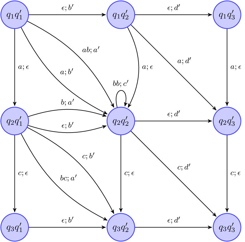
Figure 2: PAA for Fig. 1

Let us pick another pair of states: $q_{1}q^{\prime}_{1}$ and $q_{1}q^{\prime}_{2}$, the second entry in Table 1. The regular expressions denoting the words between component states are $\epsilon$ and $b^{\prime}c^{\prime*}+a^{\prime}c^{\prime*}$, and splitting gives two sets - $\{\epsilon\},\{b^{\prime}c^{\prime*};a^{\prime}c^{\prime*}\}$. We solve two queries in order to obtain their instantiations: (i) $array+4i=array^{\prime}\land\epsilon\land b^{\prime}c^{\prime k_{1}}\implies\overline{array}+4\overline{i}=\overline{array}^{\prime}$, and (ii) $\mathcal{P}_{\mathit{input}}\land array+4i=array^{\prime}\land\epsilon\land a^{\prime}c^{\prime k_{2}}\implies\overline{array}+4\overline{i}=\overline{array}^{\prime}$. For the first query, the solver provides $k_{1}=0$. We add a transition $q_{1}q^{\prime}_{1}\xrightarrow{\epsilon;b^{\prime}}q_{1}q^{\prime}_{2}$ to $\mathcal{T}$ and add $q_{1}q^{\prime}_{2}$ to $Reach$. Notice that we added $\mathcal{P}_{input}$ to the premise in second query after we observed that the solver could not find an instantiation without $\mathcal{P}_{input}$. The second query could not be solved, even with $\mathcal{P}_{input}$. We propagate $\mathcal{P}_{input}$ to $q_{1}q^{\prime}_{2}$, as it is not affected by the edge labeled $\epsilon;b^{\prime}$.

Discarding a pair of states Consider a pair $q_{1}q^{\prime}_{2}$ and $q_{2}q^{\prime}_{1}$ at entry $3$ in Table 1. Note that there is a path from $q_{1}$ to $q_{2}$ in the automaton in Fig. 1b but there is no path from $q^{\prime}_{2}$ to $q^{\prime}_{1}$ in  1d. So, we discard this pair since no transition can be added from $q_{1}q^{\prime}_{2}$ to $q_{2}q^{\prime}_{1}$ (line $12$ in Alg. 2). Consider another pair, $q_{2}q^{\prime}_{1}$ and $q_{2}q^{\prime}_{1}$, at entry $5$. The associated regex $b^{*};\epsilon$ represents all the words starting at $q_{2}q^{\prime}_{1}$ and ending at $q_{2}q^{\prime}_{1}$. As this expression would result into a no-progress cycle (the states does not change in any of the components, and at least one of the expressions is $\epsilon$) at $q_{2}q^{\prime}_{1}$, we discard this pair (line $13$ in Alg. 2).

In this example, we only look for the pairs where component states are immediate neighbors in respective automaton. For instance, we do not look for a transition between $q_{1}q^{\prime}_{1}$ and $q_{1}q^{\prime}_{3}$ because $q^{\prime}_{1}$ and $q^{\prime}_{3}$ are not immediate neighbors in Fig. 1d. Such optimizations, in general, may lead to loss of behaviours.

Multiple transitions For the pair $q_{2}q^{\prime}_{1}$ and $q_{2}q^{\prime}_{2}$ at entry $6$, the regular expressions are $b^{*}$ and $a^{\prime}c^{\prime*}+b^{\prime}c^{\prime*}$. Splitting gives us the sets: $\{b^{*};a^{\prime}c^{\prime*}\}$ and $\{b^{*};b^{\prime}c^{\prime*}\}$. The solver returns $k_{1}=1,k_{2}=0$ as the instantiation of $b^{k_{1}};a^{\prime}c^{\prime k_{2}}$, which gives the edge label $b;a^{\prime}$. For the other component, $b^{k_{3}};b^{\prime}c^{\prime k_{4}}$, the transition label becomes $\epsilon;b^{\prime}$ as the solver return $k_{3}=0,k_{4}=0$. These were obtained with $\mathcal{P}_{input}$ in the premise, and thus, are added to $\mathcal{T}$. The state $q_{2}q^{\prime}_{2}$ is added to $Reach$. Observe that the truth values of $array=array^{\prime}$ and $len=len^{\prime}$ are affected by the blocks $b$ and $a^{\prime}$, therefore these are dropped at the target state. However, since $\omega=\omega^{\prime}$ is still unaffected, we propagate it to $q_{2}q^{\prime}_{2}$.

Self-loop The transition $b^{*};c^{\prime*}$ at entry 14 corresponds to a self-loop at the state $q_{2}q^{\prime}_{2}$. We get $k_{1}=2,k_{2}=1$ as the instantiation of $bb^{k_{1}};c^{\prime}c^{\prime k_{2}}$ using the solver, and add a self-loop with label $bb;c^{\prime}$ at $q_{2}q^{\prime}_{2}$. Informally, it shows that a transition with two iterations of $b$ and one iteration of $c^{\prime}$ preserves the satisfiability of $\mathcal{P}_{align}$ at $q_{2}q_{2}^{\prime}$. Note that we do not enquire for minimum values of $k_{i}$’s in the case of $b^{k_{1}};c^{\prime k_{2}}$, because the minimum ($k_{1}=0,k_{2}=0$) corresponds to a no-progress cycle. The query is suitably modified for self-loops to ensure progress.

a After removing states $q_{1}q^{\prime}_{3}$ and $q_{3}q^{\prime}_{1}$

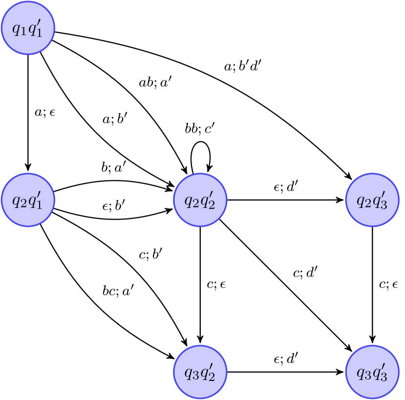
b After removing state $q_{1}q^{\prime}_{2}$

Figure 3: Reduction of PAA in Figure 2

Once the while loop ends, the unreachable states are removed from $\mathcal{S}$, and the valid transition of $\mathcal{T}_{m}$ are added to $\mathcal{T}$. A marked transition is valid if the input predicates used in the premise continue to be available at the source state in the end. The PAA thus constructed, shown in Fig. 1, is then simplified. For instance, we can remove state $q_{1}q^{\prime}_{3}$ by replacing transitions $q_{1}q^{\prime}_{2}\xrightarrow{\epsilon;d^{\prime}}q_{1}q^{\prime}_{3}$ and $q_{1}q^{\prime}_{3}\xrightarrow{a;\epsilon}q_{2}q^{\prime}_{3}$ with a transition $q_{1}q^{\prime}_{2}\xrightarrow{a;d^{\prime}}q_{2}q^{\prime}_{3}$ which is already present. The reduced PAA is shown in Fig. 3a. In a similar manner, state $q_{1}q^{\prime}_{2}$ is removed by replacing - (i) the transitions $q_{1}q^{\prime}_{1}\xrightarrow{\epsilon;b^{\prime}}q_{1}q^{\prime}_{2}$ and $q_{1}q^{\prime}_{2}\xrightarrow{a;d^{\prime}}q_{2}q^{\prime}_{3}$ with a transition $q_{1}q^{\prime}_{1}\xrightarrow{a;b^{\prime}d^{\prime}}q_{2}q^{\prime}_{3}$, (ii) the transitions $q_{1}q^{\prime}_{1}\xrightarrow{\epsilon;b^{\prime}}q_{1}q^{\prime}_{2}$ and $q_{1}q^{\prime}_{2}\xrightarrow{a;\epsilon}q_{2}q^{\prime}_{2}$ with a transition $q_{1}q^{\prime}_{1}\xrightarrow{a;b^{\prime}}q_{2}q^{\prime}_{2}$. Next, we remove the transition $q_{1}q^{\prime}_{1}\xrightarrow{a;b^{\prime}d^{\prime}}q_{2}q^{\prime}_{3}$ because there exists a transition $q_{1}q^{\prime}_{1}\xrightarrow{a;b^{\prime}}q_{2}q^{\prime}_{2}$ where $a$ is a prefix of $a$ and $b^{\prime}$ is a prefix of $b^{\prime}d^{\prime}$. We keep applying these reductions until the PAA can not be simplified further. The final PAA is shown in Fig. 4a. This is exactly same as the PAA obtained by the technique in [4]. However, since their technique depends on test cases, if the training set had only even len cases (for example), they would have ended up with a different PAA, shown in Fig. 4b. Observe that this PAA does not have a transition corresponding to edge $a^{\prime}$[len%2 = 1] in Fig. 1d, and therefore does not overapproximate all possible behaviors.

3.1 Learning Invariants and Discharging Proof Obligations

Though we do not have any contributions here, we illustrate how this is done (in [4]) to make the paper self-contained.

Once a PAA is constructed, invariants are learned for each state. These invariants must be consistent with PAA i.e, for each transition $s\xrightarrow{P;Q}t$, if $\phi_{s}$ and $\phi_{t}$ are the invariants at state $s$ and $t$ respectively, then, $\{\phi_{s}\}~{}P;Q~{}\{\phi_{t}\}$ must be valid. The aim is to learn sufficiently strong invariants at the final state, so that the equivalence property can be discharged. There are several techniques that have been proposed to learn such invariants [4, 7], including those that aim to learn them from the program’s syntactic source, e.g. [9].

It must be first argued that the constructed PAA overapproximates all program behaviors. Consider the initial state $q_{1}q^{\prime}_{1}$: the state $q_{1}$ in $f$ has one outgoing transition with its guard predicate as $true$ (say, $\alpha$), whereas, $q^{\prime}_{1}$ has two outgoing transitions with guard predicates $len\%2=0$ ($\beta$) and $len\%2=1$ ($\gamma$). Hence there are two possible transitions $\alpha\beta$ and $\alpha\gamma$ at $q_{1}q^{\prime}_{1}$, which are included in our PAA. For the state $q_{2}q^{\prime}_{2}$, it can be shown that the behaviours that are not present in the PAA are in fact infeasible. There are two possible behaviors at $q_{2}$: $i\geq len$ ($\alpha$) and $i<len$ ($\beta$); similarly, there are two behaviors at $q^{\prime}_{2}$: $len^{\prime}=0$ ($\gamma$) and $len^{\prime}\neq 0$ ($\delta$). Thus there are four possible behaviors at $q_{2}q^{\prime}_{2}$: $\alpha\gamma$, $\alpha\delta$, $\beta\gamma$, and $\beta\delta$. Since the behaviors $\alpha\gamma$ and $\beta\delta$ are already included in the PAA, showing that $\alpha\delta$ and $\beta\gamma$ are infeasible is sufficient. Observe that at state $q_{2}q^{\prime}_{2}$, the predicate $len-i=len^{\prime}\land i\leq len$ is an invariant. Since $i\geq len\land len^{\prime}\neq 0\land len-i=len^{\prime}\land i\leq len$ is unsatisfiable, the behavior $\alpha\delta$ is infeasible. Similarly, $i<len\land len^{\prime}=0\land len-i=len^{\prime}\land i\leq len$ is unsatisfiable which implies $\beta\gamma$ is infeasible.

We now justify why $len-i=len^{\prime}\land i\leq len$ is an invariant at $q_{2}q^{\prime}_{2}$. Initially at $q_{1}q^{\prime}_{1}$, $len$ and $len^{\prime}$ are same and non-negative. There are two ways to reach $q_{2}q^{\prime}_{2}$ from $q_{1}q^{\prime}_{1}$ depending on the parity of $len$. If $len$ is even, both $len$ and $len^{\prime}$ remain intact and $i$ is initialized to $0$. If $len$ is odd, there is no change in $len$ and $i$ becomes $1$, however, $len^{\prime}$ is decreased by $1$. Therefore, $len-i=len^{\prime}\land i\leq len$ is initially true at $q_{2}q^{\prime}_{2}$. Now, we prove the consecution. Assume at any step, the predicate $len-i=len^{\prime}\land i\leq len$ holds. Since the self-loop at $q_{2}q^{\prime}_{2}$ executes $b$ twice and $c^{\prime}$ once, it preserves the satisfiability of $len-i=len^{\prime}\land i\leq len$: $i$ increases by $2$ and $len^{\prime}$ decreases by $2$. Therefore, it’s an invariant at $q_{2}q^{\prime}_{2}$. Note that $\omega=\omega^{\prime}$ holds at $q_{2}q^{\prime}_{2}$, which is further propagated to $q_{3}q^{\prime}_{3}$ via transition $c;d^{\prime}$. It concludes that the two programs are equivalent since the content of the arrays or final heaps are same.

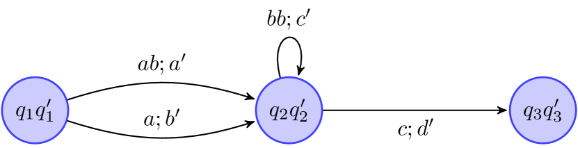
a proposed construction

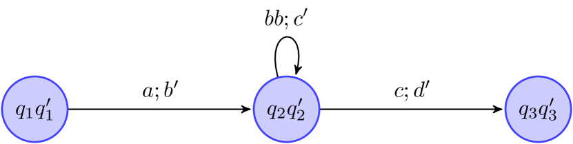
b using [4], and only even len traces

Figure 4: Final program alignment automaton

3.2 Soundness of our approach

Our approach is sound by construction. An edge is added in the PAA if and only if its source and target states are indeed connected through the transition-label. The choice of alignment predicates, and the inherent incompleteness of the technique, may sometimes result in a PAA that’s insufficient to establish equivalent (for example, if it does not capture all possible program behaviors). However, if a PAA and the learned invariants logically establish the equivalence, the programs are indeed equivalent.

4 Illustration on another example: arrayInsert

We underline the usefulness of our direct construction, as compared to the trace-based technique, using another example borrowed from [26]. Consider two copies, $f$ and $g$, of a program arrayInsert, as shown in Fig. 5; their CFGs are shown in Fig. 6. The program takes 3 input parameters: array $A$, its length len and an integer $h$. The precondition under which the equivalence is to be established is $A=A^{\prime}$ and $len=len^{\prime}$. The variables $h$ and $h^{\prime}$ are unconstrained by the precondition.

⬇

arrayInsert(A, len, h)

{

i = 0;

while (i<len && A[i]<h)

i++;

len = shift_array(A,i,1);

A[i] = h;

while (i<len) { i++; }

return i;

}

a Copy $f$

⬇

arrayInsert(A, len, h)

{

i = 0;

while (i<len && A[i]<h)

i++;

len = shift_array(A,i,1);

A[i] = h;

while (i<len) { i++; }

return i;

}

b Copy $g$

Figure 5: Copies of arrayInsert program

The task here is to insert $h$ at its appropriate position in the sorted array $A$, with the underlying assumption that $h$ is sensitive information and the place where it is inserted must not be leaked. To achieve this, the programs have a proxy loop towards the end, to move the counter $i$ to the end, independent of the position where $h$ was inserted. The postcondition for equivalence is that the output $i$ is the same for both the programs.

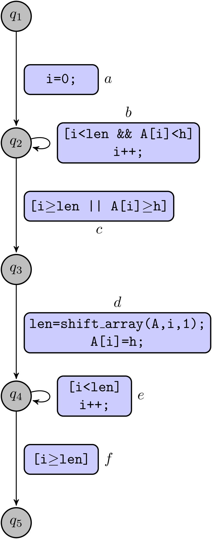
a Program $f$ automaton

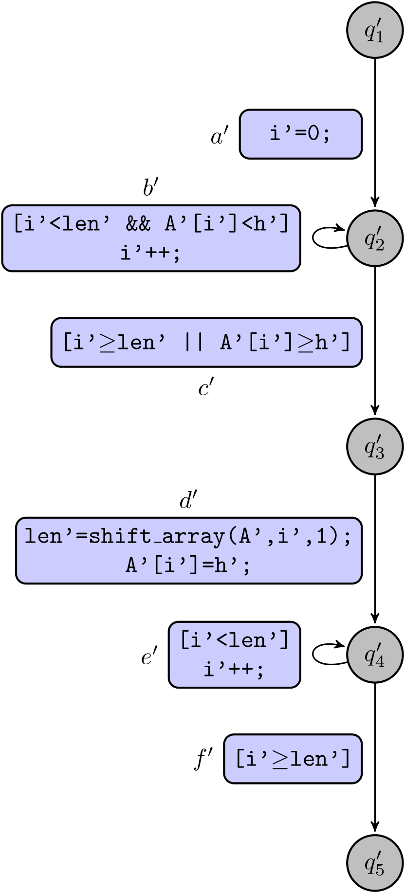
b Program $g$ automaton

Figure 6: Control flow graphs for Fig. 5 programs

Naturally, in this case, the predicate $i=i^{\prime}$ appears to be a good candidate for the alignment predicate $\mathcal{P}_{align}$ to construct a PAA. There are 3 scenarios based on the values of parameter h across both copies: (i) $h=h^{\prime}$ or both inserted at the same position in respective arrays, (ii) $h<h^{\prime}$ where $h$ and $h^{\prime}$ are inserted at different positions, and (iii) $h>h^{\prime}$ and both are inserted at different positions. The trace-based technique in  [4] would require a different pair of executions for computing the trace alignment in each scenario. Fig. 7 illustrates the program alignment automata constructed for each of these cases. Absence of any of the pairs would lead to missing behaviors in the final PAA. In contrast, our approach gives the PAA shown in Fig. 8. We argue that this PAA observes each scenario and overapproximates all behaviors.

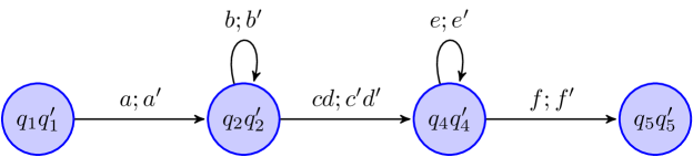
a Trace based PAA for $h=h^{\prime}$ or $h$ an $h^{\prime}$ are inserted at same positions

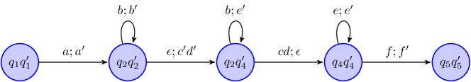
b Trace based PAA for $h>h^{\prime}$ where $h$ and $h^{\prime}$ are inserted at different positions

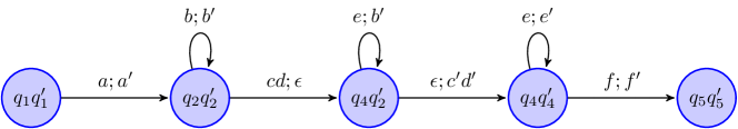
c Trace based PAA for $h<h^{\prime}$ where $h$ and $h^{\prime}$ are inserted at different positions

Figure 7: Trace PAAs for programs in Fig. 6

Consider the initial state $q_{1}q^{\prime}_{1}$: each of $q_{1}$ and $q^{\prime}_{1}$ has one outgoing transition with its guard predicate as $true$ (say, $\alpha$ and $\alpha^{\prime}$ resp.). Hence there is only one transition $\alpha\alpha^{\prime}$ at $q_{1}q^{\prime}_{1}$, which is included in the PAA. Now, let us consider the state $q_{2}q^{\prime}_{2}$. We show that the behaviours that are not present at $q_{2}q^{\prime}_{2}$ are actually infeasible. The same argument can be extended to rest of the states in similar manner. There are two behaviors possible at $q_{2}$: ($i<len\land A[i]<h$) (say, $\alpha$), ($i\geq len\lor A[i]\geq h$) ($\lnot\alpha$). Similarly, $q^{\prime}_{2}$ has two possible behaviors: ($i^{\prime}<len^{\prime}\land A^{\prime}[i^{\prime}]<h^{\prime}$) (say, $\gamma$), ($i^{\prime}\geq len^{\prime}\lor A^{\prime}[i^{\prime}]\geq h^{\prime}$) ($\lnot\gamma$). This leads to a total of four possible behaviors at $q_{2}q^{\prime}_{2}$: $\alpha\gamma$, $\lnot\alpha\gamma$, $\alpha\lnot\gamma$, and $\lnot\alpha\lnot\gamma$, as shown below. The alignment predicate $\mathcal{P}_{align}$ is $i=i^{\prime}$, and $len=len^{\prime}$ is a loop invariant at $q_{2}q^{\prime}_{2}$.

1. $\alpha\gamma$: ($i<len\land A[i]<h$) $\land$ ($i^{\prime}<len^{\prime}\land A^{\prime}[i^{\prime}]<h^{\prime}$)

2. $\alpha\lnot\gamma$: ($i<len\land A[i]<h$) $\land$ ($i^{\prime}\geq len^{\prime}\lor A^{\prime}[i^{\prime}]\geq h^{\prime}$)

   1. ($i<len\land A[i]<h$) $\land$ $i^{\prime}\geq len^{\prime}$

   2. ($i<len\land A[i]<h$) $\land$ $A^{\prime}[i^{\prime}]\geq h^{\prime}$

3. $\lnot\alpha\gamma$: ($i\geq len\lor A[i]\geq h$) $\land$ ($i^{\prime}<len^{\prime}\land A^{\prime}[i^{\prime}]<h^{\prime}$)

   1. $i\geq len$ $\land$ ($i^{\prime}<len^{\prime}\land A^{\prime}[i^{\prime}]<h^{\prime}$)

   2. $A[i]\geq h$ $\land$ ($i^{\prime}<len^{\prime}\land A^{\prime}[i^{\prime}]<h^{\prime}$)

4. $\lnot\alpha\lnot\gamma$: ($i\geq len\lor A[i]\geq h$) $\land$ ($i^{\prime}\geq len^{\prime}\lor A^{\prime}[i^{\prime}]\geq h^{\prime}$)

   1. $i\geq len$ $\land$ $i^{\prime}\geq len^{\prime}$

   2. $i\geq len$ $\land$ $A^{\prime}[i^{\prime}]\geq h^{\prime}$

   3. $A[i]\geq h$ $\land$ $i^{\prime}\geq len^{\prime}$

   4. $A[i]\geq h$ $\land$ $A^{\prime}[i^{\prime}]\geq h^{\prime}$

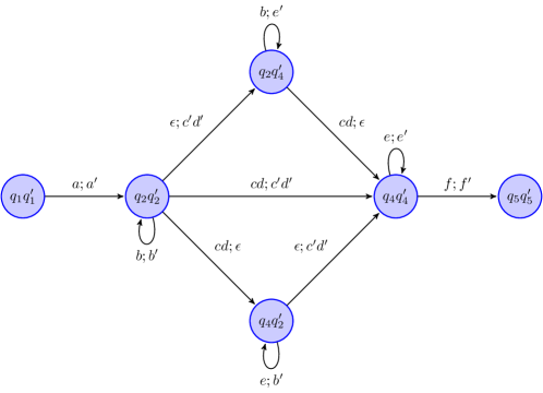
Figure 8: Directly constructed PAA for programs in Fig. 6

Case 1 corresponds to the self-loop $b;b^{\prime}$ at $q_{2}q^{\prime}_{2}$ which is included in the PAA.

Case 2a shows the predicate $i<len~{}\land~{}i^{\prime}\geq len^{\prime}$, which is not satisfiable. The reason is that the alignment predicate $i=i^{\prime}$ holds at $q_{2}q^{\prime}_{2}$ and $len=len^{\prime}$ is a loop invariant. This infeasible transition is not present in the PAA, which satisfies our requirement.

Case 2b represents the transition $q_{2}q^{\prime}_{2}\xrightarrow{\epsilon;c^{\prime}d^{\prime}}q_{2}q^{\prime}_{4}$ in our PAA. It is noteworthy that this transition is not included in the automaton from the trace-based construction (Figures 7a and 7c).

Case 3a is not a part of our PAA as well. The predicate $i\geq len~{}\land~{}i^{\prime}<len^{\prime}$ is unsatisfiable, therefore, the transition is infeasible.

Case 3b is associated with the transition $q_{2}q^{\prime}_{2}\xrightarrow{cd;\epsilon}q_{4}q^{\prime}_{2}$ in our PAA. However, this transition is not included in the trace-based automata in Figures 7a and 7b.

Cases 4a, 4b, 4c, 4d correspond to the transition $q_{2}q^{\prime}_{2}\xrightarrow{cd;c^{\prime}d^{\prime}}q_{4}q^{\prime}_{4}$, which is a part of our program alignment automaton.

It can similarly be argued that the program alignment automaton has all possible behaviours at every state. Further, notice that $i=i^{\prime}$ is an alignment predicate, which holds at each state of the PAA by construction. In particular, it holds at the exit state ($q_{5}q^{\prime}_{5}$), and thus the PAA establishes equivalence of the copies $f$ and $g$.

5 Multiple Alignment Predicates and Disjunctive Invariants

Intuitively, a PAA is good (in other words, useful in making the equivalence proof easier) if it can make the programs align at multiple locations, i.e. if there are many intermediate nodes. In the worst case, if the programs align only in the beginning, then the PAA cannot make the proof any easier (than self-composing the programs and checking).

Consider two PAAs $A$ and $A^{\prime}$ for alignment predicates $\mathcal{P}_{align}$ and $\mathcal{P^{\prime}}_{align}$ respectively. If the number of reachable nodes in $A$ is more than in $A^{\prime}$, then $A$ is considered better aligned, which certainly depends on the chosen alignment predicate. As an optimization, we can parallelize computing transitions for multiple predicates and maintain multiple transition sets. Additionally, we can discard computing transitions for the predicates that have significantly less number of reachable nodes than the other. Multiple alignment predicates can also help in suggesting disjunctive invariants. For example, consider functions $f$ and $g$ shown in Figures 9a and 9b. They take two input parameters, $h$ and $cons$, and define two local variables $y$, $z$. The function has a branching based on the value of $h$ – the first branch corresponds to the case $h>100$ while the other is taken when $h\leq 100$. Now, assume two alignment predicates: $p_{1}\mathrel{\stackrel{{\scriptstyle\scriptscriptstyle\Delta}}{{=}}}z=z^{\prime}+cons$ and $p_{2}\mathrel{\stackrel{{\scriptstyle\scriptscriptstyle\Delta}}{{=}}}y=y^{\prime}+cons$. Recall that the alignment predicate is, by assumption, true at initial state. It is easy to observe that $p_{1}$ helps in aligning first branch ($h>100$) whereas $p_{2}$ assists in the alignment of the other branch ($h\leq 100$). The predicate $p_{1}\wedge p_{2}$ fails to align either of the branches, whereas $p_{1}\vee p_{2}$ helps in aligning both the branches.

⬇

int f(int h, int cons)

{

int y = 2*h + cons;

int z = 2*h + cons;

if (h > 100) {y = 0;}

else {z = 0;}

while (h !=0) {

if (y == 0) {z--;}

else {y--;}

h--;

}

if (y == 0) {return z;}

return y;

}

a Function f

⬇

int g(int h, int cons)

{

int y = 2*h;

int z = 2*h;

if (h > 100) {y = 0;}

else {z = 0;}

while (h !=0) {

if (y == 0) {z--;}

else {y--;}

h--;

}

if (y == 0) {return (z + cons);}

return (y + cons);

}

b Function g

Figure 9: Multiple alignment predicates and their disjunction

6 Related Work

Our work is closely related to and inspired by [4], in that we also use an alignment predicate to construct a program alignment automata that semantically aligns the programs for equivalence check. However, our technique constructs the PAA directly, without needing test cases or execution traces. Our construction is similar in spirit to [7], which builds a product program without using test cases, but it requires the branching condition of one program to match that of the other. It also fails to explore many-to-many relationship among paths of component programs, which we do by constructing regular expressions and looking for suitable instantiations of them. Another technique, CoVaC [28], geared towards translation validation, constructs a cross-product of two programs to ensure that optimizing compiler transformations preserve program semantics. However, it restricts the domain of transformations such that the optimized program is consonant (structurally similar) to the source program.

Data-driven equivalence checking [25] tries to find an inductive proof of loop equivalence in the domain of compiler optimizations by inferring simulation relations based on execution traces and equality checking of the machine states. Since its goal is to align loops, the technique is not suitable for the example in Fig. 1. Other related techniques include those that prove equivalence of loop-free programs [17, 12, 11, 6, 2], or programs with finite unwindings of loops or finite input domains [23, 20, 15, 14]. There are also techniques that require some knowledge of the transformations performed [27, 18] or the order of optimizations [21, 19, 13]. In contrast, our approach can work with loops as well as in a black-box setting where knowledge about the syntactic difference in the programs is not available.

7 Conclusion and Future Work

We presented an algorithm for building program alignment automata, addressing the equivalence checking problem for two programs. Our algorithm works directly on the automaton of the individual programs, without needing any test cases or making any unrealistic assumptions. Developing a prototype tool that implements this algorithm is an immediate future work. In particular, it would be useful to explore heuristics that make the technique scale in practice. For example, by eagerly discarding states, transitions, and alignment predicates that are not leading to a good alignment automaton. An aggressive reduction of the product states may also help gain efficiency, though it may come at the cost of completeness (i.e. the PAA missing some feasible behaviors).

References

- [1] J. K. Anil, S. Prabhu, K. Madhukar, and R. Venkatesh. Using hypersafety verification for proving correctness of programming assignments. In G. Rothermel and D. Bae, editors, ICSE-NIER 2020: 42nd International Conference on Software Engineering, New Ideas and Emerging Results, Seoul, South Korea, 27 June - 19 July, 2020, pages 81–84. ACM, 2020.
- [2] T. Arons, E. Elster, L. Fix, S. Mador-Haim, M. Mishaeli, J. Shalev, E. Singerman, A. Tiemeyer, M. Y. Vardi, and L. D. Zuck. Formal verification of backward compatibility of microcode. In K. Etessami and S. K. Rajamani, editors, Computer Aided Verification, pages 185–198, Berlin, Heidelberg, 2005. Springer Berlin Heidelberg.
- [3] S. Bansal and A. Aiken. Automatic generation of peephole superoptimizers. In Proceedings of the 12th International Conference on Architectural Support for Programming Languages and Operating Systems, ASPLOS XII, page 394–403, New York, NY, USA, 2006. Association for Computing Machinery.
- [4] B. Churchill, O. Padon, R. Sharma, and A. Aiken. Semantic program alignment for equivalence checking. In Proceedings of the 40th ACM SIGPLAN Conference on Programming Language Design and Implementation, PLDI 2019, page 1027–1040, New York, NY, USA, 2019. Association for Computing Machinery.
- [5] B. Churchill, R. Sharma, J. Bastien, and A. Aiken. Sound loop superoptimization for google native client. In Proceedings of the Twenty-Second International Conference on Architectural Support for Programming Languages and Operating Systems, ASPLOS ’17, page 313–326, New York, NY, USA, 2017. Association for Computing Machinery.
- [6] D. W. Currie, A. J. Hu, and S. Rajan. Automatic formal verification of dsp software. In Proceedings of the 37th Annual Design Automation Conference, DAC ’00, page 130–135, New York, NY, USA, 2000. Association for Computing Machinery.
- [7] M. Dahiya and S. Bansal. Black-box equivalence checking across compiler optimizations. In B. E. Chang, editor, Programming Languages and Systems - 15th Asian Symposium, APLAS 2017, Suzhou, China, November 27-29, 2017, Proceedings, volume 10695 of Lecture Notes in Computer Science, pages 127–147. Springer, 2017.
- [8] A. Farzan and A. Vandikas. Automated hypersafety verification. In I. Dillig and S. Tasiran, editors, Computer Aided Verification, pages 200–218, Cham, 2019. Springer International Publishing.
- [9] G. Fedyukovich, S. J. Kaufman, and R. Bodík. Sampling invariants from frequency distributions. In 2017 Formal Methods in Computer Aided Design, FMCAD 2017, Vienna, Austria, October 2-6, 2017, pages 100–107, 2017.
- [10] G. Fedyukovich, S. Prabhu, K. Madhukar, and A. Gupta. Quantified invariants via syntax-guided synthesis. In Computer Aided Verification - 31st International Conference, CAV 2019, New York City, NY, USA, July 15-18, 2019, Proceedings, Part I, pages 259–277, 2019.
- [11] X. Feng and A. J. Hu. Automatic formal verification for scheduled vliw code. In LCTES/SCOPES ’02, 2002.
- [12] X. Feng and A. J. Hu. Cutpoints for formal equivalence verification of embedded software. In Proceedings of the 5th ACM International Conference on Embedded Software, EMSOFT ’05, page 307–316, New York, NY, USA, 2005. Association for Computing Machinery.
- [13] B. Goldberg, L. Zuck, and C. Barrett. Into the loops: Practical issues in translation validation for optimizing compilers. Electronic Notes in Theoretical Computer Science, 132(1):53 – 71, 2005. Proceedings of the 3rd International Workshop on Compiler Optimization Meets Compiler Verification (COCV 2004).
- [14] D. Jackson and D. A. Ladd. Semantic diff: a tool for summarizing the effects of modifications. Proceedings 1994 International Conference on Software Maintenance, pages 243–252, 1994.
- [15] S. K. Lahiri, C. Hawblitzel, M. Kawaguchi, and H. Rebêlo. Symdiff: A language-agnostic semantic diff tool for imperative programs. In P. Madhusudan and S. A. Seshia, editors, Computer Aided Verification, pages 712–717, Berlin, Heidelberg, 2012. Springer Berlin Heidelberg.
- [16] S. Li, X. Xiao, B. Bassett, T. Xie, and N. Tillmann. Measuring code behavioral similarity for programming and software engineering education. In Proceedings of the 38th International Conference on Software Engineering Companion, ICSE ’16, pages 501–510, New York, NY, USA, 2016. ACM.
- [17] T. Matsumoto, H. Saito, and M. Fujita. Equivalence checking of c programs by locally performing symbolic simulation on dependence graphs. In 7th International Symposium on Quality Electronic Design (ISQED’06), pages 6 pp.–375, 2006.
- [18] V. Menon, K. Pingali, and N. Mateev. Fractal symbolic analysis. ACM Trans. Program. Lang. Syst., 25(6):776–813, Nov. 2003.
- [19] G. C. Necula. Translation validation for an optimizing compiler. In Proceedings of the ACM SIGPLAN 2000 Conference on Programming Language Design and Implementation, PLDI ’00, page 83–94, New York, NY, USA, 2000. Association for Computing Machinery.
- [20] S. Person, M. B. Dwyer, S. Elbaum, and C. S. Pundefinedsundefinedreanu. Differential symbolic execution. In Proceedings of the 16th ACM SIGSOFT International Symposium on Foundations of Software Engineering, SIGSOFT ’08/FSE-16, page 226–237, New York, NY, USA, 2008. Association for Computing Machinery.
- [21] A. Pnueli, M. Siegel, and E. Singerman. Translation validation. In B. Steffen, editor, Tools and Algorithms for the Construction and Analysis of Systems, pages 151–166, Berlin, Heidelberg, 1998. Springer Berlin Heidelberg.
- [22] S. Prabhu, K. Madhukar, and R. Venkatesh. Efficiently learning safety proofs from appearance as well as behaviours. In Static Analysis - 25th International Symposium, SAS 2018, Freiburg, Germany, August 29-31, 2018, Proceedings, pages 326–343, 2018.
- [23] D. A. Ramos and D. R. Engler. Practical, low-effort equivalence verification of real code. In G. Gopalakrishnan and S. Qadeer, editors, Computer Aided Verification, pages 669–685, Berlin, Heidelberg, 2011. Springer Berlin Heidelberg.
- [24] E. Schkufza, R. Sharma, and A. Aiken. Stochastic superoptimization. In Proceedings of the Eighteenth International Conference on Architectural Support for Programming Languages and Operating Systems, ASPLOS ’13, page 305–316, New York, NY, USA, 2013. Association for Computing Machinery.
- [25] R. Sharma, E. Schkufza, B. R. Churchill, and A. Aiken. Data-driven equivalence checking. In A. L. Hosking, P. T. Eugster, and C. V. Lopes, editors, Proceedings of the 2013 ACM SIGPLAN International Conference on Object Oriented Programming Systems Languages & Applications, OOPSLA 2013, part of SPLASH 2013, Indianapolis, IN, USA, October 26-31, 2013, pages 391–406. ACM, 2013.
- [26] R. Shemer, A. Gurfinkel, S. Shoham, and Y. Vizel. Property directed self composition. In I. Dillig and S. Tasiran, editors, Computer Aided Verification, pages 161–179, Cham, 2019. Springer International Publishing.
- [27] R. Tate, M. Stepp, Z. Tatlock, and S. Lerner. Equality saturation: a new approach to optimization. In POPL ’09: Proceedings of the 36th annual ACM SIGPLAN-SIGACT symposium on Principles of Programming Languages, pages 264–276, New York, NY, USA, 2009. ACM.
- [28] A. Zaks and A. Pnueli. Covac: Compiler validation by program analysis of the cross-product. In Proceedings of the 15th International Symposium on Formal Methods, FM ’08, page 35–51, Berlin, Heidelberg, 2008. Springer-Verlag.