Length Scale Control in Topology Optimization using Fourier Enhanced Neural Networks

Abstract

Length scale control is imposed in topology optimization (TO) to make designs amenable to manufacturing and other functional requirements. Broadly, there are two types of length-scale control in TO: exact and approximate. While the former is desirable, its implementation can be difficult, and is computationally expensive. Approximate length scale control is therefore preferred, and is often sufficient for early stages of design.

In this paper we propose an approximate length scale control strategy for TO, by extending a recently proposed density-based TO formulation using neural networks (TOuNN). Specifically, we enhance TOuNN with a Fourier space projection, to control the minimum and/or maximum length scales. The proposed method does not involve additional constraints, and the sensitivity computations are automated by expressing the computations in an end-end differentiable fashion using the neural net’s library. The proposed method is illustrated through several numerical experiments for single and multi-material designs.

1 Introduction

Perhaps the most influential legacy of late Prof. Herb Voelcker is his work on the representations of solids [1]. In this paper, we investigate representing solids through a concatenation of sinusoidal functions and neural network’s activation functions, and exploiting this representation for length-scale control in topology optimization.

Topology optimization (TO) [2] is a design method which distributes material within a domain to minimize an objective function, subject to constraints. Various constraints are often imposed to make the design amenable to manufacturing and other functional requirements. One such set of constraints is to limit the maximum and minimum length scale of structural members. Imposing a maximum length $l_{max}$ will lead to desriable beam-like structures, while imposing a minimum length $l_{min}$ avoids extremely thin non-manufacturable members.

Several methods have been proposed to impose length scale control in TO (see Section 2). In this paper we propose length scale control by extending a density-based TO formulation using neural networks (TOuNN) proposed in [3], [4]. Specifically, in Section 3, we enhance TOuNN with a Fourier space projection, leading to an approximate control on both the minimum and maximum length scales. The proposed method is illustrated through numerous experiments in Section 5. Open research challenges, opportunities and conclusions are summarized in Section 6.

2 Literature Review

Popular TO methods today include density based methods ([2, 5]), level-set methods [6], and topological sensitivity methods ([7, 8, 9]). For a comprehensive review, see [10, 11]. Among these, density based methods, with solid isotropic material with penalization (SIMP) as the material model, is perhaps the most popular, and it serves as a basis for this paper.

2.1 Topology Optimization using Mesh-Based SIMP

Consider the generic TO problem illustrated in Figure 1. In density-methods, one defines a pseudo-density $\rho(\bm{x})\in(0,1]$ over the domain, where $\rho$ field is typically represented using an underlying mesh. Then, by relying on standard SIMP material penalization of the form $E=E_{0}\rho^{p}$, the field is optimized using optimality criteria [2] or MMA [12], resulting in the desired topology, as illustrated in Figure 1.

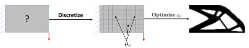
Figure 1: Classic TO using mesh-based SIMP.

Formally, the above TO problem can be posed as

$$\underset{\bm{\rho}}{\text{minimize}} \bm{u}^{\mathsf{T}}\bm{K}(\bm{\rho})\bm{u}$$ (1a)

subject to $$\bm{K}(\bm{\rho})\bm{u}=\bm{f}$$ (1b)

$$\sum_{e}\rho_{e}v_{e}\leq V^{*}$$ (1c)

where $\bm{u}$ is the displacement field, $\bm{K}$ is the finite element stiffness matrix, $\bm{f}$ is the applied force, $\rho_{e}$ is the density associated with element $e$, $v_{e}$ is the volume of the element, and $V^{*}$ is the prescribed volume.

2.2 Length Scale Control in Topology Optimization

Length-scale control , i.e., controlling feature thickness orthogonal to the local orientation, is often imposed in TO to make the design amenable to manufacturing and other functional requirements; see [13] for a review. Broadly, there are two types of length-scale control: exact and approximate.

Exact length control implies that all features must lie precisely within the length scale specified. While this may be desirable during the final stages of design, it is difficult to implement, computationally demanding and often an overkill during early stages of design. The skeletal based minimum and maximum length scale control presented in [14] is an exact length-scale strategy; practical challenges in imposing exact length-scale control were reported in this work. Further, exact length scale can contradict imposed volume fraction constraint as explained later in Section 5.4. Researchers have therefore turned towards approximate length scale control (see discussion below) since this is often sufficient for conceptual designs, AM infills, micro-structural designs, etc.

Several approximate length scale controls methods have been proposed. Filtering schemes to eliminate mesh dependency and indirectly control minimum length scale [15] is one the simplest approximate length-scale control method. In [16], a projection filter with tunable support was suggested to control the minimum length scale. However, these filters result in topologies with diffused boundaries. A scheme for imposing maximum length scale was developed in [17]. In this approach, the radius of a circular test region determines the maximum allowable member size. However, the large number of nonlinear constraints can pose challenges. Therefore, the constraints were aggregated using a p-norm form in [18, 19], within the context of infill optimization. The authors of [20] recently introduced constraints for minimum and maximum member size, minimum cavity size, and minimum separation distance. Apart from requiring a large number of elements to obtain crisp boundaries, the computation and storage of these filters can also be expensive. While most of the filters discussed above directly apply on the design variables, the readers are referred to [21] for a discussion on filtering applied to sensitivities, and to [22] for imposing manufacturing constraints using filters in TO.

Imposing approximate length scale control in the frequency domain has been suggested in [23] where a band pass filter was constructed to impose both maximum and minimum length scale controls. While this avoids additional constraints, the proposed method was restricted to rectangular domain, with non-rectangular domains requiring padding. Other techniques using morphology filters [24], geometric constraints [25] robust length scale control [26] have also been proposed. Physics-based length-scale strategies include an implicit strain energy approach [27], and a quadratic energy functional [28].

The work described in this paper relies on a Fourier projection for length-scale control. The concept of using Fourier basis functions is not new. It was first explored in [29] within a level-set formulation. It was later extended to density-methods in [23] via explicit band-pass filters that control both the minimum and maximum length scales. However, the authors noted that [23] " … it is applicable to regular rectangular domains only. Irregular domains can be extended to rectangular ones by padding the design field with zeros, which can increase the computational cost associated with the filter." This was then generalized to non-rectangular domains in [30], where the authors noted that "…[Fourier projection] decouples the geometry description, and hence the decision variables, from the finite element mesh."

In this paper, we once again use Fourier projection for length-scale control. However, instead of directly using the Fourier coefficients as design variables, a neural network (NN) is used here to control these coefficients. A few advantages of this approach are: (1) the framework can be easily extended to, say, multiple-materials, without increasing the number of design variables, (2) one can extract high resolution topology, without increasing the computational cost, and (3) one can leverage the NN’s built-in optimizer and back-propagation capabilities for automated sensitivity computations.

2.3 Topology Optimization using Neural Networks

The proposed method builds upon the TOuNN framework [3] that we briefly review. Consider once again a generic TO problem in Fig 2. As in mesh based density methods, we define a pseudo-density field $\rho$ defined at all points $(x,y)$ within the domain. However, instead of representing $\rho$ using the mesh, it is represented here using a fully-connected neural network (NN). In other words, $\rho$ is spanned by NN’s activation functions and controlled by the weights $\bm{w}$ within the NN. Then, by relying on SIMP material model, the density is optimized using the NN’s built-in optimizer to respect the imposed volume constraint $V_{c}$ , while minimizing the compliance $J$, to result in the desired topology; see Figure 2. Thus, as noted in [30], the representation scheme for the density field is independent of the mesh. However, the representational parameters, i.e., the weights, indirectly depend on the mesh, through the discrete solution to the state equation, as described in the remainder of the paper.

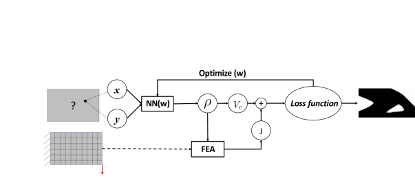
Figure 2: TOuNN framework [3].

As illustrated in Figure 3, the NN typically consists of several hidden layers (depth); each layer may consist of several activation functions such as LeakyReLU [31], [32] coupled with batch normalization [33]. By varying the height and depth, one can increase the representational capacity of the NN. The final layer is a softMax function that scales the output to values between 0 and 1.

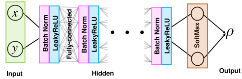
Figure 3: The architecture of the neural net in the simple TOuNN framework [3].

Formally, in TOuNN, the topology optimization problem is posed as:

$$\underset{\bm{w}}{\text{minimize}} \bm{u}^{\mathsf{T}}\bm{K}(\bm{w})\bm{u}$$ (2a)

subject to $$\bm{K}(\bm{w})\bm{u}=\bm{f}$$ (2b)

$$\sum_{e}\rho_{e}(\bm{w})v_{e}\leq V^{*}$$ (2c)

where $\bm{w}$ are the weights associated with the NN. Note that TOuNN relies on SIMP penalization of the form $E=E_{0}\rho^{p}$ to drive the density field towards 0/1.

The key characteristics of TOuNN are [3]:

1. The design variables are the NN weights $\bm{w}$.

2. The field $\rho(\bm{x})$ is infinitely differentiable everywhere in the domain.

3. The sensitivities are computed analytically using NN’s back-propagation.

4. Optimization is carried out using NN’s built-in optimizer.

3 Proposed Method

In theory, one can capture any density field in TOuNN by simply increasing the number of weights and tuning them appropriately. However, for reasons discussed in [34], standard NNs fail to efficiently capture high frequencies. This has been reported, for example, in capturing volumetric density [35], occupancy [36], signed distances[37]. Analysis shows that the eigenvalue spectrum of these networks decay rapidly as a function of frequency [38]. To alleviate this problem, projecting the input spatial coordinates to a Fourier space was proposed in [38]. With this as motivation, the proposed architecture of the Fourier enhanced NN for TO is illustrated in Figure 4.

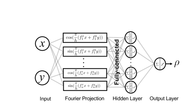
Figure 4: The architecture of the proposed neural net for 2D problems.

The critical features of the proposed Fourier-TOuNN framework are:

1. Input Layer: As before, the input to the Fourier-NN is any point $\bm{x}=(x,y)\in\mathbf{R}^{2}$ in the domain.

2. Fourier Projection Layer: This layer is the focus of the current work. The $2$ dimensional Euclidean input is transformed to a $2n_{f}$ dimensional Fourier space (see Section 3.1), where $n_{f}$ is the chosen number of frequencies. The range of frequencies is determined by the length scale controls:

   $$f\in\big{[}\frac{h}{l_{\text{max}}},\frac{h}{l_{\text{min}}}\big{]}$$ (3)

   where $h$ is the mesh edge length. Further, in this paper, the frequencies are uniformly sampled within the specified interval.

3. Hidden Layers: The output from the projected Fourier space is piped into a single layer of neurons (compared to multiple layers in Figure 3). This hidden layer is important in that it introduces an essential non-linearity. As in TOuNN, each of the neurons is associated with an activation function such as leaky-rectified linear unit (LeakyReLU), i.e., $LR^{\epsilon}(x)=max(0,x)+\epsilon min(0,x)$. Batch normalization is used for regularization.

4. Output Layer: The final layer consists of one neuron with a Sigmoid activation function, ensuring that the output density lies between 0 and 1.

In summary the output density (ignoring batch normalization) can be expressed as:

$$\rho=\frac{1}{1+exp\bigg{(}-\sum\limits_{j}w_{j}LR^{\epsilon}_{j}\big{(}\sum\limits_{i=1}^{n_{f}}w_{ij}\cos(\frac{\pi}{h}(f_{i}^{x}x+f_{i}^{y}y))+\sum\limits_{i=n_{f}}^{2n_{f}}w_{ij}\sin(\frac{\pi}{h}(f_{i}^{x}x+f_{i}^{y}y))\;\big{)}\bigg{)}}$$ (4)

where $LR^{\epsilon}_{j}$ represents the LeakyReLU operator.

3.1 A Simplified Scenario

To comprehend the transformations within the Fourier-TOuNN netowrk, consider a simplified version in Figure 5, where we limit the input dimension to 1, the frequency terms are limited to 2, and only one LeakyReLU neuron is used. The output is a single Sigmoid function as before. Then, the closed form expression for density simplifies to:

$$\rho(x)=\frac{1}{1+exp(-w_{3}LR^{\epsilon}(w_{1}\cos(\frac{\pi}{h}f_{1}^{x}x)+w_{2}\cos(\frac{\pi}{h}f_{2}^{x}x)))}$$ (5)

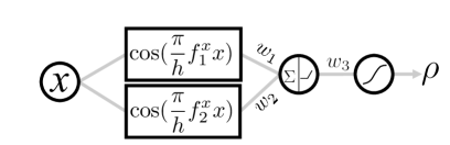
Figure 5: Simplified representation of Neural Network with Fourier Projection.

Consider an instance where $w_{1}=8$, $w_{2}=10$, $w_{3}=4$, $f_{1}^{x}=1$ and $f_{2}^{x}=6$. Figure 6 illustrates the different stages of the transformation. The plot on the top left is a simple linear combination of the two frequencies, while the plot on the top right is the output from the LeakyReLU function, which is essentially a linear transformation in the positive region, but that thresholds the negative valyes to $-\epsilon$. The Sigmoid (bottom right) further thresholds the output to $(0,1]$. The plot on the bottom left is the Fourier decomposition of the density field. As expected, the peaks are at the specified frequencies of $1$ and $6$, but spread out. This spreading of the frequencies is discussed, for example, in [38]. One can expect similar behavior in higher dimensions, and for a larger set of frequencies. Note that the Sigmoid output can be anywhere in the range $[0,1]$. However, since we use SIMP as a material model within the proposed optimization method, intermediate densities are penalized, driving the output towards 0/1 [39].

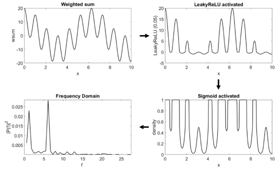
Figure 6: Different stages of transformation in a Fourier-TOuNN.

3.2 Finite Element Analysis

Although the density field is represented using the NN, a finite element mesh is needed to capture the underlying physics. Here, we use regular node quad elements, and fast Cholesky factorization based on the CVXOPT library [40]. During each iteration, the density at the center of each element is computed by the NN, and is provided to the FE solver. The FE solver computes the stiffness matrix for each element, and the assembled global stiffness matrix is then used to determine the field $\bm{u}$ and the unscaled element compliances:

$$J_{e}=\{u_{e}\}^{T}[K]_{0}\{u_{e}\}$$ (6)

The total compliance is given by:

$$J=\sum_{e}\rho_{e}^{p}J_{e}$$ (7)

where $p$ is the usual SIMP penalty parameter.

3.3 Loss Function

While many optimization methods have been proposed for use within NN (see [41]), we use the Adam optimizer [42], a gradient based optimization algorithm implemented within PyTorch. Adam optimization is designed to minimize an unconstrained loss function. In a volume constrained compliance minimization problem, it is reasonable to assume that the volume constraint in Eq. 2c is active [43] , i.e., it can be treated as an equality constraint. This would allow the use of a simple penalty method of optimization as discussed below. Towards this end, we convert the constrained minimization problem in Equation 2 into an unconstrained loss ${L}$ using a penalty formulation [44]:

$$L(\bm{w})=\frac{\sum\limits_{e}\rho_{e}^{p}J_{e}}{J_{0}}+\alpha\bigg{(}\frac{\sum\limits_{e}\rho_{e}v_{e}}{V^{*}}-1\bigg{)}^{2}$$ (8)

where $J_{0}$ is the initial compliance (for scaling), $p$ is the SIMP penalization parameter and $\alpha$ is the constraint penalty. As described in [44], starting from a small positive value for the penalty parameter $\alpha$, a gradient driven step is taken to minimize the loss function. Then, the penalty parameter is increased and the process is repeated. Observe that, in the limit $\alpha\rightarrow\infty$, when the loss function is minimized, the equality constraint is satisfied and the objective is thereby minimized.

3.4 Sensitivity Analysis

The Adam optimizer, being a first-order method, requires gradient information. In order to compute the sensitivity of the loss function (that is being minimized) with respect to the design variables, note that: (1) the design variables are the weights of the NN (instead of the element densities as in standard element-based TO), (2) the loss function comprises of the compliance and volume constraint through a penalty formulation.

With these observations, the sensitivity of the loss function with respect to any design variable $w_{i}$ is given by:

$$\frac{\partial L}{\partial w_{i}}=\sum\limits_{e}\frac{\partial L}{\partial\rho_{e}}\frac{\partial\rho_{e}}{\partial w_{i}}$$ (9)

The term $\frac{\partial\rho_{e}}{\partial w_{i}}$ is the sensitivity of element density with respect to the weights. Since the NN is nothing but a computational graph consisting of weighted sums and nonlinear activations, automatic differentiation [45] can be used to efficiently and accurately compute these terms. In particular, we utilize the automatic differentiation within PyTorch [46] in our implementation.

However, since the finite element solver is outside of the neural network, the sensitivity of compliance with respect to the density variables must be computed analytically. Thus, the sensitivity of the loss function with respect to element density, i.e., $\frac{\partial L}{\partial\rho_{e}}$, is obtained by differentiating Equation (8) and incorporating the self-adjoint term [2], resulting in:

$$\frac{\partial L}{\partial w_{i}}=\frac{-p}{J_{0}}\bigg{(}\sum_{e}\rho_{e}^{p-1}J_{e}\bigg{)}+\frac{2\alpha}{V^{*}}\bigg{(}\frac{\sum\limits_{k}\rho_{k}v_{k}}{V^{*}}-1\bigg{)}$$ (10)

The two terms are combined within the framework to compute the desired sensitivities.

3.5 Extension to Multi-Material

A key feature of the proposed framework is its versatility. Here, we show how the framework can be easily extended to multiple materials. In particular, we extend the multi-material framework proposed in [4] by adding length-scale control.

Recall from Fig. 4 that the NN for a single material had only one output neuron. To extend this to multiple materials, we simply insert additional outputs as illustrated in Fig. 7, corresponding to void $\rho^{(\phi)}$, and any of $S$ candidate materials, with corresponding mass densities $\rho^{1},\ldots\rho^{S}$. The Softmax activation of the output layer ensures that $0<\rho^{(i)}<1$. Further, the Softmax construction also ensures that the partition of unity is satisfied, i.e., $\rho^{(\phi)}+\rho^{1}+\ldots\rho^{S}=1$; please see [4] for a proof. The critical point is that one can use the same NN as was used for single material, i.e., the number of design variables remains almost unchanged, except for a few additional variables in the last layer. This is later substantiated through numerical experiments. Finally, since the computation is end-to-end differentiable, one can avoid manual sensitivity derivation. Note that, for multi-material design, a net mass constraint must be imposed instead of a volume constraint; see [4].

Figure 7: Length scale-control for multi-material TO.

4 Algorithm

The optimization procedure is summarized in Algorithm 1. We will assume that the NN has been constructed with a desired number of layers, nodes per layer and activation functions. The NN is initialized using a Glorot initializer [47]. We discretize the domain into a mesh ($\Omega^{h}$) with desired number of elements. Observe that mesh discretization is essential to capture the physics, but is not directly used to representat the density field. The coordinates of the element centers are used as inputs to the NN during optimization. The density at the center of element $e$ is denoted by $\rho_{e}$. The loss function is calculated from these discrete values. Here, we use the continuation scheme where the parameter $p$ is incremented to avoid local minima [48], [49]. The process is then repeated until termination. The algorithm is set to terminate if the percentage of gray elements (elements with densities between 0.05 and .95) $\epsilon_{g}=N_{grey}/N_{total}$ is less than a prescribed value. Here, a termination criteria of 0.0025 is used for $\epsilon_{g}$. Note that the method may not converge if the termination criteria is too small, say, less than 0.001. This is analogous to the practical termination criteria of 0.01 used in classic SIMP [50] for the density change.

A key feature of the proposed framework is that one can extract a high resolution topology at no optimization cost once the process is complete. Specifically, the optimized weights, i.e., $w^{*}$ , are used to sample the density field on a finer grid as illustrated in Fig. 8.

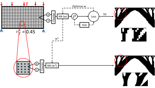
Figure 8: Extraction of high resolution topology from the NN.

Algorithm 1 Fourier-TOuNN

1:procedure TopOpt(NN, $\Omega^{h},V^{*},l_{min},l_{max}$) $\triangleright$ NN, discretized domain, desired vol, length scales

2:     $\bm{x}=\{x_{e},y_{e}\}_{e\in\Omega^{h}}$ or $\{x_{e},y_{e},z_{e}\}_{e\in\Omega^{h}}$   ; $\bm{x}\in\mathbf{R}^{n_{e}\times d}$$\triangleright$ center of elements in FE mesh; optimization input

3:     epoch = 0; $\alpha=\alpha_{0}$; $p=p_{0}$ $\triangleright$ Penalty factor initialization

4:     $J_{0}\leftarrow FEA(\bm{\rho}=v_{f}^{*},\Omega^{h})$ $\triangleright$ FEA with uniform gray

5:     $f\sim\mathcal{U}(\frac{h}{l_{max}},\frac{h}{l_{min}})$   ; $f\in\mathbf{R}^{d\times n_{f}}$ $\triangleright$ Uniformly sampled frequencies

6:     repeat$\triangleright$ Optimization

7:         $\hat{\bm{x}}=\mathcal{F}(\bm{x};f)$   ; $\hat{\bm{x}}\in\mathbf{R}^{n_{e}\times 2n_{f}}$ $\triangleright$ Project from Euclidean to Fourier

8:         $\bm{\rho}=NN(\bm{\hat{x}})$ $\triangleright$ Call NN to compute $\bm{\rho}$ at $\bm{p}$; (Forward propagation)

9:         $J_{e}\leftarrow FEA(\bm{\rho},\Omega^{h})$ $\triangleright$ Solve FEA

10:         L = $\frac{\sum\limits_{e}\rho_{e}^{p}J_{e}}{J_{0}}+\alpha\bigg{(}\frac{\sum\limits_{e}\rho_{e}v_{e}}{V^{*}}-1\bigg{)}^{2}$ $\triangleright$ Loss function

11:         Compute $\nabla L$$\triangleright$ Sensitivity(Backward Propagation)

12:         $\bm{w}\leftarrow\bm{w}+\Delta\bm{w}(\nabla L)$ $\triangleright$ Adam optimizer step

13:         $\alpha\leftarrow\text{min}(\alpha_{max},\alpha+\Delta\alpha)$ $\triangleright$ Increment $\alpha$

14:         $p\leftarrow\text{min}(p_{max},p+\Delta p)$ $\triangleright$ Continuation

15:         $\text{epoch}\leftarrow\text{epoch}+1$

16:     until  $\epsilon_{g}<\epsilon_{g}^{*}$ $\triangleright$ Check for convergence

5 Numerical Experiments

In this section, we conduct several numerical experiments to illustrate the proposed algorithm. The implementation is in Python. The default parameters are listed in Table 1. In this work, we use a continuation scheme for the SIMP penalty parameter $p$ driving it from $p=1$ at the start of optimization upto $p=8$. This ensures stability of convergence [48, 30] as well as driving the final topology to a desired 0/1 state. The minimum number of iterations is set to 150, and a maximum to 500. After optimization a grid of $15\times 15$ per element is used to extract a high resolution topology.

The total number of design variables in the proposed framework can be derived based on the following argument. Observe that $n_{f}$ cosine and sine components are passed into the projection layer. Each of the terms is fully connected to the $n_{h}$ neurons in the hidden layer. Further, each neuron in the hidden layer has a bias, and all the neurons in the hidden layer are mapped to one output neuron $(n_{o})$. Thus the total number of design variables is given by, $n_{f}*2*n_{h}+n_{h}+n_{h}*n_{o}$. In our instance, this results in a total of $150*2*20+20+20*1=6040$ design variables. The number of design variables is independent of the mesh discretization.

Parameter	Description and default value
$E$, $\nu$	Isotropic material constants Young’s Modulus (E = 1) and Poisson’s ratio ($\nu=0.3$)
$n_{f}$	Number of frequencies in projection space = 150
NN	Fully connected feed-forward network with one layer (ReLU) with 20 Neurons.
$|\bm{w}|$	The number of design variables (weight and bias) is 6040 by default
$\alpha$	Constraint penalty updated every iteration ($\alpha_{0}=\Delta\alpha=0.2$)
$p$	SIMP penalty updated every iteration ($p_{0}=1\;;\;\Delta p=0.02\;;\;p_{max}=8$)
lr	Adam Optimizer learning rate 0.01
nelx, nely	Number of mesh elements of (60, 30) along $x$ and $y$ respectively
$\epsilon_{g}^{*}$	Convergence criteria requiring fraction of gray elements be less than $\epsilon_{g}^{*}=0.0025$

Table 1: Default simulation parameters.

All experiments were conducted on an Intel i7 - 6700 CPU @ 2.6 Ghz, equipped with 16 GB of RAM. Through the experiments, we investigate the following:

1. Benchmark Studies: First we consider several TO benchmark problems, and compare the topologies obtained through mesh-based SIMP, TOuNN, and proposed Fourier-TOuNN.

2. Comparison Studies: Next, we compare the computed topologies using Fourier-TOuNN against those obtained using other length scale strategies.

3. Convergence Study: The impact of the Fourier projection on the convergence of a distributed load problem is investigated.

4. Minimum Length-Scale Control: Here, we vary the minimum length scale ($l_{min}$) and study its effect on the topology, while keeping the maximum length scale ($l_{max}$) a constant.

5. Maximum Length-Scale Control: Similarly, we will vary the maximum length scale ($l_{max}$) and study its effect on the topology, while keeping the minimum length scale ($l_{min}$) a constant.

6. Single Length-Scale Control: Next, we vary both $l_{min}$ and $l_{max}$, but keeping them equal, and study the impact on the topology.

7. Number of Frequency Samples: Next, we vary the number of frequency terms $n_{f}$ in the projected frequency space to understand its effects.

8. Depth of Neural Net: We vary the depth of NN to understand the nature of frequency spreading.

9. Multi-material design: Finally, we present an extension of the proposed work to multi-material designs.

5.1 Benchmark Studies

First we consider four benchmark topology optimization problems illustrated in the first column of Figure 9, together with the desired volume fraction. The default mesh size is $60\times 30$. The second column illustrates the topologies obtained using the popular 88-line implementation of SIMP [50], with a filter radius of 1.4, that directly controls the minimum length scale, avoiding checker-board patterns [49]; no additional length-scale control was imposed. The final compliance values and the number of finite element iterations are also listed. The third column illustrates the topologies obtained using TOuNN [3], using a neural net size of $4\times 20$ on the same mesh, without length scale control. The fourth column are the topologies obtained through the proposed Fourier-TOuNN algorithm, with $l_{min}=6$ and $l_{max}=30$. As one can observe, the topologies computed through Fourier-TOuNN exhibit thin features, and the compliance values are lower (better) than both SIMP and TOuNN. We note that the plots in the third and fourth column are at a larger resolution. This stems from the fact that, after optimization, the density values are sampled on a much finer grid (than that used for FE) to extract fine geometry as explained in Fig. 8; this comes with no additional computational cost. The total computational time for the examples in Figure 9 varied between 4-6 seconds proportional to the number of FE iterations; this is consistent with other mesh-based implementations such as [50]. Further, averaging across the examples, we observed that, in Fourier-TOuNN, FE accounts for $41\%$, forward propagation accounts for $20\%$, backward propagation accounts for $27\%$, and the remaining $13\%$ is for miscellaneous operations. This is in contrast to SIMP implementations where FE accounts for a significant portion of the computation, for instance about $96\%$ as reported in [51]. Reducing the non-FE overhead in Fourier-TOuNN via code refactoring and just-in-time compilations [52] remains to be explored.

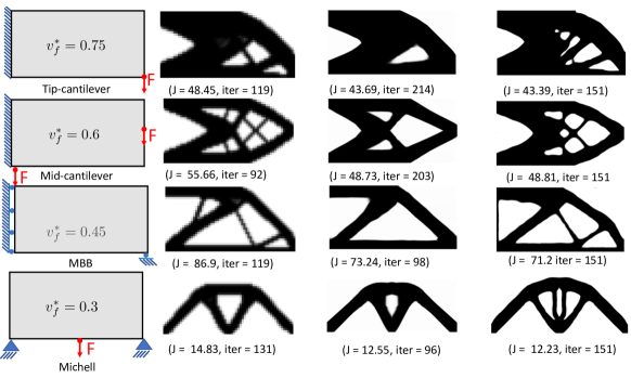
Figure 9: Comparison of topologies for various benchmark problems using SIMP [50], TOuNN [3] and proposed Fourier-TOuNN.

Next, we consider a simple tensile bar problem, (over a mesh of size $60\times 30$) as illustrated in Figure 10. The elements on the right edge are explicitly retained, while an extrude constraint along $x$ is imposed as discussed in [3]. Various length scale intervals are imposed as illustrated; the topologies and compliances obtained are consistent with expectations.

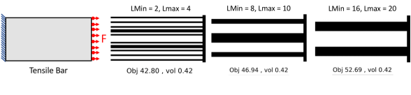
Figure 10: Tensile bar for varying length scale.

5.2 Comparison Studies

We consider the length scale results presented in [17] for a mid-cantilever beam with a mesh of $160\times 100$. With a target volume fraction of $0.5$, the minimum length scale was kept constant at $l_{min}=1$ while $l_{max}$ was varied. Figure 11 illustrates the computed topologies using the proposed method (top row) and those reported in [17] (bottom row). In both methods, as $l_{max}$ is decreased, one can observe more structural members beginning to appear. The compliance values are not compared here since it was not reported in [17].

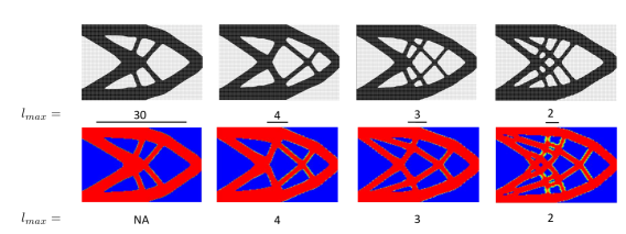
Figure 11: Benchmark comparison of designs from [17] and proposed method. The maximum length scale is decreased (left to right) with $l_{min}=2$ (NA = Not Applicable). The background grid on the top row reflects the FE mesh used.

Next we consider the results presented [53] for an MBB beam with a mesh of $300\times 100$ elements, and a desired volume fraction of $V^{*}=0.5$. The topology obtained without length scale control from [53] is illustrated in Figure 12a. Figure 12b illustrates the topology obtained through Fourier-TOuNN with a relaxed length scale control of $l_{min}=2$ and $l_{max}=150$. Figure 12 c is the reported topology [53] with a tight and equivalent length control of $l_{min}=2$ and $l_{max}=4$, while Figure 12d illustrates the Fourier-TOuNN topology with the same length control. We observe that length scale control increases the compliance as expected and more so, for exact length scale control.

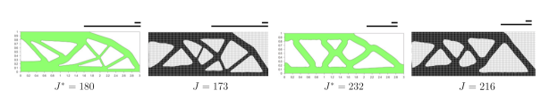
Figure 12: (a) No length scale control [53]. (b) Relaxed length scale control in Fourier-TOuNN with $l_{min}=3$ and $l_{max}=100$. (c) Tight length scale control [53] with $l_{min}=5$ and $l_{max}=8$. (d) Tight length scale control in Fourier-TOuNN with $l_{min}=5$ and $l_{max}=8$. The background grid on the top row reflects the FE mesh used.

5.3 Convergence

The distributed load problem in Figure 13 (inset) is considered next since it necessary entails thin features [54] near the loaded edge. This problem is solved using two different methods: TOuNN [3] (with no length scale control), and with the proposed Fourier-TOuNN method with length scale control ($l_{max}=30,l_{min}=4$). The elements at the top layer are retained explicitly. The difference in compliance convergence between TOuNN and Fourier-TOuNN is illustrated in Figure 13, while Figure 14 illustrates the progression of the fraction of gray elements ($\epsilon_{g}=N_{gray}/N_{total}$). We observe that TOuNN is unable to resolve the topology due to the limitations of NN. However, the proposed Fourier-TOuNN rapidly converges to a topology exhibiting thin features.

The poor convergence of TOuNN is consistent with the analysis in [38] "for a conventional NN, the eigenvalues of the Neural Tangent Kernel (NTK) decay rapidly. This results in extremely slow convergence to the high frequency components of the target function, to the point where standard NNs are effectively unable to learn these components". On the other hand, the addition of the Fourier projection leads to rapid convergence.

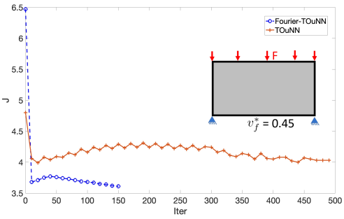
Figure 13: Convergence of compliance for distributed load at $V_{f}=0.45$ using TOuNN [3] and Fourier-TOuNN.

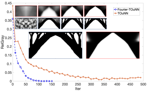
Figure 14: Progression of relative amount of gray elements for distributed load at $V_{f}=0.45$ using TOuNN [3] and Fourier-TOuNN.

5.4 Minimum Length-Scale Control

Next, we consider again the mid-cantilever beam in Figure 9, and vary $l_{min}$ between 3 and 55, while keeping $l_{max}$ constant at $l_{max}=60$. The topologies obtained using Fourier-TOuNN for various volume fractions are illustrated in Figure 15. Observe that for a given volume fraction, i.e. for each row, as $l_{min}$ is increased, the topology exhibits thicker features. Further the compliance increases (gets worse) as $l_{min}$ approaches $l_{max}$, i.e., as the solution space shrinks.

Note that a small volume fraction (first row) contradicts the large value of minimum length scale (column 4). The minimum length scale is essentially ignored by the algorithm, while the volume constraint is respected. Such contradictions can be hard to resolve in exact length scale control.

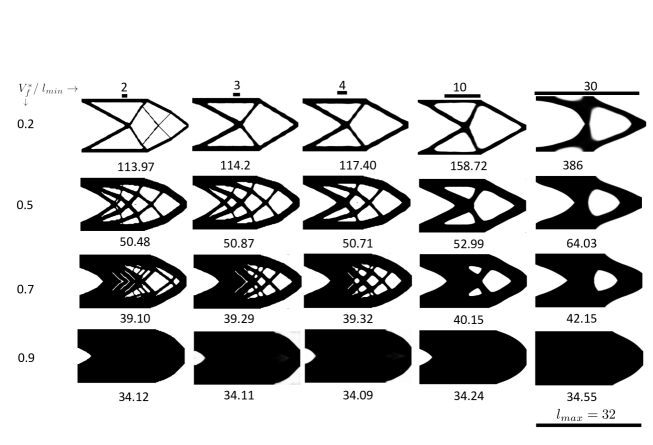
Figure 15: Varying minimum length scale with $l_{max}=60$.

5.5 Maximum Length-Scale Control

Next, we vary $l_{max}$ between 4 and 30, while keeping $l_{min}$ constant at $l_{min}=4$. The topologies obtained using Fourier-TOuNN for the mid-cantilever beam are illustrated in Figure 16 for various volume fractions. Similar to the previous experiment, for a given volume fraction, i.e., for each row, as $l_{max}$ is increased, the topologies exhibit thicker features. Further, the compliance decreases (improves) as $l_{max}$ moves away from $l_{min}$, i.e., as the solution space expands.

Once again, note that the large volume fraction imposed (last row) contradicts the small value of maximum length scale; in the current scenario, this results in disconnected topologies.

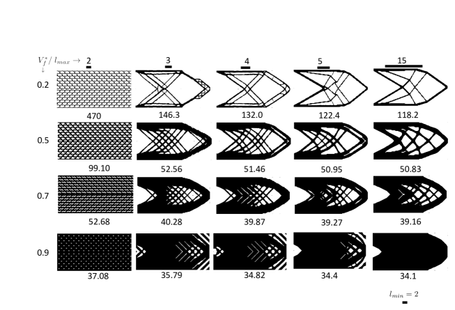
Figure 16: Varying maximum length scale with $l_{min}=4$.

5.6 Single Length-Scale Control

In the previous experiment, one can observe that, in the first column of Figure 16, when $l_{min}=l_{max}=4$, the topologies exhibit a repeated pattern. Indeed, one can obtain repeated patterns of various length scales by setting $l_{min}=l_{max}=l$. This is illustrated in Figure 17. Such patterns are often used as fillers in additive manufacturing [55, 56], and have been obtained by other researchers using various constraint techniques [18], [19], [57]. Consistent with the observations of Section 5.4 and 5.5, the imposed length scales can limit the design space, leading to sub-optimal designs.

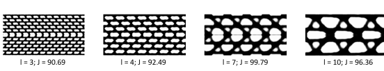
Figure 17: Repeated patterns for a mid-cantilever beam ($V_{f}=0.45$) when $l_{min}=l_{max}$.

5.7 Number of Frequency Samples

Thus far we have used a default of 150 frequency terms ($n_{f}$) within the range defined by $l_{min}$ and $l_{max}$. In this experiment, we will vary $n_{f}$ and study its effect on the topology. In particular, we consider the L-bracket problem illustrated in Figure 18. The length scales were kept constant at $l_{min}=4$ and $l_{max}=30$, and the desired volume fraction is 0.4.

Figure 18: L-Bracket with load.

The topologies obtained by varying $n_{f}$ are illustrated in Figure 19. Based on all the experiments reported in this paper, we observed that about 100 frequency terms are sufficient for convergence. Using very few frequency terms can lead to poor convergence. This is consistent with the observation made in [30] " … if too few Fourier [coefficients] are used, the resulting design is not acceptable."

Figure 19: Effect of number of frequency terms $n_{f}$ on the topology.

5.8 Depth of Neural Net

In all the experiments thus far, we have used, and recommend, a NN with just one layer. Here, we briefly consider the effect of the number of layers $n_{L}$ on the topologies for the mid-cantilever beam with $l_{min}=2\;l_{max}=20$ and $V_{f}^{*}=0.5$. From Figure 20, we observe that as we increase the depth of the NN, the topologies exhibit wiggles [30]. This observation is consistent with analysis in [38], where it was shown that additional layers can lead to frequency spreading. Thus, to limit this spread, we recommend that $n_{L}=1$, or $n_{L}=2$ in the proposed framework.

Figure 20: Effect of the NN’s depth on the topology; the number of design variables are 6040, 6460, and 7720 respectively.

5.9 Multi-material design

In this section, we demonstrate multi-material design with length scale control. Note that a mass fraction constraint must be imposed, instead of volume fraction. Therefore the physical density of all materials ($[kg\;m^{-3}]$ in $SI$) is required. For the experiments, the candidate materials are listed in Table 2, where $\lambda$ denotes the physical density. Observe that. for a given density distribution $\rho^{(i)}(x,y)$, the total mass is given by:

$$m=\sum\limits_{i=0}^{S}\int\limits_{\Omega}\lambda^{(i)}\rho^{(i)}(x,y)d\Omega$$

Index	Color	$E$	$\lambda$
$\phi$	Gray	1e-9	1e-9
1	Black	1	1
2	Red	0.8	0.7
3	Blue	0.2	0.15

Table 2: Candidate materials

For numerical demonstration, we consider again the Michell structure in Fig. 9, and impose a desired mass fraction of $0.3$, where a mass fraction of 1 means filling the entire domain with the heaviest material. The mesh size is $60\times 30$ and $n_{f}=150$.

The first experiment involves only material $\phi,1,2$ from Table 2. Figure 22 compares the computed topologies obtained using the original method (without length scale control) [4], and using the proposed framework, with $l_{min}$ = 3 and $l_{max}$ = 30. Observe that the compliance decreases with length-scale control. Compared to the single material design in Figure 9, the number of design variables increases marginally from 6040 to 6083.

Figure 21: Two multi-material designs (a) without length scale control [4] (b) with, length scale control.

Next, we repeat the experiment using all three materials $\phi,1,2,3$ from Table 2. The topologies are illustrated in Fig. 21. Observe that the volume fraction is fairly high since the light material occupies a significant portion of the design space, but the mass fraction remains at 0.3. The number of design variables increases marginally to 6104.

Figure 22: Three multi-material designs (a) without length scale control [4] (b) with, length scale control.

6 Conclusion

In this paper, we presented a simple length scale control strategy by extending the recently proposed TOuNN method [3]. The extension relied on a Fourier projection; no additional constraints were required. Further, since the computations and sensitivity analysis are performed via computational graphs and back-propagation, it is easier to compound other manufacturing constraints [58] into the framework. The optimization was performed using an Adam optimizer. Other schemes such as L-BFGS [41] may lead to faster convergence and needs further experimentation. Further, the FE solver was outside the automatic differentiation framework. Integrating a solver for end-to-end differentiation [59] will be addressed in the future. Several numerical experiments were presented to characterize the proposed method. The extension to multi-material design was also presented.

The proposed framework has several deficiencies. It only offers an approximate control over the length scales. While this may suffice certain applications, exact length scale control remains to be addressed. As observed earlier, the cost of weight updates also contributes significantly to the net computational cost. Its mitigation needs to be explored. In theory, the method can be extended to 3D, but needs to be demonstrated.

Replication of results

The Python code pertinent to this paper is available at https://github.com/UW-ERSL/Fourier-TOuNN.

Compliance with ethical standards

The authors declare that they have no conflict of interest.

References

- [1] A. A. G. Requicha and H. B. Voelcker. Solid modeling: current status and research directions. IEEE Computer Graphics and Applications, 3(7):25–37, 1983.
- [2] M P Bendsoe and Ole. Sigmund. Topology optimization: theory, methods, and applications. Springer Berlin Heidelberg, 2 edition, 2003.
- [3] Aaditya Chandrasekhar and Krishnan Suresh. TOuNN: Topology Optimization using Neural Networks. Structural and Multidisciplinary Optimization, November 2020, doi: 10.1007/s00158-020-02748-4.
- [4] Aaditya Chandrasekhar and Krishnan Suresh. Multi-material topology optimization using neural networks. Computer-Aided Design, 136:103017, 2021.
- [5] Ole Sigmund. A 99 line topology optimization code written in matlab. Structural and multidisciplinary optimization, 21(2):120–127, 2001.
- [6] J. A. Sethian and Andreas Wiegmann. Structural Boundary Design via Level Set and Immersed Interface Methods. Journal of Computational Physics, 163(2):489–528, Sep 2000.
- [7] Krishnan Suresh. A 199-line matlab code for pareto-optimal tracing in topology optimization. Structural and Multidisciplinary Optimization, 42(5):665–679, 2010.
- [8] Shiguang Deng and Krishnan Suresh. Multi-constrained topology optimization via the topological sensitivity. Structural and Multidisciplinary Optimization, 51(5):987–1001, May 2015.
- [9] Krishnan Suresh. Efficient generation of large-scale pareto-optimal topologies. Structural and Multidisciplinary Optimization, 47(1):49–61, 2013.
- [10] G. I.N. Rozvany. A critical review of established methods of structural topology optimization. Structural and Multidisciplinary Optimization, 37(3):217–237, jan 2009.
- [11] Joshua D Deaton and Ramana V Grandhi. A survey of structural and multidisciplinary continuum topology optimization: post 2000. Structural and Multidisciplinary Optimization, 49(1):1–38, 2014.
- [12] Krister Svanberg. The method of moving asymptotes—a new method for structural optimization. International journal for numerical methods in engineering, 24(2):359–373, 1987.
- [13] Boyan S. Lazarov, Fengwen Wang, and Ole Sigmund. Length scale and manufacturability in density-based topology optimization. Archive of Applied Mechanics, 86(1-2):189–218, jan 2016.
- [14] Weisheng Zhang, Wenliang Zhong, and Xu Guo. An explicit length scale control approach in SIMP-based topology optimization. Computer Methods in Applied Mechanics and Engineering, 282:71–86, dec 2014.
- [15] Ole Sigmund. On the design of compliant mechanisms using topology optimization. Journal of Structural Mechanics, 25(4):493–524, 1997.
- [16] James K Guest, Jean H Prévost, and Ted Belytschko. Achieving minimum length scale in topology optimization using nodal design variables and projection functions. International journal for numerical methods in engineering, 61(2):238–254, 2004.
- [17] James K. Guest. Imposing maximum length scale in topology optimization. Structural and Multidisciplinary Optimization, 37(5):463–473, 2009.
- [18] Jun Wu, Niels Aage, Ruediger Westermann, and Ole Sigmund. Infill Optimization for Additive Manufacturing – Approaching Bone-like Porous Structures. IEEE Transactions on Visualization and Computer Graphics, 24(2):1127–1140, 2018.
- [19] Jun Wu, Anders Clausen, and Ole Sigmund. Minimum compliance topology optimization of shell–infill composites for additive manufacturing. Computer Methods in Applied Mechanics and Engineering, 326:358–375, Nov 2017.
- [20] Eduardo Fernández, Kai ke Yang, Stijn Koppen, Pablo Alarcón, Simon Bauduin, and Pierre Duysinx. Imposing minimum and maximum member size, minimum cavity size, and minimum separation distance between solid members in topology optimization. Computer Methods in Applied Mechanics and Engineering, 368:113157, aug 2020.
- [21] Ole Sigmund and Kurt Maute. Sensitivity filtering from a continuum mechanics perspective. Structural and Multidisciplinary Optimization, 46(4):471–475, 2012.
- [22] Ole Sigmund. Manufacturing tolerant topology optimization. Acta Mechanica Sinica, 25(2):227–239, 2009.
- [23] Boyan S. Lazarov and Fengwen Wang. Maximum length scale in density based topology optimization. Computer Methods in Applied Mechanics and Engineering, 318:826–844, may 2017.
- [24] Ole Sigmund. Morphology-based black and white filters for topology optimization. Structural and Multidisciplinary Optimization, 33(4-5):401–424, apr 2007.
- [25] Mingdong Zhou, Boyan S. Lazarov, Fengwen Wang, and Ole Sigmund. Minimum length scale in topology optimization by geometric constraints. Computer Methods in Applied Mechanics and Engineering, 293:266–282, aug 2015.
- [26] M. Schevenels, B. S. Lazarov, and O. Sigmund. Robust topology optimization accounting for spatially varying manufacturing errors. Computer Methods in Applied Mechanics and Engineering, 200(49-52):3613–3627, dec 2011.
- [27] Benliang Zhu and Xianmin Zhang. A new level set method for topology optimization of distributed compliant mechanisms. International journal for numerical methods in engineering, 91(8):843–871, 2012.
- [28] Shikui Chen, Michael Yu Wang, and Ai Qun Liu. Shape feature control in structural topology optimization. Computer-Aided Design, 40(9):951–962, 2008.
- [29] Alexandra A Gomes and Afzal Suleman. Application of spectral level set methodology in topology optimization. Structural and Multidisciplinary Optimization, 31(6):430–443, 2006.
- [30] Daniel A White, Mark L Stowell, and Daniel A Tortorelli. Topological optimization of structures using fourier representations. Structural and Multidisciplinary Optimization, 58(3):1205–1220, 2018.
- [31] Ian Goodfellow, Yoshua Bengio, and Aaron Courville. Deep Learning. MIT Press, 2016.
- [32] Lu Lu, Yeonjong Shin, Yanhui Su, and George Em Karniadakis. Dying relu and initialization: Theory and numerical examples. arXiv preprint arXiv:1903.06733, 2019.
- [33] Sergey Ioffe and Christian Szegedy. Batch normalization: Accelerating deep network training by reducing internal covariate shift. In 32nd International Conference on Machine Learning, ICML 2015, volume 1, pages 448–456. International Machine Learning Society (IMLS), feb 2015.
- [34] Nasim Rahaman, Aristide Baratin, Devansh Arpit, Felix Draxlcr, Min Lin, Fred A. Hamprecht, Yoshua Bengio, and Aaron Courville. On the spectral bias of neural networks. In 36th International Conference on Machine Learning, ICML 2019, volume 2019-June, pages 9230–9239, jun 2019.
- [35] Ben Mildenhall, Pratul P Srinivasan, Matthew Tancik, Jonathan T Barron, Ravi Ramamoorthi, and Ren Ng. Nerf: Representing scenes as neural radiance fields for view synthesis. arXiv preprint arXiv:2003.08934, 2020.
- [36] Lars Mescheder, Michael Oechsle, Michael Niemeyer, Sebastian Nowozin, and Andreas Geiger. Occupancy networks: Learning 3d reconstruction in function space. In Proceedings of the IEEE Conference on Computer Vision and Pattern Recognition, pages 4460–4470, 2019.
- [37] Jeong Joon Park, Peter Florence, Julian Straub, Richard Newcombe, and Steven Lovegrove. Deepsdf: Learning continuous signed distance functions for shape representation. In Proceedings of the IEEE Conference on Computer Vision and Pattern Recognition, pages 165–174, 2019.
- [38] Matthew Tancik, Pratul P Srinivasan, Ben Mildenhall, Sara Fridovich-Keil, Nithin Raghavan, Utkarsh Singhal, Ravi Ramamoorthi, Jonathan T Barron, and Ren Ng. Fourier features let networks learn high frequency functions in low dimensional domains. arXiv preprint arXiv:2006.10739, 2020.
- [39] Yixian Du, Shuangqiao Yan, Yan Zhang, Huanghai Xie, and Qihua Tian. A modified interpolation approach for topology optimization. Acta Mechanica Solida Sinica, 28(4):420–430, 2015.
- [40] Martin S Andersen, Joachim Dahl, and Lieven Vandenberghe. Cvxopt: A python package for convex optimization. abel. ee. ucla. edu/cvxopt, 2013.
- [41] Robin M. Schmidt, Frank Schneider, and Philipp Hennig. Descending through a crowded valley — benchmarking deep learning optimizers, jul 2020.
- [42] Diederik P. Kingma and Jimmy Lei Ba. Adam: A method for stochastic optimization. In 3rd International Conference on Learning Representations, ICLR 2015 - Conference Track Proceedings. International Conference on Learning Representations, ICLR, dec 2015.
- [43] Mathias Stolpe. On some fundamental properties of structural topology optimization problems. Structural and Multidisciplinary Optimization, 41(5):661–670, 2010.
- [44] Jorge Nocedal and Stephen Wright. Numerical optimization. Springer Science & Business Media, 2006.
- [45] Atılım Günes Baydin, Barak A Pearlmutter, Alexey Andreyevich Radul, and Jeffrey Mark Siskind. Automatic differentiation in machine learning: a survey. The Journal of Machine Learning Research, 18(1):5595–5637, 2017.
- [46] Adam Paszke, Sam Gross, Francisco Massa, Adam Lerer, James Bradbury, Gregory Chanan, Trevor Killeen, Zeming Lin, Natalia Gimelshein, Luca Antiga, Alban Desmaison, Andreas Kopf, Edward Yang, Zachary DeVito, Martin Raison, Alykhan Tejani, Sasank Chilamkurthy, Benoit Steiner, Lu Fang, Junjie Bai, and Soumith Chintala. Pytorch: An imperative style, high-performance deep learning library. In Advances in Neural Information Processing Systems 32, pages 8024–8035. Curran Associates, Inc., 2019.
- [47] Xavier Glorot and Yoshua Bengio. Understanding the difficulty of training deep feedforward neural networks. In Proceedings of the thirteenth international conference on artificial intelligence and statistics, pages 249–256, 2010.
- [48] Susana Rojas-Labanda and Mathias Stolpe. Automatic penalty continuation in structural topology optimization. Structural and Multidisciplinary Optimization, 52(6):1205–1221, dec 2015.
- [49] O. Sigmund and J. Petersson. Numerical instabilities in topology optimization: A survey on procedures dealing with checkerboards, mesh-dependencies and local minima. Structural Optimization, 16(1):68–75, 1998.
- [50] Erik Andreassen, Anders Clausen, Mattias Schevenels, Boyan S. Lazarov, and Ole Sigmund. Efficient topology optimization in MATLAB using 88 lines of code. Structural and Multidisciplinary Optimization, 43(1):1–16, jan 2011.
- [51] Federico Ferrari and Ole Sigmund. A new generation 99 line matlab code for compliance topology optimization and its extension to 3d. Structural and Multidisciplinary Optimization, 62(4):2211–2228, 2020.
- [52] Siu Kwan Lam, Antoine Pitrou, and Stanley Seibert. Numba: A llvm-based python jit compiler. In Proceedings of the Second Workshop on the LLVM Compiler Infrastructure in HPC, pages 1–6, 2015.
- [53] Qi Xia and Tielin Shi. Constraints of distance from boundary to skeleton: For the control of length scale in level set based structural topology optimization. Computer Methods in Applied Mechanics and Engineering, 295:525–542, oct 2015.
- [54] Francesco Mezzadri, Vladimir Bouriakov, and Xiaoping Qian. Topology optimization of self-supporting support structures for additive manufacturing. Additive Manufacturing, 21:666–682, may 2018.
- [55] Wei Gao, Yunbo Zhang, Devarajan Ramanujan, Karthik Ramani, Yong Chen, Christopher B. Williams, Charlie C.L. Wang, Yung C. Shin, Song Zhang, and Pablo D. Zavattieri. The status, challenges, and future of additive manufacturing in engineering. Computer-Aided Design, 69:65–89, 2015.
- [56] Jikai Liu, Andrew T Gaynor, Shikui Chen, Zhan Kang, Krishnan Suresh, Akihiro Takezawa, Lei Li, Junji Kato, Jinyuan Tang, Charlie CL Wang, et al. Current and future trends in topology optimization for additive manufacturing. Structural and Multidisciplinary Optimization, 57(6):2457–2483, 2018.
- [57] Jun Wu, Charlie CL Wang, Xiaoting Zhang, and Rüdiger Westermann. Self-supporting rhombic infill structures for additive manufacturing. Computer-Aided Design, 80:32–42, 2016.
- [58] Sandro L. Vatanabe, Tiago N. Lippi, Cícero R.de Lima, Glaucio H. Paulino, and Emílio C.N. Silva. Topology optimization with manufacturing constraints: A unified projection-based approach. Advances in Engineering Software, 100:97–112, oct 2016.
- [59] Aaditya Chandrasekhar, Saketh Sridhara, and Krishnan Suresh. Auto: a framework for automatic differentiation in topology optimization. Structural and Multidisciplinary Optimization, 2021.