Distinguishability in quantum interference with multimode squeezed states

Abstract

Distinguishability theory is developed for quantum interference of the squeezed vacuum states on unitary linear interferometers. It is found that the entanglement of photon pairs over the Schmidt modes is one of the sources of distinguishability. The distinguishability is quantified by the symmetric part of the internal state of $n$ pairs of photons over the spectral Schmidt modes, whose normalization $q_{2n}$ is the probability that $2n$ photons interfere as indistinguishable. For two pairs of photons $q_{4}=(1+2\mathbb{P})/3$, where $\mathbb{P}$ is the purity of the squeezed states ($K=1/\mathbb{P}$ is the Schmidt number). For a fixed purity $\mathbb{P}$, the probability $q_{2n}$ decreases exponentially fast in $n$. For example, in the experimental Gaussian boson sampling of H.-S. Zhong et al [Science 370, 1460 (2020)], the achieved purity $\mathbb{P}\approx 0.938$ for the average number of photons $2n\geq 43$ gives $q_{2n}\lesssim 0.5$, i.e., close to the middle line between $n$ indistinguishable and $n$ distinguishable pairs of photons. In derivation of all the results the first-order quantization representation based on the particle decomposition of the Hilbert space of identical bosons serves as an indispensable tool. The approach can be applied also to the generalized (non-Gaussian) squeezed states, such as those recently generated in the three-photon parametric down-conversion.

I Introduction

Non-classical states of light are useful for the quantum information, computation and interferometry PhQI1 ; PhQI2 ; MultPhInterferom . The quantum interference of indistinguishable single photons on unitary linear multiports can serve as a basis of the computation superiority over digital computers, formulated as the boson sampling idea AA , a pathway to demonstration of the quantum advantage 20PhBS . Quantum optical platforms seem to be the most suitable for this purpose ReviewBS . One can also employ Gaussian states, instead of single photons, realizing the boson sampling with Gaussian states GBS1 ; ScattBS ; GBS2 ; ExpGBS1 ; ExpGBS2 . Gaussian states have been found useful in many other quantum information tasks GaussQI . With Gaussian states one can efficiently simulate quantum chemistry with molecules BSmolec ; MDGBS and some computational tasks on graphs Graphs1 ; Graphs2 . These tasks require scaling up the number of Gaussian states in the interference experiments, inciting the search for scalable sources ScalSQS .

Scaling up the number of interfering photons requires strong control of their distinguishability due to the fluctuating parameters. When generalizing the Hong-Ou-Mandel experiment HOM to more than two photons, it was found that the distinguishability is described by the symmetric group Ou . The effect of the distinguishability in interference with identical particles, bosons or fermions, has been studied in a number of theoretical works 3phDist ; SuffCond ; DTh ; TBonBS ; Tichy ; SYMDTh ; TL ; CollPh ; DistTimeRes ; QSPD ; SWD and experiments Dist6Ph ; 6phbunch ; genBB ; MultPh1 ; SYMDTh ; DMPI ; 4ph . Signatures of inter-species distinguishability are also revealed in systems of interacting bosons DMBD . Distinguishability degrades the quantum advantage with single photons SuffCond ; TBonBS , allowing for classical simulation of the boson sampling SimDistBS . Such a dramatic effect can also be expected with the squeezed states, used in the experiments on the Gaussian boson sampling ExpGBS1 ; ExpGBS2 . As the experimentally obtained squeezed states are multimode (i.e., the purity is not exactly $1$), one would like to know if their multi-mode structure induces partial distinguishability. Though some experiments have shown that the multi-mode structure is shaping the interference with the squeezed states ModeStrInfl , there were no clue of how one could approach such a problem.

The aim of this work is to give theory of distinguishability for interference of the squeezed vacuum states on linear unitary interferometers. The main result is the output probability distribution, applicable to the interference of an arbitrary number of multi-mode squeezed vacuum states on arbitrary linear interferometer. The four-photon interference with the multi-mode squeezed states ModeStrInfl and the output probability formula for the single-mode squeezed states GBS2 follow from the main result in these special cases. The measure of partial distinguishability, analogous to that for single photons TBonBS , is found for interference with the squeezed states. An estimate of the degree of distinguishability in the Gaussian boson sampling experiment ExpGBS2 follows. It is illuminating that all the results are easily derived by decomposing the Hilbert space of identical bosons as a direct sum of tensor powers of the single-particle Hilbert space, i.e., within the first quantization applied to identical bosons. The approach can be applied also to generalized squeezed states GenSQ , such as those obtained in the recently demonstrated three-photon parametric down-conversion 3phDC .

The rest of the text is organized as follows. In section II it is shown how to rewrite a squeezed vacuum state in the particle decomposition of the Hilbert space of identical bosons, termed here the first-order quantization representation. The relation of the latter to the oscillator decomposition in the usual, second-order, quantization, is discussed in subsection II.1. In subsection II.2 the general multi-mode squeezed states are rewritten in this form. In section III the interference of $N$ squeezed states on a unitary linear interferometer is analyzed. For the single-mode squeezed states the familiar expression for the output amplitude as a matrix Hafnian GBS2 is recovered in subsection III.1. The case of the multi-mode squeezed states with identical Schmidt modes is analyzed in subsection III.2, where we also recover, as a special case, the previous results for the four-photon interference on a beamsplitter ModeStrInfl . The case when there are orthogonal internal modes of photon pairs coming from different sources is considered in subsection III.3 and the general case is discussed in subsection III.4. In section IV a measure of the distinguishability in interference with the squeezed states is proposed and its physical interpretation is found. The partial distinguishability in the recent Gaussian boson sampling experiment of Ref. ExpGBS2 is characterized there. Possibility of application of the approach to the generalized (non-Gaussian) squeezed states is discussed in section V. Section VI gives concluding remarks. Some mathematical details, unnecessary for understanding of the main text, are placed in Appendices A-E.

II Squeezed states in the first-order quantization representation

Squeezed states ST1 ; ST2 are usually produced by the second-order nonlinearity in the process of spontaneous parametric downconversion ST3 ; ST4 ; ST5 , as well as the third-order (Kerr) nonlinearity in the four-wave mixing process ST6A ; ST6 . In the following we will consider only the squeezed vacuum states, simply referred to as the squeezed states. We will also distinguish between the degenerate and non-degenerate squeezed states, where in a degenerate squeezed state photon pairs occupy the same set of Schmidt modes (giving the spectral shape), whereas in a non-degenerate squeezed state photon pairs occupy different Schmidt modes due to different polarizations (and, possibly, also have different spectral shapes as well).

The squeezed states can be most conveniently represented by the singular-value decomposition of the squeezing Hamiltonian MMSS (see also Refs. PurityGS ; ExpMMSS ; BMR ). In general, there can be infinite number of singular values and the corresponding orthogonal (a.k.a. Schmidt) modes. The degenerate $|r)$ and non-degenerate $|\tilde{r})$ squeezed states can be always cast as follows:

$$|r)\equiv Z\exp\Biggl{\{}\frac{r}{2}\sum_{j=1}^{\infty}\sqrt{p_{j}}\hat{a}_{\phi_{j}}^{{\dagger}2}\Biggr{\}}|0),$$ (1)

$$Z=\prod_{j=1}^{\infty}\left(1-r^{2}p_{j}\right)^{\frac{1}{4}},$$

$$|\tilde{r})\equiv\tilde{Z}\exp\Biggl{\{}r\sum_{j=1}^{\infty}\sqrt{p_{j}}{\hat{a}_{H,\phi_{j}}}^{\dagger}{\hat{a}_{V,\psi_{j}}}^{\dagger}\Biggr{\}}|0),$$ (2)

$$\tilde{Z}=\prod_{j=1}^{\infty}\left(1-r^{2}p_{j}\right)^{\frac{1}{2}},$$

where $\hat{a}_{\phi_{j}}^{\dagger}$ is the photon creation operator for Schmidt mode $\phi_{j}$ and, similarly, ${\hat{a}_{H,\phi_{j}}}^{\dagger}$, ${\hat{a}_{V,\psi_{j}}}^{\dagger}$, with $H,V$ denoting two orthogonal polarizations and $j$ generally different spectral modes, $\phi_{j}$ for $V$ and $\psi_{j}$ for $H$, whereas $|0)$ denotes the vacuum state (the tensor product of the vacuum states in all the modes). The polarization is omitted in the degenerate case for simplicity. Here and below the notation $|\ldots)$ is used for the Fock states and squeezed states, whereas the standard notation $|\ldots\rangle$ is reserved for the states in the first-order quantization representation (see details in section II.1). The singular-values $0\leq p_{j}\leq 1$ are conveniently normalized, where $\sum_{j=1}^{\infty}p_{j}=1$ (this choice will become clear below), whereas the normalization factor $0<r<1$ (we consider $r$ to be real as the possible phase factor can be incorporated into the boson creation operators) will be called the squeezing parameter ($r=\tanh\kappa$, where $\kappa$ is usually called the squeezing parameter). For a single-mode squeezed state ($p_{1}=1$) the parameter $r$ in Eqs. (1)-(2) is related to the average number of detected photons $2\bar{n}$ as follows $2\bar{n}=r^{2}/(1-r^{2})$ (i.e., $2\bar{n}=\sinh^{2}\kappa$). The set of singular-values $\{p_{1},p_{2},\ldots\}$ characterizes multimodeness of the squeezed state, which can be quantified either by the purity $0<\mathbb{P}\leq 1$ or by the Schmidt number $1\leq K<\infty$ MMSS ; PurityGS ; ExpMMSS ; BMR ; ModeStrInfl , where

$$\mathbb{P}=\sum_{j=1}^{\infty}p_{j}^{2},\quad K=\frac{1}{\mathbb{P}}.$$ (3)

The Schmidt number was recently shown to shape the four-photon interference ModeStrInfl .

In Eqs. (1)-(2) we have tacitly assumed that the squeezed states are pure states, i.e., that there is perfect cross-photon-number coherence, which is sometimes argued to be unnecessary for understanding the experiments PhNumIn ; noSS . The squeezed states in Eqs. (1)-(2) represent the usual parametric approximation, applicable when the pump is sufficiently strong and the interaction times are sufficiently short PumpEff . This approximation disregards the precise balance of annihilated and created photons due to the energy conservation SPent ; EnConDC . Taking such a balance into account would result in imperfect coherence between the multi-photon components with different $n$, due to entanglement with generally different quantum states of the pump. Here, we disregard such effects, relegating their study to future publications.

Below, we will derive another, more useful for our purposes, representation of the squeezed states. Our representation utilizes another possible decomposition of the Hilbert space of identical bosons, in contrast to the standard decomposition by independent oscillators. The relation between the two is discussed below.

II.1 The first-order and second-order quantization representations for identical bosons

The quantization of the electromagnetic field, historically termed the second quantization, is usually performed by representing it as a system of independent oscillators in some orthogonal modes. In this approach the Hilbert space of quantum states of photons is decomposed as the tensor product of the Hilbert spaces of independent oscillators.

The term first quantization refers to quantum description of particles, such as a system of identical bosons. In this approach the symmetric subspace of the tensor power of the Hilbert space of individual bosons is the physical Hilbert space (in general, it is the direct sum of such subspaces, when the number of bosons is not fixed).

Photons are bosons, hence there is a mathematical equivalence between the above two approaches. Below this mathematical equivalence is exposed following Ref. MyNotes (similar approach is used in Quantum Statistical Mechanics by Bogolubov BogBog and the essential features are found already in Dirac Dirac ). We will use the terms “second-order quantization” and ‘first-order quantization” referring to the above two decompositions of the Hilbert space of identical bosons.

In the first-order quantization approach $n$ identical bosons occupy a completely symmetric state in the tensor power space $\mathcal{H}^{\otimes n}$, where $\mathcal{H}$ is the Hilbert space of a single boson (i.e., of the single-particle states). If the occupied single-particle states are some orthogonal states $|\psi_{k}\rangle\in\mathcal{H}$, $k=1,2,\ldots$, with occupations, say, $\mathbf{n}=(n_{1},n_{2},\ldots,n_{m})$, $|\mathbf{n}|=n_{1}+n_{2}+\ldots+n_{m}=n$ (and the rest $n_{j}=0$), then the state of $n$ bosons in $\mathcal{H}^{\otimes n}$ in $m$ modes is the following Fock state

$$|n_{1},n_{2},\ldots,n_{m})^{(I)}\equiv\sqrt{\frac{n!}{\mathbf{n}!}}\hat{S}_{n}|\psi_{k_{1}}\rangle\ldots|\psi_{k_{n}}\rangle$$

$$\qquad=\sqrt{\frac{n!}{\mathbf{n}!}}\hat{S}_{n}|\psi_{1}\rangle^{\otimes n_{1}}\dots|\psi_{m}\rangle^{\otimes n_{m}},$$ (4)

where $k_{1},k_{2},\ldots,k_{n}$ is the multi-set of indices corresponding to the non-zero occupations $\mathbf{n}$, $\mathbf{n}!=n_{1}!n_{2}!\ldots n_{m}!$, and $\hat{S}_{n}$ is the projector on the symmetric subspace of $\mathcal{H}^{\otimes n}$ defined as follows:

$$\hat{S}_{n}=\frac{1}{n!}\sum_{\sigma\in S_{n}}\hat{P}_{\sigma},$$ (5)

$$\hat{P}_{\sigma}|\phi_{1}\rangle|\phi_{2}\rangle\ldots|\phi_{n}\rangle\equiv|\phi_{\sigma^{-1}(1)}\rangle|\phi_{\sigma^{-1}(2)}\rangle\ldots|\phi_{\sigma^{-1}(n)}\rangle,$$

where $\sigma$ is an element (permutation) of the symmetric group $S_{n}$ of $n$ objects. Due to the group property, $\hat{P}_{\sigma}\hat{P}_{\tau}=\hat{P}_{\sigma\tau}$, we have $\hat{P}_{\sigma}\hat{S}_{n}=\hat{S}_{n}$ and $\hat{S}^{2}_{n}=\hat{S}_{n}$, thus $\hat{S}_{n}$ is a projector on the symmetric subspace of the tensor power of $\mathcal{H}^{\otimes n}$, denoted below $\hat{S}_{n}\left\{\mathcal{H}^{\otimes n}\right\}$. More generally, when $n$ bosons occupy some arbitrary single-particle states $|f_{1}\rangle,\ldots,|f_{n}\rangle\in\mathcal{H}$, then the following unnormalized state

$$|f_{1},\ldots,f_{n}\rangle\equiv\hat{S}_{n}|f_{1}\rangle\ldots|f_{n}\rangle$$ (6)

corresponds to this case. The normalization factor for the state in Eq. (6) can be derived from the inner product of two symmetric states, which reads

$$\langle g_{1},\ldots,g_{n}|f_{1},\ldots,f_{n}\rangle=\frac{1}{n!}\sum_{\sigma}\prod_{i=1}^{n}\langle g_{i}|f_{\sigma(i)}\rangle.$$ (7)

Any state of $n$ bosons is also some linear combination of Fock states, as in Eq. (II.1), in any given basis in $\mathcal{H}$. Thus, the state in Eq. (6) can be rewritten as such by expansion of the single-particle states $|f_{k}\rangle$ in a given basis.

The equivalence between the first-order and second-order quantization of identical bosons can be established by introducing the equivalents of the boson creation and annihilation operators as some linear operators acting between the symmetric subspaces $\hat{S}_{n}\left\{\mathcal{H}^{\otimes n}\right\}$ with different $n$. Consider the following two operators MyNotes :

$$\hat{A}^{+}_{\phi}|f_{1},\ldots,f_{n}\rangle\equiv\sqrt{n+1}\hat{S}_{n+1}|\phi\rangle|f_{1},\ldots,f_{n}\rangle,$$

$$\hat{A}^{-}_{\phi}|f_{1},\ldots,f_{n}\rangle\equiv\sqrt{n}(\langle\phi|\otimes I\otimes\ldots\otimes I)|f_{1},\ldots,f_{n}\rangle$$

$$\quad=\frac{1}{\sqrt{n}}\sum_{i=1}^{n}\langle\phi|f_{i}\rangle|f_{1},\ldots,f_{i-1},f_{i+1},\ldots,f_{n}\rangle,$$ (8)

where for $\hat{A}^{-}_{\phi}$ we have used the expansion $S_{n}=\sum_{i=1}^{n}(1,i)S^{(i)}_{n-1}$, with $(1,i)$ being the transposition of $1$ and $i$ (fixed point for $i=1$) and $S^{(i)}_{n-1}$ the symmetric group of permutations of $(1,2,\ldots,i-1,i+1,\ldots,n)$. By definition, the operator $\hat{A}^{+}_{\phi}$ acts by adding a boson in the state $|\phi\rangle$ to the state it applies to (and symmetrization), whereas, the operator $\hat{A}^{-}_{\phi}$ acts by removing a boson in the state $|\phi\rangle$ (replacing a single-particle state by the amplitude of its projection on $|\phi\rangle$). One can show MyNotes that the introduced operators satisfy the following properties:

$$(\hat{A}^{\pm}_{\phi})^{\dagger}=\hat{A}^{\mp}_{\phi},$$

$$[\hat{A}^{\pm}_{\psi},\hat{A}^{\pm}_{\phi}]=0,$$

$$[\hat{A}^{-}_{\psi},\hat{A}^{+}_{\phi}]=\langle\psi|\phi\rangle,$$ (9)

where $[\hat{A},\hat{B}]=\hat{A}\hat{B}-\hat{B}\hat{A}$ is the commutator. For a basis $|\psi_{k}\rangle$, $k=1,2,\ldots,$ in $\mathcal{H}$, we recover the usual commutation relations for the boson creation and annihilation operators by associating

$$\hat{a}^{\dagger}_{\psi_{k}}=\hat{A}^{+}_{\psi_{k}},\quad\hat{a}_{\psi_{k}}=\hat{A}^{-}_{\psi_{k}}.$$ (10)

The final step is to complete the sequence of the tensor powers $\mathcal{H}^{\otimes n}$ to that with $n\geq 0$ by adding the $0$-power $\mathcal{H}^{\otimes 0}\equiv\{|\;\rangle\}$ (i.e., the state containing no particles; see also Ref. Dirac ) by postulating $|\;\rangle\equiv|0)$, where $|0)\equiv\prod_{k}|0)_{k}$ is the tensor product of the individual vacuum states $|0)_{k}$ of all modes in some basis. Then, a repeated application of the definition of the creation operator in Eq. (8) to the vacuum state gives

$$\hat{a}^{\dagger}_{\phi_{1}}\ldots\hat{a}^{\dagger}_{\phi_{n}}|0)=\sqrt{n!}\hat{S}_{n}|\phi_{1}\rangle|\phi_{2}\rangle\ldots|\phi_{n}\rangle,$$ (11)

where the boson operators $\hat{a}^{\dagger}_{\phi_{1}},\ldots,\hat{a}^{\dagger}_{\phi_{n}}$ create arbitrary (i.e., non-orthogonal, in general) single-particle states $|\phi_{1}\rangle,\ldots,|\phi_{n}\rangle\in\mathcal{H}$. For example, Eq. (11) relates the Fock state of $n$ bosons in $m$ modes in the second-order quantization representation and its equivalent Fock state in the first-order quantization representation, Eq. (II.1), Dirac :

$$|n_{1},n_{2},\ldots,n_{m})^{(II)}\equiv\frac{(\hat{a}^{\dagger}_{\psi_{1}})^{n_{1}}\ldots(\hat{a}^{\dagger}_{\psi_{m}})^{n_{m}}}{\sqrt{\mathbf{n}!}}|0)$$ (12)

$$=\sqrt{\frac{n!}{\mathbf{n}!}}\hat{S}_{n}|\psi_{1}\rangle^{\otimes n_{1}}\dots|\psi_{m}\rangle^{\otimes n_{m}}=|n_{1},n_{2},\ldots,n_{m})^{(I)},$$

where $\mathbf{n}=(n_{1},n_{2},\ldots,n_{m})$, $|\mathbf{n}|\equiv n_{1}+n_{2}+\ldots+n_{m}=n$. The oscillator modes themselves form a basis of the Hilbert space of single-partile states $\mathcal{H}$.

In summary, the Hilbert space of identical bosons $\mathscr{H}$ in the second-order quantization representation is the tensor product of the Hilbert spaces $H_{k}$ of the orthogonal oscillators in a basis of modes $|\psi_{k}\rangle\in\mathcal{H}$, whereas in the first-order quantization representation it is a direct sum of the symmetric subspaces of the tensor powers of the Hilbert space $\mathcal{H}$ of individual bosons:

$$\mathscr{H}=\prod_{k=1}^{\mathrm{dim}\mathcal{H}}\!{}^{\otimes}H_{k}=\sum_{n=0}^{\infty}{\!}^{\oplus}\hat{S}_{n}\left\{\mathcal{H}^{\otimes n}\right\},$$ (13)

where $\hat{S}_{0}=\openone$. The action of the boson creation and annihilation operators for a given basis of modes can be represented schematically as follows:

$$H_{k}\xrightarrow{\hat{a}^{\dagger}_{\psi_{k}},\hat{a}_{\psi_{k}}}H_{k},$$

$$\hat{S}_{n}\left\{\mathcal{H}^{\otimes n}\right\}\xrightarrow{\hat{a}^{\dagger}_{\psi_{k}}}\hat{S}_{n+1}\left\{\mathcal{H}^{\otimes(n+1)}\right\},$$

$$\hat{S}_{n}\left\{\mathcal{H}^{\otimes n}\right\}\xrightarrow{\hat{a}_{\psi_{k}}}\hat{S}_{n-1}\left\{\mathcal{H}^{\otimes(n-1)}\right\},$$ (14)

where in the last line $n\geq 1$, whereas for $n=0$ we have $\hat{S}_{0}\left\{\mathcal{H}^{\otimes 0}\right\}\xrightarrow{\hat{a}_{\psi_{k}}}0$.

Finally, below we will also utilize a factorization of the oscillator modes, such as the Schmidt modes in Eq. (1)-(2), into the spatial mode, below denoted simply by $|k\rangle$, $k=1,\ldots,M$, and corresponding to input port of an unitary interferometer the squeezed state is launched to (this nomenclature will include also the polarization, fixed in the degenerate case, but also in the non-degenerate case, see section III) and the internal states $|\phi^{(k)}_{j}\rangle$, $j\geq 1$. In this case the single-particle state becomes the product of such states (corresponding to different degrees of freedom of a photon), e.g., in the case of the degenerate squeezed state launched into input port $k$ of the interferometer, the single-particle states become $|k\rangle|\phi^{(k)}_{j}\rangle\in\mathcal{H}$. Thus, two-index (sometimes three-index) notation for the creation and annihilation operators will be used (the third index giving the polarization).

II.1.1 Linearity of the boson operators $\hat{A}^{\pm}$

Note that by the definition the Fock space operator $\hat{A}^{+}_{\phi}$ is linear in the state it “creates”:

$$|\phi\rangle=a|f\rangle+b|g\rangle\quad\Rightarrow\quad\hat{A}^{+}_{\phi}=a\hat{A}^{+}_{f}+b\hat{A}^{+}_{g}.$$ (15)

The importance of this property in linear optics can be now appreciated. If the Hilbert space $\mathcal{H}$ has a finite dimension $M$, e.g., as for an interferometer, the change of the basis $|\psi_{k}\rangle\to|\phi_{k}\rangle$, $k=1,\ldots,M$, by some unitary matrix $U$,

$$|\psi_{k}\rangle=\sum_{k=1}^{M}U_{kl}|\phi_{l}\rangle,$$ (16)

induces the respective transformation for the operators. Indeed, by the linearity property in Eq. (15), the corresponding transformation of the creation operators is

$$\hat{a}^{\dagger}_{\psi_{k}}=\sum_{k=1}^{M}U_{kl}\hat{a}^{\dagger}_{\phi_{l}},\quad\hat{a}^{\dagger}_{\phi_{l}}\equiv\hat{A}^{+}_{\phi_{l}}.$$ (17)

The linear transformation in Eq. (16) is the result of the unitary evolution

$$\hat{a}^{\dagger}_{\phi_{k}}=\hat{U}^{\dagger}\hat{a}^{\dagger}_{\psi_{k}}\hat{U},\quad\hat{U}\equiv\exp\left\{i\sum_{k,l=1}^{M}\hat{a}^{\dagger}_{\psi_{k}}E_{lk}\hat{a}_{\psi_{l}}\right\},$$ (18)

where the Hermitian matrix $E$ is obtained from the exponent of the matrix $U$: $U=e^{iE}$. Observe that in Eq. (16) and its consequence (17) the words “linear optical operation” have clear physical interpretation: the single-particle states (the states in $\mathcal{H}$) for each boson in a multi-boson state are simply expanded in another basis.

One comment on the usage of Eq. (11) is in order. The projector $\hat{S}_{n}$ on the r.h.s. of Eq. (11) depends on the total number of bosons, i.e., the factorization by mode property of the oscillator decomposition of the Hilbert space has no equivalent in the particle decomposition. For example, Eq. (11) cannot be used to get an equivalent first-order quantization representation of a single-mode Fock state $|n)_{k}\equiv\left(\hat{a}^{\dagger}_{\psi_{k}}\right)^{n}|0)_{k}$, where $|0)_{k}\in H_{k}$ but $|0)_{k}\notin\mathscr{H}$ (when there are other oscillator modes). The common vacuum $|0)=\prod_{k}|0)_{k}\in\mathscr{H}$ should be used in Eq. (11), which relates the above two decompositions of the whole Hilbert space $\mathscr{H}$ of identical bosons. Note that it does not matter which orthogonal basis of modes in the Hilbert space $\mathcal{H}$ is used for the mode factorization of the common vacuum state $|0)$, since any linear evolution, Eqs. (17)-(18), leaves it invariant.

The first-order quantization representation can be used to simplify calculations of the quantum probabilities of photon detection at output of a linear interferometer, since it allows the decomposition the photon degrees of freedom into two classes SuffCond ; DTh : the operating modes affected by interferometer according to Eqs. (16)-(17) and the internal states (or modes) which are invariant under the action of the interferometer.

II.2 Squeezed vacuum states in the first-order quantization representation

Let us find the first-order quantization representation of the squeezed states of Eqs. (1)-(2). Consider first the degenerate case. It can be viewed as the tensor product of the single-mode squeezed states, indexed by $j$ in Eq. (1), and having the squeezing parameters $r_{j}=r\sqrt{p_{j}}$. Introduce $\mathbf{n}=(n_{1},n_{2},\ldots)$, where $2\mathbf{n}$ is the vector of Fock occupation numbers of the Schmidt modes. We will use the following identity between the summation over the occupations $\mathbf{n}$ and the product of independent summations over the Schmidt modes,

$$\sum_{|\mathbf{n}|=n}f(\mathbf{n})=\sum_{j_{1}=1}^{\infty}\ldots\sum_{j_{n}=1}^{\infty}\frac{\prod\limits_{j=1}^{\infty}n_{j}!}{n!}f(\mathbf{n}),$$ (19)

valid for an arbitrary function $f(\mathbf{n})$ of the occupations. Using the identity of Eq. (19) we obtain

$$|r)=\prod_{j=1}^{\infty}|r_{j})=Z\sum_{\mathbf{n}}\prod_{j=1}^{\infty}\left(\frac{r_{j}}{2}\right)^{n_{j}}\frac{(\hat{a}_{\phi_{j}}^{\dagger})^{2n_{j}}}{n_{j}!}|0)$$

$$=Z\sum_{n=0}^{\infty}\frac{1}{n!}\sum_{j_{1}=1}^{\infty}\ldots\sum_{j_{n}=1}^{\infty}\prod_{\alpha=1}^{n}\frac{r_{j_{\alpha}}}{2}\hat{a}_{\phi_{j_{\alpha}}}^{{\dagger}2}|0)$$

$$=Z\sum_{n=0}^{\infty}\binom{2n}{n}^{\frac{1}{2}}\sum_{j_{1}=1}^{\infty}\ldots\sum_{j_{n}=1}^{\infty}\prod_{\alpha=1}^{n}\frac{r_{j_{\alpha}}}{2}$$

$$\times\hat{S}_{2n}|\phi_{j_{1}}\rangle|\phi_{j_{1}}\rangle\ldots|\phi_{j_{n}}\rangle|\phi_{j_{n}}\rangle$$

$$=Z\sum_{n=0}^{\infty}\binom{2n}{n}^{\frac{1}{2}}\hat{S}_{2n}\Biggl{(}\frac{r}{2}\sum_{j=1}^{\infty}\sqrt{p_{j}}|\phi_{j}\rangle|\phi_{j}\rangle\Biggr{)}^{\!\!\otimes n},$$ (20)

where we have introduced the Schmidt mode $\phi_{j}$, such that $|\phi_{j}\rangle=\hat{a}^{\dagger}_{\phi_{j}}|0)$, and used Eq. (11) for the first-order quantization representation of the $2n$-photon state,

$$\prod_{\alpha=1}^{n}\hat{a}_{\phi_{j_{\alpha}}}^{{\dagger}2}|0)=\sqrt{(2n)!}\hat{S}_{2n}\prod_{\alpha=1}^{n}|\phi_{j_{\alpha}}\rangle^{\otimes 2}.$$ (21)

Quite similarly, we get the first-order quantization representation of the non-degenerate squeezed vacuum state

$$|\tilde{r})=\prod_{j=1}^{\infty}|r_{j})={Z}\sum_{\mathbf{n}}\prod_{j=1}^{\infty}{r_{j}}^{n_{j}}\frac{\left(\hat{a}_{H,\phi_{j}}^{\dagger}\hat{a}_{V,\psi_{j}}^{\dagger}\right)^{n_{j}}}{n_{j}!}|0)$$

$$={\tilde{Z}}\sum_{n=0}^{\infty}\binom{2n}{n}^{\frac{1}{2}}\hat{S}_{2n}\Biggl{(}r\sum_{j=1}^{\infty}\sqrt{p_{j}}|H,\phi_{j}\rangle|V,\psi_{j}\rangle\Biggr{)}^{\!\!\otimes n},$$

where $|H,\phi_{j}\rangle=|H\rangle|\phi_{j}\rangle=\hat{a}_{H,\phi_{j}}^{\dagger}|0)$ and $|V,\psi_{j}\rangle=|V\rangle|\psi_{j}\rangle=\hat{a}_{V,\psi_{j}}^{\dagger}|0)$.

Above we have used a simplified nomenclature, omitting the spatial mode index (indicating the input port of an interferometer where the squeezed state is launched), since we have considered a single such multimode squeezed state. Below, therefore, we will have to add another index to the boson operators, indicating the input port where the state is launched, e.g., $|k\rangle|\phi_{j}\rangle=\hat{a}^{\dagger}_{k,\phi_{j}}|0)$ and $|k\rangle|H\rangle|\phi_{j}\rangle=\hat{a}^{\dagger}_{k,H,\phi_{j}}|0)$, etc, where we have denoted by index $k$ the spatial mode corresponding to interferometer input port $k$. To avoid the confusion with the input port operators, will use the notation $\hat{b}^{\dagger}_{l,\phi_{j}}|0)=|l^{(out)}\rangle|\phi_{j}\rangle$, etc, for the boson creation operators in the spatial output port $l$ of an interferometer.

One can convert a non-degenerate single-mode squeezed state into two degenerate single-mode squeezed states in two different spatial modes by a unitary transformation. Such a transformation can be physically realized by first separating the polarizations into two spatial modes by the polarizing beamsplitter, changing one of the polarizations by a wave plate and using a balanced beamsplitter on the output modes. The effect on the two boson operators, say $\hat{a}_{1,H}^{\dagger}$ and $\hat{a}_{1,V}^{\dagger}$, in the non-degenerate squeezed state of the same spatial mode can be accounted for by the following unitary transformation

$$\left(\begin{array}[]{c}\hat{a}_{1,H}^{\dagger}\\ \hat{a}_{1,V}^{\dagger}\end{array}\right)=\left(\begin{array}[]{cc}\frac{1}{\sqrt{2}}&\frac{i}{\sqrt{2}}\\ \frac{1}{\sqrt{2}}&\frac{-i}{\sqrt{2}}\end{array}\right)\left(\begin{array}[]{c}\hat{b}_{1,V}^{\dagger}\\ \hat{b}_{1,V}^{\dagger}\end{array}\right),$$ (23)

which will be called below the polarization-to-propagation mode beamsplitter, where $\hat{b}_{1,V}^{\dagger},\hat{b}_{2,V}^{\dagger}$ describe two output spatial modes of the same polarization. The product of two boson operators in the exponent of a non-degenerate squeezed state transforms as follows

$$\hat{a}_{1,H}^{\dagger}\hat{a}_{1,V}^{\dagger}=\frac{1}{2}\left(\hat{b}_{1,V}^{{\dagger}2}+\hat{b}_{2,V}^{{\dagger}2}\right).$$ (24)

We have seen above that a two-mode squeezed state in two different polarizations becomes a product of two single-mode squeezed states in another basis (which requires using an interferometer). A two-mode squeezed state can always be represented as a product of two single-mode squeezed states Milburn . This is a particular case of the so-called Bloch-Messiah reduction BMRed : a Gaussian unitary acting on the vacuum state can always be represented as a product of single-mode squeezers in a properly chosen modal basis. The physical setup for such a mathematical transformation necessitates using an interferometer. The multi-mode squeezed states in Eqs. (1)-(2) are tensor products of the single-mode states over the Schmidt modes. However, the spectral Schmidt modes are not affected by spatial interferometers MMSS ; PurityGS ; ExpMMSS ; ModeStrInfl ; BMR . Therefore, despite the existence of a formal mathematical equivalence, the multimode squeezed states at input of a spatial interferometer are not equivalent to the single-mode squeezed states at input of any other spatial interferometer. The multimode structure of such squeezed states affects the interference of them on spatial interferometers, as demonstrated already in Ref. ModeStrInfl . Moreover, as we will see below, the spectral Schmidt modes affect interference of the squeezed states in a similar way as the mixed internal states of single photons do. Therefore, in accordance with terminology used for single photons 3phDist ; SuffCond ; DTh ; TBonBS ; Tichy ; SYMDTh ; TL ; CollPh ; DistTimeRes ; QSPD ; SWD , the spectral Schmidt modes will be called below the internal modes. In Eqs. (II.2) and (II.2) the internal modes are the states $|\phi_{j}\rangle$ and $|\psi_{j}\rangle$. Observe also that degenerate and non-degenerate squeezed states are not always equivalent in quantum interference experiments. The non-degenerate squeezed state of Eq. (II.2) may have different internal modes for different polarizations ($|\phi\rangle\neq|\psi\rangle$), unlike the degenerate squeezed state of Eq. (II.2). Such states cannot be transformed into one another by a spatial interferometer, since the unitary transformation Milburn ; BMRed relating them has to act on the internal modes (e.g., in this case we would have the product $\hat{a}_{1,H,\phi}^{\dagger}\hat{a}_{1,V,\psi}^{\dagger}$ on the l.h.s. of Eq. (24), with the internal modes $|\phi\rangle\neq|\psi\rangle$, and no linear unitary transformation not affecting the internal modes would transform such a product into the sum of two operators squared).

III Output probability from interference of squeezed states

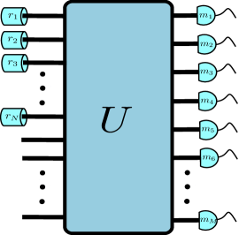
Figure 1: A schematic depiction of the considered setup. Here $N$ degenerate squeezed vacuum states with squeezing parameters $r_{1},\ldots,r_{N}$ are launched at the input of a linear $M$-port interferometer given by a unitary matrix $U$. At the output $M$ particle number resolving detectors give a configuration $m_{1},\ldots,m_{M}$, with $m_{l}$ particles detected at output port $l$. In the non-degenerate case, the two polarization modes from squeezed source $k$ are assumed to be launched into inputs $k$ and $N+k$.

We will consider quantum interference of $N$ multimode squeezed vacuum states having the overall squeezing parameters $r_{1},\ldots,r_{N}$, and impinging on an $M$-port interferometer, represented here by a unitary matrix $U$ (schematically depicted in Fig. 1). In the non-degenerate case we assume that photons of different polarizations are allowed to interfere (e.g., by using the polarizing beam splitters and the wave plates as components of the interferometer $U$) and, without loss of generality, that photons from source $k$ of the two different polarizations are launched into input ports $k$ and $N+k$. We will use the simplified nomenclature incorporating the polarization of photons into the port number, say that the $H$-polarized photons are launched to ports $1,\ldots,N$, while the $V$-polarized ones to the ports $N+1,\ldots,2N$ (the single-index nomenclature will be also used for the output ports of the interferometer). Below, we will use index $k$ exclusively for the input ports, index $l$ for the output ports. We are interested in the probability to detect $2n$ photons in an output configuration $\mathbf{m}=(m_{1},\ldots,m_{M})$, where $m_{l}$ photons are detected at output port $l$, see Fig. 1. Here $0\leq n<\infty$ and can be arbitrary, not related to $N$ or $M$. Our model is applicable also to the experimental realization of Gaussian boson sampling ExpGBS1 ; ExpGBS2 .

The most general multi-mode squeezed state at input port $k$ in the degenerate case and at input ports $k$ and $N+k$ in the non-degenerate case are as follows:

$$|r_{k})\equiv Z_{k}\exp\Biggl{\{}\frac{r_{k}}{2}\sum_{j=1}^{\infty}\sqrt{p^{(k)}_{j}}\hat{a}_{k,\phi^{(k)}_{j}}^{{\dagger}2}\Biggr{\}}|0),$$ (25)

$$Z_{k}=\prod_{j=1}^{\infty}\left(1-r_{k}^{2}p^{(k)}_{j}\right)^{\frac{1}{4}},$$

$$|\tilde{r}_{k})\equiv\tilde{Z_{k}}\exp\Biggl{\{}r_{k}\sum_{j=1}^{\infty}\sqrt{p^{(k)}_{j}}{\hat{a}_{k,\phi^{(k)}_{j}}}^{\dagger}{\hat{a}_{N+k,\psi^{(k)}_{j}}}^{\dagger}\Biggr{\}}|0),\qquad$$ (26)

$$\tilde{Z_{k}}=\prod_{j=1}^{\infty}\left(1-r_{k}^{2}p^{(k)}_{j}\right)^{\frac{1}{2}},$$

where $k=1,\ldots,N$ and for brevity we use the same notations for the creation operators in the degenerate and non-degenerate cases (where in the latter case the photon polarization is incorporated into the input port index).

Interference of single photons on a linear unitary interferometer is usually analyzed by splitting the degrees of freedom of photons into operating modes, acted upon by the interferometer, and internal modes, unaffected by the interferometer HOM ; Ou ; SuffCond ; DTh ; Tichy ; SYMDTh ; TL ; CollPh ; DistTimeRes ; QSPD ; SWD . Here, we have $\hat{a}^{\dagger}_{k,\phi^{(k)}_{j}}|0)=|k\rangle|\phi^{(k)}_{j}\rangle$, where on the right-hand side we split the single-particle state of a photon into the operating mode ($|k\rangle$), acted upon by the interferometer $U$, and the internal state ($|\phi^{(k)}_{j}\rangle$), unchanged by the interferometer.

A unitary linear interferometer, see Fig. 1, in the first-order quantization representation expands the basis of input modes $|k\rangle$, $k=1,\ldots,M$, over the output basis $|l^{(out)}\rangle$, $l=1,\ldots,M$, where the unitary matrix $U$ gives the expansion. From section II.1 we can also get the relation between the boson operators:

$$|k\rangle=\sum_{l=1}^{M}U_{kl}|l^{(out)}\rangle\quad\Rightarrow\quad\hat{a}^{\dagger}_{k,\phi}=\sum_{l=1}^{M}U_{kl}\hat{b}^{\dagger}_{l,\phi},$$ (27)

where $\hat{b}^{\dagger}_{l,\phi}|0)=|l^{(out)}\rangle|\phi\rangle$ and it is assumed that the interferometer does not affect the internal states.

Below we will use the internal state of a photon pair. The internal state of a photon pair coming from the input port $k$ in the degenerate case will be denoted by $|\mathbf{\Phi}^{(2)}_{k}\rangle$ and that in the non-degenerate by $|\widetilde{\mathbf{\Phi}}^{(2)}_{k}\rangle$, where

$$|\mathbf{\Phi}^{(2)}_{k}\rangle\equiv\sum_{j=1}^{\infty}\sqrt{p^{(k)}_{j}}|\phi^{(k)}_{j}\rangle|\phi^{(k)}_{j}\rangle,$$

$$|\widetilde{\mathbf{\Phi}}^{(2)}_{k}\rangle\equiv\sum_{j=1}^{\infty}\sqrt{p^{(k)}_{j}}|\phi^{(k)}_{j}\rangle|\psi^{(k)}_{j}\rangle.$$ (28)

We will see below (in subsection III.2 and in section IV) that even when the squeezed states at different input ports have identical internal states of photon pairs (i.e., the same for different input ports $k$ with $|\phi_{j}\rangle=|\psi_{j}\rangle$), such internal states still lead to partial distinguishability, similar to mixed states of single photons SuffCond ; DTh .

With the definition in Eq. (III), in the degenerate case, by repeating the steps performed in Eq. (II.2) of the previous section we obtain

$$\prod_{k=1}^{N}|r_{k})=\mathcal{Z}\sum_{n=0}^{\infty}\binom{2n}{n}^{\frac{1}{2}}\hat{S}_{2n}\!\left[\sum_{k=1}^{N}\frac{r_{k}}{2}|k\rangle|k\rangle\otimes|\mathbf{\Phi}^{(2)}_{k}\rangle\right]^{\!\otimes n}$$

$$\mathcal{Z}\equiv\prod_{k=1}^{N}Z_{k}=\prod_{k=1}^{N}\prod_{j=1}^{\infty}\left(1-r_{k}^{2}p^{(k)}_{j}\right)^{\frac{1}{4}}.$$ (29)

In Eq. (III), according to our splitting of a photon pair state into the tensor product of the operating and internal modes (explicitly indicated also by “$\otimes$”), the action of the particle permutation operator $\hat{P}_{\sigma}$ in the projector $\hat{S}_{2n}$ (Eq. (11)) is split accordingly $\hat{P}_{\sigma}\to\hat{P}_{\sigma}\otimes\hat{P}_{\sigma}$, where the factors act on the operating and the internal modes, respectively.

Now, observe that the $2n$-particle state to the right of the symmetrization operator $\hat{S}_{2n}$ in Eq. (III) already has some symmetry by construction. Indeed, if we permute the two photons in a photon pair from the same source (i.e., with the same index $k$), which amounts to permuting coinciding internal states, or the photon pairs, i.e., the states $|k\rangle|k\rangle\otimes|\mathbf{\Phi}^{(2)}_{k}\rangle$, the mentioned $2n$-particle state does not change. Hence, instead of applying the whole symmetric group $S_{2n}$ of $2n!$ permutations to symmetrize such a state, one can use instead only the set of permutations which are different matchings of $2n$ objects. Let us denote the $(2n-1)!!$ different matchings by $\mathcal{M}_{2n}$. The elements of $\mathcal{M}_{2n}$ can be enumerated by vector-index ${\boldsymbol{\alpha}}\equiv(\alpha_{1},\ldots,\alpha_{2n})$,

$${\boldsymbol{\alpha}}\in\mathcal{M}_{2n}:\quad\alpha_{2i-1}<\alpha_{2i+1},\quad\alpha_{2i-1}<\alpha_{2i},$$ (30)

where the $i$th matching pair is $(\alpha_{2i-1},\alpha_{2i})$ (observe that $\alpha_{1}=1$). For example, $\mathcal{M}_{4}$ consists of just three permutations

$$\mathcal{M}_{4}=\{I,(2,3),(2,3,4)\},$$ (31)

where $I$ stands for the trivial permutation and $(i_{1},i_{2},\ldots,i_{k})$ for the cyclic permutation $i_{1}\to i_{2}\to\ldots\to i_{k}\to i_{1}$ (thus, for instance, $(2,3)$ is the transposition of two elements). We have, for example, ${\boldsymbol{\alpha}}_{(2,3)}=(1,3,2,4)$ with the two pairs being $(1,3)$ and $(2,4)$. Below the greek letters “$\alpha$” and “$\beta$” are used exclusively to enumerate matchings of $2n$ elements.

Denote also by vector ${\boldsymbol{\alpha}}$ the permutation of $2n$ elements $\quad{\boldsymbol{\alpha}}(k)\equiv\alpha_{k}$ corresponding to the matching. We can project an arbitrary permutation $\sigma\in S_{2n}$ on $\mathcal{M}_{2n}$. For such a projection we will use the notation $\mathcal{M}(\sigma)={\boldsymbol{\alpha}}$. Indeed, let us expand $\sigma$ as follows

$$\sigma=\pi\left(t_{1}\otimes\ldots\otimes t_{n}\right){\boldsymbol{\alpha}},$$ (32)

where $\pi\in S_{n}$ permutes $n$ pairs, and $t_{i}\in S_{2}$ permutes the two elements of the $i$th pair. By Eq. (32) the symmetrization projector $\hat{S}_{2n}$ in Eq. (11) can be factored as follows

$$\hat{S}_{2n}=\hat{S}^{(pair)}_{n}\hat{S}_{2}^{\otimes n}\hat{\mathcal{M}}_{2n},$$

$$\hat{\mathcal{M}}_{2n}\equiv\frac{1}{(2n-1)!!}\sum_{{\boldsymbol{\alpha}}\in\mathcal{M}_{2n}}\hat{P}_{\boldsymbol{\alpha}},$$ (33)

where the identity $(2n)!=2^{n}n!(2n-1)!!$ was used. Since the set of matchings $\mathcal{M}_{2n}$ is not a group (see appendix A), the operator $\hat{\mathcal{M}}_{2n}$ is not a projector (the other operators in Eq. (III) are projectors).

Now the crucial step is that the first two factors in the expression for $\hat{S}_{2n}$ in Eq. (III) can be dropped in Eq. (III), since they have no effect (observe that in Eq. (11) the inverse permutation is applied to indices of states in a tensor product, thus a composition of permutations is applied in the reverse order).

Similar as the above and in analogy to Eq. (II.2) of the previous section, in the non-degenerate case we obtain

$$\!\!\!\prod_{k=1}^{N}|\tilde{r}_{k}) \!=\! \widetilde{\mathcal{Z}}\sum_{n=0}^{\infty}\binom{2n}{n}^{\frac{1}{2}}\hat{S}_{2n}\!\left[\sum_{k=1}^{N}r_{k}|k\rangle|N\!+\!k\rangle\otimes|\widetilde{\mathbf{\Phi}}^{(2)}_{k}\rangle\right]^{\!\otimes n}$$

$$\widetilde{\mathcal{Z}} \!=\! \prod_{k=1}^{N}\widetilde{Z}_{k}=\prod_{k=1}^{N}\prod_{j=1}^{\infty}\left(1-r_{k}^{2}p^{(k)}_{j}\right)^{\frac{1}{2}}.$$ (34)

In this case the quantum state to which the symmetrization projector $\hat{S}_{2n}$ is applied is not symmetric with respect to permutations within each photon pair due to different inputs modes ($|k\rangle$ and $|N+k\rangle$). Therefore only the first factor $\hat{S}^{(pair)}_{n}$ in Eq. (III) has no effect (the state to which it is applied is the $n$th power of a two-photon state). The last two factors in Eq. (III) select $n$ “matchings with order” of $2n$ objects, where the order of the two objects in each pair matters. Therefore, to reduce the projector $\hat{S}_{2n}$ to a matching operator in the non-degenerate case we need to introduce the set $\widetilde{\mathcal{M}}_{2n}$ of $2^{n}(2n-1)!!$ matchings with order. These are given by the permutations $\widetilde{{\boldsymbol{\alpha}}}=\left(t_{1}\otimes\ldots\otimes t_{n}\right){\boldsymbol{\alpha}}$, see Eq. (32), i.e.,

$$\widetilde{{\boldsymbol{\alpha}}}\in\widetilde{\mathcal{M}}_{2n}:\quad\mathrm{min}(\tilde{\alpha}_{2i-1},\tilde{\alpha}_{2i})<\mathrm{min}(\tilde{\alpha}_{2i+1},\tilde{\alpha}_{2i+2}).$$ (35)

When the internal modes of the photons with two orthogonal polarizations coincide, the two-photon internal state becomes the same as in the degenerate case, $|\widetilde{\mathbf{\Phi}}^{(2)}_{k}\rangle=|{\mathbf{\Phi}}^{(2)}_{k}\rangle$. If we apply the projector $\hat{S}_{2}^{\otimes n}$ to such an input state, then the two-photon term for each pair of inputs in Eq. (III) is replaced by its projector on the symmetric two-photon state,

$$\hat{S}_{2}|k\rangle|N\!+\!k\rangle\otimes|{\mathbf{\Phi}}^{(2)}_{k}\rangle$$

$$=\left[\frac{|k\rangle|N\!+\!k\rangle+|N+k\rangle|k\rangle}{2}\right]\otimes|{\mathbf{\Phi}}^{(2)}_{k}\rangle.$$ (36)

In this way such $N$ special non-degenerate squeezed states at input ports $k=1,\ldots,2N$ of an interferometer $U$ becomes equivalent to $N$ pairs of degenerate squeezed states, where the factor $1/2$ goes to the squeezing parameter $r_{k}\to r_{k}/2$ (compare Eqs. (III) and (III)) with the $k$th pair being launched to the inputs $k$ and $N+k$. The equivalence is realized by $N$ polarization-to-propagation mode beamsplitters of Eq. (23), with the output ports of beamsplitter $k$ connected to inputs $k$ and $N+k$ of the interferometer $U$ (see also subsection III.1).

Below we will give derivations for the output probability in the degenerate case and only give the respective results in the non-degenerate case. The internal states $|\mathbf{\Phi}^{(2)}_{k}\rangle$ Eq. (III) are not affected by the interferometer and are not resolved at the detection stage (by our definition of the internal modes). Introduce the sequence of output ports $1\leq l_{1}\leq\ldots\leq l_{2n}\leq M$, one for each detected photon in an output configuration $\mathbf{m}=(m_{1},\ldots,m_{M})$, see Fig. 1. The photon counting detection without internal state resolution is given by the following POVM operator (see Refs. SuffCond ; DTh )

$$\hat{\Pi}_{\mathbf{m}}=\frac{1}{\mathbf{m}!}\sum_{j_{1}=1}^{\infty}\ldots\sum_{j_{2n}=1}^{\infty}\left[\prod_{i=1}^{2n}\hat{b}^{\dagger}_{l_{i}\phi_{j_{i}}}\right]|0)(0|\prod_{i=1}^{2n}\hat{b}_{l_{i}\phi_{j_{i}}},$$ (37)

where $\mathbf{m}!=m_{1}!\ldots m_{M}!$ and the summation is over some (arbitrary) basis $|\phi_{j}\rangle$ of the internal modes. Using Eq. (11), the POVM operator can be also cast in the first-order quantization representation. We obtain

$$\hat{\Pi}_{\mathbf{m}}=\frac{(2n)!}{\mathbf{m}!}\hat{S}_{2n}\left[{\prod_{i=1}^{2n}}|l^{(out)}_{i}\rangle\langle l^{(out)}_{i}|\otimes\openone\right]\hat{S}_{2n},$$ (38)

where $\openone$ is the identity operator in the subspace of internal modes. We can omit the two projectors $\hat{S}_{2n}$ from the expression in Eq. (38), since the quantum state to which $\hat{\Pi}_{\mathbf{m}}$ will be applied is already symmetric.

To simplify the presentation below, for each output configuration $\mathbf{m}=(m_{1},\ldots,m_{M})$, such that $|\mathbf{m}|=2n$, let us introduce the $M\times 2n$ matrix $\mathcal{U}$, derived from the interferometer matrix $U$ Eq. (27) by taking the rows $k=1,\ldots,M$ and the columns $l_{1},\ldots,l_{2n}$ (generally, a multi-set), i.e., we set

$$\mathcal{U}_{ki}\equiv U_{k,l_{i}}.$$ (39)

The probability $p_{\mathbf{m}}$ of detecting $2n$ photons in an output configuration $\mathbf{m}$ is given by the average of the detection operator (38) on the quantum state (III). Using that the matching operator $\hat{\mathcal{M}}_{2n}$ Eq. (III) can replace the symmetrization projector $\hat{S}_{2n}$ in Eq. (III), we arrive at the following result (see details in appendix B)

$$p_{\mathbf{m}}=\mathrm{Tr}\left\{\hat{\Pi}_{\mathbf{m}}\prod_{k=1}^{N}|r_{k})(r_{k}|\right\}$$

$$=\frac{p_{\mathbf{0}}}{\mathbf{m}!}\sum_{{\boldsymbol{\alpha}}\in\mathcal{M}_{2n}}\sum_{{\boldsymbol{\beta}}\in\mathcal{M}_{2n}}\sum_{k_{1}=1}^{N}\ldots\sum_{k_{n}=1}^{N}\sum_{k^{\prime}_{1}=1}^{N}\ldots\sum_{k^{\prime}_{n}=1}^{N}$$

$$\times\left[\prod_{i=1}^{n}r_{k_{i}}\mathcal{U}^{*}_{k_{i},{\alpha_{2i-1}}}\mathcal{U}^{*}_{k_{i},{\alpha_{2i}}}r_{k^{\prime}_{i}}\mathcal{U}_{k^{\prime}_{i},{\beta_{2i-1}}}\mathcal{U}_{k^{\prime}_{i},{\beta_{2i}}}\right]$$

$$\times\langle\mathbf{\Phi}^{(2)}_{k_{1}}|\ldots\langle\mathbf{\Phi}^{(2)}_{k_{n}}|\hat{P}^{\dagger}_{{\boldsymbol{\alpha}}}\hat{P}_{{\boldsymbol{\beta}}}|\mathbf{\Phi}^{(2)}_{k^{\prime}_{1}}\rangle\ldots|\mathbf{\Phi}^{(2)}_{k^{\prime}_{n}}\rangle,$$ (40)

where the factor $p_{\mathbf{0}}\equiv\mathcal{Z}^{2}$ is the probability to detect zero photons. The output probability in Eq. (III) has a similar form to the output probability in quantum interference of partially distinguishable single photons SuffCond ; DTh , where the double sum over all possible permutations in the product of the quantum amplitude and the complex conjugate amplitude is weighted by a function of the relative permutation.

For $N$ non-degenerate squeezed states at interferometer input, the output probability, $\tilde{p}_{\mathbf{m}}$, can be easily recovered from Eq. (III) by replacing the normalization $\mathcal{Z}^{(d)}\to\widetilde{\mathcal{Z}}$, the internal states $|\mathbf{\Phi}^{(2)}_{k}\rangle\to|\widetilde{\mathbf{\Phi}}^{(2)}_{k}\rangle$, the second instance of matrix element $U_{kl}$ with $U_{N+k,l}$, and the summation over matchings $\mathcal{M}_{2n}$ Eq. (30) by that over matchings with order $\widetilde{\mathcal{M}}_{2n}$ Eq. (35). We have $\widetilde{p}_{\mathbf{0}}=\widetilde{\mathcal{Z}}^{2}$ and

$$\!\!\tilde{p}_{\mathbf{m}}=\frac{\widetilde{p}_{\mathbf{0}}}{\mathbf{m}!}\sum_{{\boldsymbol{\alpha}}\in\widetilde{\mathcal{M}}_{2n}}\sum_{{\boldsymbol{\beta}}\in\widetilde{\mathcal{M}}_{2n}}\sum_{k_{1}=1}^{N}\ldots\sum_{k_{n}=1}^{N}\sum_{k^{\prime}_{1}=1}^{N}\ldots\sum_{k^{\prime}_{n}=1}^{N}$$ (41)

$$\times\left[\prod_{i=1}^{n}r_{k_{i}}\mathcal{U}^{*}_{k_{i},{\alpha_{2i-1}}}\mathcal{U}^{*}_{N+k_{i},{\alpha_{2i}}}r_{k^{\prime}_{i}}\mathcal{U}_{k^{\prime}_{i},{\beta_{2i-1}}}\mathcal{U}_{N+k^{\prime}_{i},{\beta_{2i}}}\right]$$

$$\times\langle\widetilde{\mathbf{\Phi}}^{(2)}_{k_{1}}|\ldots\langle\widetilde{\mathbf{\Phi}}^{(2)}_{k_{n}}|\hat{P}^{\dagger}_{{\boldsymbol{\alpha}}}\hat{P}_{{\boldsymbol{\beta}}}|\widetilde{\mathbf{\Phi}}^{(2)}_{k^{\prime}_{1}}\rangle\ldots|\widetilde{\mathbf{\Phi}}^{(2)}_{k^{\prime}_{n}}\rangle.$$

Below, we will analyze the probabilities in Eqs. (III) and (41) in some special cases.

III.1 The ideal case: output amplitude as Hafnian

The ideal case of the interference with squeezed states can be defined by the absence of any dependence on the internal modes, similar as with single photons SuffCond ; DTh . There is no dependence on the internal modes in the output probability in Eq. (III) when the matching operator does not affect the tensor product of the internal states of photon pairs. This occurs when the internal states coincide and, moreover, there is just one internal mode, i.e., $|\mathbf{\Phi}^{(2)}_{k}\rangle=|\phi_{1}\rangle|\phi_{1}\rangle$. In this case, from Eq. (III) we get the well-known expression hafPhys ; GBS2 for the output probability from the Gaussian states $\mathring{p}_{\mathbf{m}}$:

$$\mathring{p}_{\mathbf{m}}=\frac{\mathring{p}_{\mathbf{0}}}{\mathbf{m}!}\left|\sum_{{\boldsymbol{\alpha}}\in\mathcal{M}_{2n}}\prod_{i=1}^{n}\sum_{k_{i}=1}^{N}\mathcal{U}_{k_{i},{\alpha_{2i-1}}}r_{k_{i}}\mathcal{U}_{k_{i},{\alpha_{2i}}}\right|^{2}$$

$$=\frac{\mathring{p}_{\mathbf{0}}}{\mathbf{m}!}\biggl{|}\sum_{{\boldsymbol{\alpha}}\in\mathcal{M}_{2n}}\prod_{i=1}^{n}\mathcal{A}_{{\alpha_{2i-1}},{\alpha_{2i}}}\biggr{|}^{2},$$ (42)

where $\mathring{p}_{\mathbf{0}}=\prod\limits_{k=1}^{N}\ \left(1-r_{k}^{2}\right)^{\frac{1}{4}}$ and the $2n$-dimensional symmetric matrix $\mathcal{A}$ is defined as follows

$$\mathcal{A}_{ij}=\sum\limits_{k=1}^{N}\mathcal{U}_{ki}r_{k}\mathcal{U}_{kj}=\sum\limits_{k=1}^{N}U_{kl_{i}}r_{k}U_{kl_{j}}.$$ (43)

The sum over matchings $\sum_{{\boldsymbol{\alpha}}\in\mathcal{M}_{2n}}\prod_{i=1}^{n}\mathcal{A}_{{\alpha_{2i-1}},{\alpha_{2i}}}$ in the last row in Eq. (III.1) is called Hafnian of a symmetric matrix $\mathcal{A}$ hafPhys .

In the non-degenerate case the conditions for the ideal interference require the same internal mode $|\phi\rangle=|\psi\rangle$ for the two polarizations. From Eq. (41) one can get the following expression for the probability

$$\mathring{\widetilde{p}}_{\mathbf{m}}=\frac{\mathring{\widetilde{p}}_{\mathbf{0}}}{\mathbf{m}!}\biggl{|}\sum_{{\boldsymbol{\alpha}}\in\widetilde{\mathcal{M}}_{2n}}\prod_{i=1}^{n}\mathcal{\tilde{A}}_{{\alpha_{2i-1}},{\alpha_{2i}}}\biggr{|}^{2}$$

where $\mathring{\widetilde{p}}_{\mathbf{0}}=\mathring{\widetilde{\mathcal{Z}}}=\prod\limits_{k=1}^{N}\ \left(1-r_{k}^{2}\right)^{\frac{1}{2}}$ and

$$\mathcal{\tilde{A}}_{ij}=\sum\limits_{k=1}^{N}\mathcal{U}_{ki}r_{k}\mathcal{U}_{N+k,j}=\sum\limits_{k=1}^{N}U_{kl_{i}}r_{k}U_{N+k,l_{j}}.$$ (45)

Only the symmetric part of the matrix in Eq. (45) contributes in Eq. (III.1) due to the sum $\mathcal{\tilde{A}}_{\alpha_{2i-1},\alpha_{2i}}+\mathcal{\tilde{A}}_{\alpha_{2i},\alpha_{2i-1}}$. Hence, the summation over the ordered matchings $\widetilde{\mathcal{M}}_{2n}$ Eq. (35) can be reduced to that over the usual matchings ${\mathcal{M}}_{2n}$ Eq. (30), while retaining only the symmetric part of $\mathcal{\tilde{A}}$. The probability in Eq. (III.1) takes the form

$$\mathring{\widetilde{p}}_{\mathbf{m}}=\frac{\mathring{\widetilde{p}}_{\mathbf{0}}}{\mathbf{m}!}\biggl{|}\sum_{{\boldsymbol{\alpha}}\in{\mathcal{M}}_{2n}}\prod_{i=1}^{n}\mathcal{\tilde{A}}^{(s)}_{{\alpha_{2i-1}},{\alpha_{2i}}}\biggr{|}^{2},$$ (46)

where $\mathcal{\tilde{A}}^{(s)}_{ij}=\mathcal{\tilde{A}}_{ij}+\mathcal{\tilde{A}}_{ji}$.

The expression in Eq. (46) is equivalent to that of Eq. (III.1) for a different interferometer $U^{\prime}$. Indeed, consider the matrix $\mathcal{\tilde{A}}$ with the following matrix elements in Eq. (45):

$$U_{kl}\equiv\frac{U^{\prime}_{kl}+iU^{\prime}_{N+k,l}}{\sqrt{2}},\quad U_{N+k,l}\equiv\frac{U^{\prime}_{kl}-iU^{\prime}_{N+k,l}}{\sqrt{2}}.$$ (47)

Then $\mathcal{\tilde{A}}^{(s)}$ becomes

$$\mathcal{\tilde{A}}^{(s)}_{ij}=\mathcal{\tilde{A}}_{ij}+\mathcal{\tilde{A}}_{ji}=\sum_{k=1}^{2N}r_{k}U^{\prime}_{k,l_{i}}U^{\prime}_{k,l_{j}}.$$ (48)

The transformation in Eq. (47) is the interferometer $U^{\prime}$ preceded by $N$ auxiliary polarization-to-propagation mode beamsplitters as in Eq. (23) of section II.2 (recall that in the non-degenerate case the input port index includes also the polarization mode), where beamsplitter $k$ receives as the inputs the two polarization modes of the $k$th non-degenerate squeezed state and is connected to inputs $k$ and $N+k$ of the interferometer $U^{\prime}$. The auxiliary beamsplitters transform $N$ non-degenerate squeezed states into $2N$ degenerate ones in the same polarization mode, as in Eq. (24). One can interpret $\mathring{\widetilde{p}}_{\mathbf{0}}$ of Eq. (46) as the probability to detect zero photons for the above $2N$ degenerate squeezed states with the squeezing parameters $r_{k}$ and $r_{N+k}\equiv r_{k}$, $k=1,\ldots,N$. Therefore, the probability in Eq. (46) has the form of that in Eq. (III.1) where $\mathcal{A}_{ij}\equiv\mathcal{\tilde{A}}^{(s)}_{ij}$ of Eq. (48), and corresponding to $N$ pairs of squeezed states, where pair $k$ with the squeezing parameter $r_{k}$ is launched to inputs $k$ and $N+k$ of the new interferometer $U^{\prime}$.

III.2 Identical multi-mode internal states

Consider now the case of coinciding multi-mode internal states of photon pairs in different input ports of the interferometer $U$,

$$|\mathbf{\Phi}^{(2)}_{k}\rangle=\sum_{j=1}^{\infty}\sqrt{p}_{j}|\phi_{j}\rangle|\phi_{j}\rangle\equiv|\mathbf{\Phi}^{(2)}\rangle,\quad k=1,\ldots,N.$$ (49)

This model allows for further analysis, on the one hand, and, on the other hand, applies to the recent experiment on Gaussian boson sampling ExpGBS2 , where a coherent splitting of a single pump source was used to generate the squeezed states.

The expression in Eq. (III) can now be further simplified as follows. First, we can perform the summations over $k_{i}$ and $k^{\prime}_{i}$ with the result

$$p_{\mathbf{m}} = \frac{p_{\mathbf{0}}}{\mathbf{m}!}\sum_{{\boldsymbol{\alpha}}\in\mathcal{M}_{2n}}\sum_{{\boldsymbol{\beta}}\in\mathcal{M}_{2n}}\prod_{i=1}^{n}\mathcal{A}^{*}_{{\alpha_{2i-1}},{\alpha_{2i}}}\mathcal{A}_{{\beta_{2i-1}},{\beta_{2i}}}$$ (50)

$$\times\langle\mathbf{\Phi}^{(2)}|^{\otimes n}\hat{P}_{{\boldsymbol{\alpha}}^{-1}{\boldsymbol{\beta}}}|\mathbf{\Phi}^{(2)}\rangle^{\otimes n},$$

where $\mathcal{A}$ is given by Eq. (43). Second, the matching operator in Eq. (50) now acts on the internal state $|\mathbf{\Phi}^{(2)}\rangle^{\otimes n}$ invariant with respect to permutations of the two-photon states $|\mathbf{\Phi}^{(2)}\rangle$ and with respect to transposition of two identical internal modes $|\phi_{j}\rangle|\phi_{j}\rangle$ of each photon pair (i.e., the same symmetry as in the input state of Eq. (III)). Therefore, we can replace the relative permutation ${\boldsymbol{\alpha}}^{-1}{\boldsymbol{\beta}}\in S_{2n}$ in Eq. (50) by its projection on the matchings $\mathcal{M}({\boldsymbol{\alpha}}^{-1}{\boldsymbol{\beta}})\in\mathcal{M}_{2n}$. As the result, we have to consider only the average of a matching operator on the internal state of $2n$ photons, i.e., study a function on $\mathcal{M}_{2n}$ defined as

$$J({\boldsymbol{\alpha}})\equiv\langle\mathbf{\Phi}^{(2)}|^{\otimes n}\hat{P}_{{\boldsymbol{\alpha}}}|\mathbf{\Phi}^{(2)}\rangle^{\otimes n}.$$ (51)

III.2.1 Disjoint cycle decomposition of a matching

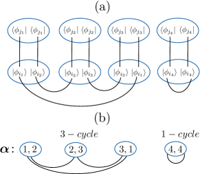
Figure 2: The matching cycles. (a) The ovals represent states of photon pairs. The action of $\hat{P}_{{\boldsymbol{\alpha}}}$ on the ket vectors in $|\mathbf{\Phi}^{(2)}\rangle^{\otimes 4}$ is shown in the bottom ovals (by the curvy lines), whereas the top ovals give the corresponding bra vectors in the inner product $\langle\mathbf{\Phi}^{(2)}|^{\otimes 4}\hat{P}_{{\boldsymbol{\alpha}}}|\mathbf{\Phi}^{(2)}\rangle^{\otimes 4}$. The curvy lines connect the same ket vectors, whereas the vertical lines connect the ket vectors to the respective bra vectors in the inner product. (b)  The cycle decomposition of the corresponding matching ${\boldsymbol{\alpha}}\in\mathcal{M}_{8}$ (in the ovals) acting on the double-set $(1,1,2,2,3,3,4,4)$, composed of the indices of internal modes. There is a $3$-cycle and a $1$-cycle (fixed point).

At this point is it necessary to introduce what will be called the “cycle decomposition” of a matching ${\boldsymbol{\alpha}}\in\mathcal{M}_{2n}$ acting on a double-set $\mathbf{x}\equiv(1,1,\ldots,n,n)$. The double-set appears here due to coinciding indices of the internal states ($|\phi_{j}\rangle$) in each photon pair. Let us rearrange a matching of the double-set, ${\boldsymbol{\alpha}}(\mathbf{x})\equiv(x_{\alpha_{1}},x_{\alpha_{2}},\ldots,x_{\alpha_{2n}})$, as follows. Starting from the first pair $(j_{1},j_{2})$, with $j_{1}=1$ (since $x_{\alpha_{1}}=1$) and $j_{2}=x_{\alpha_{2}}$, we look for the next pair containing $j_{2}$, say $(j_{2},j_{3})$ (permuting the two elements in such a pair, if necessary, to put $j_{2}$ on the first place). We continue by looking for the pair containing now $j_{3}$, etc, until we have come to a pair with $j_{k+1}=j_{1}=1$, for some $1\leq k\leq n$, i.e., we end up with a cycle $\nu$ of length $k$, or $k$-cycle:

$$\nu\equiv\left\{(j_{1},j_{2}),(j_{2},j_{3}),\ldots,(j_{k},j_{1})\right\}.$$ (52)

(Observe that a matching cycle of length $k$ contains $k$ pairs of elements and that each element is repeated.) Then, starting from the smallest $j\notin\nu$ of Eq. (52), quite similarly we end up with another cycle, $\nu^{\prime}$, starting and ending with $j$. We continue until all the elements of $\mathbf{x}$ are arranged in such disjoint cycles (i.e., not having elements in common). In this way, a matching permutation, acting on a double-set, is cast as a product of disjoint cycles.

Denote by $C_{k}({\boldsymbol{\alpha}})$ the total number of $k$-cycles Eq. (52) in a matching ${\boldsymbol{\alpha}}\in\mathcal{M}_{2n}$. The numbers $C_{1},\ldots,C_{n}$ satisfy the obvious constraint $\sum_{k=1}^{n}kC_{k}=n$.

A permutation ${\boldsymbol{\alpha}}$ and the inverse permutation ${\boldsymbol{\alpha}}^{-1}$ correspond to the same cycle structure $(C_{1},\ldots,C_{n})$. Since permutation ${\boldsymbol{\alpha}}$ is cast as the product of disjoint cycles, consider just a single cycle $\nu$, Eq. (52). The cycle $\nu$ of Eq. (52) can be obtained by application of the following cyclic permutation in $S_{n}$ of length $k$

$$j_{k}\to j_{k-1}\to\ldots\to j_{1}\to j_{k}$$ (53)

to the second element in each pair in the trivial matching $\{(j_{1},j_{1}),(j_{2},j_{2}),\ldots,(j_{k},j_{k})\}$. It is easy to see that the inverse permutation $j_{1}\to j_{2}\to\ldots\to j_{k}\to j_{1}$ results in the same cycle $\nu$ (with the pairs permuted; see also appendix C). Hence, $C_{k}({\boldsymbol{\alpha}}^{-1})=C_{k}({\boldsymbol{\alpha}})$ for all $k=1,\ldots,n$.

III.2.2 The output probability

Consider now the matching operator $\hat{P}_{\boldsymbol{\alpha}}$ in Eq. (51). It can be factorized into a product of operators of disjoint cycles $\hat{P}_{\boldsymbol{\alpha}}=\prod_{i}\hat{P}_{\nu_{i}}$. The inner product in Eq. (51) factorizes accordingly. Due to orthogonality of the internal modes, $\langle\phi_{j}|\phi_{j^{\prime}}\rangle=\delta_{jj^{\prime}}$, the operator $\hat{P}_{\nu_{i}}$ of a single cycle has a non-zero contribution to the average in Eq. (51) only when in each inner product of the cycle $\nu_{i}$ the corresponding bra and ket $\phi$-states coincide (i.e., have the same index). As seen from Fig. 2, this necessitates that all the bra and ket $\phi$-states within each independent cycle $\nu_{i}$ coincide (have the same index). Therefore, a $k$-cycle contributes the factor $\sum_{j}p^{k}_{j}$ to $J({\boldsymbol{\alpha}})$, since there are $2k$ products of bra and ket $\phi$-states, each weighed by $\sqrt{p_{j}}$ see Eq. (49). In other words, only the diagonal part of the photon pair state $|\mathbf{\Phi}^{(2)}\rangle\langle\mathbf{\Phi}^{(2)}|$ contributes to output probabilities, where every $k$-cycle contributes a factor equal to the trace of the $k$th power of the diagonal part of the photon pair state.

From the above discussion the distinguishability function $J({\boldsymbol{\alpha}})$ Eq. (51) becomes

$$J({\boldsymbol{\alpha}})=\prod_{k=2}^{n}\Biggl{(}\sum_{j=1}^{\infty}p^{k}_{j}\Biggr{)}^{C_{k}({\boldsymbol{\alpha}})},$$ (54)

where the omitted factor due to $1$-cycles (fixed points) is equal to $1$. The expression in Eq. (54) reminds a similar expression for the distinguishability function of single photons, in the case when each photon is in the same mixed internal state SuffCond ; DTh ; CollPh . In the latter case the cyclic permutations of photons also contribute as independent factors to the distinguishability function. However, there are two new elements here: the cycles rearrange the photon pairs, not single photons, and, therefore, the permutation group $S_{n}$ is replaced by the set of matchings $\mathcal{M}_{2n}$.

With the distinguishability function of Eq. (54) the output probability becomes

$$p_{\mathbf{m}} = \frac{p_{\mathbf{0}}}{\mathbf{m}!}\sum_{{\boldsymbol{\alpha}}\in\mathcal{M}_{2n}}\sum_{{\boldsymbol{\beta}}\in\mathcal{M}_{2n}}\prod_{k=2}^{n}\Biggl{(}\sum_{j=1}^{\infty}p^{k}_{j}\Biggr{)}^{C_{k}({\boldsymbol{\alpha}}^{-1}{\boldsymbol{\beta}})}$$ (55)

$$\times\prod_{i=1}^{n}\mathcal{A}^{*}_{{\alpha_{2i-1}},{\alpha_{2i}}}\mathcal{A}_{{\beta_{2i-1}},{\beta_{2i}}},$$

where $C_{k}({\boldsymbol{\alpha}}^{-1}{\boldsymbol{\beta}})$ is the number of $k$-cycles in the disjoint cycle decomposition of the matching $\mathcal{M}({\boldsymbol{\alpha}}^{-1}{\boldsymbol{\beta}})\in\mathcal{M}_{2n}$. Since $C_{k}({\boldsymbol{\alpha}}^{-1}{\boldsymbol{\beta}})=C_{k}({\boldsymbol{\beta}}^{-1}{\boldsymbol{\alpha}})$, only the real part of the product of matrix elements contributes to the probability in Eq. (55).

A similar expression for the output probability can be derived in the non-degenerate case, when the internal modes for the two polarizations are the same. In this case $|\widetilde{\mathbf{\Phi}}^{(2)}_{k}\rangle=|\mathbf{\Phi}^{(2)}\rangle$ with $|\mathbf{\Phi}^{(2)}\rangle$ of Eq. (49) (recall that the polarizations are excluded from the internal states). Then, by similar arguments as in section III.1 one can show that only the symmetric part of the matrix given by Eq. (45) contributes to the probability and the result is equivalent to that of the degenerate case with the matrix of Eq. (48). Taking this into account, we obtain

$$\tilde{p}_{\mathbf{m}} = \frac{\widetilde{p}_{\mathbf{0}}}{\mathbf{m}!}\sum_{{\boldsymbol{\alpha}}\in{\mathcal{M}}_{2n}}\sum_{{\boldsymbol{\beta}}\in{\mathcal{M}}_{2n}}\prod_{k=2}^{n}\Biggl{(}\sum_{j=1}^{\infty}p^{k}_{j}\Biggr{)}^{C_{k}({\boldsymbol{\alpha}}^{-1}{\boldsymbol{\beta}})}$$ (56)

$$\times\prod_{i=1}^{n}\mathcal{A}^{*}_{\alpha_{2i-1},\alpha_{2i}}\mathcal{A}_{{\beta_{2i-1}},{\beta_{2i}}}$$

where $\mathcal{A}_{ij}\equiv\mathcal{\tilde{A}}^{(s)}_{ij}$ of Eqs. (47)-(48).

III.2.3 Example: Probability to detect four photons

Consider the probability to detect just four photons at interferometer output, i.e. $n=2$. For $n=2$ there are only 1-cycles (i.e., fixed points) and $2$-cycles, thus Eq. (55) depends only on the number of 2-cycles $C_{2}({\boldsymbol{\alpha}}^{-1}{\boldsymbol{\beta}})$. The three permutations in the set $\mathcal{M}_{4}$ are given in Eq. (31). Let us denote $\mu_{2}=(2,3)$ and $\mu_{3}=(2,3,4)$ (respectively, the transposition of $2$ and $3$ and the cycle $2\to 3\to 4\to 2$). Observing that $(2,3)^{-1}=(2,3)$ and $(2,3)(2,3,4)=(2,4)$, we have their action on $\{1,2,3,4\}$:

$$\mu_{2}\left(\begin{array}[]{c}1\\ 2\\ 3\\ 4\end{array}\right)=\left(\begin{array}[]{c}1\\ 3\\ 2\\ 4\end{array}\right),\quad\mu_{3}\left(\begin{array}[]{c}1\\ 2\\ 3\\ 4\end{array}\right)=\left(\begin{array}[]{c}1\\ 4\\ 2\\ 3\end{array}\right)$$ (73)

$$\mu_{2}^{-1}\mu_{3}\left(\begin{array}[]{c}1\\ 2\\ 3\\ 4\end{array}\right)=\mu_{3}^{-1}\mu_{2}\left(\begin{array}[]{c}1\\ 2\\ 3\\ 4\end{array}\right)=\left(\begin{array}[]{c}1\\ 4\\ 3\\ 2\end{array}\right),$$ (86)

$$\mu_{3}^{-1}\left(\begin{array}[]{c}1\\ 2\\ 3\\ 4\end{array}\right)=\left(\begin{array}[]{c}1\\ 3\\ 4\\ 2\end{array}\right).$$ (95)

Now, let us find the number of 2-cycles of the relative permutations acting on the double set $\{1,1,2,2\}$. In this case the index $1\leq i\leq 4$ in Eq. (73) points to the $i$th element in the double set. One can represent the number of 2-cycles for the nine relative permutations ${\boldsymbol{\alpha}}^{-1}{\boldsymbol{\beta}}$, ${\boldsymbol{\alpha}},{\boldsymbol{\beta}}\in\{I,\mu_{2},\mu_{3}\}$ by a matrix $\mathcal{C}_{{\boldsymbol{\alpha}},{\boldsymbol{\beta}}}\equiv C_{2}({\boldsymbol{\alpha}}^{-1}{\boldsymbol{\beta}})$, where

$$\mathcal{C}=\left(\begin{array}[]{ccc}0&1&1\\ 1&0&1\\ 1&1&0\end{array}\right)$$ (96)

with the rows and columns corresponding to ${\boldsymbol{\alpha}}$ and ${\boldsymbol{\beta}}$ in the order $(I,\mu_{2},\mu_{3})$. For instance, $C_{2}(\mu_{3}^{-1}I)=\mathcal{C}_{31}=1$, which can be read from the action of $\mu_{3}^{-1}$ in Eq. (73), projected on the double set as above indicated, and using the definition of a 2-cycle in Eq. (52).

Using Eq. (96) into Eq. (55) we can now write down the probability to detect four photons in an output configuration $\mathbf{m}=(m_{1},\ldots,m_{M})$, $|\mathbf{m}|=4$, where at most four different output ports $1\leq l_{1}\leq l_{2}\leq l_{3}\leq l_{4}\leq M$ are occupied by photons. Recalling that for four photons we have a $4$-dimensional matrix $A_{l_{i}l_{j}}\equiv\mathcal{A}_{ij}=\sum_{k=1}^{N}U_{kl_{i}}r_{k}U_{kl_{j}}$ and using the definition of purity $\mathbb{P}=\sum_{j=1}^{\infty}p^{2}_{j}$ Eq. (3), we obtain

$$p_{\mathbf{m}} = \frac{p_{\mathbf{0}}}{\mathbf{m}!}\Biggl{(}|A_{l_{1}l_{2}}A_{l_{3}l_{4}}|^{2}+|A_{l_{1}l_{3}}A_{l_{2}l_{4}}|^{2}+|A_{l_{1}l_{4}}A_{l_{2}l_{3}}|^{2}$$ (97)

$$+ 2\mathbb{P}\mathrm{Re}\Bigl{\{}\left[A^{*}_{l_{1}l_{3}}A^{*}_{l_{2}l_{4}}+A^{*}_{l_{1}l_{4}}A^{*}_{l_{2}l_{3}}\right]A_{l_{1}l_{2}}A_{l_{3}l_{4}}$$

$$+ A^{*}_{l_{1}l_{3}}A^{*}_{l_{2}l_{4}}A_{l_{1}l_{4}}A_{l_{2}l_{3}}\Bigr{\}}\Biggr{)}.$$

In Eq. (97) the first three terms correspond to $\mathcal{C}_{ii}$ for $i=1,2,3$ and, in the real part, the next two terms to $\mathcal{C}_{1i}$ and $\mathcal{C}_{i1}$, with $i=2,3$, while the last term to $\mathcal{C}_{23}$ and $\mathcal{C}_{32}$.

Let us apply Eq. (97) to the interference on a beamsplitter of two degenerate squeezed states with the squeezing parameters $r_{1}$ and $r_{2}$. We have (without loss of generality)

$$U=\left(\begin{array}[]{cc}u&v\\ -v&u\end{array}\right),\quad u^{2}+v^{2}=1,$$ (98)

where $0\leq u,v\leq 1$. Therefore

$$A=\widetilde{U}\left(\begin{array}[]{cc}r_{1}&0\\ 0&r_{2}\end{array}\right)U=\left(\begin{array}[]{cc}r_{1}u^{2}+r_{2}v^{2}&(r_{1}-r_{2})uv\\ (r_{1}-r_{2})uv&r_{1}v^{2}+r_{2}u^{2}\end{array}\right).$$ (99)

For the five possible output configurations $\mathbf{m}\in\{(4,0),(0,4),(2,2),(3,1),(1,3)\}$ we have the following multisets of output port indices:

$$(4,0)\rightarrow l_{1}=l_{2}=l_{3}=l_{4}=1,$$

$$(0,4)\rightarrow l_{1}=l_{2}=l_{3}=l_{4}=2,$$

$$(2,2)\rightarrow l_{1}=l_{2}=1,\quad l_{3}=l_{4}=2,$$

$$(3,1)\rightarrow l_{1}=l_{2}=l_{3}=1,\quad l_{4}=2,$$

$$(1,3)\rightarrow l_{1}=1,\quad l_{2}=l_{3}=l_{4}=2.$$

Then Eq. (97) gives:

$$p_{(4,0)} = \frac{p_{\mathbf{0}}}{4}A_{11}^{4}\left(\frac{1}{2}+\mathbb{P}\right),\quad p_{(0,4)}=\frac{p_{\mathbf{0}}}{4}A_{22}^{4}\left(\frac{1}{2}+\mathbb{P}\right),$$

$$p_{(2,2)} = \frac{p_{\mathbf{0}}}{4}A^{2}_{11}A^{2}_{22}\left[1+2(1+\mathbb{P})\frac{A_{12}^{4}}{A^{2}_{11}A^{2}_{22}}+4\mathbb{P}\frac{A_{12}^{2}}{A_{11}A_{22}}\right]$$

$$p_{(3,1)} = \frac{p_{\mathbf{0}}}{2}A^{2}_{11}A^{2}_{12}(1+2\mathbb{P}),\;\;p_{(1,3)}=\frac{p_{\mathbf{0}}}{2}A^{2}_{22}A^{2}_{12}(1+2\mathbb{P}).$$

Eq. (LABEL:BSprob) applies also to the interference of a single non-degenerate squeezed state, where now $r_{1}=r_{2}$, hence $A_{11}=A_{22}$, and $A_{12}=0$. This is due to the equivalence of the probability formula between the degenerate and non-degenerate cases, established in section III.1, when the internal modes are the same for the two polarizations in the non-degenerate case. Eq. (LABEL:BSprob) also reproduces the four-photon interference probabilities on the balanced beamsplitter $u=v=1/\sqrt{2}$ in the scheme of Ref. ModeStrInfl . To show this, let us perform post selecting on the detection of four photons at the output, by dividing the results in Eq. (LABEL:BSprob) by the probability to detect exactly four photons

$$p(4)\equiv p_{(4,0)}+p_{(0,4)}+p_{(2,2)}=\frac{p_{\mathbf{0}}}{2}A_{11}^{4}\left(1+\mathbb{P}\right),$$ (101)

(in this case $p_{(1,3)}=p_{(3,1)}=0$). For the non-zero conditional probabilities $P_{\mathbf{m}}\equiv p_{\mathbf{m}}/p(4)$ we get ModeStrInfl

$$P_{(4,0)}=P_{(0,4)}=\frac{1+2\mathbb{P}}{4+4\mathbb{P}},\quad P_{(2,2)}=\frac{1}{2+2\mathbb{P}}.$$ (102)

The above four-photon interference on a beamsplitter of two degenerate squeezed states, or of a single non-degenerate squeezed state in the scheme of Ref. ModeStrInfl , can be used to estimate the purity of the squeezed states. In section IV it will be shown that the effect of distinguishability in the quantum interference with an arbitrary number of squeezed states, each having only two common internal modes, can also be expressed only through the purity.

III.3 Orthogonal internal states

We will use that the output probability, Eq. (III), can be also cast in an equivalent form of a quantum average

$$p_{\mathbf{m}}=\mathrm{Tr}\left\{\hat{\Pi}_{\mathbf{m}}\prod_{k=1}^{N}|r_{k})(r_{k}|\right\}=p_{\mathbf{0}}\binom{2n}{n}\frac{(2n)!}{\mathbf{m}!}$$

$$\times\langle\mathbf{\Psi}^{(2)}|^{\otimes n}\hat{\mathcal{M}}^{\dagger}_{2n}\left[\prod_{i=1}^{2n}|l^{(out)}_{i}\rangle\langle l^{(out)}_{i}|\otimes\openone\right]\hat{\mathcal{M}}_{2n}|\mathbf{\Psi}^{(2)}\rangle^{\otimes n},$$

where we have introduced an unnormalized $2$-particle state

$$|\mathbf{\Psi}^{(2)}\rangle\equiv\sum_{k=1}^{N}\frac{r_{k}}{2}|k\rangle|k\rangle\otimes|\mathbf{\Phi}^{(2)}_{k}\rangle$$ (104)

and observed that $\left[2^{n}(2n-1)!!\right]^{2}=(2n)!\binom{2n}{n}$.

Consider now the case of mutually orthogonal internal states, i.e., $\langle\mathbf{\Phi}^{(2)}_{k^{\prime}}|\mathbf{\Phi}^{(2)}_{k}\rangle=\delta_{k^{\prime}k}$, or, equivalently, $\langle\phi^{(k^{\prime})}_{j^{\prime}}|\phi^{(k)}_{j}\rangle=0$ for $k^{\prime}\neq k$, see Eq. (III). Let us introduce the projectors $\hat{E}_{1},\ldots,\hat{E}_{N}$ onto the internal Hilbert spaces of the squeezed states:

$$\hat{E}_{k}|\phi_{j}^{(k^{\prime})}\rangle=\delta_{k^{\prime}k}|\phi^{(k)}_{j}\rangle,\quad j=1,2,\ldots.$$ (105)

Then, without changing the result, the following substitution can be made in Eq. (III.3)

$$|l^{(out)}_{i}\rangle\langle l^{(out)}_{i}|\otimes\openone\to|l^{(out)}_{i}\rangle\langle l^{(out)}_{i}|\otimes\sum_{k=1}^{N}\hat{E}_{k}.$$ (106)

Moreover, since each squeezed state contributes pairs of photons, only the terms involving pairs of projectors $\hat{E}_{k}$ contribute to the output probability. Thus we can replace the operator in the square brackets in Eq. (III.3) with the one accounting only for all possible occurrences of pairs of $\hat{E}_{k}$:

$$\!\!\!\prod_{i=1}^{2n}\left[|l^{(out)}_{i}\rangle\langle l^{(out)}_{i}|\otimes\sum_{k=1}^{N}\hat{E}_{k}\right]\to\sum_{k_{1}=1}^{N}\ldots\sum_{k_{n}=1}^{N}\frac{1}{(2\mathbf{n})!}$$ (107)

$$\times\sum_{\mu\in S_{2n}}\left[\prod_{i=1}^{2n}|l^{(out)}_{i}\rangle\langle l^{(out)}_{i}|\right]\otimes\left[\prod_{i=1}^{n}\hat{E}_{k_{\mu(i)}}\otimes\hat{E}_{k_{\mu(n+i)}}\right],$$

where the pairs $k_{i}=k_{n+i}$ from $\{1,2,\ldots,N\}$ with the occurrences $\mathbf{n}=(n_{1},\ldots,n_{N})$ are distributed over the output ports by permutation $\mu$ and $(2\mathbf{n})!=(2n_{1})!\ldots(2n_{N})!$ accounts for multiple counting of the same terms. Observe that each term in Eq. (107) describes the detection of photons and the information on the squeezed state each photon came from. For instance, each such term is a collection of configurations $\mathbf{m}^{(k)}=(m^{(k)}_{1},\ldots,m^{(k)}_{M})$, $k=1,\ldots,N$, such that $\mathbf{m}^{(1)}+\ldots+\mathbf{m}^{(N)}=\mathbf{m}$, where the output ports in the configuration $\mathbf{m}^{(k)}$ correspond to the tensor product with the same projector $\hat{E}_{k}$ in the internal subspace. Since the normalization factor is a product as well, $p_{\mathbf{0}}=\mathcal{Z}=\prod_{k=1}^{N}Z_{k}=\prod_{k=1}^{N}{p_{\mathbf{0}}}_{k}$, see Eq. (III), it is now obvious that, due to the mere possibility of complete resolution of the orthogonal internal states of photons at the detection stage, the output probability Eq. (III.3) is a convex mixture of products of the probabilities from the individual squeezed states from different input ports:

$$p_{\mathbf{m}}=\sum p^{(1)}_{\mathbf{m}^{(1)}}\ldots p^{(N)}_{\mathbf{m}^{(N)}},$$ (108)

where the sum is constrained by $\mathbf{m}^{(1)}+\ldots+\mathbf{m}^{(N)}=\mathbf{m}$. In Eq. (108) we have denoted by $p^{(k)}_{\mathbf{m}^{(k)}}$ the probability to detect $2n_{k}=|\mathbf{m}^{(k)}|$ photons from the squeezed state at input port $k$ in the output configuration $\mathbf{m}^{(k)}$, i.e., given by the same formula as in Eq. (55) with the substitutions $p_{\mathbf{0}}\to{p_{\mathbf{0}}}_{k}$ and $\mathcal{A}_{ij}\to\mathcal{A}^{(k)}_{ij}\equiv\mathcal{U}_{ki}r_{k}\mathcal{U}_{kj}$.

III.4 General case of internal states

Consider now the most general case of arbitrary (different) internal modes of photon pairs at different input ports of interferometer. The average of the relative matching operator $\hat{P}^{\dagger}_{{\boldsymbol{\alpha}}}\hat{P}_{{\boldsymbol{\beta}}}$ on the product of the two-photon internal states in Eq. (III) depends on the sets $k_{1},\ldots,k_{n}$ and $k_{1}^{\prime},\ldots,k^{\prime}_{n}$, preventing summation over these indices solely in the product of the matrix elements of $U$. The matching permutations ${\boldsymbol{\alpha}},{\boldsymbol{\beta}}\in\mathcal{M}_{2n}$ Eq. (30) do not form a group (see appendix A), and the relative permutation ${\boldsymbol{\alpha}}^{-1}{\boldsymbol{\beta}}$ may differ from a matching in the standard form of Eq. (30), i.e., ${{\boldsymbol{\alpha}}}^{-1}{{\boldsymbol{\beta}}}\notin\mathcal{M}_{2n}$. Since the tensor product of the internal states to which such a permutation is applied involves generally different states $|\mathbf{\Phi}^{(2)}_{k}\rangle$, one cannot simply project the relative permutation on $\mathcal{M}_{2n}$, as was done in section III.2. In this case one can reverse the substitution of the symmetrization projectors by the matching operators, performed in section III, i.e., replace back

$$\hat{\mathcal{M}}_{2n}\to\hat{S}_{2n}$$ (109)

in Eq. (III). The matchings are then replaced by permutations and the normalization factor is adjusted accordingly. In this way one can get the output probability in the form

$$p_{\mathbf{m}}=\frac{1}{\mathbf{m}!}\frac{p_{\mathbf{0}}}{\left(2^{n}n!\right)^{2}}\sum_{k_{1}=1}^{N}\ldots\sum_{k_{n}=1}^{N}\sum_{k^{\prime}_{1}=1}^{N}\ldots\sum_{k^{\prime}_{n}=1}^{N}\sum_{\sigma\in S_{2n}}\sum_{\tau\in S_{2n}}$$

$$\!\!\!\times\left[\prod_{i=1}^{n}r_{k_{i}}\mathcal{U}^{*}_{k_{i},{\sigma(2i-1)}}\mathcal{U}^{*}_{k_{i},{\sigma(2i)}}r_{k^{\prime}_{i}}\mathcal{U}_{k^{\prime}_{i},{\tau(2i-1)}}\mathcal{U}_{k^{\prime}_{i},{\tau(2i)}}\right]$$

$$\times\langle\mathbf{\Phi}^{(2)}_{k_{1}}|\ldots\langle\mathbf{\Phi}^{(2)}_{k_{n}}|\hat{P}_{\sigma^{-1}\tau}|\mathbf{\Phi}^{(2)}_{k^{\prime}_{1}}\rangle\ldots|\mathbf{\Phi}^{(2)}_{k^{\prime}_{n}}\rangle.$$

In this most general case, the distinguishability function is defined by a complicated expression involving the sets of input indices $k_{1},\ldots,k_{n}$ and $k^{\prime}_{1},\ldots,k^{\prime}_{n}$ as well as permutation $\sigma\in S_{2n}$:

$$J_{\mathbf{k},\mathbf{k}^{\prime}}(\sigma)=\langle\mathbf{\Phi}^{(2)}_{k_{1}}|\ldots\langle\mathbf{\Phi}^{(2)}_{k_{n}}|\hat{P}_{\sigma}|\mathbf{\Phi}^{(2)}_{k^{\prime}_{1}}\rangle\ldots|\mathbf{\Phi}^{(2)}_{k^{\prime}_{n}}\rangle.$$ (111)

There is no other symmetry in Eq. (111) apart from the fact that permutations of the photons within each pair do not change the internal states (in the degenerate case). Thus one can reduce the permutation group $S_{2n}$ in Eq. (111) to the factor group $S_{2n}/S^{\otimes n}_{2}$.

IV Measure of indistinguishability

Let us further analyze the effect of distinguishability in the case of identical internal states $|\mathbf{\Phi}^{(2)}_{k}\rangle=|\mathbf{\Phi}^{(2)}\rangle$ considered in section III.2. Our goal is to quantify the indistinguishability of photons in interference with such squeezed states. We focus on the case of the degenerate squeezed states at interferometer input. The output probability of Eq. (55) can be written also in a similar form as in Eq. (III.3) of section III.3,

$$p_{\mathbf{m}}=\mathrm{Tr}\left\{\hat{\Pi}_{\mathbf{m}}\prod_{k=1}^{N}|r_{k})(r_{k}|\right\}=p_{\mathbf{0}}\binom{2n}{n}\frac{(2n)!}{\mathbf{m}!}$$

$$\times\langle\mathbf{\Psi}^{(2)}|^{\otimes n}\hat{\mathcal{M}}^{\dagger}_{2n}\left[\prod_{i=1}^{2n}|l^{(out)}_{i}\rangle\langle l^{(out)}_{i}|\otimes\openone\right]\hat{\mathcal{M}}_{2n}|\mathbf{\Psi}^{(2)}\rangle^{\otimes n}$$

where

$$|\mathbf{\Psi}^{(2)}\rangle = \left[\sum_{k=1}^{N}\frac{r_{k}}{2}|k\rangle|k\rangle\right]\otimes|\mathbf{\Phi}^{(2)}\rangle$$

$$= \frac{1}{2}\left[\sum_{l=1}^{M}\sum_{s=1}^{M}A_{ls}|l^{(out)}\rangle|s^{(out)}\rangle\right]\otimes|\mathbf{\Phi}^{(2)}\rangle,$$

with $A_{ls}=\sum_{k=1}^{N}U_{kl}r_{k}U_{ks}$.

IV.0.1 A measure of indistinguishability

Let us decompose the internal state $|\mathbf{\Phi}^{(2)}\rangle^{\otimes n}$ of $2n$ photons into the symmetric part and an orthogonal complement, $|\mathbf{\Phi}^{(2)}\rangle^{\otimes n}=\hat{S}_{2n}|\mathbf{\Phi}^{(2)}\rangle^{\otimes n}+(\openone-\hat{S}_{2n})|\mathbf{\Phi}^{(2)}\rangle^{\otimes n}$. We will use the following factorization identity

$$\hat{\mathcal{M}}_{2n}\left(\openone\otimes\hat{S}^{(int)}_{2n}\right)=\hat{\mathcal{M}}^{(op)}_{2n}\otimes\hat{S}^{(int)}_{2n},$$ (114)

where the operator $\hat{\mathcal{M}}_{2n}^{(op)}$ acts on the operational modes only. Eq. (114) can be easily established using the operator composition rule

$$\left(\hat{P}_{\boldsymbol{\alpha}}\otimes\hat{P}_{\boldsymbol{\alpha}}\right)\left(\openone\otimes\hat{P}_{\sigma}\right)=\hat{P}_{\boldsymbol{\alpha}}\otimes\hat{P}_{{\boldsymbol{\alpha}}\sigma}$$

and observing that the permutation $\tau\equiv{\boldsymbol{\alpha}}\sigma$ enumerates all elements of $S_{2n}$. The symmetric part of the internal state $\hat{S}_{2n}|\mathbf{\Phi}^{(2)}\rangle^{\otimes n}$ corresponds to the completely indistinguishable case, since such an internal state factors out, due to the identity in Eq. (114), and does not contribute to the output probability in Eq. (IV).

Let $q_{2n}$ be the probability that the internal state of $2n$ photons is symmetric, i.e.,

$$q_{2n} \equiv \langle\mathbf{\Phi}^{(2)}|^{\otimes n}\hat{S}_{2n}|\mathbf{\Phi}^{(2)}\rangle^{\otimes n}=\langle\mathbf{\Phi}^{(2)}|^{\otimes n}\hat{\mathcal{M}}_{2n}|\mathbf{\Phi}^{(2)}\rangle^{\otimes n}$$ (115)

$$= \frac{1}{(2n-1)!!}\sum_{{\boldsymbol{\alpha}}\in\mathcal{M}_{2n}}J({\boldsymbol{\alpha}}).$$

Though below we discuss the probability $q_{2n}$ only in the case of identical internal states of photon pairs, this probability can be defined in the general case of different internal states

$$q_{2n}=\langle\mathbf{\Phi}^{(2)}_{k_{1}}|\ldots\langle\mathbf{\Phi}^{(2)}_{k_{n}}|\hat{S}_{2n}|\mathbf{\Phi}^{(2)}_{k^{\prime}_{1}}\rangle\ldots|\mathbf{\Phi}^{(2)}_{k^{\prime}_{n}}\rangle,$$ (116)

with the explicit dependence on the input ports of the considered photon pairs (reflected by the indices $k_{j}$ and $k^{\prime}_{j}$).

The introduced probability $q_{2n}$ is the probability that $2n$ photons are indistinguishable, quite similarly as in the case of single photons at interferometer input TBonBS . When $q_{2n}=1$ the identity (114) implies that the photons interfere as completely indistinguishable, i.e., a completely symmetric internal state of $n$ photon pairs has no influence on the output probability distribution. Such a symmetry corresponds to single-mode squeezed states with the same internal mode for all photons.

For identical internals states of photon pairs the probability $q_{2n}$ in Eq. (115) satisfies $q_{2n}\geq\frac{1}{(2n-1)!!}$ thanks to the symmetry of the tensor product of internal states under the permutations of photon pairs and transpositions of two photons in each photon pair. The lower bound is the lowest possible indistinguishability due to the coinciding internal states. It can be shown (see appendix D for details) that the probability $q_{2n}$ in Eq. (115) can be cast as

$$q_{2n} = \sum_{|\mathbf{s}|=n}\binom{n}{\mathbf{s}}\left(\prod_{j=1}^{\infty}p_{j}^{s_{j}}\right)\frac{\prod\limits_{j=1}^{\infty}(2s_{j}-1)!!}{(2n-1)!!}$$

$$= \binom{2n}{n}^{-1}\sum_{|\mathbf{s}|=n}\prod_{j=1}^{\infty}\binom{2s_{j}}{s_{j}}p_{j}^{s_{j}},$$

where $\mathbf{s}=(s_{1},s_{2},\ldots)$, with $s_{j}$ being the number of occurrences of the internal mode $|\phi_{j}\rangle$ in the tensor product of the internal states $|\mathbf{\Phi}^{(2)}\rangle^{\otimes n}$, when the latter is expanded over the tensor products of the internal modes.

The first expression in Eq. (IV.0.1) confirms our interpretation of $q_{2n}$ as the probability of photons behaving as indistinguishable: the multinomial distribution $\binom{n}{\mathbf{s}}\prod_{j}p_{j}^{s_{j}}$ gives the probability of a particular subset of the internal modes $|\phi_{j}\rangle$ of $2n$ interfering photons, whereas the last factor is the probability that in each matching pair the photons have the same internal states (only the indistinguishable photons interfere).

For instance, if there are only two detected photons, they come from the same (degenerate) squeezed state, hence they are indistinguishable. We have $q_{2}=1$. For four detected photons, there are two combinations of non-zero occupations $\mathbf{s}=(s_{1},s_{2},\ldots)$ of photons in the internal modes: $s_{j}=2$ and $s_{j_{1}}=s_{j_{2}}=1$. Hence, we obtain from Eq. (IV.0.1):

$$q_{4} = \binom{4}{2}^{\!-1}\left[\sum_{j=1}^{\infty}\binom{4}{2}p^{2}_{j}+\sum_{j_{1}<j_{2}}\binom{2}{1}^{\!2}p_{j_{1}}p_{j_{2}}\right]$$ (118)

$$= \frac{1+2\mathbb{P}}{3},$$

where we have used the identity $\sum_{j_{1}<j_{2}}p_{j_{1}}p_{j_{2}}=\frac{1}{2}(1-\sum_{j}p^{2}_{j})$ and the definition of the purity Eq. (3). For $n\geq 3$, Eqs. (54) and (115) indicate that that the probability $q_{2n}$ depends also on the higher-order moments of the singular values $\sum_{j}p^{s}_{j}$, $s\leq n$.

The lowest possible indistinguishability $q_{2n}=\frac{1}{(2n-1)!!}$ is attained in Eq. (IV.0.1) for divergent Schmidt number in Eq. (3) $K\to\infty$ (or, equivalently, for vanishing purity $\mathbb{P}\to 0$), i.e., when $p_{j}\to 0$ whereas $\sum_{j}p_{j}=1$. In this limit all higher moments of the singular values, starting from the purity, vanish, $\sum_{j}p^{s}_{j}\to 0$. By using the relation between summations Eq. (19) of section II, we obtain in this case from Eq. (IV.0.1)

$$\lim_{\mathbb{P}\to 0}q_{2n}=\frac{1}{(2n-1)!!}\sum_{j_{1}=1}^{\infty}\ldots\sum_{j_{n}=1}^{\infty}\prod_{i=1}^{n}p_{j_{i}}=\frac{1}{(2n-1)!!},$$ (119)

where we have taken into account that the coincidences $j_{i}=j_{i^{\prime}}$ give a vanishing contribution.

IV.0.2 Bound on the total variation distance

From Eqs. (IV)-(115) we obtain the decomposition of the output probability $p_{\mathbf{m}}$ as follows

$$p_{\mathbf{m}}=q_{2n}\mathring{p}_{\mathbf{m}}+(1-q_{2n})p^{(\perp)}_{\mathbf{m}},$$ (120)

where $\mathring{p}_{\mathbf{m}}$ is given by Eq. (III.1), whereas the complementary probability $p^{\perp}_{\mathbf{m}}$ is obtained by replacing the internal state of $2n$ photons by the complementary part, orthogonal to the symmetric subspace,

$$|\mathbf{\Phi}^{(2)}\rangle^{\otimes n}\to\frac{\openone-\hat{S}_{2n}}{\sqrt{1-q_{2n}}}|\mathbf{\Phi}^{(2)}\rangle^{\otimes n}$$

i.e., the input state of Eq. (IV) is replaced with the following one

$$|\mathbf{\Psi}^{(2n)}_{\perp}\rangle\equiv\openone\otimes\frac{\openone-\hat{S}^{(int)}_{2n}}{\sqrt{1-q_{2n}}}|\mathbf{\Psi}^{(2)}\rangle^{\otimes n},$$ (121)

where $|\mathbf{\Psi}^{(2)}\rangle$ is the state in Eq. (IV). Observe that by construction $p^{(\perp)}_{\mathbf{m}}$ is a normalized probability distribution

$$\sum_{n=0}^{\infty}\sum_{|\mathbf{m}|=2n}p^{(\perp)}_{\mathbf{m}}=1.$$ (122)

Consider now the total variation distance between the output probability distribution $p_{\mathbf{m}}$ of Eq. (120) and that of the ideal case $\mathring{p}_{\mathbf{m}}$ Eq. (III.1). From Eq. (120) we obtain:

$$\mathcal{D} \equiv \frac{1}{2}\sum_{n=0}^{\infty}\sum_{|\mathbf{m}|=2n}|\mathring{p}_{\mathbf{m}}-p_{\mathbf{m}}|$$ (123)

$$= \frac{1}{2}\sum_{n=0}^{\infty}(1-q_{2n})\sum_{|\mathbf{m}|=2n}|\mathring{p}_{\mathbf{m}}-p^{(\perp)}_{\mathbf{m}}|$$

$$\leq \sum_{n=0}^{\infty}(1-q_{2n})\sum_{|\mathbf{m}|=2n}\mathring{p}_{\mathbf{m}}=1-\bar{q}.$$

Here we have used that the variation distance is bounded by the total probability

$$\frac{1}{2}\sum_{|\mathbf{m}|=2n}|\mathring{p}_{\mathbf{m}}-p^{(\perp)}_{\mathbf{m}}|\leq\sum_{|\mathbf{m}|=2n}\mathring{p}_{\mathbf{m}}\equiv\mathring{p}(2n)$$

and introduced the averaged probability $\bar{q}$, where the averaging is over the ideal distribution $\mathring{p}_{\mathbf{m}}$,

$$\bar{q}\equiv\sum_{n=0}^{\infty}\mathring{p}(2n)q_{2n}.$$ (124)

We have (see appendix E)

$$\mathring{p}(2n)=\mathring{p}_{\mathbf{0}}\sum_{|\mathbf{n}|=n}\prod_{k=1}^{N}\binom{2n_{k}}{n_{k}}\left(\frac{r_{k}}{2}\right)^{2n_{k}}$$ (125)

with $\mathring{p}_{\mathbf{0}}=\mathring{\mathcal{Z}}=\prod\limits_{k=1}^{N}\ \left(1-r_{k}^{2}\right)^{\frac{1}{4}}$.

Eqs. (115), (IV.0.1), (120), and (123) allow one to interpret $\bar{q}$ as the measure of average indistinguishability, an analog of a similar measure in the case of interference with single photons at interferometer input TBonBS .

IV.1 Estimate of indistinguishability in the Gaussian boson sampling experiment

We will use that for $N$ equally squeezed single-mode states, $r_{k}=r$ for $k=1,\ldots,N$, the probability to detect $2n$ photons has a simple form, reminiscent of the negative binomial distribution (with a half-integer number of successes $N/2$, in general; see appendix E)

$$\mathring{p}(2n)=(1-r^{2})^{\frac{N}{2}}\left(\frac{N}{2}\right)_{n}\frac{r^{2n}}{n!},$$ (126)

where $(m)_{n}=m(m+1)\ldots(m+n-1)$. With simple algebra one can get the average number of photon pairs and the relative dispersion

$$\bar{n}=\frac{N}{2}\frac{r^{2}}{1-r^{2}},\quad\frac{\overline{n^{2}}-\bar{n}^{2}}{\bar{n}^{2}}=\frac{2}{Nr^{2}}.$$ (127)

Observe that by Eq. (127) for $N\gg 1/r^{2}$ the distribution of the number of detected photons, Eq. (126), becomes sharp about the average, allowing to approximate the average probability of indistinguishable photons $\bar{q}$ Eq. (124) by the most probable value $\bar{q}\approx q_{2\bar{n}}$. The latter can be applied also for the case of almost equal squeezing parameters $r_{k}\approx r$ (recall that $r=\tanh\kappa$, where $\kappa$ is usually called the squeezing parameter).

In the case when the squeezed states are very close to being the single-mode states, one can employ the two-mode approximation consisting of the most probable mode and noise (such a model was used in Ref. ExpGBS2 to characterize purity of the squeezed states). Let the two singular values be $p_{1}=1-\epsilon$ and $p_{2}=\epsilon$, for some $\epsilon\ll 1$. The noise amplitude $\epsilon$ is related to the purity

$$\mathbb{P}\equiv\sum_{j=1,2}p^{2}_{j}=(1-\epsilon)^{2}+\epsilon^{2}.$$ (128)

The two-mode approximation allows to easily evaluate the sum in Eq. (IV.0.1) and estimate the value of $q_{2\bar{n}}$. From the second expression in Eq. (IV.0.1) we obtain

$$\bar{q}\approx q_{2\bar{n}}=\binom{2\bar{n}}{\bar{n}}^{\!-1}\!\!\sum_{s=0}^{\bar{n}}\binom{2s}{s}\binom{2\bar{n}-2s}{\bar{n}-s}\epsilon^{s}(1-\epsilon)^{\bar{n}-s}$$

$$=(1-\epsilon)^{\bar{n}}\mathcal{F}\left(\frac{1}{2},-\bar{n},\frac{1}{2}-\bar{n},\frac{\epsilon}{1-\epsilon}\right)\approx(1-\epsilon)^{\bar{n}},$$ (129)

where $\mathcal{F}$ is the Gauss Hypergeometric function, thus $\mathcal{F}(1/2,-\bar{n},1/2-\bar{n},x)\approx 1$ for $0<x\ll 1$ and arbitrary $\bar{n}$. Eq. (IV.1) predicts that the probability of photons behaving as indistinguishable in an interference with imperfectly single-mode squeezed states falls exponentially fast in the average number of detected photons.

The recent experimental Gaussian boson sampling ExpGBS2 corresponds to $N=50$ degenerate squeezed vacuum states (in an equivalent representation of $N=25$ non-degenerate input states in $N=50$ input ports, see section III) and the squeezing parameters $r_{k}\sim 1$. Let us estimate the indistinguishability in this experiment by employing the average case approximation $\bar{q}\approx q_{2\bar{n}}$ and the above two-mode model of noise. The average reported experimental purity in Ref. ExpGBS2 is $\overline{\mathbb{P}}=0.938$, hence $\epsilon=0.032$ by Eq. (128). The average number of detected photons $2\bar{n}\geq 43$, for the average number of clicks is reported to be 43. Therefore, by Eq. (IV.1) the average probability of photons behaving as completely indistinguishable satisfies $q_{2\bar{n}}\leq 0.5$.

The above discussion leaves out one important question: How can one estimate the indistinguishability parameter $q_{2n}$ from an experiment? Can one estimate the average indistinguishability $q_{2\bar{n}}$ directly from the limited experimental data obtained in experiments on the Gaussian boson sampling? Since limited data allow only to estimate some low-order correlations, is it possible to estimate this parameter from such low-order correlations, e.g., by considering the correlations in a few output ports? The following point should be taken into account: if less than $2\bar{n}$ photons are detected, no higher-order cycles contributing to $q_{2\bar{n}}$ (see Eqs. (54) and (115) and also appendix D) can influence the experimental data. This fact does not allow to directly estimate $q_{2\bar{n}}$ from the low-order correlations, since the latter correspond to much smaller photon numbers as compared to the average total number of detected photons. A similar problem arises also in the case of interference and the boson sampling with single photons, see Refs. SYMDTh ; QPaper . For instance, in Ref. QPaper it was shown that the low-order correlations would be insufficient to distinguish such boson sampling from efficient classical approximations. Similarly here, direct estimate of $q_{2\bar{n}}$ from an experiment requires going beyond the low-order correlations. One way out would be to estimate the purity by the four-photon detection in an interference on a beamsplitter (by using pairs of the degenerate squeezed states or a single non-degenerate squeezed state at a time). From Ref. ModeStrInfl and also from Eq. (LABEL:BSprob) of section III.2 it is seen that the output probability depends on the purity. After that one can get an estimate on the indistinguishability using the above two-mode model.

V Non-Gaussian squeezed states

In the previous sections we have seen the power of the first-order quantization representation for analysis of quantum interference with the Gaussian squeezed states. The purpose of this section is to investigate how the approach can be extended to generalized (non-Gaussian) squeezed vacuum states GenSQ . Such squeezed states are produced by $\mu$-photon processes with $\mu\geq 3$, such as in the recent experimental demonstration of the three-photon spontaneous parametric down-conversion 3phDC . In the parametric approximation, the multi-mode generalized squeezed state can be represented by the following exponential operator

$$|A)\propto\exp\left\{\sum_{i_{1}\in I_{1}}\ldots\sum_{i_{\mu}\in I_{\mu}}A_{i_{1}\ldots i_{\mu}}\hat{c}^{\dagger}_{i_{1}}\ldots\hat{c}^{\dagger}_{i_{\mu}}\right\}|0).$$ (130)

The exponent in Eq. (130) has divergent power series expansion for $\mu>2$ Hillery , as the parametric approximation disregards power depletion in the optical pump SPent ; EnConDC . However, for a finite total number of detected photons one needs to retain only some finite number of terms of the divergent Taylor series. Below the focus will be on the degenerate case corresponding to $I\equiv I_{1}=I_{2}=\ldots=I_{\mu}$ and a symmetric tensor $A$.

For the Gaussian squeezed states, $\mu=2$, the existence of the singular value decomposition of matrices allows one to diagonalize the complex symmetric (generally, infinite-dimensional) matrix $A$ in Eq. (130) to the Schmidt modes MMSS . There is a unitary (also, in general, infinite-dimensional) matrix $V_{ij}$ that

$$A_{il}=\sum_{j\in I}\lambda_{j}V_{ij}V_{lj},$$ (131)

with $\lambda_{j}\geq 0$ being the singular values and columns of $V$ the Schmidt modes $\phi_{j}$. Introducing new boson creation operators by the same unitary transformation

$$\hat{a}^{\dagger}_{j}=\sum_{i\in I}\hat{c}^{\dagger}_{i}V_{ij}$$ (132)

we get the diagonal form of the multi-mode Gaussian squeezed states, which was the starting point in section II, where $\lambda_{j}=r\sqrt{p_{j}}$.

For $\mu\geq 3$ the symmetric tensor $A$ in Eq. (130) can also be similarly diagonalized as a convex sum of the tensor-products of vectors TensorDiag (the columns of the matrix $V$)

$$A_{i_{1}\ldots i_{\mu}}=\sum_{j\in I}\lambda_{j}V_{i_{1}j}\ldots V_{i_{\mu}j}.$$ (133)

However, in this case one has to use, in general, a non-unitary matrix $V_{ij}$. Nevertheless, we can introduce new boson creation operators, similarly to Eq. (132), in order to diagonalize the expression in the exponent in Eq. (130), even if they correspond to some non-orthogonal states. Indeed, the new boson creation operators can be used in the identity Eq. (11), relating the first-order and second-order quantization representations, as the latter remains valid irrespective orthogonality of the single-particle states.

Thus the generalized squeezed states can be reduced in the first-order quantization representation to a simpler diagonal form, similarly as the Gaussian squeezed states. Consider $N$ multi-mode squeezed $\mu$-photon states with the overall squeezing parameters $r_{1},\ldots,r_{N}$ (introduced similarly as in section II, by rescaling $\lambda_{j}=rp_{j}^{1/\mu}$ of the singular values in Eq. (133), where the positive parameters $p_{j}$ sum to $1$). Similarly as in section III, the combined state of $N$ generalized squeezed states can be cast as follows:

$$\prod_{k=1}^{N}|r_{k})\propto\sum_{n=0}^{\infty}\frac{\sqrt{(\mu n)!}}{n!}\hat{S}_{\mu n}\left[\sum_{k=1}^{N}r_{k}\otimes|\mathbf{\Phi}^{(\mu)}_{k}\rangle\right]^{\otimes n},\qquad$$ (134)

$$|\mathbf{\Phi}^{(\mu)}_{k}\rangle\equiv\sum_{j\in I}\left(p^{(k)}_{j}\right)^{\frac{1}{\mu}}|\phi^{(k)}_{j}\rangle^{\otimes\mu}.$$

Now, the state in Eq. (134), to which the projector $\hat{S}_{\mu n}$ is applied, is symmetric with respect to permutations of $\mu$-tuples of photons and with respect to permutations of the photons in each $\mu$-tuple. Let $\mathcal{M}^{(\mu)}_{\mu n}$ be the set of all $\mu$-dimensional matchings, i.e., partitions of $\mu n$ elements $\{1,\ldots,\mu n\}$ into $n$ disjoint $\mu$-tuples $(\alpha_{i\mu+1},\ldots,\alpha_{(i+1)\mu})$, $i=1,\ldots,n$, where permutations of the elements in each $\mu$-tuple do not produce new partitions. The set $\mathcal{M}^{(\mu)}_{\mu n}$ can be enumerated by a vector-index ${\boldsymbol{\alpha}}^{(\mu)}\equiv(\alpha_{1},\ldots,\alpha_{\mu n})$, if we order the $\mu$-dimensional matchings by the first element, where in each $\mu$-tuple we choose as the first element the smallest one by permutation of the elements. It is easy to establish that there are

$$(\mu n-1)!^{(\mu)}\equiv\frac{(\mu n)!}{(\mu!)^{n}n!}$$ (135)

$\mu$-dimensional matchings in $\mathcal{M}^{(\mu)}_{\mu n}$. We can project an arbitrary permutation $\sigma\in S_{\mu n}$ on $\mathcal{M}^{(\mu)}_{\mu n}$ by expanding $\sigma$ as follows

$$\sigma=\pi\left(\tau_{1}\otimes\ldots\otimes\tau_{n}\right){\boldsymbol{\alpha}},$$ (136)

where $\pi\in S_{n}$ permutes $n$ $\mu$-tuples, and $\tau_{i}\in S_{\mu}$ permutes the elements of the $i$th $\mu$-tuple. The symmetrization projector $\hat{S}_{\mu n}$ can be factored accordingly

$$\hat{S}_{\mu n}=\hat{S}^{(tuple)}_{n}\hat{S}_{\mu}^{\otimes n}\hat{\mathcal{M}}^{(\mu)}_{\mu n},$$

$$\hat{\mathcal{M}}^{(\mu)}_{\mu n}\equiv\frac{1}{(\mu n-1)!^{(\mu)}}\sum_{{\boldsymbol{\alpha}}\in\mathcal{M}^{(\mu)}_{\mu n}}\hat{P}_{\boldsymbol{\alpha}}.$$ (137)

Now, due to the symmetry by construction of the state in Eq. (134), the $\mu$-dimensional matching operator $\hat{\mathcal{M}}^{(\mu)}_{\mu n}$ can replace the projector $\hat{S}_{\mu n}$, quite similarly as in the case of the Gaussian squeezed states. One can then proceed from this point.

Summarizing the above, the first-order quantization representation is suitable also or the generalized squeezed states, with, however, a new feature: the equivalent of the Schmidt modes in the diagonal representation are not mutually orthogonal, in general.

VI Conclusion

In conclusion, the first-order quantization representation, commonly underestimated, proves to be extremely useful approach to study the quantum interference of the squeezed vacuum states on a unitary interferometer. It allows for straightforward derivation of the output probability distribution with account the fact that realistic squeezed states possess continuous degrees of freedom, called the Schmidt modes. The method also reproduces previously known results in the limiting cases, e.g., it reproduces the probabilities for the four-photon interference on a beamsplitter and the well-known probability formula for the case of the squeezed states in a single common Schmidt mode.

It is found that the multi-mode structure (i.e., several Schmidt modes) is one of the sources of distinguishability of the squeezed states: each photon pair is effectively in a mixed internal state, which leads to partial distinguishability. A quantitative measure of indistinguishability, $q_{2n}$ is proposed. It is the probability that $n$ pairs of photons interfere as indistinguishable. Moreover, it bounds the total variation distance to the output distribution of the ideal indistinguishable case. In this respect, the proposed measure of indistinguishability is quite similar to that for single photons. It is shown that $q_{2n}$ decreases exponentially fast in $n$. For example, the recent Gaussian boson sampling experiment with the reported purity $\mathbb{P}\approx 0.938$ is, on average, close to the middle line between distinguishable and indistinguishable cases with $q_{2\bar{n}}\lesssim 0.5$ for $2\bar{n}\geq 43$. This fact apparently means that partial distinguishability has also a strong effect on the computational complexity of the output probability distribution from an experimental Gaussian boson sampling. It is known that distinguishability of single photons has a strong effect on the computational complexity of the usual boson sampling.

Finally, the approach of this work is not limited only to the Gaussian states, as it allows for generalization to the generalized (non-Gaussian) squeezed states. Such generalized squeezed states were already observed in the recent three-photon down conversion experiment.

VII acknowledgements

The author is grateful to anonymous referees whose detailed comments helped to improve the presentation. This work was supported by the National Council for Scientific and Technological Development (CNPq) of Brazil, Grant 307813/2019-3.

Appendix A Matchings do not form a group

Counterexamples to the group properties are easily found for $n\geq 3$. Consider the following matching permutation ${\boldsymbol{\alpha}}=(1,5,2,4,3,6)\in\mathcal{M}_{6}$. We have ${\boldsymbol{\alpha}}^{-1}(3)=5>{\boldsymbol{\alpha}}^{-1}(4)=4$, hence ${\boldsymbol{\alpha}}^{-1}\notin\mathcal{M}_{6}$. Additionally, ${\boldsymbol{\alpha}}^{2}=(1,3,5,4,2,6)$ with ${\boldsymbol{\alpha}}^{2}(3)=5>{\boldsymbol{\alpha}}^{2}(4)=4$, hence also ${\boldsymbol{\alpha}}^{2}\notin\mathcal{M}_{6}$. The action of ${\boldsymbol{\alpha}}$ is further illustrated in Eq. (150):

$$\begin{array}[]{cccccc}{\boldsymbol{\alpha}}(1)=\alpha_{1}=1,\\ {\boldsymbol{\alpha}}(2)=\alpha_{2}=5,\\ {\boldsymbol{\alpha}}(3)=\alpha_{3}=2,\\ {\boldsymbol{\alpha}}(4)=\alpha_{4}=4,\\ {\boldsymbol{\alpha}}(5)=\alpha_{5}=3,\\ {\boldsymbol{\alpha}}(6)=\alpha_{6}=6,\end{array}\qquad\begin{array}[]{cccccc}{\boldsymbol{\alpha}}^{2}(1)={\boldsymbol{\alpha}}(\alpha_{1})=1,\\ {\boldsymbol{\alpha}}^{2}(2)={\boldsymbol{\alpha}}(\alpha_{2})=3,\\ {\boldsymbol{\alpha}}^{2}(3)={\boldsymbol{\alpha}}(\alpha_{3})=5,\\ {\boldsymbol{\alpha}}^{2}(4)={\boldsymbol{\alpha}}(\alpha_{4})=4,\\ {\boldsymbol{\alpha}}^{2}(5)={\boldsymbol{\alpha}}(\alpha_{5})=2,\\ {\boldsymbol{\alpha}}^{2}(6)={\boldsymbol{\alpha}}(\alpha_{6})=6.\end{array}$$ (150)

Appendix B Derivation of the output probability

Substituting Eqs. (III), (III) and (38) of the main text in the Born rule and using the identity $(2n)!\binom{2n}{n}\frac{1}{\left[(2n-1)!!\right]^{2}}=2^{2n}$ we obtain

$$p_{\mathbf{m}}=\mathrm{Tr}\left\{\hat{\Pi}_{\mathbf{m}}\prod_{k=1}^{N}|r_{k})(r_{k}|\right\}$$ (151)

$$=\frac{\mathcal{Z}^{2}}{\mathbf{m}!}\sum_{{\boldsymbol{\alpha}},{\boldsymbol{\beta}}}\left[\sum_{k=1}^{N}r_{k}\langle k|\langle k|\otimes\langle\mathbf{\Phi}^{(2)}_{k}|\right]^{\!\otimes n}\hat{P}^{\dagger}_{\boldsymbol{\alpha}}\otimes\hat{P}^{\dagger}_{\boldsymbol{\alpha}}$$

$$\times\left[\prod_{i=1}^{2n}|l^{(out)}_{i}\rangle\langle l^{(out)}_{i}|\otimes\openone\right]\hat{P}_{\boldsymbol{\beta}}\otimes\hat{P}_{\boldsymbol{\beta}}$$

$$\times\left[\sum_{k=1}^{N}r_{k}|k\rangle|k\rangle\otimes|\mathbf{\Phi}^{(2)}_{k}\rangle\right]^{\!\otimes n}.$$

Now we apply the matching operators $\hat{P}_{\boldsymbol{\alpha}}$ and $\hat{P}_{\boldsymbol{\beta}}$ to the output states and expand the tensor products of the linear combinations of two-photon input states. With the use of the input-output relation Eq. (27) we get

$$p_{\mathbf{m}}=\frac{\mathcal{Z}^{2}}{\mathbf{m}!}\sum_{{\boldsymbol{\alpha}},{\boldsymbol{\beta}}}\sum_{k_{1}=1}^{N}\ldots\sum_{k_{N}=1}^{N}\sum_{k^{\prime}_{1}=1}^{N}\ldots\sum_{k^{\prime}_{N}=1}^{N}$$

$$\times\left[\prod_{i=1}^{n}r_{k_{i}}U^{*}_{k_{i}l_{\alpha_{2i-1}}}U^{*}_{k_{i}l_{\alpha_{2i}}}r_{k^{\prime}_{i}}U_{k^{\prime}_{i}l_{\beta_{2i-1}}}U_{k^{\prime}_{i}l_{\beta_{2i}}}\right]$$

$$\times\langle\mathbf{\Phi}^{(2)}_{k_{1}}|\ldots\langle\mathbf{\Phi}^{(2)}_{k_{N}}|\hat{P}^{\dagger}_{{\boldsymbol{\alpha}}}\hat{P}_{{\boldsymbol{\beta}}}|\mathbf{\Phi}^{(2)}_{k^{\prime}_{1}}\rangle\ldots|\mathbf{\Phi}^{(2)}_{k^{\prime}_{N}}\rangle,$$ (152)

which is Eq. (III), taking into account Eq. (39).

Appendix C Cycle index over matchings

Recall that for a permutation group $S_{n}$ acting on the set $\{1,2,\ldots,n\}$, the cycle index Stanley is the sum

$$\Theta_{n} \equiv \sum_{\sigma\in S_{n}}t_{1}^{C_{1}(\sigma)}t_{2}^{C_{2}(\sigma)}\ldots t_{n}^{C_{n}(\sigma)}$$ (153)

$$= \sum_{C_{1},\ldots,C_{n}}\#_{S_{n}}(C_{1},\ldots,C_{n})t_{1}^{C_{1}}t_{2}^{C_{2}}\ldots t_{n}^{C_{n}},$$

$$\#_{S_{n}}(C_{1},\ldots,C_{n})\equiv\frac{n!}{\prod_{k=1}^{n}k^{C_{k}}C_{k}!},$$

where $t_{1},\ldots,t_{n}$ are free parameters, $C_{k}$ is the number of $k$-cycles in the disjoint cycle decomposition of a permutation, the sum over $C_{1},\ldots,C_{n}$ is conditioned on $\sum_{k=1}^{n}kC_{k}=n$, and the factor $\#_{S_{n}}(C_{1},\ldots,C_{n})$ is equal to the total number of permutations $\sigma\in S_{n}$ with a given cycle structure $(C_{1},\ldots,C_{n})$.

Let us now consider a similar cycle index but on the cycles of matching permutations ${\boldsymbol{\alpha}}\in\mathcal{M}_{2n}$ Eq. (30) acting on the double-set $(1,1,2,2,\ldots,n,n)$, i.e.,

$$\Xi_{n} \equiv \sum_{{\boldsymbol{\alpha}}\in\mathcal{M}_{2n}}t_{1}^{C_{1}({\boldsymbol{\alpha}})}t_{2}^{C_{2}({\boldsymbol{\alpha}})}\ldots t_{n}^{C_{n}({\boldsymbol{\alpha}})}$$

$$= \sum_{C_{1},\ldots,C_{n}}\#_{\mathcal{M}_{2n}}(C_{1},\ldots,C_{n})t_{1}^{C_{1}}t_{2}^{C_{2}}\ldots t_{n}^{C_{n}},$$

where the sum over $C_{1},\ldots,C_{n}$ is conditioned on $\sum_{k=1}^{n}kC_{k}=n$, and the cycle decomposition of a matching, when acting on a double-set, is defined in section III.2.

We need to count the number of matchings $\#_{\mathcal{M}_{2n}}(C_{1},\ldots,C_{n})$, from the total number $(2n-1)!!$, which have a given cycle structure $(C_{1},\ldots,C_{n})$. Consider a matching permutation of some given cycle structure, say ${\boldsymbol{\alpha}}\equiv\nu_{1}\nu_{2}\ldots\nu_{q}\in(C_{1},\ldots,C_{n})$, where $\nu_{i}$ are the cycles as defined by Eq. (52) of section III.2. To count the number of matchings for a given cycle structure it is convenient to convert the cycles over the double-set of $2n$ elements $1\leq x_{i}\leq n$ (i.e., with the elements repeated twice) to similar matching cycles over a set of $2n$ distinct elements. This can be done by adding the number $n$ to the second element in each pair, e.g., we make the following transformation of a $k$-cycle defined by Eq. (52)

$$\nu=\{(x_{1},x_{2}),(x_{2},x_{3}),\ldots,(x_{k},x_{1})\}$$ (155)

$$\to\hat{\nu}\equiv\{(x_{1},n+x_{2}),(x_{2},n+x_{3}),\ldots,(x_{k},n+x_{1})\}.$$

Now, for all $k\geq 3$, the transposition of $x_{j}$ with $n+x_{j}$ in a $k$-cycle $\hat{\nu}$ results in a different possible matching ${\boldsymbol{\alpha}}(C_{1},\ldots,C_{n})$ for all $j=1,\ldots,k$, moreover, such transpositions are independent from each other. In the first special case of $k=1$ the only transposition is within a single pair and obviously has no effect. In the second special case of $k=2$, e.g., $\hat{\nu}=\{(x_{1},n+x_{2}),(x_{2},n+x_{1})\}$, only one such transposition (of the two possible) is independent (as we can permute the order of pairs). Summarizing, we get a factor

$$F_{1}\equiv 2^{C_{2}}2^{\sum_{k=3}^{n}kC_{k}}$$ (156)

of how many different matchings in $\mathcal{M}_{2n}$ , i.e., satisfying Eq. (30), there are for a given cycle decomposition of a matching $\{\nu_{1},\ldots,\nu_{q}\}\in(C_{1},\ldots,C_{n})$. What is left is to find out how many cycle decompositions $\{\nu_{1},\ldots,\nu_{q}\}\in(C_{1},\ldots,C_{n})$ there are. To this goal, let us drop in each cycle $\nu_{s}$ the second element in each pair, obtaining on this way a cycle decomposition of a permutation $\sigma\in S_{n}$ (where the sequence of elements, one from each pair, by their order defines a cycle in $S_{n}$). We get a map from the cycles over permutations belonging to $\mathcal{M}_{2n}$, acting on the double-set, to those of the symmetric group $S_{n}$. Note that a $k$-cycle on the double-set has a cyclic order of the pairs: we can choose $x_{j}$ with which a cycle in Eq. (155) will start (recall that, by the definition of such a cycle, we are allowed to permute the two elements inside each pair). On the other hand, the respective $k$-cycle of the symmetric group $S_{n}$ obtained by our map, e.g., from the cycle of Eq. (155) we get $x_{1}\to x_{2}\to\ldots\to x_{k}\to x_{1}$, has a well-defined specific direction, not a cyclic order. We have that for $k\geq 3$ a $k$-cycle and its inverse from $S_{n}$, while being different cycles, nevertheless correspond to one and the same $k$-cycle on the double-set. Thus, we have to account for the double counting of cycles from $\mathcal{M}_{2n}$ by those from $S_{n}$ by introducing the factor

$$F_{2}\equiv\frac{1}{\prod_{k=3}^{n}2^{C_{k}}}$$ (157)

to the number of cycles from $S_{n}$ of a given type $(C_{1},\ldots,C_{n})$, i.e., $\#_{S_{n}}(C_{1},\ldots,C_{n})$ of Eq. (153). Combining the two factors $F_{1}$ and $F_{2}$ given by Eqs. (156)-(157), while using that $\sum_{k=1}^{n}kC_{k}=n$, and applying the result to $\#_{S_{n}}(C_{1},\ldots,C_{n})$ of Eq. (153) we obtain the total number of matchings ${\boldsymbol{\alpha}}\in\mathcal{M}_{2n}$ corresponding to a given cycle structure $(C_{1},\ldots,C_{n})$:

$$\#_{\mathcal{M}_{2n}}(C_{1},\ldots,C_{n})=\#_{S_{n}}(C_{1},\ldots,C_{n})F_{1}F_{2}$$

$$=\frac{2^{n}n!}{\prod_{k=1}^{n}C_{k}!(2k)^{C_{k}}}.$$ (158)

Comparing Eq. (153) with Eqs. (C) and (C), we see that the cycle indices of $\mathcal{M}_{2n}$ and $S_{n}$ are intimately related:

$$\Xi_{n}(t_{1},\ldots,t_{n})=2^{n}\Theta_{n}\left(t_{1}/2,\ldots,t_{n}/2\right).$$ (159)

Appendix D Probability that $n$ pairs of photons are indistinguishable

Using in Eq. (54) of section III.2 the cycle index in Eqs. (153), (C) and (159), by setting $t_{k}=\frac{1}{2}\sum_{j}p^{k}_{j}$ we obtain:

$$q^{(2n)} = \frac{1}{(2n-1)!!}\sum_{{\boldsymbol{\alpha}}\in\mathcal{M}_{2n}}J({\boldsymbol{\alpha}})$$ (160)

$$= \frac{1}{(2n-1)!!}\sum_{C_{1},\ldots,C_{n}}\frac{2^{n}n!}{\prod_{k=1}^{n}C_{k}!(2k)^{C_{k}}}\prod_{k=2}^{n}(2t_{k})^{C_{k}}$$

$$= \frac{2^{n}}{(2n-1)!!}\Theta_{n}\left(t_{1},t_{2},\ldots,t_{n}\right).$$

To compute the cycle index in Eq. (160) we can use the generating function approach Stanley , which reads

$$\Theta_{n}(t_{1},\ldots,t_{n})=\left(\frac{\partial}{\partial x}\right)^{n}\left.\exp\left\{\sum_{k=1}^{\infty}t_{k}\frac{x^{k}}{k}\right\}\right|_{x=0}.$$ (161)

From Eqs. (160)-(161) we get

$$\Theta_{n}(t_{1},\ldots,t_{n})=\left(\frac{\partial}{\partial x}\right)^{n}\left.\exp\left\{\frac{1}{2}\sum_{j=1}^{\infty}\sum_{k=1}^{\infty}\frac{(p_{j}x)^{k}}{k}\right\}\right|_{x=0}$$

$$=\left(\frac{\partial}{\partial x}\right)^{n}\prod_{j=1}^{\infty}(1-p_{j}x)^{-\frac{1}{2}}\Bigr{|}_{x=0}$$

$$=\sum_{|\mathbf{s}|=n}\binom{n}{\mathbf{s}}\prod_{j=1}^{\infty}\left(\frac{\partial}{\partial x}\right)^{n_{j}}(1-p_{j}x)^{-\frac{1}{2}}\Bigr{|}_{x=0}$$

$$=\sum_{|\mathbf{s}|=n}\binom{n}{\mathbf{s}}\prod_{j=1}^{\infty}\frac{1}{2}\left(\frac{1}{2}+1\right)\ldots\left(\frac{1}{2}+s_{j}-1\right)p_{j}^{s_{j}}$$

$$=2^{-n}\sum_{|\mathbf{s}|=n}\binom{n}{\mathbf{s}}\prod_{j=1}^{\infty}(2s_{j}-1)!!p_{j}^{s_{j}},$$ (162)

where we have used the Leibniz rule for derivative, the identity $\ln(1-z)=-\sum\limits_{k=1}^{\infty}\frac{x^{k}}{k}$, denoted by $\mathbf{s}=(s_{1},s_{2},\ldots)$, $|\mathbf{s}|\equiv s_{1}+s_{2}+\ldots=n$, the distribution of $n$ photons over the internal modes $j=1,2,\ldots$ and by $\binom{n}{\mathbf{s}}$ the corresponding multinomial. The probability of Eq. (160) becomes

$$q^{(2n)} = \frac{1}{(2n-1)!!}\sum_{|\mathbf{s}|=n}\binom{n}{\mathbf{s}}\prod_{j=1}^{\infty}(2s_{j}-1)!!p_{j}^{s_{j}}$$ (163)

$$= \binom{2n}{n}^{-1}\sum_{|\mathbf{s}|=n}\prod_{j=1}^{\infty}\binom{2s_{j}}{s_{j}}p_{j}^{s_{j}},$$

where the second form is obtained with the help of the identity

$$\frac{(2m-1)!!}{m!}=2^{-m}\binom{2m}{m}.$$ (164)

Appendix E Probability to detect $2n$ photons

Let us derive the probability $\mathring{p}(2n)$ that exactly $2n$ photons are detected at a multiport output in the ideal case. Consider first the single-mode squeezed state $|r_{k})$ as in Eq. (25) (with $p_{1}=1$). The probability to detect $2n$ photons is given by projection on the Fock state of $2n$ photons and reads

$$\mathring{p}_{k}(2n)=Z^{2}_{k}\binom{2n}{n}\left(\frac{r_{k}}{2}\right)^{2n},$$ (165)

with $Z_{k}=(1-r_{k}^{2})^{\frac{1}{4}}$. Since the probability to detect a given number of photons in all possible output configurations is independent of the interferometer, for a tensor product of $N$ single-mode squeezed states with the squeezing parameters $r_{1},\ldots,r_{N}$, the probability to detect $2n$ photons reads

$$\mathring{p}(2n)=\sum_{|\mathbf{n}|=n}\prod_{k=1}^{N}\mathring{p}_{k}(2n_{k})=\mathring{\mathcal{Z}}^{2}\sum_{|\mathbf{n}|=n}\prod_{k=1}^{N}\binom{2n_{k}}{n_{k}}\left(\frac{r_{k}}{2}\right)^{2n_{k}}$$

with $\mathring{\mathcal{Z}}=\prod_{k=1}^{N}(1-r^{2}_{k})^{\frac{1}{4}}$. The expression can be simplified for the coinciding squeezing parameters $r_{k}=r$. The following identity can be used

$$\sum_{n=0}^{\infty}x^{n}\sum_{|\mathbf{n}|=n}\prod_{k=1}^{N}\binom{2n_{k}}{n_{k}}=\prod_{k=1}^{N}\sum_{n_{k}=0}^{\infty}\binom{2n_{k}}{n_{k}}x^{n_{k}}$$

$$=(1-4x)^{-\frac{N}{2}},$$ (167)

since $\sum_{n=0}^{\infty}\binom{2n}{n}x^{n}=(1-4x)^{-\frac{1}{2}}$. Taking the $n$-th term from the Taylor series of the expression in Eq. (E) we get

$$\sum_{|\mathbf{n}|=n}\prod_{k=1}^{N}\binom{2n_{k}}{n_{k}}=\frac{4^{n}}{n!}\left(\frac{N}{2}\right)_{n},$$ (168)

where $(m)_{n}\equiv m(m+1)\ldots(m+n-1)$. Using Eq. (168) into Eq. (E) for $r_{k}=r$ we obtain

$$\mathring{p}(2n)=(1-r^{2})^{\frac{N}{2}}\left(\frac{N}{2}\right)_{n}\frac{r^{2n}}{n!}.$$ (169)

References

• (1) S. L. Braunstein and P. van Loock, Quantum information with continuous variables, Rev. Mod. Phys. 77, 513 (2005).
• (2) U. L. Andersen, G. Leuchs, and C. Silberhorn, Continuous-variable quantum information processing, Laser Photon. Rev. 4, 337 (2010).
• (3) J.-W. Pan, Z.-B. Chen, C.-Y. Lu, H. Weinfurter, A. Zeilinger, and M. ΕΉukowski, Multiphoton entanglement and interferometry, Rev. Mod. Phys. 84, 777 (2012).
• (4) S. Aaronson and A. Arkhipov, The computational complexity of linear optics, Theory of Computing 9, 143 (2013).
• (5) H. Wang et al, Boson Sampling with 20 Input Photons and a 60-Mode Interferometer in a $10^{14}$-Dimensional Hilbert Space, Phys. Rev. Lett. 123, 250503 (2019).
• (6) D. J. Brod, E. F. GalvΓ£o; A. Crespi, R. Osellame, N. Spagnolo and F. Sciarrino, Photonic implementation of boson sampling: a review, Advanced Photonics, 1, 034001 (2019).
• (7) A. P. Lund, A. Laing, S. Rahimi-Keshari, T. Rudolph, J. L. O’Brien, and T. C. Ralph, Boson Sampling from a Gaussian State, Phys. Rev. Lett. 113, 100502 (2014).
• (8) M. Bentivegna et al, Experimental scattershot boson sampling, Sci. Adv. 1 e1400255 (2015).
• (9) C. S. Hamilton, R. Kruse, L. Sansoni, S. Barkhofen, C. Silberhorn, and I. Jex, Gaussian Boson Sampling, Phys. Rev. Lett. 119, 170501 (2017).
• (10) H.-S. Zhong et al, Experimental Gaussian Boson sampling, Science Bulletin 64, 511 (2019).
• (11) H.-S. Zhong et al, Quantum computational advantage using photons, Science 370, 1460 (2020).
• (12) C. Weedbrook, S. Pirandola, R. GarcΓ­a-PatrΓ³n, N. J. Cerf, T. C. Ralph, J. H. Shapiro, and S. Lloyd, Gaussian quantum information, Rev. Mod. Phys. 84, 621 (2012).
• (13) J. Huh, G. G. Guerreschi, B. Peropadre, J. R. McClean, and A. Aspuru-Guzik, Boson sampling for molecular vibronic spectra, Nat. Photonics 9, 615 (2015).
• (14) L. Banchi, M. Fingerhuth, T. Babej, C. Ing and J. M. Arrazola, Molecular docking with Gaussian Boson Sampling, Science Advances 6, eaax1950 (2020).
• (15) J. M. Arrazola and T. R. Bromley, Using Gaussian Boson Sampling to find dense subgraphs, Phys. Rev. Lett. 121, 030503 (2018).
• (16) K. BrΓ‘dler, P.-L. Dallaire-Demers, P. Rebentrost, D. Su, and C. Weedbrook, Gaussian boson sampling for perfect matchings of arbitrary graphs, Phys. Rev. A, 98, 032310 (2018).
• (17) Z. Vernon, N. Quesada, M. Liscidini, B. Morrison, M. Menotti, K. Tan, and J. E. Sipe, Scalable Squeezed-Light Source for Continuous-Variable Quantum Sampling, Phys. Rev. Applied 12, 064024 (2019).
• (18) C. K. Hong, Z. Y. Ou, and L. Mandel, Measurement of subpicosecond time intervals between two photons by interference, Phys. Rev. Lett. 59, 2044 (1987).
• (19) Z. Y. Ou, Temporal distinguishability of an N-photon state and its characterization by quantum interference, Phys. Rev. A. 74, 063808 (2006).
• (20) S.-H. Tan, Y. Y. Gao, H. de Guise, and B. C. Sanders, SU(3) Quantum Interferometry with Single-Photon Input Pulses, Phys. Rev. Lett. 110, 113603 (2013).
• (21) V. S. Shchesnovich, Sufficient condition for the mode mismatch of single photons for scalability of the boson-sampling computer, Phys. Rev. A 89, 022333 (2014).
• (22) V. S. Shchesnovich, Partial indistinguishability theory for multiphoton experiments in multiport devices, Phys. Rev. A 91, 013844 (2015).
• (23) V. S. Shchesnovich, Tight bound on the trace distance between a realistic device with partially indistinguishable bosons and the ideal BosonSampling, Phys. Rev. A 91, 063842 (2015).
• (24) M. C. Tichy, Sampling of Partially Distinguishable Bosons and the Relation to the Multidimensional Permanent, Phys. Rev. A 91, 022316 (2015).
• (25) M. Tillmann, S.-H. Tan, S. E. Stoeckl, B. C. Sanders, H. de Guise, R. Heilmann, S. Nolte, A. Szameit, and P. Walther, Generalized Multiphoton Quantum Interference, Phys. Rev. X 5, 041015 (2015).
• (26) V. Tamma and S. Laibacher, Multiboson Correlation Interferometry with Arbitrary Single-Photon Pure States, Phys. Rev. Lett. 114, 243601 (2015).
• (27) V. S. Shchesnovich and M. E. O. Bezerra, Collective phases of identical particles interfering on linear multiports, Phys. Rev. A 98, 033805 (2018).
• (28) V. S. Shchesnovich and M. E. O. Bezerra, Distinguishability theory for time-resolved photodetection and boson sampling, Phys. Rev. A 101, 053853 (2020).
• (29) A. E. Moylett and P. S. Turner, Quantum simulation of partially distinguishable boson sampling, Phys. Rev. A 97, 062329 (2018).
• (30) S. Stanisic and P. S. Turner, Discriminating distinguishability, Phys. Rev. A 98, 043839 (2018).
• (31) G. Y. Xiang, Y. F. Huang, F. W. Sun, P. Zhang, Z. Y. Ou, and G. C. Guo, Demonstration of Temporal Distinguishability in a Four-Photon State and a Six-Photon State, Phys. Rev. Lett. 97, 023604 (2006).
• (32) X.-L. Niu, Y.-X. Gong, B.-H. Liu, Y.-F. Huang, G.-C. Guo, and Z. Y. Ou, Observation of a generalized bunching effect of six photons, Opt. lett. 34, 1297 (2009).
• (33) N. Spagnolo, C. Vitelli, L. Sansoni, E. Maiorino, P. Mataloni, F. Sciarrino, D. J. Brod, E. F. GalvΓ£o, A. Crespi, R. Ramponi, and R. Osellame, General Rules for Bosonic Bunching in Multimode Interferometers, Phys. Rev. Lett. 111, 130503 (2013).
• (34) Y.-S. Ra, M. C. Tichy, H.-Tag Lim, O. Kwon, F. Mintert, A. Buchleitner, and Y.-H. Kim, Observation of detection-dependent multi-photon coherence times, Nat. Commun. 4, 2451 (2013).
• (35) A. J. Menssen, A. E. Jones, B. J. Metcalf, M. C. Tichy, S. Barz, W. S. Kolthammer, and I. A. Walmsley, Distinguishability and Many-Particle Interference, Phys. Rev. Lett. 118, 153603 (2017).
• (36) A. E. Jones, A. J. Menssen, H. M. Chrzanowski, T. A. W. Wolterink, V. S. Shchesnovich, and I. A. Walmsley, Multiparticle Interference of Pairwise Distinguishable Photons, Phys. Rev. Lett. 125, 123603 (2020).
• (37) T. BrΓΌnner, G. Dufour, A. RodrΓ­guez, and A. Buchleitner, Signatures of Indistinguishability in Bosonic Many-Body Dynamics, Phys. Rev. Lett. 120, 210401 (2018).
• (38) J. J. Renema, A. Menssen, W. R. Clements, G. Triginer, W. S. Kolthammer, and I. A. Walmsley, Efficient Classical Algorithm for Boson Sampling with Partially Distinguishable Photons, Phys. Rev. Lett. 120, 220502 (2018).
• (39) A. Ferreri, V. Ansari, C. Silberhorn, and P. R. Sharapova, Temporally multimode four-photon Hong-Ou-Mandel interference, Phys. Rev. A 100, 053829 (2019).
• (40) S. L. Braunstein and R. I. McLachlan, Generalized squeezing, Phys. Rev. A 35, 1659 (1987).
• (41) W. S. Chang, C. SabΓ­n, P. Forn-DΓ­az, F. QuijandrΓ­a, A. M. Vadiraj, I. Nsanzineza, G. Johansson, and C. M. Wilson, Observation of Three-Photon Spontaneous Parametric Down-Conversion in a Superconducting Parametric Cavity, Phys. Rev. X 10, 011011 (2020).
• (42) D. Stoler, Equivalence classes of minimum uncertainty packets, Phys. Rev. D 1, 3217 (1970).
• (43) H. P. Yuen, Two-photon coherent states of the radiation field, Phys. Rev. A 13, 2226 (1976).
• (44) R. E. Slusher, P. Grangier, A. LaPorta, B. Yurke, and M. J. Potasek, Pulsed Squeezed Light, Phys. Rev. Lett. 59, 2566 (1987).
• (45) R. Slusher, L. Hollberg, B. Yurke, J. Mertz, and J. Valley, Observation of Squeezed States Generated by Four-Wave Mixing in an Optical Cavity, Phys. Rev. Lett. 55, 2409 (1985).
• (46) Ling-An Wu, H. J. Kimble, J. L. Hall, and Huifa Wu, Generation of Squeezed States by Parametric Down Conversion, Phys. Rev. Lett. 57, 2520 (1986).
• (47) R. M. Shelby, M. D. Levenson, S. H. Perlmutter, R. G. DeVoe, and D. F. Walls, Broad-Band Parametric Deamplification of Quantum Noise in an Optical Fiber, Phys. Rev. Lett. 57, 691 (1986).
• (48) C. Silberhorn, P. K. Lam, O. Weiss, F. KΓΆnig, N. Korolkova, and G. Leuchs, Generation of Continuous Variable Einstein-Podolsky-Rosen Entanglement via the Kerr Nonlinearity in an Optical Fiber, Phys. Rev. Lett. 86, 4267 (2001).
• (49) C. K. Law, I. A. Walmsley, and J. H. Eberly, Continuous Frequency Entanglement: Effective Finite Hilbert Space and Entropy Control, Phys. Rev. Lett. 84, 5304 (2000).
• (50) M. G. Paris, F. Illuminati, A. Serafini, and S. De Siena, Purity of Gaussian states: Measurement schemes and time evolution in noisy channels, Phys. Rev. A 68, 012314 (2003).
• (51) A. Christ, K. Laiho, A. Eckstein, K. N. Cassemiro and C. Silberhorn, Probing multimode squeezing with correlation functions, New J. Phys. 13, 033027 (2011).
• (52) D. B. Horoshko, L. La Volpe, F. Arzani, N. Treps, C. Fabre, and M. I. Kolobov, Bloch-Messiah reduction for twin beams of light, Phys. Rev. A 100, 013837 (2019).
• (53) B. C. Sanders, S. D. Bartlett, T. Rudolph, and P. L. Knight, Photon-number superselection and the entangled coherent-state representation, Phys. Rev. A 68, 042329 (2003).
• (54) T. R. Calixto and P. L. Saldanha, Describing squeezed-light experiments without squeezed-light states, Phys. Rev. A 102, 053723 (2020).
• (55) D. D. Crouch and S. L. Braunstein, Limitations to squeezing in a parametric amplifier due to pump fluctuations, Phys. Rev. A 38, 4696 (1988).
• (56) V. Buzek and G. DrobnΓ½, Signal-pump entanglement in quantum $k$-photon down-conversion, Phys. Rev. A 47, 1237 (1993).
• (57) G. DrobnΓ½ and V. Buzek, Fundamental limit on energy transfer in $k$-photon down-conversion, Phys. Rev. A 50, 3492 (1994).
• (58) V. S. Shchesnovich, The second quantization method for indistinguishable particles, arXiv:1308.3275.
• (59) N. N. Bogolubov and N. N. Bogolubov Jr., Introduction to Quantum Statistical Mechanics (World Scientific Publishing Company; 2nd edition, 2009), see Part II.
• (60) P. A. M. Dirac, The principles of quantum mechanics (Clarendon Press 1966), see chapters IX and X.
• (61) G. J. Milburn, Multimode minimum uncertainty squeezed states, J. Phys. A 17, 737 (1984).
• (62) S. L. Braunstein, Squeezing as an irreducible resource, Phys. Rev. A 71, 055801 (2005).
• (63) E. R. Caianiello, On Quantum Field Theory - I: Explicit Solution of Dyson’s Equation in Electrodynamics without Use of Feynman Graphs, Il Nuovo Cimento 12, 1634 (1953).
• (64) V. S. Shchesnovich, Distinguishing noisy boson sampling from classical simulations, Quantum 5, 423 (2021).
• (65) M. Hillery, Photon number divergence in the quantum theory of n-photon down conversion, Phys. Rev. A 42, 498 (1990).
• (66) P. Comon, G. Golub, L.-H. Lim, and B Mourrain, Symmetric tensors and symmetric tensor rank, SIAM J. Matrix Anal. Appl. 30, 1254 (2008).
• (67) R. P. Stanley, Enumerative Combinatorics, 2nd ed., Vol. 1 (Cambridge University Press, 2011).