Shell-structure and asymmetry effects in level densities

Abstract

Level density $\rho(E,N,Z)$ is derived for a nuclear system with a given energy $E$, neutron $N$, and proton $Z$ particle numbers, within the semiclassical extended Thomas-Fermi and periodic-orbit theory beyond the Fermi-gas saddle-point method. We obtain $~{}~{}\rho\propto I_{\nu}(S)/S^{\nu}$,   where $I_{\nu}(S)$ is the modified Bessel function of the entropy $S$, and $\nu$ is related to the number of integrals of motion, except for the energy $E$. For small shell structure contribution one obtains within the micro-macroscopic approximation (MMA) the value of $\nu=2$ for $\rho(E,N,Z)$. In the opposite case of much larger shell structure contributions one finds a larger value of $\nu=3$. The MMA level density $\rho$ reaches the well-known Fermi gas asymptote for large excitation energies, and the finite micro-canonical limit for low excitation energies. Fitting the MMA $\rho(E,N,Z)$ to experimental data on a long isotope chain for low excitation energies, due mainly to the shell effects, one obtains results for the inverse level density parameter $K$, which differs significantly from that of neutron resonances.

PACS numbers: 21.10.-k, 21.10.Ma, 21.60.Cs, 24.10.Pa

1 Introduction

The statistical level density is a fundamental tool for the description of many properties of heavy nuclei [1, 2, 3, 4, 5, 6, 7, 8, 9, 10, 11, 13, 12, 14, 15, 16, 17, 18, 19, 20, 21, 22, 23]. Usually, the level density $\rho(E,N,Z)$, where $E$, $N$, and $Z$ are the energy, neutron, and proton numbers, respectively, is the inverse Laplace transformation of the partition function $\mathcal{Z}(\beta,\alpha_{n},\alpha_{p})$. Within the grand canonical ensemble, one can apply the standard Darwin-Fowler method for the saddle-point integration over all variables, including $\beta$, which is related to the total energy $E$ [2, 4]. This method assumes large excitation energy $U$, so that the temperature $T$ is related to a well-determined saddle point in the inverse Laplace integration variable $\beta$ for a finite Fermi system of large particle numbers. However, many experimental data also exist for a low-lying part of the excitation energy $U$, where such a saddle point does not exist; see, e.g., Ref. Le20. Therefore, the integral over the Lagrange multiplier $\beta$ in the inverse Laplace transformation of the partition function $\mathcal{Z}(\beta,\alpha_{n},\alpha_{p})$ should be carried out more accurately beyond the standard saddle point method, see Refs. KM79,NPA,PRC. However, for other variables related to the neutron $N$ and proton $Z$ numbers, one can apply the saddle point for large $N$ and $Z$ in a nuclear system. The effects of the pairing correlations in the Fermi system will be worked out separately, see examples in Ref. PRC. Notice that other semi-analytical methods were suggested in the literature [29, 30, 28] to overcome divergence of the full saddle point method for low excitation-energy limit $U\rightarrow 0$.

More general microscopic formulation of the energy level density for mesoscopic systems, in particular for nuclei, which removes the singularity at small excitation energies, is discussed in Ref. ZH19, see also references therein. One of the microscopic ways for accounting for inter-particle interactions beyond the mean field (shell model) in the level density calculations was suggested within the Monte-Carlo Shell Model[31, 11, 13]. Another successful approach for taking into account the inter-particle interactions above the simple shell model is given by the moments method[16, 33, 19, 21, 32]. The main ideas are based on the random matrix theory, see Refs. Po65,Ze96,Ze16,Me04.

For a semiclassical formulation of the unified microscopic canonical and macroscopic grand-canonical approximation (shortly, MMA) to the level density, we will derive a simple non-singular analytical approximation for the level density $\rho$ for neutron-proton asymmetric nuclei. The MMA approach satisfies the two well-known limits. One of them is the Fermi gas asymptote, $\rho\propto\hbox{exp}(S)$, for a large entropy $S$. The opposite limit for small $S$, or excitation energy $U$, is the combinatorics expansion[36, 2, 37] in powers of $S^{2}$. For small excitation energies, the empiric formula, $\rho\propto\hbox{exp}[(U-E_{0})/T]$, with free parameters $E_{0}$, $T$, and a pre-exponent factor was suggested for the description of the level density of the excited low energy states in Ref. GC65. Later, this formula was named as constant “temperature” model, see also Refs. ZK18,ZH19,KZ20. The “temperature” was considered as an “effective temperature” which is related to the excitation energy because of no direct physical meaning of temperature for low energy states. Following the development of Refs. NPA,PRC we will show below that the MMA has the same power expansion as the constant “temperature” model for low energy states at small excitation energies $U$.

Such a MMA for the level density $\rho$ was suggested in Ref. KM79, within the Strutinsky shell correction method[38, 39, 40] based on the Landau-Migdal quasiparticle theory called as the Finite Fermi System Theory[41, 42, 43, 44]. A mean field potential is used for calculations of the energy shell corrections, $\delta E$. The total nuclear energy, $E$, is the sum of these corrections and smooth macroscopic liquid-drop component[45] which can be well approximated by the extended Thomas-Fermi approach [46, 47]. Thus, within the semiclassical approximation to the Strutinsky shell correction method, the interactions between particles, averaged over particle numbers, i.e. over many-body microscopic quantum states in realistic nuclei, are approximately taken into account through the extended Thomas-Fermi component beyond the mean field. Neglecting small residual-interaction corrections (see A) beyond the macroscopic extended Thomas-Fermi approach and Strutinsky’s shell corrections, one can present[25] the level density $\rho$ in terms of the modified Bessel function of the entropy variable in the case of small thermal excitation energy $U$ as compared to the rotational energy.

In order to simplify more the level density calculations for large particle numbers, and for a deeper understanding of the correspondence between the classical and the quantum approach, it is worthwhile to analyze the shell effects in the level density $\rho$ (see Refs. Ig83,So90) and in the entropy, $S$, using the semiclassical periodic-orbit theory [48, 49, 47, 50]. This theory, based on the semiclassical time-dependent propagator, allows obtaining the total level-density, energy, free-energy, and grand canonical potential in terms of the smooth extended Thomas-Fermi term and periodic-orbit correction.

The MMA approach [25] was extended [26, 27] for the description of shell and rotational effects on the level density itself for larger excitation energies $U$ in one-component nucleon systems. We will develop now this MMA for applications to isotopic asymmetric nuclei but for the total level density $\rho(E,N,Z)$, keeping the extension to its spin dependence for a future work. The level density parameter $a$ for asymmetric neutron-proton nuclear system is one of the key quantities under intensive experimental and theoretical investigations[2, 3, 4, 6, 8, 7, 12, 20, 22]. As mean values of $a$ are largely proportional to the total particle number $A$, the inverse level density parameter $K=A/a$ is conveniently introduced to exclude a basic mean $A$-dependence in $a$. Smooth properties of this function of the nucleon number $A$ have been studied within the framework of the self-consistent extended Thomas-Fermi approach[8, 18], see also the study of shell effects in one-component nucleon systems in Refs. NPA,PRC. However, the statistical level density for neutron-proton asymmetric nuclei is still an attractive subject. For instance, within the Strutinsky’s shell correction approach[39], the major shell effects in the distribution of single-particle (quasiparticle) states near the Fermi surface are quite different for neutron and protons of nuclei, especially for nuclei far from the $\beta$-stability line. The present work is concentrated on low energy states of nuclear excitation-energy spectra below the neutron resonances for large chains of the nuclear isotopes.

The structure of the paper is the following. The level density $\rho(E,N,Z)$ is derived within the MMA by using the periodic-orbit theory in Sec. 2. The general shell and isotopic asymmetry effects (Subsections 2.1 and 2.2) are first discussed within the standard saddle-point method asymptote (Subsection 2.3). We then extend the standard saddle-point method to a more general MMA approach for describing the analytical transition from large to small excitation energies $U$, taking essentially into account the shell and isotopic asymmetry effects (Subsection 2.4). In Section 3, we compare our analytical MMA results for the level density $\rho(E,N,Z)$, and the inverse level density parameter $K$ with experimental data for a large isotope chain as typical examples of heavy isotopic asymmetric nuclei. Some details of the Landau-Migdal theory and Strutinsky shell correction method, the periodic-orbit theory, and of the sample method for extraction of the experimental data from nuclear excitation spectra are presented in Appendices A, B and C, respectively.

2 Isotopic asymmetric microscopic-macroscopic approach

2.1 General points

For a statistical description of the level density of a nucleus in terms of the conservation variables; the total energy, $E$; and neutron, $N$, and proton, $Z$, numbers; one can begin with the micro-canonical expression for the level density,

$$\rho(E,N,Z)=\sum\limits_{i}\!\delta(E-E_{i})~{}\delta(N-N_{i})~{}\delta(Z-Z_{i})\equiv\int\frac{\hbox{d}\beta\hbox{d}\alpha_{n}\hbox{d}\alpha_{p}}{(2\pi i)^{3}}~{}e^{S}~{}.$$ (1)

Here, $E_{i}$, $N_{i}$, and $Z_{i}$ represent the system spectrum, and

$$S(\beta,\alpha_{n},\alpha_{p})=\ln\mathcal{Z}(\beta,\alpha_{n},\alpha_{p})+\beta E-\alpha_{n}N-\alpha_{p}Z=\beta(E-\Omega-\lambda_{n}N-\lambda_{p}Z)~{},$$ (2)

where $\alpha_{\tau}=\lambda_{\tau}\beta$, with $\tau=\{n,p\}$ being the isotope subscript. The entropy $S$, partition $\mathcal{Z}$, and potential $\Omega$ functions are considered for arbitrary values of arguments $\beta$ and $\alpha_{\tau}$, and $\Omega=-\ln\mathcal{Z}/\beta$ . The integral on right hand side of Eq. (1) is the standard inverse Laplace transformation of the partition function $\mathcal{Z}$. For large excitation energies, when the saddle points of the integrals (Eq. (1)) over all variables $\beta$, $\alpha_{n}$, and $\alpha_{p}$ exist [6, 7], we have the standard entropy $S$, partition function $\mathcal{Z}$ and thermodynamic potential $\Omega$. In the mean field of the Strutinsky’s shell correction method[39], the single-particle (quasiparticle) level density, $g(\varepsilon)$, can be also written [4] as a sum of the neutron and proton components, $g=g_{n}+g_{p}$ . This leads to a similar isotopic decomposition for the potential $\Omega$, $\Omega=\Omega_{n}+\Omega_{p}$, where $\Omega_{\tau}$ is given by

$$\Omega_{\tau}\approx-\beta^{-1}\int\limits_{0}^{\infty}\hbox{d}\varepsilon~{}g_{\tau}(\varepsilon)~{}\ln\left\{1+\hbox{exp}\left[\beta\left(\lambda_{\tau}-\varepsilon\right)\right]\right\}~{}.$$ (3)

The single-particle level density, $g_{\tau}(\varepsilon)$, within the Strutinsky’s shell-correction method[39], is a sum of the statistically averaged smooth, $\tilde{g}_{\tau}(\varepsilon)$, component, and the oscillating shell, $\delta g_{\tau}(\varepsilon)$, correction, slightly averaged over the single-particle energies,

$$g_{\tau}(\varepsilon)\cong\tilde{g}_{\tau}(\varepsilon)+\delta g_{\tau}(\varepsilon)~{}.$$ (4)

Within the semiclassical periodic-orbit theory[48, 49, 47, 27] (B), the smooth and oscillating parts of the level density, $g_{\tau}(\varepsilon)$, Eq. (4), can be approximated, with good accuracy, by the extended Thomas-Fermi level density, $\tilde{g}_{\tau}\approx g^{(\tau)}_{\rm\tt{ETF}}$, and the periodic-orbit contribution, $\delta g_{\tau}\approx\delta g^{(\tau)}_{\rm scl}$, respectively, see Eq. (37). Using the periodic-orbit theory decomposition, Eq. (4), and Eq. (3), one finds for $\tilde{\Omega}_{\tau}\approx\Omega^{(\tau)}_{\rm\tt{ETF}}$ the result[25, 22]

$$\tilde{\Omega}_{\tau}=\tilde{E}_{\tau}-\lambda_{\tau}A_{\tau}-\frac{\pi^{2}}{6\beta^{2}}\tilde{g}_{\tau}(\lambda_{\tau})~{},\quad A_{\tau}=\{N,Z\}~{}.$$ (5)

Here, $\tilde{E}_{\tau}\approx E^{(\tau)}_{\rm\tt{ETF}}$ is the nuclear extended Thomas-Fermi energy component (or the corresponding liquid-drop energy), and $\lambda_{\tau}\approx\tilde{\lambda}_{\tau}$ is of the smooth chemical potential for neutron ($n$) and proton ($p$) systems in the shell correction method. With the help of the periodic-orbit theory[48, 49, 47, 27], one obtains[25] for the oscillating (shell) component, $\delta\Omega_{\tau}$, Eq. (3),

$$\delta\Omega_{\tau}=-\beta^{-1}\int\limits_{0}^{\infty}\hbox{d}\varepsilon~{}\delta g_{\tau}(\varepsilon)~{}\ln\left\{1+\hbox{exp}\left[\beta\left(\lambda_{\tau}-\varepsilon\right)\right]\right\}\cong\delta\Omega^{(\tau)}_{\rm scl}=\delta F^{(\tau)}_{\rm scl}.$$ (6)

For the semiclassical free-energy shell correction, $\delta F^{(\tau)}_{\rm scl}$, or $\delta\Omega^{(\tau)}_{\rm scl}$, we incorporate the periodic-orbit expression[25, 47]:

$$\delta F^{(\tau)}_{\rm scl}\cong\sum_{\rm PO}F^{(\tau)}_{\rm PO}~{},\quad\mbox{with}\quad F^{(\tau)}_{\rm PO}=E^{(\tau)}_{\rm PO}~{}\frac{x^{(\tau)}_{\rm PO}}{\hbox{sinh}\left(x^{(\tau)}_{\rm PO}\right)}~{},\quad x^{(\tau)}_{\rm PO}=\frac{\pi t^{(\tau)}_{\rm PO}}{\hbar\beta}~{},$$ (7)

where $E^{(\tau)}_{\rm PO}$ is a periodic-orbit component of the semiclassical shell correction energy[48],

$$\delta E^{(\tau)}_{\rm scl}=\sum_{\rm PO}E^{(\tau)}_{\rm PO}~{},\qquad E^{(\tau)}_{\rm PO}=\frac{\hbar^{2}}{(t^{(\tau)}_{\rm PO})^{2}}\,g^{(\tau)}_{\rm PO}(\lambda_{\tau})~{}.$$ (8)

Here, $t^{(\tau)}_{\rm PO}={\tt M}~{}t^{{\tt M}=1}_{\rm PO}(\lambda_{\tau})$ is the period of particle motion along a periodic orbit (taking into account its repetition, or period number ${\tt M}$), and $t^{{\tt M}=1}_{\rm PO}(\lambda_{\tau})$ is the period of the neutron ($n$) or proton ($p$) motion along the primitive (${\tt M}=1$) periodic orbit in the corresponding $\tau$ potential well with the same radius, $R=r_{0}A^{1/3}$. The period $t^{(\tau)}_{\rm PO}$ (and $t^{{\tt M}=1}_{\rm PO}$), and the partial oscillating level density component, $g^{(\tau)}_{\rm PO}$, are taken at the chemical potential, $\varepsilon=\lambda_{\tau}$, see also Eq. (37) for the semiclassical single-particle level-density shell correction (B and Refs. SM76,BB03). The semiclassical expressions, Eqs. (5) and (6), are valid for a large relative action, $\mathcal{S}^{(\tau)}_{\rm PO}/\hbar\sim A^{1/3}\gg 1$ .

Then, expanding $x^{(\tau)}_{\rm PO}/\hbox{sinh}(x^{(\tau)}_{\rm PO})$, Eq. (7), in the shell correction $\delta\Omega_{\tau}$ (Eqs. (6) and (7)) in powers of $1/\beta^{2}$ up to the quadratic terms, $\propto 1/\beta^{2}$, one obtains

$$\Omega_{\tau}\approx E^{(\tau)}_{0}-\lambda_{\tau}A_{\tau}-\frac{a_{\tau}}{\beta^{2}}~{},$$ (9)

where $E^{(\tau)}_{0}$ is the neutron, or proton ground state energy, $E^{(\tau)}_{0}=\tilde{E}_{\tau}+\delta E_{\tau}$, and $\delta E_{\tau}$ is the shell correction energy of the corresponding cold system, $\delta E_{\tau}\approx\delta E^{(\tau)}_{\rm scl}$ (see Eq. (8) and B). In Eq. (9), $a_{\tau}$ is the level density parameter with decomposition similar to Eq. (4):

$$a_{\tau}=\frac{\pi^{2}}{6}~{}g_{\tau}=\tilde{a}_{\tau}+\delta a_{\tau}~{},$$ (10)

where $\tilde{a}_{\tau}$ is the extended Thomas-Fermi component and $\delta a_{\tau}$ is the periodic-orbit shell correction

$$\tilde{a}_{\tau}\approx\frac{\pi^{2}}{6}g^{(\tau)}_{\rm\tt{ETF}}(\lambda_{\tau}),\quad\delta a_{\tau}\approx\frac{\pi^{2}}{6}\delta g^{(\tau)}_{\rm scl}(\lambda_{\tau})~{}.$$ (11)

For the extended Thomas-Fermi component[46, 47, 18, 22], $g^{(\tau)}_{\rm\tt{ETF}}$, one takes into account the self-consistency with Skyrme forces[51]. For the semiclassical periodic-orbit level-density shell corrections[48, 49, 47, 50, 27, 27], $\delta g^{(\tau)}_{\rm scl}(\lambda_{\tau})$, we use Eq. (37).

Expanding the entropy, Eq. (2), over the Lagrange multipliers $\alpha_{\tau}$ near the saddle points $\alpha^{\ast}_{\tau}$, one can use the saddle point equations (particle number conservation equations),

$$\left(\frac{\partial S}{\partial\alpha_{\tau}}\right)^{\ast}\equiv\left(\frac{\partial\ln Z}{\partial\alpha_{\tau}}\right)^{\ast}-A_{\tau}=0~{}.$$ (12)

Integrating then over $\alpha_{\tau}$ in Eq. (1), by the standard saddle-point method, one obtains

$$\rho(E,N,Z)\approx\frac{1}{4\pi^{2}i}\int\hbox{d}\beta~{}\beta\mathcal{J}^{-1/2}\hbox{exp}\left(\beta U+a/\beta\right)~{},$$ (13)

where $U=E-E_{0}$ is the excitation energy ($E_{0}=E^{(n)}_{0}+E^{(p)}_{0}$), and

$$a=a_{n}+a_{p},\qquad g=g_{n}+g_{p}~{},$$ (14)

and $a_{\tau}$ is the $\tau$ component of the level density parameter, given by Eqs. (10), and (11). In equation (13), $\mathcal{J}$ is the two-dimensional Jacobian determinant, $\mathcal{J}(\lambda^{\ast}_{n},\lambda^{\ast}_{p})$, taken at the saddle point, $\lambda_{\tau}=\lambda^{\ast}_{\tau}=\alpha^{\ast}_{\tau}/\beta$, Eq. (12), at a given $\beta$,

$$\mathcal{J}=\mathcal{J}\left(\frac{\partial\Omega}{\partial\lambda_{n}},\frac{\partial\Omega}{\partial\lambda_{p}};\lambda_{n},\lambda_{p}\right)^{\ast}=\left(\frac{\partial^{2}\Omega}{\partial\lambda_{n}^{2}}\frac{\partial^{2}\Omega}{\partial\lambda_{p}^{2}}\right)^{\ast}~{},$$ (15)

where the asterisk indicates the saddle point for the integration over $\alpha_{\tau}$ at any $\beta$. In the following, for simplicity of notations, we will omit the asterisk at $\lambda^{\ast}$.

2.2 Jacobian calculations

Taking the derivatives of Eq. (9) for the potential $\Omega$ with respect to $\lambda_{\tau}$, in the Jacobian $\mathcal{J}$, Eq. (15), up to linear terms in expansion over $1/\beta^{2}$ (Ref. PRC), one obtains

$$\mathcal{J}\approx\mathcal{J}_{0}+\mathcal{J}_{2}/\beta^{2}=\mathcal{J}_{0}\left(1+\xi\right),$$ (16)

where

$$\xi=\overline{\xi}/\beta^{2},\qquad\overline{\xi}=\mathcal{J}_{2}/\mathcal{J}_{0}~{},$$ (17)

with

$$\mathcal{J}_{0}=g_{n}(\lambda_{n})g_{p}(\lambda_{p}),\quad\mathcal{J}_{2}=a^{\prime\prime}_{p}g_{n}(\lambda_{n})+a^{\prime\prime}_{n}g_{p}(\lambda_{p})~{},$$ (18)

see Eqs. (15), and (9). Up to a small asymmetry parameter squared, $~{}~{}X^{2}=$
$(N-Z)^{2}/A^{2}$, one has approximately, $\lambda_{n}=\lambda_{p}=\lambda$, and $~{}g_{n}g_{p}=g^{2}/4~{}$ (see Eq. (14) for $g$). Then, correspondingly, one can simplify Eqs. (18) with (10) to have

$$\mathcal{J}_{0}=\frac{1}{4}g^{2},\quad\mathcal{J}_{2}=\frac{\pi^{2}}{12}g^{\prime\prime}g~{}.$$ (19)

According to Eq. (4), a decomposition of the Jacobian, Eq. (16), in terms of its smooth extended Thomas-Fermi and linear oscillating periodic-orbit components of $\mathcal{J}_{0}$ and $\mathcal{J}_{2}$ can be found straightforwardly with the help of Eqs.(18) and (10) (see also Ref. PRC),

$$\mathcal{J}_{0}=\tilde{\mathcal{J}}_{0}+\delta\mathcal{J}_{0},\qquad\mathcal{J}_{2}=\tilde{\mathcal{J}}_{2}+\delta\mathcal{J}_{2}\approx\delta\mathcal{J}_{2}~{}.$$ (20)

As demonstrated in B, the dominance of derivatives of the semiclassical expression (37) for the single-particle level density shell corrections, $\delta g_{\rm scl}$, in Eq. (19) for $\delta\mathcal{J}_{2}$, led to the last approximation in Eq. (20). For smooth, $\tilde{\mathcal{J}}$, and oscillating, $\delta\mathcal{J}$, components of $\mathcal{J}\cong\tilde{\mathcal{J}}+\delta\mathcal{J}$, Eq. (18), one finds with the help of Eq. (11),

$$\tilde{\mathcal{J}}\approx\tilde{\mathcal{J}}_{0}=\tilde{g}_{n}\tilde{g}_{p}~{},\quad\delta\mathcal{J}=\delta\mathcal{J}_{0}+\delta\mathcal{J}_{2}/\beta^{2},$$ (21)

where $\tilde{g}_{\tau}\approx g^{(\tau)}_{\rm{\tt{ETF}}}(\lambda_{\tau})$ is approximately the (extended) Thomas-Fermi $\tau$-level-density component. For linearized oscillating major-shells components of $\delta\mathcal{J}$, one approximately arrives at

$$\delta\mathcal{J}_{0}\approx\tilde{g}_{n}\delta g_{p}+\tilde{g}_{p}\delta g_{n}~{},\quad\delta\mathcal{J}_{2}\approx-\frac{2\pi^{4}}{3}\left[\frac{\tilde{g}_{n}\delta g_{p}}{\mathcal{D}_{p}^{2}}+\frac{\tilde{g}_{p}\delta g_{n}}{\mathcal{D}_{n}^{2}}\right]~{},$$ (22)

where $\delta g_{\tau}$ is the periodic-orbit shell component, $\delta g_{\tau}\approx\delta g^{(\tau)}_{\rm scl}$ (see Eq. (37)), $\mathcal{D}_{\tau}=\mathcal{D}^{(\tau)}_{\rm sh}=\lambda_{\tau}/A^{1/3}$ is approximately the distance between major (neutron or proton) shells given by Eq. (40). Again, up to terms of the order of $X^{2}$, one simply finds from Eqs. (21) and (22),

$$\tilde{\mathcal{J}}\approx\frac{1}{4}\tilde{g}^{2},\quad\delta\mathcal{J}_{0}\approx\frac{1}{2}\tilde{g}\delta g~{},\quad\delta\mathcal{J}_{2}\approx-\frac{\pi^{4}}{3}\frac{g\delta g}{\mathcal{D}^{2}}~{},$$ (23)

where $\mathcal{D}=\lambda/A^{1/3}$. Note that for thermal excitations smaller or of the order of those of neutron resonances, the main contributions of the oscillating potential, $\delta\Omega_{\tau}$, and Jacobian, $\delta\mathcal{J}$, components as functions of $\lambda_{\tau}$, are coming from the differentiation of the sine in the periodic-orbit level density component, $g^{(\tau)}_{\rm PO}(\lambda_{\tau})$, Eq. (37), through the periodic-orbit action phase $\mathcal{S}^{(\tau)}_{\rm PO}(\lambda_{\tau})/\hbar$. The reason is that, for large particle numbers, $A$, the semiclassically large parameter, $\sim\mathcal{S}^{(\tau)}_{\rm PO}/\hbar\sim A^{1/3}$, leads to dominating contribution, much larger than that coming from differentiation of other terms, such as, the $\beta$-dependent function $x^{(\tau)}_{\rm PO}(\beta)$, and the periodic-orbit period $t^{(\tau)}_{\rm PO}(\lambda)$. Thus, in the linear approximation over $1/\beta^{2}$, we simply arrive to Eq. (22), similarly to the derivations in Ref. PRC.

In the linear approximation in $1/\beta^{2}$, one finds from Eq. (17) for $\xi$ and Eq. (7) for $x^{(\tau)}_{\rm PO}$, see also Eqs. (21), (22) and (14),

$$\overline{\xi}\approx\delta\mathcal{J}_{2}/\tilde{\mathcal{J}_{0}}\approx\overline{\xi}_{n}+\overline{\xi}_{p}~{},\qquad\overline{\xi}_{\tau}=-\frac{2\pi^{4}\delta g_{\tau}}{3\tilde{g}_{\tau}\mathcal{D}^{2}_{\tau}}~{},$$ (24)

see also Eq. (40) for $D_{\tau}$. For convenience, introducing the dimensionless shell correction energy, $\mathcal{E}^{(\tau)}_{\rm sh}$, in units of the smooth extended Thomas-Fermi energy per particle, $E^{(\tau)}_{\rm\tt{ETF}}/A$, one can present Eq. (24) (for $\delta E<0$) as:

$$\overline{\xi}_{\tau}\approx\frac{4\pi^{6}A^{1/3}\mathcal{E}^{(\tau)}_{\rm sh}}{3\lambda^{2}_{\tau}}~{},\quad\mathcal{E}^{(\tau)}_{\rm sh}=-\frac{A\delta E_{\tau}}{E^{(\tau)}_{\rm\tt{ETF}}}~{}.$$ (25)

The smooth extended Thomas-Fermi energy $E^{(\tau)}_{\rm\tt{ETF}}$ can be approximated as $E^{(\tau)}_{\rm\tt{ETF}}\approx\tilde{g}_{\tau}(\lambda_{\tau})\lambda_{\tau}^{2}/2$ . The shell correction energy, $\delta E=\delta E_{n}+\delta E_{p}$, is expressed, for a major shell structure with semiclassical accuracy, through the periodic-orbit sum[48, 49, 47, 50, 27] in Eq. (8), $\delta E_{\tau}\approx\delta E^{(\tau)}_{\rm scl}$, where (see B)

$$\delta E^{(\tau)}_{\rm scl}\approx\left(\frac{D_{\tau}}{2\pi}\right)^{2}~{}\delta g_{\tau}(\lambda_{\tau})~{}.$$ (26)

The correction, $\propto 1/\beta^{4}$, of the expansion in $\propto 1/\beta^{2}$ of both the potential shell correction, Eq. (6) with Eq. (7), and the Jacobian, Eq. (15), through the oscillating part, $\delta\mathcal{J}$, is relatively small for $\beta$ which, evaluated at the critical saddle point values $T=1/\beta^{\ast}$, is related to the chemical potential $\lambda_{\tau}$ as $T\ll\lambda_{\tau}$. Thus, the temperatures $T=1/\beta^{\ast}$, when the saddle point $\beta=\beta^{\ast}$ exists, are assumed to be much smaller than the chemical potentials $\lambda_{\tau}$. The high order, $\propto 1/\beta^{4}$, term of this expansion can be neglected under the following condition (subscripts $\tau$ are omitted for a small asymmetry parameter $(N-Z)^{2}/A^{2}$, see also Ref. PRC):

$$\frac{1}{\tilde{g}}\hbox{\kern 1.00006pt\lower 2.58334pt\hbox{$\sim$} \kern-11.19997pt\raise 2.58334pt\hbox{$<$} \kern 1.00006pt}U\ll\sqrt{\frac{90}{7}}\frac{a\lambda^{2}}{2\pi^{4}A^{2/3}}~{}.$$ (27)

Using typical values for parameters $\lambda\approx 40$ MeV, $A=200$, and $a=A/K\sim 20$ MeV^-1 ($K\sim 10$ MeV), $1/\tilde{g}\sim 0.1-0.2$ MeV, one finds, numerically, that the r.h.s. of this inequality is of the order of the chemical potential, $\lambda$, see Ref. KS18. Therefore, one obtains approximately $U\ll\lambda$. For simplicity, the small shell and temperature corrections to $\lambda_{\tau}(A_{\tau})$ obtained from the conservation equations, Eq. (12), can be neglected. Using the linear shell correction approximation of the leading order [39] and constant particle number density of symmetric nuclear matter, $\rho_{0}=2k_{F}^{3}/3\pi^{2}=0.16$ fm^-3 ($k^{{n}}_{F}\approx k^{{p}}_{F}\approx k_{F}=1.37$ fm^-1 is the Fermi momentum in units of $\hbar$), one finds about a constant value for the chemical potential, $\lambda_{\tau}\approx\hbar^{2}k^{2}_{F}/2m\approx 40$ MeV, where $m$ is the nucleon mass. In the derivations of the condition (27), we used the periodic-orbit theory distances between major shells, $D^{(\tau)}_{\rm sh}$, Eq. (40), $D^{(\tau)}_{\rm sh}\approx\lambda/A^{1/3}$. Evaluation of the upper limit for the excitation energy at the saddle point $\beta=\beta^{\ast}=1/T$ is justified because: this upper limit is always so large that this point does certainly exist. Therefore, for consistency, one can neglect the quadratic, $1/\beta^{2}$ (temperature $T^{2}$), corrections to the Fermi energies $\varepsilon^{(\tau)}_{F}$ in the chemical potential, $\lambda_{\tau}\approx\varepsilon^{(\tau)}_{F}$ (or, $\lambda_{\tau}\approx\lambda\approx\varepsilon_{F}$), for large particle numbers $A$ and small asymmetry parameter $X^{2}$.

2.3 Shell and isotopic asymmetry effects within the saddle-point method

For simplicity, one can start with a direct application of the standard saddle-point approach for calculations of the inverse Laplace integral over $\beta$ in Eq. (13). In this way, including the shell (Ref. PRC) and isotopic asymmetry effects, one arrives at

$$\rho(E,N,Z)\approx\frac{a^{3/4}\hbox{exp}(2\sqrt{aU})}{4\pi~{}U^{5/4}~{}\sqrt{\pi\mathcal{J}_{0}(1+\xi^{\ast})}}\approx\frac{\sqrt{\pi}\hbox{exp}(2\sqrt{aU})}{12a^{1/4}~{}U^{5/4}~{}\sqrt{1+\xi^{\ast}}}~{}.$$ (28)

Here, $a=\pi^{2}g/6$ is the total level density parameter, Eqs. (14) and (11), $\mathcal{J}_{0}$ is the component of the Jacobian $\mathcal{J}$, Eq. (16), which is independent of $\beta$ but depends on the shell structure, and

$$\xi^{\ast}=\frac{\overline{\xi}}{\beta^{\ast\;2}}\approx\frac{2\pi^{4}U}{3aA^{1/3}}\mathcal{E}_{\rm sh}^{\prime\prime}(\lambda)\approx\frac{8\pi^{6}UA^{1/3}}{3a\lambda^{2}}\mathcal{E}_{\rm sh}~{}.$$ (29)

The relative shell correction, $\mathcal{E}_{\rm sh}\approx\mathcal{E}_{\rm sh}^{(\tau)}$, given by Eq. (25), is almost independent of $\tau$ for small $X^{2}$, see also Eqs. (24) and (26). The asterisk means $\beta=\beta^{\ast}=\sqrt{a/U}$ at the saddle point. In the second equation of (28), and of (29) we used $\lambda_{n}\approx\lambda_{p}\approx\lambda$ for a small asymmetry parameter, $X^{2}$, together with Eq. (42) for the derivatives of the energy shell corrections and Eq. (40) for the mean distance between neighboring major shells near the Fermi surface, $\mathcal{D}\approx\lambda/A^{1/3}$.

In Eq. (28), the quantity $\xi^{\ast}$ is $\xi$ in Eq. (17), taken at the saddle point, $\beta=\beta^{\ast}$ ($\lambda_{\tau}=\lambda_{\tau}^{\ast}$). This quantity is the sum of the two $\tau$ contributions, $\xi^{\ast}=\xi^{\ast}_{n}+\xi^{\ast}_{p}$, $~{}~{}\xi^{\ast}_{n}\approx\xi^{\ast}_{p}$. The value of $\xi^{\ast}$ is approximately proportional to the excitation energy, $U$, and to the relative energy shell corrections, $\mathcal{E}_{\rm sh}$, Eq. (25), and inversely proportional to the level density parameter, $~{}a~{}$, with $~{}\xi^{\ast}\propto UA^{1/3}\mathcal{E}_{\rm sh}/(a\lambda^{2})$. For typical parameters $\lambda=40$ MeV, $A\sim 200$, and $\mathcal{E}_{\rm sh}=|\delta E~{}A/E_{\rm\tt{ETF}}|\approx 2.0$ [39, 52], one finds the estimates $\xi^{\ast}\sim 0.1-10$ for temperatures $T\sim 0.1-1$ MeV. This corresponds approximately to a rather wide excitation energies $U=0.2-20$  MeV for $K=A/a=10$ MeV, see Ref. KS18 ($U=0.1-10$ MeV for $K=20$ MeV). This energy range includes the low-energy states and states significantly above the neutron resonances. Within the periodic-orbit theory[48, 47, 50] and extended Thomas-Fermi approach [46, 47, 22], these values are given finally by using the realistic smooth energy $E_{\rm\tt{ETF}}$ for which the binding energy[52] is $BE\approx E_{\rm\tt{ETF}}+\delta E$.

Eq. (28) is a more general shell-structure Fermi-gas (SFG) asymptote, at large excitation energy, with respect to the well-known[1, 2, 3] Fermi gas (FG) approximation for $\rho(E,N,Z)$, which is equal to Eq. (28) at $\xi^{\ast}\rightarrow 0$,

$$\rho(E,N,Z)\rightarrow\frac{\sqrt{\pi}\hbox{exp}(2\sqrt{aU})}{12a^{1/4}~{}U^{5/4}}~{}.$$ (30)

Notice that a shift of the inverse level density parameter $K$ due to shell effects with increasing excitation energies which is related to temperatures of the order of 1-3 MeV is discussed in Refs. PRC,SN90,SN91.

2.4 Shell and isotopic asymmetry effects within the MMA

Under the condition of Eq. (27), one can obtain simple analytical expressions for the level density $\rho(E,N,Z)$, beyond the standard saddle-point method, from the integral representation (13). The square root Jacobian factor $\mathcal{J}^{-1/2}$ in its integrand can be simplified very much by expanding it in small values of $\xi$ or of $1/\xi$ (see Eq. (16)). Expanding now this Jacobian factor at linear order in $\xi$ and $1/\xi$, one arrives at two different approximations marked below by cases (i) and (ii), respectively. Then, taking the inverse Laplace transformation over $\beta$ in Eq. (13), with the transformation of $\beta$ to the inverse variable, $1/\beta$, more accurately (beyond the standard saddle-point[27]), one approximately obtains (see Ref. PRC),

$$\rho\approx\rho_{\tt{MMA}}(S)=\overline{\rho}_{\nu}~{}f_{\nu}(S)~{},~{}~{}~{}f_{\nu}(S)=S^{-\nu}I_{\nu}(S)~{},$$ (31)

with the entropy $S$ given by $S=2\sqrt{aU}$, where $a$ is the sum of the extended Thomas-Fermi term and periodic-orbit shell correction, see Eqs. (14) and (10). For small, $\xi\sim\xi^{\ast}\ll 1$, case (i), and large, $\xi\sim\xi^{\ast}\gg 1$, case (ii), where $\xi^{\ast}$ is, thus, the critical shell-structure quantity, given by expressions (29), $\xi^{\ast}\propto\mathcal{E}_{\rm sh}$, one finds $\nu=2$ for case (i) and $3$ for case (ii), respectively. In case (i) and (ii), called below the MMA1 and MMA2 approaches, respectively, one obtains Eq. (31) with different coefficients $\overline{\rho}_{\nu}$ (see also Ref. PRC),

$$\rho_{\tt{MMA1}}(S)=\overline{\rho}_{2}S^{-2}I_{2}(S),\qquad\overline{\rho}_{2}=\frac{2a^{2}}{\pi\sqrt{\mathcal{J}_{0}}}\approx\frac{2\pi a}{3}\qquad\mbox{(i)},$$ (32)

$$\rho_{\tt{MMA2}}(S)=\overline{\rho}_{3}S^{-3}I_{3}(S),\qquad\overline{\rho}_{3}\approx\frac{4a^{3}}{\pi\sqrt{\overline{\xi}\mathcal{J}_{0}}}\approx\frac{4\pi a^{2}}{3\sqrt{\overline{\xi}}}\qquad\mbox{(ii)},~{}$$ (33)

where $\overline{\xi}$ and $\mathcal{J}_{0}$ are given by Eqs. (17) and (18), respectively, see also Eq. (19) for the last approximations. For the Thomas-Fermi approximation to the coefficient $\overline{\rho}_{3}$ within the case (ii) one finds[26, 27]

$$\rho_{\tt{MMA2b}}(S)=\overline{\rho}^{(2b)}_{3}S^{-3}I_{3}(S),\qquad\overline{\rho}^{(2b)}_{3}\approx\frac{2\sqrt{6}~{}\lambda a^{2}}{3}~{}.$$ (34)

In the derivation of the coefficient, $\overline{\rho}^{(2b)}_{3}$, we assume in Eq. (33) for $\overline{\rho}_{3}$ that the magnitude of the relative shell corrections $\mathcal{E}_{\rm sh}$, $\overline{\xi}\propto\mathcal{E}_{\rm sh}$, see Eqs. (17), (19), and (25), are extremely small but their derivatives yield large contributions through the level density derivatives $g^{\prime\prime}(\lambda)$, $g\propto A/\lambda$, as in the Thomas-Fermi approach. For large entropy $S$, one finds from Eq. (31)

$$f_{\nu}(S)=\frac{\hbox{exp}(S)}{S^{\nu}\sqrt{2\pi S}}\left[1+\frac{1-4\nu^{2}}{8S}+\mbox{O}\left(\frac{1}{S^{2}}\right)\right].$$ (35)

The same leading results in the expansion (35) for $\nu=2$ (i) and $\nu=3$ (ii) at large excitation energies $U$ are also derived from the shell-structure Fermi gas formula (28). At small entropy, $S\ll 1$, one obtains also from Eq. (31) the finite combinatorics power expansion[36, 2, 37]:

$$f_{\nu}(S)=\frac{2^{-\nu}}{\Gamma(\nu+1)}\left[1+\frac{S^{2}}{4(\nu+1)}+\mbox{O}\left(S^{4}\right)\right],$$ (36)

where $\Gamma(x)$ is the Gamma function. This expansion over powers of $S^{2}\propto U$ is the same as that of the constant “temperature” model[3, 19, 20, 21], used often for the level density calculations, but here, as in Ref. PRC, we have it without free fitting parameters.

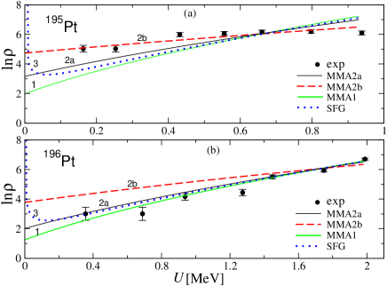
Figure 1: Level density, $\mbox{ln}\rho(E,N,Z)$, for low energy states in nuclei ¹⁹⁵Pt (a), and ¹⁹⁶Pt (b) were calculated within different approximations: The MMA solid green “1” and black “2a”, Eqs.  (32) and (33) at the realistic relative shell correction[52] $\mathcal{E}_{\rm sh}$, respectively; the MMA dashed red “2b”, Eq. (34), and the generalized shell-structure Fermi-Gas rare blue dots, Eq. (28), approaches, respectively, are presented. The realistic values of $\mathcal{E}_{\rm sh}$= 0.77 (a), and 0.84 (b) for MMA2 are taken from Ref. MSIS12 (with chemical potentials $\lambda_{n}\approx\lambda_{p}\approx\lambda$, where $\lambda=40$ MeV). Experimental dots with error bars are obtained from ENSDF database[55] by using the sample method (C).

In contrast to the finite MMA limit (36) for the level density, Eq. (31), the asymptotic SFG (Eq. (28)) and FG (Eq. (30)) expressions are obviously divergent at $U\rightarrow 0$. Notice also that the MMA1 approximation for the level density, $\rho(E,N,Z)$, Eq. (32), can be applied also for large excitation energies, $U$, with respect to the collective rotational excitations, as the SFG and FG approximations if one can neglect shell effects, $\xi^{\ast}\ll 1$. Thus, the level density $\rho(E,N,Z)$ in the case (i), Eq. (32), has wider range of the applicability over the excitation energy variable $U$ than the MMA2 case (ii). The MMA2 approach has, however, another advantage of describing the important shell structure effects. The main effects of the inter-particle interaction, statistically averaged over particle numbers, beyond the shell correction of the mean field within the Strutinsky’s shell correction method was taken into account by the extended Thomas-Fermi components of MMA expression (31) for the level density, $\rho(E,N,Z)$. These components are given by the extended Thomas-Fermi potential, $\Omega_{\rm\tt{ETF}}$, Eq. (5), and the level-density parameter, $a_{\rm\tt{ETF}}$, Eq. (11), counterparts of the corresponding total quantities, Eqs. (3) and (10).

3 Discussion of the results

Fig. 1 and Table 3 show different theoretical (MMA, Eq. (31); SFG, Eq. (28), and; standard FG, Eq. (30)) approaches for the statistical level density $\rho(E,N,Z)$ (in logarithms) as functions of the excitation energy $U$. They are compared to the experimental data obtained by the sample method as explained in C.

The level densities shown in Fig. 1 are calculated using the inverse level density parameter $K$, see Figs. 2 and 3, found from their least mean-square fits to the experimental data for two isotopes of platinum, ¹⁹⁵Pt and ¹⁹⁶Pt, as a typical example. The experimental data shown by dots are obtained for the statistical level density $\rho(E,N,Z)$ from the spectra of nuclear excited states by using the sample method[7] for their distributions (see C).

As in Ref. PRC for isotopes ¹⁶⁶Ho and ¹⁴⁴Sm, Fig. 1 and Table 3 present the two opposite situations concerning the states distributions as functions of the excitation energy $U$. We show results for the nucleus ¹⁹⁵Pt (a) with a large number of the low energy states below excitation energy of about 1 MeV. For ¹⁹⁶Pt (b) one has very small number of low energy states below the same energy of about 1 MeV (see ENSDF database[55] and Table 3 for maximal excitation energies $U_{\rm max}$). But there are many states in ¹⁹⁶Pt with excited energy of above 1 MeV up to essentially larger excitation energy of about 2 MeV. According to Ref. MSIS12, the shell effects, measured by $\mathcal{E}_{\rm sh}$, Eq. (25), are significant in both these deformed nuclei, see Fig. 3(b).

In Fig. 1, the results of the MMA1 and MMA2 approaches, Eqs. (32) and (33), respectively, are compared with the SFG approach, Eq. (28), with a focus on shell effects. The SFG results are very close to those of the well-known FG asymptote, Eq. (30), which neglects the shell effects, see also Table 3. The results of the MMA2a approach, Eq. (33), in the dominating shell effects case (ii) ($\xi^{\ast}\gg 1$, Eq. (29)) with the realistic relative shell correction, $~{}\mathcal{E}_{\rm sh}~{}$ (Ref. MSIS12), are shown versus those of a small shell effects approach MMA1 (i), Eq. (32), valid at $~{}\xi^{\ast}\ll 1~{}$. The results of the limit of the MMA2 to a very small value of $~{}\mathcal{E}_{\rm sh}$,  but still within the case (ii), Eq. (34), called as MMA2b, are also shown in Fig. 1, in contrast to those of the

The inverse level density parameter $K$ (with errors $\Delta K$ in parenthesis) in units of MeV, found by the least mean-square fit for ^175-186Pt in the low energy states ranges restricted by maximal values of the excitation energy having clear spins (from ENSDF database[55]), $U_{\rm max}$ (also in MeV units), with the precision of the standard expression for $\sigma$, Eq. (43), are shown for several approximations with the same notations as in Fig. 1, see also text. The MMA approaches are presented with minimal $\sigma$ which were obtained for the corresponding one-component systems of $A$ nucleons[27]. FG SFG MMA1 MMA2a MMA2b One-component system $U_{\rm max}$ MeV $K$($\Delta K$) MeV $K$($\Delta K$) MeV $K$($\Delta K$) MeV $K$($\Delta K$) MeV $K$($\Delta K$) MeV $K$($\Delta K$) MeV $A$ $\sigma$ $\sigma$ $\sigma$ $\sigma$ $\sigma$ Approach $\sigma$ 175 1.74 13.2 (2.0) 7.2 13.2 (1.9) 7.2 12.0 (2.1) 9.6 19.2 (1.8) 4.9 31.0 (2.0) 2.9 MMA2b 43.5 (2.4) 2.3 176 4.04 26.7 (1.7) 5.6 26.1 (1.6) 5.5 25.2 (1.8) 6.5 27.7 (1.3) 4.8 48.7 (1.4) 2.3 MMA2b 65.6 (1.7) 1.9 177 0.43  3.7 (0.5) 4.3  3.7 (0.5) 4.3  3.4 (0.5) 4.9  6.3 (0.6) 2.9 15.7 (1.1) 1.8 MMA2b 23.1 (1.6) 1.7 178 1.18 12.3 (1.0) 2.1 12.2 (1.0) 2.1 11.2 (1.0) 2.7 15.0 (0.8) 1.6 33.0 (1.2) 0.8 MMA2b 47.2 (1.8) 0.9 179 0.73  5.8 (0.6) 4.9  5.8 (0.6) 4.9  5.3 (0.6) 5.8  8.1 (0.5) 3.2 18.7 (0.7) 1.5 MMA2b 26.8 (1.0) 1.4 180 1.35 13.5 (0.7) 1.8 13.4 (0.7) 1.8 12.5 (0.8) 2.4 15.5 (0.6) 1.5 34.6 (1.1) 1.0 MMA2b 49.2 (1.9) 1.1 181 0.32  3.1 (0.2) 2.2  3.1 (0.2) 2.2  2.9 (0.2) 2.7  5.1 (0.2) 1.5 13.0 (0.8) 1.5 MMA2b 19.0 (1.3) 1.6 182 1.44 14.0 (0.6) 1.6 13.7 (0.5) 1.5 12.9 (0.7) 2.2 15.2 (0.4) 1.3 34.9 (1.4) 1.4 MMA2a 18.5 (0.5) 1.2 183 0.59  4.9 (0.5) 5.8  4.9 (0.5) 5.1  4.5 (0.5) 6.2  6.6 (0.4) 3.5 17.1 (0.6) 1.3 MMA2b 24.7 (0.8) 1.2 184 1.31 13.5 (0.6) 1.4 13.1 (0.6) 1.6 12.5 (0.7) 1.9 14.1 (0.5) 1.4 35.1 (2.1) 1.8 MMA2a 17.1 (0.6) 1.3 185 0.73  5.9 (0.5) 4.4  5.8 (0.4) 4.4  5.5 (0.5) 5.3  7.2 (0.4) 3.3 18.2 (0.5) 1.3 MMA2b 25.7 (1.1) 1.8 186 1.60 15.3 (0.7) 1.9 14.8 (0.6) 1.8 14.2 (0.8) 2.5 15.1 (0.5) 1.8 37.3 (1.3) 1.2 MMA2b 15.1 (0.5) 1.8 187 0.47  3.7 (0.4) 4.7  3.7 (0.4) 4.7  3.4 (0.5) 6.0  5.0 (0.4) 3.4 14.2 (0.7) 1.6 MMA2b 20.6 (1.0) 1.6 188 2.46 19.8 (0.9) 2.8 18.6 (0.7) 2.7 18.6 (1.0) 3.5 18.3 (0.6) 2.8 41.3 (1.2) 1.7 MMA2b 56.7 (2.2) 2.0 189 0.26  2.8 (0.1) 1.3  2.8 (0.1) 1.3  2.5 (0.3) 3.2  4.1 (0.2) 1.3 12.6 (0.3) 0.4 MMA2b 18.6 (0.5) 0.5 190 1.83 15.7 (0.3) 1.8 14.6 (0.3) 1.6 15.1 (0.3) 1.6 14.2 (0.2) 1.8 32.4 (1.7) 4.1 MMA1 18.0 (0.4) 1.8 191 0.56  5.0 (0.7) 6.1 15.8 (0.4) 1.4 15.6 (0.5) 1.7  6.2 (0.6) 4.8 18.0 (1.2) 2.5 MMA2b 30.4 (1.0) 1.7 192 1.79 16.5 (0.9) 2.6 15.5 (0.8) 2.6 15.4 (0.9) 2.8 15.3 (0.7) 2.6 37.6 (2.4) 2.6 MMA1 18.0 (0.4) 1.8 193 0.27  2.9 (0.4) 3.2  2.8 (0.4) 3.2  2.5 (0.5) 4.9  4.0 (0.5) 2.8 15.2 (1.0) 1.3 MMA2b 21.2 (1.5) 1.2 194 1.51 14.3 (0.9) 2.5 13.5 (0.8) 2.5 13.4 (0.8) 2.5 13.4 (0.7) 2.5 33.2 (2.9) 3.1 MMA1 18.0 (0.4) 1.8 195 1.02  7.6 (0.6) 5.8  7.5 (0.6) 5.7  7.1 (0.6) 6.7  8.0 (0.5) 5.0 21.6 (0.7) 2.0 MMA2b 30.4 (1.0) 1.7 196 2.09 15.7 (0.3) 1.8 14.6 (0.3) 1.9 15.1 (0.3) 1.6 14.2 (0.2) 1.8 32.4 (1.7) 4.1 MMA1 18.1 (0.4) 1.8 197 0.77  7.2 (0.9) 5.0  7.1 (0.8) 5.0  6.6 (0.9) 6.0  7.7 (0.7) 4.6 22.9 (1.4) 2.1 MMA2b 32.9 (1.9) 1.9 198 1.37 15.6 (0.9) 1.5 14.5 (0.7) 1.5 14.5 (0.8) 1.7 13.9 (0.6) 1.5 38.4 (2.5) 1.6 MMA2a 16.8 (0.7) 1.5 199 1.24 10.9 (2.3) 7.0 10.4 (2.0) 6.9  9.5 (2.1) 8.6  9.9 (1.6) 7.3 30.4 (3.7) 3.9 MMA2a 43.6 (5.1) 3.5 200 1.84 19.7 (0.8) 1.3 17.6 (0.6) 1.3 18.4 (0.8) 1.6 16.5 (0.6) 1.5 45.3 (2.2) 1.4 MMA2b 63.5 (3.6) 1.6

MMA1 approach. The results of the SFG asymptotical full saddle-point approach, Eq. (28), and of a similar popular FG approximation, Eq. (30), which are both in good agreement with those of the standard Bethe formula[1] for one-component systems (see Ref. PRC), are presented in Table 3. For finite realistic values of $\mathcal{E}_{\rm sh}$, the value of the inverse level density parameter $K$ of MMA2a (Table 3) and the corresponding level density (Fig. 1) are in between those of the MMA1 and MMA2b. Sometimes, the results of the MMA2a approach are significantly closer to those of the MMA1 one, than to those of the MMA2b approach, e.g., for nuclei as ¹⁹⁶Pt.

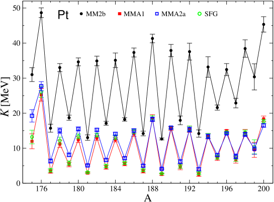
Figure 2: Inverse level density parameters $K$ (with errors) for Pt isotopes are shown as function of the particle numbers $A$ within a long chain A=175-200. Different symbols correspond to several approximations: the close black dots for MMA2b, full red squares for MMA1, larger blue open squares for MMA2a, and green open circles for SFG.

In both panels of Fig. 1, one can see the divergence of the SFG, Eq. (28), level density asymptote in the zero excitation energy limit $U\rightarrow 0$. This is clearly seen also analytically, in particular in the FG limit, Eq. (30); see also the general asymptotic expression (35). It is, obviously, in contrast to any MMAs’ combinatorics expressions (36) in this limit; see Eq. (31). The MMA1 results are close to those of the FG and SFG approaches for all considered nuclei (Table 3), in particular, for both ¹⁹⁵Pt and ¹⁹⁶Pt  isotopes in Table 3. The reason is that their differences are essential only for extremely small excitation energies $U$ where the MMA1 approach is finite while other, FG and SFG, approaches are divergent. However, there are almost no experimental data for excited states in the range of their differences, at least in the nuclei under consideration.

The MMA2b results, Eq. (34), for ¹⁹⁵Pt (see Fig. 1(a)) with $\sigma\sim 1$ are significantly better in agreement with the experimental data as compared to the results of all other approaches (for the same nucleus). For this nucleus, the MMA1 (Eq. (32)), FG (Eq. (30)), and SFG (Eq. (28)) approximations are characterized by much larger $\sigma$ (see Table 3). In contrast to the case of ¹⁹⁵Pt (Fig. 1(a)) with excitation energy spectrum having a large number of low energy states below about 1 MeV, for ¹⁹⁶Pt (Fig. 1(b)) with almost no such states in the same energy range, one finds the opposite case –  a significantly larger MMA2b value of $\sigma$ as compared to those for other approximations (Fig. 2 and Table 3). In particular, for MMA1 (case i), and other asymptotic approaches FG and SFG, one obtains for ¹⁹⁶Pt spectrum almost the same $\sigma\sim 1$, and almost the same for MMA2a (case ii) with realistic values of $\mathcal{E}_{\rm sh}$. Again, notice that the MMA2a results (Eq. (33)) are more close, at the realistic $\mathcal{E}_{\rm sh}$, to those of the MMA1 (case i), as well as the results of the FG and SFG approaches. The MMA1 and MMA2a results (at realistic values of $\mathcal{E}_{\rm sh}$) as well as those of the FG and SFG approaches are obviously much better in agreement with the experimental data[55] (see C) for ¹⁹⁶Pt (Fig. 1(b)).

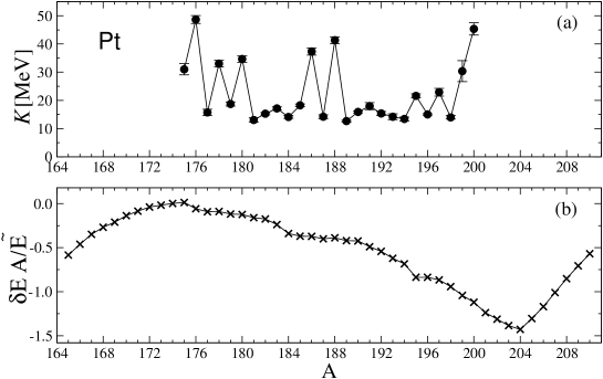
Figure 3: Inverse level density parameters $K$ (with errors) for Pt isotopes are shown as function of the particle numbers $A$ within a long chain A=175-200. (a): the close black dots for the MMA approach taken with the smallest relative error parameter $\sigma$, Eq. (43), among all MMAs. (b): The relative shell correction energies, $\delta EA/\tilde{E}$ are taken from Ref. MSIS12.

One of the reasons of the exclusive properties of ¹⁹⁵Pt (Fig. 1(a)), as compared to ¹⁹⁶Pt (Fig. 1(b)), might be assumed to be the nature of the excitation energy in these nuclei. Our MMAs results (case i) or (case ii) could clarify the excitation nature as assumed in Ref. PRC. Since the MMA2b results (case ii) are much better in agreement with the experimental data than the MMA1 results (case i) for ¹⁹⁵Pt, one could presumably conclude that for ¹⁹⁵Pt one finds more clear thermal low-energy excitations. In contrast to this, for ¹⁹⁶Pt (Fig. 1(b)), one observes more regular high-energy excitations coming, e.g., from the dominating rotational energy $E_{\rm rot}$, see Refs. KM79,PRC. As seen, in particular, from the values of the inverse level density parameter $K$ and the shell structure of the critical quantity, $\xi^{\ast}\propto\mathcal{E}^{\prime\prime}_{\rm sh}/a=K\mathcal{E}^{\prime\prime}_{\rm sh}/A$, Eq. (29), these properties can be understood to be mainly due to the larger values of $K$ and shell correction second derivative $\mathcal{E}^{\prime\prime}_{\rm sh}$, for low energy states in ¹⁹⁵Pt (Table 3) versus those of the ¹⁹⁶Pt spectrum. This is in addition to the shell effects, which are very important for the case (ii) which is not even realized without their dominance.

As results, the statistically averaged level densities $\rho(E,N,Z)$ for the MMA with a minimal value of the control-error parameter $\sigma$, Eq. (43), in plots of Fig. 1 agree well with those of the experimental data. The results of the MMA, SFG and FG approaches for the level densities $\rho(E,N,Z)$ in Fig. 1, and for $K$ in Table 3, do not depend on the cut-off spin factor and moment of inertia because of the summations (integrations) over all spins, indeed, with accounting for the degeneracy $2I+1$ factor. We do not use empiric free fitting parameters in our calculations, in particular, for the FG results shown in Table 3, in contrast to the back-shifted Fermi gas[56] and constant temperature models, see also Ref. EB09.

The results of calculations for the inverse level density parameter $K$ in the long Pt isotope chain with $A=175-200$ are summarized in Fig. 2 and Table 3. Preliminary spectra data for nuclei far away from the $\beta$-stability line from Ref. ENSDFdatabase are included in comparison with the results of the theoretical approximations. These experimental data, may be incomplete. Nevertheless, it might be helpful to present the comparison between theory and experiment to check general common effects of the statistical isotopic asymmetry and shell structure in a more wide range of nuclei around the $\beta$-stability line.

As seen in Fig. 2, the results for $K$ for the isotopes of Pt ($Z=78$) as a function of the particle number $A$ are characterized by a very pronounced saw-toothed behavior with the alternating low and high $K$ values for odd and even nuclei, respectively. This behavior is more pronounced for the MMA2b (close black dots) with larger $K$ values. For each nucleus, the significantly smaller MMA1 value of $K$ (full red squares) is close to that of the SFG (open green circles). The FG results are very close to those of the SFG approach and, therefore, are not shown in the plots, but presented in the Table. The MMA2a results for $K$ are intermediate between the MMA2b and MMA1 ones, but closer to the MMA1 values.

Notice that for rather a long chain of the isotopes of Pt, one finds the remarkable shell oscillation (Fig. 2). Fixing the even-even (even-odd) chain, for all compared approximations, one can see a hint of slow oscillations by evaluating its period $\Delta A$, $\Delta A\sim 40$ for $A\sim 200$ (see Ref. NPA and Eq. (41)). Within order of magnitude, these estimates agree, with the main period for the relative shell corrections, $\delta EA/\tilde{E}$, shown in Fig. 3(b). Therefore, according to these evaluations and Fig. 3(b) for $K(A)$, we show the sub-shell effects within a major shell. This shell oscillation as function of $A$ is more pronounced for the MMA2b case because of its relatively large amplitude, but is mainly proportional to that of the MMA2a and other approximations.

The MMAs results shown in Fig. 2, as function of the particle number $A$, Eq. (29), can be partially understood through the basic critical quantity, $\xi\sim\xi^{\ast}\leq\xi^{\ast}_{\rm max}$, where $\xi^{\ast}_{\rm max}\propto KU_{\rm max}\mathcal{E}^{\prime\prime}_{\rm sh}/A^{4/3}$ . Here we need also the maximal excitation energies $U_{\rm max}$ of the low energy states (from Ref. ENSDFdatabase and Table 3) used in our calculations. Such low energy states spectra are more complete due to information on the spins of the states. We extended the particle number interval beyond the range of known spectra in Fig. 3(b) to demonstrate a clear major shell. As assumed in the derivations (Subsection 2.4), larger values of $\xi^{\ast}$, Eq. (29), are expected in the MMA2b approximation (see Fig. 2), first of all because of large $K$ (small level density parameter $a$). For the MMA1 approach, one finds significantly smaller $\xi^{\ast}$, and in between values (more close to the MMA1) for the MMA2a case. This is in line with the assumptions for case (i) and case (ii) in the derivations of the MMA1, Eq. (32), and MMA2, Eq. (33), level-density approximations, respectively.

In order to clarify the shell effects, we present in Fig. 3(a) the inverse level density parameters $K(A)$ taking the MMA results with the smallest values of $\sigma$ at each nucleus (see Fig. 2 and Table 3). Among all MMAs results, this provides the best agreement with the experimental data for the statistical level density obtained by the sample method (C). The relative energy shell corrections[52], $\delta EA/\tilde{E}\approx\delta EA/BE$, are presented by crosses in Figure 3(b).

The oscillations in Fig. 3(a) are associated with sub-shell effects within the major shell, shown in Fig. 3(b). As seen from Fig. 3 and Table 3, the results of the MMA2b approach the better agree with experimental data the larger number of states in the low energy states range and the smaller maximal excitation energies, $U_{\rm max}$. This is not the case for the MMA1 and other approaches. One of the most pronounced cases was considered above for the ¹⁹⁵Pt and ¹⁹⁶Pt nuclei. However, in the middle of the Pt chain, the results of all approximations are not well distinguished because of almost the same $\sigma$. Except for the nuclei ^176,188Pt, where one has relatively large $U_{\rm max}$, for significantly smaller $U_{\rm max}$ the MMA2b approach is obviously better than other approaches. Most of the Pt isotopes under the consideration are well deformed, and the excited energy spectra (Ref. ENSDFdatabase) begin with relatively small energy levels in the low energy states region. Therefore, for simplicity, the pairing effects were not taken into account in our Pt calculations, even in the simplest version[27] of a shift of the excitation energy by pairing condensation energy. We should emphasize once more that the MMA2 approach for each of nucleus is important in the case (ii) of dominating shell effects (see Subsection 2.4). As shown in the Table, the isotopic asymmetry effects are important as compared to those of the corresponding one-component nucleon case[27]. They decrease significantly the inverse level density parameter $K$, especially for the MMA2b approach.

Thus, for the Pt isotope chain, one can clearly see almost major shell region and approximately constant mean values of $K(A)$ for each approximation (Fig. 2). The MMA1 approach yields essentially small values for $K$, which are closer to that of the neutron resonances. Their values are a little smaller than those of the MMA2a, and much smaller than those of the MMA2b approach (Fig. 2). As seen clearly from Figs. 2 and 3, and Table 3, in line with results of Ref. ZS16, the obtained values for $K$ within the MMA2 approach can be essentially different from those of the MMA1 approach and those of the SFG and FG approaches found, mainly, for the neutron resonances. Notice that, as in Ref. NPA, in all our calculations of the statistical level density, $\rho(E,N,Z)$, we did not use a popular assumption of small spins at large excitation energies $U$, which is valid for the neutron resonances. Largely speaking, for the MMA1 approach, one finds values for $K$ of the same order as those of the FG and SFG approaches. These mean values of $K$ are mostly close to those of neutron resonances in order of magnitude. For the FG and SFG approaches, Eqs. (30) and (28), respectively, can be understood because neutron resonances appear relatively at large excitation energies $U$. For these resonances, as for MMA1, we should not expect such strong shell effects as assumed to be in the MMA2b approach. More systematic study of large deformations, neutron-proton asymmetry, and pairing correlations (Refs. Er60,Ig83,So90,AB00,AB03,ZH19,KZ20) should be taken into account to improve the comparison with experimental data, see also preliminary estimates in Ref. PRC for the rare earth and actinide nuclei.

4 Conclusions

We derived the statistical level density $\rho(S)$ as function of the entropy $S$ within the micro-macroscopic approximation (MMA) using the mixed micro- and grand-canonical ensembles, accounting for the neutron-proton asymmetry beyond the standard saddle point method of the Fermi gas (FG) model. This function can be applied for small and, relatively, large entropies $S$, or excitation energies $U$ of a nucleus. For a large entropy (excitation energy), one obtains the exponential asymptote of the standard saddle-point Fermi-gas model, however, with the significant inverse, $1/S$, power corrections. For small $S$ one finds the usual finite combinatorics expansion in powers of $S^{2}$. Functionally, the MMA linear approximation in the $S^{2}\propto U$ expansion, at small excitation energies $U$, coincides with that of the empiric constant “temperature” model, obtained without using free fitting parameters. Thus, the MMA unifies the well-known Fermi-gas approximation with the constant “temperature” model for large and small entropies $S$, respectively, also with accounting for the neutron-proton asymmetry. The MMA at low excitation energies clearly manifests an advantage over the standard full saddle-point approaches because of no divergences of the MMA in the limit of small excitation energies, in contrast to all of full saddle-point method, e.g., the Fermi gas asymptote. Another advantage takes place for nuclei which have a lot of states in the very low-energy states range. In this case, the MMA results with only one physical parameter in the least mean-square fit, the inverse level density parameter $K$, is usually the better the larger number of the extremely low energy states range. These results are certainly much better than those for the Fermi gas model. The values of the inverse level density parameter K are compared with those of experimental data for low energy states below neutron resonances in nuclear spectra of several nuclei. The MMA values of $K$ for low energy states can be significantly different from those of the neutron resonances within the Fermi gas model.

We have found a significant shell effects in the MMA level density for the nuclear low-energy states range within the semiclassical periodic-orbit theory. In particular, we generalized the known saddle-point method results for the level density in terms of the full saddle-point method shell-structure Fermi gas (SFG) approximation, accounting for the shell, along with the neutron-proton asymmetry effects using the periodic-orbit theory. Therefore, a reasonable description of the low energy states experimental data for the statistical averaged level density, obtained by the sample method within the MMA with the help of the semiclassical periodic-orbit theory, was achieved. We emphasize the importance of the shell, and neutron-proton effects in these calculations. We obtained values of the inverse level density parameter $K$ for low-energy states range which are essentially different from those of neutron resonances. Taking a long Pt isotope chain as a typical example, one finds a saw-toothed behavior of $K(A)$ as function of the particle number $A$ and its remarkable shell oscillation. We obtained values of $K$ that are significantly larger than those obtained for neutron resonances, due mainly to accounting for the shell effects. We show that the semiclassical periodic-orbit theory is helpful in the low-energy states range for analytical description of the level density and energy shell corrections. They are taken into account in the linear approximation up to small corrections due to the residual interaction beyond the mean field and extended Thomas-Fermi approximation within the shell-correction method, see Refs. BD72,BK72. The main part of the inter-particle interaction is described in terms of the extended Thomas-Fermi counterparts of the statistically averaged nuclear potential, and in particular, of the level density parameter.

Our approach can be applied to the statistical analysis of the experimental data on collective nuclear states, in particular, for the nearest-neighbor spacing distribution calculations within the Wigner-Dyson theory of quantum chaos[32, 33, 57]. As the semiclassical periodic-orbit MMA is the better the larger particle number in a Fermi system, one can apply this method also for study of the metallic clusters and quantum dots in terms of the statistical level density, and of several problems in nuclear astrophysics. As perspectives, the collective rotational excitations at large nuclear angular momenta and deformations, as well as more consequently pairing correlations, all with a more systematic accounting for the neutron-proton asymmetry, will be taken into account in a future work. In this way, we expect to improve the comparison of the theoretical evaluations with experimental data on the level density parameter significantly for energy levels below the neutron resonances.

Appendix A Residual interactions and Landau theory for Fermi-liquids

In the following we should clarify the definition of the residual interaction in our semiclassical approach, based on the Landau-Migdal theory[41, 43], in contrast to that of the difference between the Hamiltonian with inter-particle interactions and mean field potential. For this purpose, one may take a simple example of the semiclassical quasiparticle Landau theory for the Fermi liquids[41, 42, 58, 59, 60], see also the review article[61]. The distribution function $\Phi({\bf r},{\bf p},t)$ in the phase space variables of the position, momentum, and time, ${\bf r},{\bf p}$, and $t$, respectively, can be presented as a sum of the Thomas-Fermi, $\Phi_{\rm\tt{TF}}$, and time-dependent quasiparticle, $\Phi_{\rm d}({\bf r},{\bf p},t)$, components.

Note that for a semiclassical description of dense Fermi-liquid systems, Landau suggested[41] to expand a many-body distribution function near the Fermi surface for small quasiparticle excitations. The quasiparticles are defined as excitations of the Fermi-liquid system as a whole. These small quasiparticle excitations look very similar to the independent particles, but with the effective mass which is different from the particle mass by taking into account the effective inter-particle interaction amplitude. However, this single-quasiparticle picture is not expected to work far from the Fermi surface. Therefore, within the Landau theory[41, 42] for infinite Fermi-liquids and and within the Migdal theory[43, 44] for finite dense Fermi systems and then, in the Strutinsky shell correction method[38, 39, 40], we have to use a re-normalisation. This is carried out by replacing the averaged single-quasiparticle distribution functions by those of the extended Thomas-Fermi counterparts[46, 47], which are related approximately to the macroscopic liquid drop energy. The extended Thomas-Fermi counterparts account well mainly for a local inter-particle interaction through the Strutinsky’s statistical averaging procedure, see Refs. BD72,St67.

The component $\Phi_{\rm d}({\bf r},{\bf p},t)$ is a small dynamical correction which is the solution to the Landau-Vlasov equation, $d\Phi_{\rm d}/dt=I_{\rm d}$, with the integral collision term $I_{\rm d}$. The collision term $I_{\rm d}$ in the $t_{\rm c}$ relaxation-time approximation[60, 61] takes into account a small contribution of collisions of the quasiparticles as compared to other self-consistent Vlasov terms, $d\Phi_{\rm d}/dt\propto\omega\Phi_{\rm d}$, where $\omega$ is the frequency of the harmonic oscillating motion. This is provided by the rare-collision condition, typical for quasiparticle excitations in nuclear matter, $\omega t_{\rm c}\gg 1$, that means a large relaxation time $t_{\rm c}$ with respect to the characteristic time $\omega^{-1}$ of the collective motion with a frequency $\omega$. Thus, the residual interaction in this approach is presented by relatively small integral quasiparticle-collision term, $I_{\rm d}\sim\Phi_{\rm d}/t_{\rm c}$, with respect to Vlasov terms, as $1/(\omega t_{\rm c})\ll 1$. In our approach, we neglect this small residual interaction as compared to the contribution of the statistically averaged extended Thomas-Fermi component for the main part of the inter-particle interaction. For simplicity, as the first step in our approach, a collective dynamical-quasiparticle component of the distribution function, $\Phi_{\rm d}({\bf r},{\bf p},t)$, (e.g., collective rotations and vibrations) is also neglected here. Instead, we account for the quasiparticle shell-correction contribution to the level density by using the Strutinsky shell correction method[38, 39], basically within the Landau-Migdal theory[41, 43].

Appendix B Semiclassical periodic-orbit theory for isotopic asymmetric system

The level density shell corrections for neutron and proton systems can be presented analytically within the periodic-orbit theory in terms of the sum over classical periodic orbits[48, 47, 49, 50],

$$\delta g^{(\tau)}_{\rm scl}(\varepsilon)=\sum_{\rm PO}g^{(\tau)}_{\rm PO}(\varepsilon),\quad g^{(\tau)}_{\rm PO}(\varepsilon)=\mathcal{A}^{(\tau)}_{\rm PO}(\varepsilon)~{}\hbox{cos}\left[\frac{1}{\hbar}\mathcal{S}^{(\tau)}_{\rm PO}(\varepsilon)-\frac{\pi}{2}\mu^{(\tau)}_{\rm PO}-\phi^{(\tau)}_{0}\right].$$ (37)

Here $\mathcal{S}^{(\tau)}_{\rm PO}(\varepsilon)$ is the classical action along the periodic orbit in the neutron ($\tau=n$) or proton ($\tau=p$) potential well of the same radius, $R=r_{0}A^{1/3}$ ($r_{0}\approx 1.1$ fm), $\mu^{(\tau)}_{\rm PO}$ is the so called Maslov index, determined by the catastrophe points (turning and caustic points) along the periodic orbit, and $\phi^{(\tau)}_{0}$ is an additional shift of the phase coming from the dimension of the problem and degeneracy of the periodic orbits. The amplitude $\mathcal{A}^{(\tau)}_{\rm PO}(\varepsilon)$, and the action $\mathcal{S}^{(\tau)}_{\rm PO}(\varepsilon)$, are smooth functions of the energy $\varepsilon$. In addition, the amplitude, $\mathcal{A}^{(\tau)}_{\rm PO}(\varepsilon)$, depends on the periodic-orbit stability factors. The Gaussian local averaging of the level density shell correction, $\delta g^{(\tau)}_{\rm scl}(\varepsilon)$, over the single-particle energy spectrum $\varepsilon_{i}$ near the Fermi surface $\varepsilon^{(\tau)}_{F}$, with a width parameter $\Gamma$, smaller than a distance between major shells, $\mathcal{D}_{\rm sh}$, can be done analytically[48, 47, 50],

$$\delta g^{(\tau)}_{\Gamma\;\rm scl}(\varepsilon)\cong\sum_{\rm PO}g^{(\tau)}_{\rm PO}(\varepsilon)~{}\hbox{exp}\left[-\left(\frac{\Gamma t^{(\tau)}_{\rm PO}}{2\hbar}\right)^{2}\right]~{},$$ (38)

where $t^{(\tau)}_{\rm PO}=\partial S^{(\tau)}_{\rm PO}/\partial\varepsilon$ is the period of particle motion along the periodic orbit in the corresponding potential well.

The smooth ground-state energy of the nucleus is approximated by $\tilde{E}_{\tau}\approx E^{(\tau)}_{\rm\tt{ETF}}=\int_{0}^{\lambda_{\tau}}\hbox{d}\varepsilon~{}\varepsilon~{}\tilde{g}_{\tau}(\varepsilon)$ , where $\tilde{g}_{\tau}(\varepsilon)$ is a smooth level density equal approximately to the extended Thomas-Fermi level density, $\tilde{g}_{\tau}\approx g^{(\tau)}_{\rm\tt{ETF}}$, ($\lambda\approx\tilde{\lambda}$, and $\tilde{\lambda}$ is the smooth chemical potential in the shell corrections method). The chemical potentials $\lambda_{\tau}$ (or $\tilde{\lambda}_{\tau}$) are the solutions of the corresponding conservation of particle number equations:

$$N=\int\limits_{0}^{\lambda_{n}}\mbox{d}\varepsilon~{}g_{n}(\varepsilon)~{},\qquad Z=\int\limits_{0}^{\lambda_{p}}\mbox{d}\varepsilon~{}g_{p}(\varepsilon)~{}.$$ (39)

The periodic-orbit shell component of the free energy, $\delta F^{(\tau)}_{\rm scl}$, Eq. (7), is related in the non-thermal and non-rotational limit to the shell correction energy of a cold nucleus, $\delta E^{(\tau)}_{\rm scl}$, see Eq. (8) and Refs. SM76,BB03,MY11. Within the periodic-orbit theory, $\delta E^{(\tau)}_{\rm scl}$ is determined, in turn, through Eq. (8) by the oscillating level density $\delta g^{(\tau)}_{\rm scl}(\varepsilon)$, see Eq. (37).

The chemical potential $\lambda_{\tau}$ can be approximated by the Fermi energy $\varepsilon_{F}$, up to small excitation-energy, and isotopic asymmetry corrections ($T\ll\lambda_{\tau}\approx\lambda$ for the saddle point value $T=1/\beta^{\ast}$, if exists). It is determined by the particle-number conservation conditions, Eq.  (39), where $g_{\tau}(\varepsilon)\cong g^{(\tau)}_{\rm scl}=g^{(\tau)}_{\rm\tt{ETF}}+\delta g^{(\tau)}_{\rm scl}$ is the total semiclassical level density of the periodic-orbit theory. One now needs to solve equations (39) to determine the chemical potentials $\lambda_{\tau}$ as functions of the neutron $N$ and proton $Z$ numbers, since $\lambda_{\tau}$ are needed in Eq.  (8) to obtain the semiclassical energy shell correction $\delta E^{(\tau)}_{\rm scl}$. Neglecting a difference between the $\lambda_{\tau}$ at small asymmetry parameter $X^{2}$ as functions of the particle numbers $A$, one has to solve only one conservation equation for a mean $\lambda$, $~{}A=\int\limits_{0}^{\lambda}\mbox{d}\varepsilon~{}g(\varepsilon)$ .

For a major shell structure near the Fermi energy surface $\varepsilon\approx\lambda$, the periodic-orbit energy shell correction, $\delta E^{(\tau)}_{\rm scl}$ (Eq.  (8)), is approximately proportional to the level density shell correction, $\delta g^{(\tau)}_{\rm scl}(\varepsilon)$ (Eq. (37)), at $\varepsilon=\lambda_{\tau}$. Indeed, the rapid convergence of the periodic-orbit sum in Eq. (8) is guaranteed by the factor in front of the density component $g^{(\tau)}_{\rm PO}$, Eq. (37), a factor which is inversely proportional to the period time $t^{(\tau)}_{\rm PO}(\lambda_{\tau})$ squared along the periodic orbit. Therefore, only periodic orbits with short periods which occupy a significant phase-space volume near the Fermi surface will contribute. These orbits are responsible for the major shell structure, that is related to a Gaussian averaging width, $\Gamma\approx\Gamma^{(\tau)}_{\rm sh}$, which is much larger than the distance between neighboring single-particle states but much smaller than the distance $D^{(\tau)}_{\rm sh}$ between major shells near the Fermi surface. Eq. (38) for the averaged single-particle level density was derived under these conditions for $\Gamma$. According to the periodic-orbit theory[48, 47, 50], the distance between major shells, $D^{(\tau)}_{\rm sh}$, is determined by a mean period of the shortest and most degenerate periodic orbits, $\langle t^{(\tau)}_{\rm PO}\rangle$: [48, 49]

$$\mathcal{D}^{(\tau)}_{\rm sh}\cong\frac{2\pi\hbar}{\langle t^{(\tau)}_{\rm PO}\rangle}\approx\frac{\lambda_{\tau}}{A^{1/3}}~{}.$$ (40)

The period, $\Delta A$, of the oscillating part, $\delta K(A)$, of the inverse level density parameter, $\delta K\propto-A\delta g/\tilde{g}^{2}$ is approximately defined by the shell structure period, $\mathcal{D}_{\rm sh}\approx\mathcal{D}^{(\tau)}_{\rm sh}$, of the single-particle level-density shell correction, Eq.(40), as function of $\lambda$ ($\lambda\approx\lambda_{\tau}$): See Eq. (10) for $a_{\tau}\approx a/2$ and Eq. (37) for $\delta g(\lambda)$. Determining the particle number variable $A$ from the value of $\lambda$, one obtains

$$\Delta A\approx\mathcal{D}_{\rm sh}\tilde{g}\sim A^{2/3}~{},$$ (41)

where the Thomas-Fermi estimate, $\tilde{g}\approx g_{\rm TF}\sim A/\lambda$, was used.

Taking the factor in front of $g^{(\tau)}_{\rm PO}$, in Eq. (8), off the sum over the POs for the energy shell correction $\delta E_{\rm scl}$, one arrives at its semiclassical expression[47, 48, 49, 50] (26). Differentiating Eq. (8) with (37) with respect to $\lambda_{\tau}$ and keeping only the dominating terms coming from differentiation of the cosine of the action phase argument, $S^{(\tau)}/\hbar\sim A^{1/3}$, one finds the useful relationships:

$$\frac{\partial^{2}\delta E^{(\tau)}_{\rm PO}}{\partial\lambda_{\tau}^{2}}\approx-\delta g^{(\tau)}_{\rm PO}~{},\quad\frac{\partial^{2}g_{\tau}}{\partial\lambda_{\tau}^{2}}\approx\sum_{\rm PO}\frac{\partial^{2}\delta g^{(\tau)}_{\rm PO}}{\partial\lambda_{\tau}^{2}}\approx-\left(\frac{2\pi}{D^{(\tau)}_{\rm sh}}\right)^{2}\delta g_{\tau}(\lambda_{\tau})~{}.$$ (42)

Appendix C The sample method

The statistical level density, $\rho(E,N,Z)$, as function of the excitation energy $U$ can be calculated[7, 5] directly from the experimental data on the energy-spin states, $\{U_{i},I_{i}\}$, as $\rho_{i}^{\rm exp}=N_{i}/U_{s}$, where $N_{i}$ is the number of states in the $i$-th sample, $i=1,2,...,\aleph$, and $U_{s}$ is the sample energy length. The black dots in Fig. 1 are plotted at mean positions of the experimental excitation energies for each $i$-th sample.

Convergence of the sample method over the equivalent sample-length parameter $U_{s}$ of the statistical averaging was conveniently studied through the sample number $\aleph$, for a given spectrum. We assume that the statistical plateau condition on a small change of the single parameter $K$ obtained by the least mean square fit under variations of $\aleph$ is valid. The statistical condition, $N_{i}\gg 1$ for all $i$, with $\aleph\gg 1$ on the plateau, determines the accuracy of our calculations. Under these conditions all microscopic details can be neglected. For a given spectrum, under these statistical plateau conditions, the number $\aleph$ (or the sample lengths $U_{s}$) plays the role which is similar to that of averaging parameters (Gaussian widths and correction polynomial degrees) in the Strutinsky’s smoothing procedure for the calculations of the averaged single-particle level density [39]. In our case, the plateau condition means almost constant values of the critical physical parameter $K$ for different variations of $\aleph$. Therefore, the results of Table 3, calculated at the same values of the found plateau, do not depend practically, with the statistical accuracy, on the averaging parameter $\aleph$ within the plateau. Good plateau condition was obtained in a wide range around the values near $\aleph\approx 5-7$. This is an analogue of the energy and the level density shell corrections, in which both are independent of the Strutinsky’s smoothing parameters.

The standard least-mean-square fit determines the applicability of the theoretical approximations for $\rho(U_{i})$ (Subsection 2.4) for describing, in terms of one parameter $K$, the experimental data [55], $\rho_{i}^{\rm exp}$, obtained by the sample method from the nuclear excitation spectra. We realize this with the help of the least-mean-square fit control relative-error parameters:

$$\sigma^{2}=\frac{\chi^{2}}{\aleph-1},\qquad\chi^{2}=\sum_{i}\frac{(y(U_{i})-y^{\rm exp}_{i})^{2}}{(\Delta y_{i})^{2}},$$ (43)

where $y=\ln\rho$ . Notice that the fitting parameter, $K=A/a$, has a clear physical meaning as related to the single-particle level density $g(\lambda)$, modified by the Strutinsky’s shell correction method[39], through Eq. (10). But still the nuclear mean-field parameters for this level density calculations can be varied within the least-mean-square fit for the description in terms of the statistical level density. For units of the theoretical versus experimental differences, $y(U_{i})-y^{\rm exp}_{i}$, one may evaluate $\Delta y_{i}=\Delta\rho_{i}/\rho_{i}\sim 1/\sqrt{N_{i}}$ through the dispersion, $\Delta\rho_{i}^{2}\sim N_{i}$ in the statistical distributions of the excitation states of the available experimental data over samples. Restrictions which connect spin projections $M_{i}$ of the state spin $I_{i}$ with the spin itself, in our problem with the spin degeneracy $2I_{i}+1$ of the quantum states, can only diminish $\Delta\rho_{i}$. Therefore, $\sqrt{N_{i}}$ is the maximal statistical-error estimate for $\Delta\rho_{i}$ as compared to those with these restrictions. Such errors are convenient to use in Eq. (43) as units of $y(U_{i})-y^{\rm exp}_{i}$. Notice that taking other units, e.g., $\Delta y_{i}=1$, one obtains almost the same least-mean-square fit results for $K$ and ratio of $\sigma$ for different approximations with accuracy much better than 20%.

We calculate $\sigma$, Eq. (43), at the minimum of $\chi^{2}$ over the unique parameter, $K=K_{\rm min}$, having a definite physical meaning as the inverse level density parameter $K$. Then, we may compare these $\sigma$ values of several different MMA approximations, found independently on the data under certain conditions, with the well-known Fermi gas approach. For this aim we are interested in relative values of $\sigma(K_{\rm min})$ for different compared approximations rather than their absolute values. Except for testing by Eq. (43) in terms of $\sigma$, one should take into account that the theoretical approximations are valid for small $\xi^{\ast}$ ($\xi^{\ast}\ll 1$, MMA1), or $1/\xi^{\ast}$ ($\xi^{\ast}\gg 1$, MMA2), see Subsection 2.4. Therefore, these conditions are also important, along with the found values of $\sigma$, to determine a scatter of experimental points around a line of the theoretical approximation.

References

- [1] H. Bethe, Phys. Rev. 50 (1936) 332.
- [2] T. Ericson, Adv. in Phys. 9 (1960) 425.
- [3] A. Gilbert and A. G. W. Cameron, Canadian J. of Phys. 43 (1965) 1446.
- [4] Aa. Bohr and B. R. Mottelson, Nuclear structure, Vol. 1 (Benjamin, New York, 1967).
- [5] L.D. Landau and E.M. Lifshitz, Statistical Physics, Course of Theoretical Physics, Vol. 5 (Pergamon, Oxford, UK, 1975).
- [6] A. V. Ignatyuk, Statistical Properties of Excited Atomic Nuclei (Energoatomizdat, Moscow, 1983 (Russian)).
- [7] Yu. V. Sokolov, Level Density of Atomic Nuclei (Energoatomizdat, Moscow, 1990) (Russian).
- [8] S. Shlomo, Nucl. Phys. A 539 (1992) 17.
- [9] A. V. Ignatyuk, Level densities, in Handbook for Calculations of Nuclear Reaction Data (International Atomic Energy Agency, Vienna, 1998), pp. 65-80.
- [10] Y. Alhassid, G.F. Bertsch, S. Liu and H. Nakada, Phys. Rev. C 84 (2000) 4313.
- [11] Y. Alhassid, G. F. Bertsch and L. Fang, Phys. Rev. C 68 (2003) 044322.
- [12] T. von Egidy and D. Bucurescu, Phys. Rev. C 72 (2005) 044311; 78 (2008) 051301(R); 80 (2009) 054310.
- [13] Y. Alhassid, M. Bonett-Matiz, S. Liu and H. Nakada, Phys. Rev. C 92 (2015) 024307.
- [14] Y. Alhassid, G. F. Bertsch, C. N. Gilbreth and H. Nakada, Phys. Rev. C 93 (2016) 044320.
- [15] R. Sen’kov and V. Zelevinsky, Phys. Rev. C 93 (2016) 064304.
- [16] S. Karampagia and V. Zelevinsky, Phys. Rev. C 94 (2016) 014321.
- [17] A. Heusler, R.V. Jolos, T. Faestermann, R. Hertenberger, H.F. Wirth and P. von Brentano, Phys. Rev. C 93 (2016) 054321.
- [18] V. M. Kolomietz, A. I. Sanzhur and S. Shlomo, Phys. Rev. C 97 (2018) 064302.
- [19] V. Zelevinsky and S. Karampagia, EPJ Web Conf. 194 (2018) 01001.
- [20] V. Zelevinsky and M. Horoi, Prog. Part. Nucl. Phys. 105 (2019) 180.
- [21] S. Karampagia and V. Zelevinsky, Int. J. Mod. Phys. E 29 (2020), 2030005.
- [22] V. M. Kolomietz and S. Shlomo Mean Field Theory (World Scientific, 2020).
- [23] P. Fanto and Y. Alhassid, Phys. Rev. C 103 (2021) 064310.
- [24] A. I. Levon, D. Bucurescu, C. Costache, T. Faestermann, R. Hertenberger, A. Ionescu, R. Lica, A. G. Magner, C. Mihai, R. Mihai, C. R. Nita, S. Pascu, K. P. Shevchenko, A. A. Shevchuk, A. Turturica and H.-F. Wirth, Phys. Rev. C 102 (2020) 014308.
- [25] V. M. Kolomietz, A. G. Magner and V. M. Strutinsky, Sov. J. Nucl. Phys. 29 (1979) 758.
- [26] A. G. Magner, A. I. Sanzhur, S. N. Fedotkin, A. I. Levon and S. Shlomo, submitted to the Nucl. Phys. A, (2021), arXiv:2006.03868v3.
- [27] A. G. Magner, A. I. Sanzhur, S. N. Fedotkin, A. I. Levon and S. Shlomo, Phys. Rev. C, 104 (2021) 044319.
- [28] V. A. Plujko and O. M. Gorbachenko, Phys. At. Nucl. 70 (2007) 1643.
- [29] B. K. Jennings, R. K. Bhaduri, M. Brack, Nucl.Phys. A 253 (1975) 29.
- [30] M. Brack, B. K. Jennings and Y. H. Chu, Phys. Lett. B 65 (1976) 1.
- [31] W. E. Ormand, Phys. Rev. C 56 (1997) R1678.
- [32] V. Zelevinsky, B. A. Brown, N. Frazier and M. Horoi, Phys. Rep. 276 (1996) 85.
- [33] F. Borgonovi, F.M. Israilev, L. F. Santos and V. G. Zelevinsky, Phys. Rep. 626 (2016) 1.
- [34] C. E. Porter, Statistical Theories of Spectra: Fluctuactions, (Academic Press, 1965).
- [35] M. L. Mehta, Random Matrix Ensembles in Quantum Physics, 3rd ed. (Elsevier, Amsterdam, 2004).
- [36] V. M. Strutinsky, On the nuclear level density in case of an energy gap, in Proc. Int. Conf. on Nucl. Phys. (Paris, 1958), pp. 617-622.
- [37] A. V. Ignatyuk and Yu. V. Sokolov, Yad. Fiz. 16 (1972) 277; Preprint FEI-327, (FEI, Obninsk, 1972), pp. 1-19.
- [38] V. M. Strutinsky, Nucl. Phys. A 95 (1967) 420; Ibid. 122 (1968) 1.
- [39] M. Brack, L. Damgaard, A. S. Jensen, H. C. Pauli, V. M. Strutinsky and C. Y. Wong, Rev. Mod. Phys. 44 (1972) 320.
- [40] G. G. Bunatian, V. M. Kolomietz and V. M. Strutinsky, Nucl. Phys. A 188 (1972) 225.
- [41] L. D. Landau, Sov. J. Exp. Theor. Phys. 8 (1959) 70.
- [42] A. A. Abrikosov and I. M. Khalatnikov, Rept. Prog. Phys. 22 (1959) 329.
- [43] A. B. Migdal, The Finite Fermi-System Theory and Properties of Atomic Nuclei (Intersience, New York, 1967; Ibid. Nauka, Moscow, 1983).
- [44] V. A. Khodel and E. E. Saperstein, Phys. Rep. 5 (1982) 183.
- [45] W. D. Myers and W. J. Swiatecki, Ann. Phys. (N.Y.) 55 (1969) 395; Ibid. 84 (1974) 186.
- [46] M. Brack, C. Guet and H-B. Håkansson, Phys. Rep. 123 (1985) 275.
- [47] M. Brack and R. K. Bhaduri, Semiclassical Physics, Frontiers in Physics, No. 96, 2nd ed. (Westview, Boulder. CO, 2003).
- [48] V. M. Strutinsky and A. G. Magner, Sov. J. Part. Nucl. 7 (1976) 138.
- [49] V. M. Strutinsky, A. G. Magner, S. R. Ofengenden and T. Døssing, Z. Phys. A 283 (1977) 269.
- [50] A. G. Magner, Y. S. Yatsyshyn, K. Arita and M. Brack, Phys. At. Nucl. 74 (2011) 1445.
- [51] B. K. Agrawal, S. Shlomo and V. K. Au, Phys. Rev. C 72 (2005) 014310.
- [52] P. Moeller, A. J. Sierk, T. Ichikawa and H. Sagawa, Atom. Data Nucl. Data Tables , 109-110 (2016) 1-204.
- [53] S. Shlomo and J.B. Natowitz, Phys. Lett. B 252 (1990) 187.
- [54] S. Shlomo and J. B. Natowitz, Phys. Rev. C 44 (1991) 3878.
- [55] National Nuclear Data Center On-Line Data Service for the ENSDF (Evaluated Nuclear Structure Data File) database, http://www.nndc.bnl.gov/ensdf.
- [56] W. Dilg, W. Shantl and M. Uhl, Nucl. Phys. A 217 (1973) 269.
- [57] J. M. G. Gomez, K. Kar, V. K. B. Kota, R. A. Molina, A. Relano and J. Retamosa, Phys. Rep. 499 (2011) 103.
- [58] D. Pines and P. Noziere, The Theory of Quantum Liquids, Vol. 1 (New York, Benjamin, 1966).
- [59] G. Baym and C. J. Pethick, Landau Fermi Liquid Theory, (J. Wiley& Sons, New York, 1991).
- [60] H. Heiselberg, C. J. Pethick and D. G. Revenhall, Ann. Phys. (N.Y.) 223 (1993) 37.
- [61] A. G. Magner, D. V. Gorpinchenko and J. Bartel, Phys. At. Nucl. 77 (2014) 1229.