RiWNet: A moving object instance segmentation Network being Robust in adverse Weather conditions

Abstract

Segmenting each moving object instance in a scene is essential for many applications. But like many other computer vision tasks, this task performs well in optimal weather, but then adverse weather tends to fail. To be robust in weather conditions, the usual way is to train network in data of given weather pattern or to fuse multiple sensors. We focus on a new possibility, that is, to improve its resilience to weather interference through the network’s structural design. First, we propose a novel FPN structure called RiWFPN with a progressive top-down interaction and attention refinement module. RiWFPN can directly replace other FPN structures to improve the robustness of the network in non-optimal weather conditions. Then we extend SOLOV2 to capture temporal information in video to learn motion information, and propose a moving object instance segmentation network with RiWFPN called RiWNet. Finally, in order to verify the effect of moving instance segmentation in different weather disturbances, we propose a VKTTI-moving dataset which is a moving instance segmentation dataset based on the VKTTI dataset, taking into account different weather scenes such as rain, fog, sunset, morning as well as overcast. The experiment proves how RiWFPN improves the network’s resilience to adverse weather effects compared to other FPN structures. We compare RiWNet to several other state-of-the-art methods in some challenging datasets, and RiWNet shows better performance especially under adverse weather conditions.

I Introduction

Detecting and segmenting out every moving object instance in the dynamic scene is key to safe and reliable autonomous driving. It also supports the task of dynamic visual SLAM [1, 2], dynamic object obstacle avoidance [3], video surveillance [4] and decision-making of autonomous driving [5]. In recent years, there are many deep learning methods [6, 7, 8] that can segment each moving object instance well in the dynamic scene. However, like many perception applications including the semantic segmentation [9] and object detection [10] of the camera streams, these moving instance segmentation methods performs well in good weather conditions and are likely to fail in non-optimal weather conditions. In the real environment, changing weather conditions often appear unexpectedly, which is one of the more challenging problems to mitigate against in perception systems [11]. For example, in fog, snow, rain, at night or even in blinding sunlight, camera images are disturbed by adverse weather effects, causing the perception performance to decreases enormously.

To obtain a robust perception effect in degrading weather scenarios such as rain, fog and night, there are several ways proposed in recent years. Some methods [12, 13] simulate the impact of varying weather pattern and use these data for network training. However, it is almost impossible to simulate the impact of all weather pattern in the training data because of complex and changing weather conditions. These methods also increase a large amount of training data and therefore lead to an increased training burden. There are some methods  [14, 15] that use domain adaptation methods to adapt methods that perform well in the source domain (good weather) to the target domain (different weather scenarios), and still perform well in different weather domains. Such methods increase the difficulty of training the network and is possible to make it difficult for the network to converge. Considering that different sensor types perform differently in different weather scenarios, some methods [9, 16] fuse data of diverse sensors to obtain more reliable results. Limited by factors such as cost and equipment limitations, in most cases it is difficult to have enough types of sensors to be used at the same time. The video-segmentation based method [17] capture temporal information of previous frames to compensate current segmentation errors. However, the method of video processing inevitably come with a large amount of computational burden and memory cost which greatly increases the inference time, making it difficult to run in real time.

In this paper, we focus on another possibility, improve the robustness of the network to different weather effects through the design of the network structure. This method does not need to add additional structure to the network. Meanwhile, the training input does not need to limit a single weather interference pattern, that is, to train images of different weather patterns together, and get very robust results in each weather condition. First, we propose a novel FPN module called RiWFPN (Robust in Weather conditions Feature Pyramid Network), which composed of a progressive top-down interaction module and attention refinement module. Just using RiWFPN to replace the existing FPN structure can make the network more robust against diverse weather disturbances. The idea is that the structure information of the object in the image can represent the object well. Even if the main body of the object has been disturbed by the weather effect, we think that trying to preserve and strengthen the structural information in the image can help discover the object. RiWFPN uses a progressive top-down interaction module to make feature maps from different scales of pyramid structure “cleaner” and introduce a lot of semantic and spatial information. And then it uses attention refinement module to refine the abundant information in each layer and enhance low-frequency components of network to refine the structure information, to make moving objects easier to discover. Through the combination of these two modules, RiWFPN can obtain a “cleaner” feature map with better structure under adverse weather conditions. Next, we propose a moving object instance segmentation network with our proposed RiWFPN by extending SOLOv2 [18], called RiWNet, whose inputs are the pair of RGB frames. We design the ConvLSTM [19] based structure to introduce the temporal information of the next frame into current frame feature map, and guide the network to learn the motion information in the pair of frames. In the word, RiWNet is a novel moving object instance segmentation network being capable of obtain reliable and robust results in harsh weather disturbances. For training and evaluating the effectiveness of our method, we reorganize the VKITTI (Virtual KITTI) [20] dataset and change the original instance segmentation labels of all objects into instance segmentation labels of moving objects. In general, we propose VKITTI-moving dataset which is a moving instance segmentation dataset considering different weather conditions including rain, fog, sunset, morning as well as overcast, and is also divided into training and testing set manually.

In summary, the main contributions of this work are as follows:

1. We propose RiWFPN including a progressive top-down interaction and attention refinement module to enhance the low-frequency structure information of the feature map. RiWFPN can improve the robustness and reliability of the network in varying adverse weather conditions after being directly inserted into the network as its neck structure instead of other FPN methods.

2. We propose the RiWNet based on RiWFPN, which is a novel end-to-end moving object instance segmentation network being able to perform well in multiple severe weather conditions. RiWNet extends SOLOV2 with designed ConvLSTM-based structure to introduce temporal information to current feature map, and guide the network to learn motion information of the object in the pair of frames.

3. To verify the effectiveness of our method, we propose a publicly available benchmark for moving instance segmentation, called VKITTI-moving dataset that takes into account weather conditions such as rain, fog, sunset, morning and overcast

4. In the task of moving instance segmentation, the results have proved the ability and effect of RiWFPN to improve the robustness of the network in weather disturbance. The experimental results also show that the proposed RiWNet achieves state-of-the-art performance in some challenging datasets, especially under adverse weather scenarios.

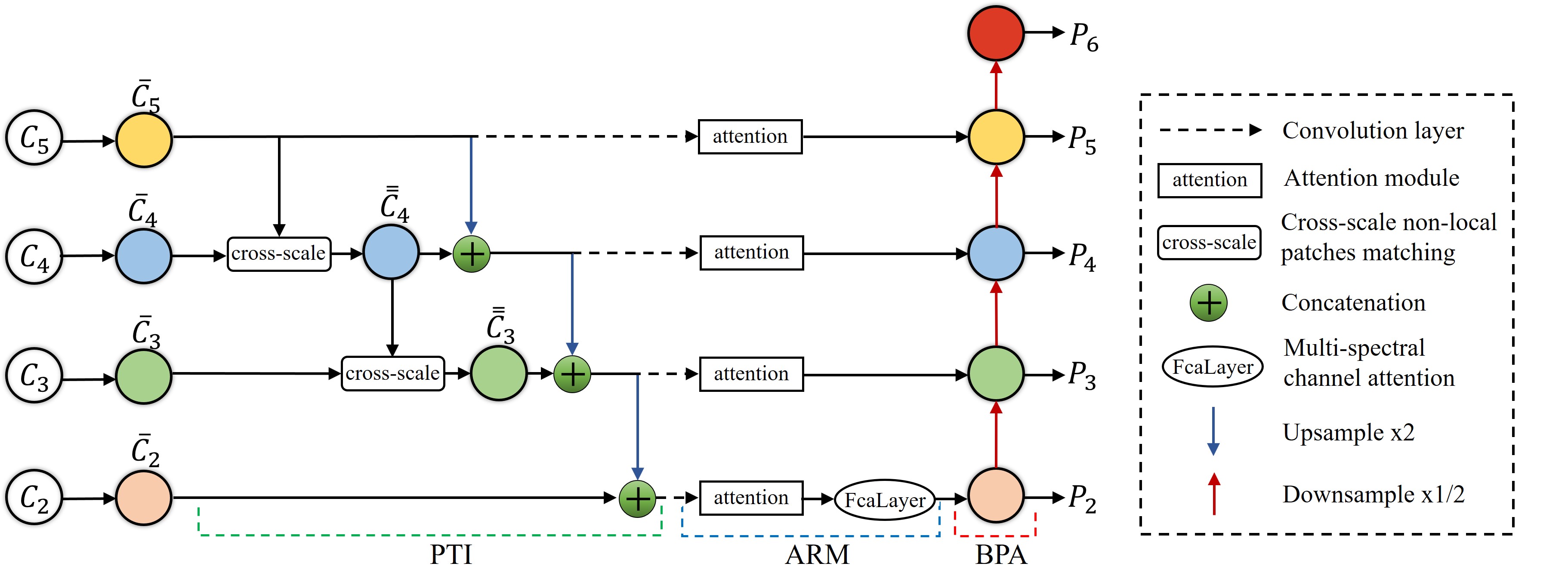
Figure 1: Illustration of RiWFPN. RiWFPN includes progressive top-down interaction module (PTI), attention refinement module (ARM) and bottom-up path augmentation (BPA) three components.

II Related work

II-A Moving Object Segmentation

The traditional multi-motion segmentation method [21, 22, 23, 24] using powerful geometric constraints cluster points of the scene into objects with different motion models. This type of method is at the feature point level instead of instance-level, limited by the model number of the segmentation and has a high computational burden. Some deep-learning-based [25, 26, 27, 28, 29] methods can segment foreground moving objects from the dynamic scene without distinguishing each object instance. MODNet [25] proposes a novel two-stream architecture combining appearance and motion cues, and FuseMODNet proposes a real-time architecture fusing motion information from both camera and LiDAR. More recent approaches [30, 31, 6, 7, 8, 32] have used motion information from optical flow for the instance-level moving object segmentation. The method proposed in [6] discovers different moving objects based on their motion by foreground motion clustering. U²-ONet [32] proposes a novel two-level nested U-structure to learn to segment moving objects and utilizes octave convolution (OctConv) [33] to reduce computational burden. However, these methods are operated under in clear weather conditions, and they have problems inevitably under severe weather conditions. In contrast, RiWNet performs well even in severe weather environments.

II-B Robust Perception in Adverse Weather Conditions

For robust perception in adverse weather environment, some common methods [34, 35, 12, 13, 36, 37] try to obtain the data with various adverse weather effects, and then use these data to train the network to improve the influence of the network on real weather interference. The methods proposed in [13] and [12] propose a Foggy Cityscapes dataset with simulating fog and a RainCityscapes dataset with synthesizing rain streak respectively based on the generic Cityscapes [38] dataset. This type of methods increases the amount of training data and greatly increases the training cost. Recently, some methods [39, 14, 40, 15, 41] regard each weather condition as a new domain, and improve the effect of the network in severe weather conditions based on domain adaptation methods. MS-DAYOLOs [41] performs domain adaptation at multi-layer features from backbone network to generate domain invariant features for YOLOV4 [42]. Due to the addition of additional structures or features, these methods increase the difficulty of network training. Other common methods [9, 43, 16] consider that different sensors perform differently in severe weather conditions and use multi-sensor fusion methods to improve the effect of perception. However, multi-sensor data is often difficult to obtain for cost or scenario constraints. Another possibility [17] is to use the way of video processing and try to compensate the perception error of the current frame by using the image information of the sequence frame. The method proposed in [17] modifies the recurrent units to ensure real-time performance and introduces a robust semantic segmentation using video-segmentation. In the proposed approach, we focus on a new possibility that is to make the network perform robustly in harsh weather conditions by improving its resilience to adverse weather effects through the network’s structural design.

II-C Architecture for Pyramidal Representations

For deep learning-based perception tasks, features from different levels of the pyramid representation are often used. As a basic work, FPN (Feature Pyramid Network) [44] adopts a top-down pyramidal structure to represent multi-scale features. Taking FPN as a baseline, PANet [45] creates a bottom-up path augmentation to much enhance FPN. Different from standard FPN, RFP (Recursive Feature Pyramid) [46] designs extra feedback connections into the bottom-up backbone layers. Feature Pyramid Grids (FPG) [47] represents the feature scale space as a regular grid that combines multi-directional horizontal connections and bottom-up parallel paths. NAS-FPN [48] combines neural architecture search to learn the optimal feature pyramid structure. HRFPN [49, 50] concatenates the upsampled representations from all the backbone layers to augment the high-resolution features and uses average pooling to downsample the concatenated representation for constructing a multi-level representation. To deal with noisy images, OcSaFPN [51] improves the noise-resilient ability of the network itself by increasing the interaction between different frequency components and compressing the redundant information of low frequency components. However, these FPN methods do not consider to deal with the interference caused by bad weather conditions. By using RiWFPN as the neck structure instead of other FPN methods, the performance of our method in severe weather environments can be directly improved.

III Method

Firstly, robust RiWFPN is described, including how to improve the robustness of the network in the interference of weather conditions. Then, the overall structure of RiWNet is introduced, including its inputs and how to learn motion information. The proposed moving instance segmentation dataset considering various weather conditions is introduced at the end of this section.

III-A RiWFPN

III-A1 overview

As shown in Fig. 1, inputs of RiWFPN are the feature maps of four levels $\left\{C_{2},C_{3},C_{4},C_{5}\right\}$ generated by the backbone. It has been demonstrated in the literature that noise in features can be drastically reduced via re-scaling to coarser pyramid level and noisy patches as well as edge patches usually have their corresponding ”clean” patches at coarser image scales of the same relative image coordinates [52]. Inspired by this conclusion, we first perform a progressive top-down interaction module to enhance the feature map of each scale. This module borrows low-scale “clean“ information through cross-scale non-local patches matching, and increases the spread of clean information while introducing more spatial and semantic information through the concatenation of adjacent-scale feature maps. And then we use an attention refinement module to refine the abundant information for highlighting significant features for specific scales, and to enhance low-frequency structural information. Finally, the bottom-up path augmentation is used to strengthen the propagation of high-scale refined feature maps and optimize the feature maps of the entire network.

III-A2 progressive top-down interaction module

Inspired by [52] and [53], cross-scale non-local patches matching of adjacent scales is used to introduce “clean” information on lower scales (especially better edge information) into higher scales. Cross-scale non-local patches matching is first performed on feature maps of adjacent scales $\left\{\overline{C}_{4},\overline{C}_{5}\right\}$, bringing “clean” recurrence information on lower scales into current scales to obtain $\left\{\overline{\overline{C}}_{4}\right\}$ which is the ”cleaner” version of $\left\{C_{4}\right\}$. Recursively, the feature map $\left\{\overline{\overline{C}}_{4}\right\}$ is then subjected to cross-scale non-local patches matching operation with $\left\{\overline{C}_{3}\right\}$. The feature map $\left\{\overline{C}_{2}\right\}$ with the highest scale is larger in size. In order to avoid adding too much computational overhead, no cross-scale matching operation is performed on $\left\{\overline{C}_{2},\overline{\overline{C}}_{3}\right\}$.

Formally, given two input feature maps $F$ and $G$ of adjacent scales (the scale of $F$ is greater than $G$), cross-scale non-local patches matching operation is defined as:

$$y^{i}=\frac{1}{\sigma(F,G)}\sum_{j}\phi(F^{i}_{\delta(r)},G^{j}_{\delta(r)})\theta(G^{j}),$$ (1)

where $i$, $j$ are index on the input $F$ and input $G$ as well as output $y$. The function $\phi$ computes pair-wise affinity between two input features. $\theta$ is a feature transformation function that generates a new representation of $G^{j}$. The output response $y^{i}$ obtains information from all features through explicitly summing over all positions and is normalized by a scalar function $\sigma(F,G)$. The neighborhood is specified by $\delta(r)$. $r\times r$ patches are extracted from the feature map. For $\phi$, we use embedded Gaussian[54] as:

$$\phi(F^{i},G^{j})=e^{f(F^{i})^{T}g(G^{j})},$$ (2)

The scalar function $\sigma(F,G)$ is set as:

$$\sigma(F,G)=\sum_{j\in G}\phi(F^{i},G^{j})$$ (3)

where, $f(F^{i})=W_{f}F^{i}$ and $g(G^{j})=W_{g}G^{j}$. we use a simple linear embedding for the function $\theta$: $\theta=W_{\theta}G^{j}$.

Then, the progressive top-down concatenation is performed. For each scale except the lowest scale of the pyramid, the current scale feature map and upsampled feature maps from its previous scale are concatenated. Through this progressive concatenation method, more low-level features are integrated and the fusion of features of different scales is promoted, to obtain more spatial and semantic information. At the same time, this concatenation interaction between different scales improves the propagation of “cleaner” feature maps obtained by cross-scale patch matching, and optimizes feature maps at various scales. Inspired by the conclusion proved by [51] that the transmission of the information at different frequency components can enhance noise-resilient performance of the network, this top-down progressive concatenation is also used to increase the interaction between different scales. In this way, the network’s resilience to noise such as rain and fog is improved.

III-A3 attention refinement module

The abundant feature maps after concatenation have vast spatial and channel aggregation information of multi-scale concatenated feature maps, but making scale features of targets not significant enough. For feature map $\left\{\overline{C}_{5}\right\}$ and the three feature maps after concatenation, convolutional block attention module (CBAM) [55] is used to fuse multi-scale feature maps for highlighting significant features of specific scales. CBAM (as shown in Fig. 2) weights in dimensions of scale and spatial respectively by introducing channel and spatial attention mechanisms. Channel attention attempts to selecting feature maps of suitable scales and spatial attention concentrates on finding salient portions in a feature map. Through this operation, multiscale feature maps are refined adaptively by CBAM, to emphasize the prominent features of specific scales and pay more attention to specific scales for multi-scale segmentation.

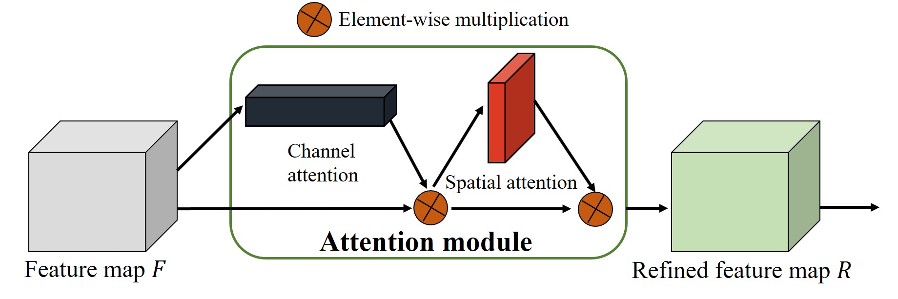
Figure 2: Overview of convolutional block attention module (CBAM) [55]. CBAM introduces channel and spatial attention mechanisms.

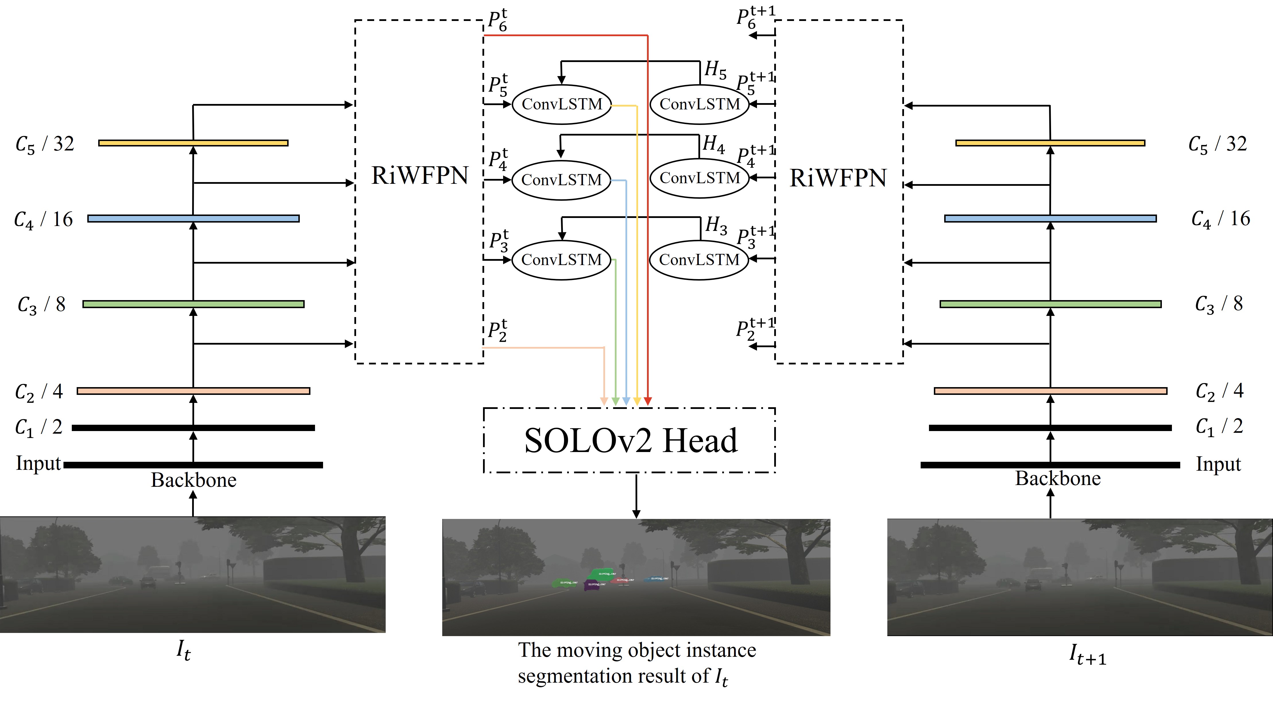
Figure 3: Overview of RiWNet. The input of RiWNet is two adjacent frames of RGB images $I_{t},I_{t+1}$, and the output is the segmentation result of the moving object instance in the current frame $I_{t}$. The RiWFPN used is introduced in Section III-A.

The existing attention model using GAP as pre-processing method only uses the information equivalent to the lowest frequency of the DCT (Discrete Cosine Transform), while discarding much useful information equivalent to other frequency of the DCT, as mentioned in [56]. Therefore, the multi-spectral attention module Fcalayer [56] is proposed to exploit the information from different frequency components of the DCT, to making full use of the information in the attention mechanism more efficiently. Based on the conclusion of [52] that noise levels drop dramatically at coarser image scales, we use Fcalayer to optimize the highest-scale feature map $\left\{C_{2}\right\}$ that we think is the most noise levels. Fcalayer embeds different frequency information, and selects Top-k highest performance frequency components in each frequency. In addition, the frequency components selected by the Fcalayer selection mechanism is usually more biased towards selecting low-frequency, as proved in [56]. Therefore, the highest-scale feature map optimized by Fcalayer can have rich low-frequency information to improve the structural information of the network. Better structural information helps improve the network’s resilience to the weather interference such as rain and fog.

III-B RiWNet

As illustrated in Fig. 3, the overall structure of RiWNet is introduced. First, given a pair of RGB frames at adjacent time $I_{t},I_{t+1}\in\mathbb{R}^{h\times w\times 3}$, we take ResNet101 [57] as the backbone. $\left\{P_{2}^{t},P_{3}^{t},P_{4}^{t},P_{5}^{t},P_{6}^{t}\right\}$ and $\left\{P_{2}^{t+1},P_{3}^{t+1},P_{4}^{t+1},P_{5}^{t+1},P_{6}^{t+1}\right\}$ respectively represent feature levels generated by the proposed RiWFPN (in Section III-A) at time $t$ and $t+1$. Then the three feature maps $\left\{P_{3}^{t+1},P_{4}^{t+1},P_{5}^{t+1}\right\}$ at time $t+1$ are respectively input into a ConvLSTM structure [19], and three feature maps $\left\{H_{3},H_{4},H_{5}\right\}$ are output. Considering that the large size of $\left\{P_{2}^{t+1}\right\}$ bring a lot of computational burden, and that $\left\{P_{6}^{t+1}\right\}$ contains less information, the feature maps of three levels $\left\{P_{3}^{t+1},P_{4}^{t+1},P_{5}^{t+1}\right\}$ are selected. At the same time, we also experimentally proved (in Section IV-D2) that using the feature maps of three levels $\left\{P_{3}^{t+1},P_{4}^{t+1},P_{5}^{t+1}\right\}$ is better than using only the feature map $\left\{P_{2}^{t+1}\right\}$. Three feature maps $\left\{P_{3}^{t},P_{4}^{t},P_{5}^{t}\right\}$ and three feature maps $\left\{H_{3}^{t},H_{4}^{t},H_{5}^{t}\right\}$ at time $t+1$ are respectively used as the input feature map and hidden layer feature map of the ConvLSTM structure for processing. As mentioned in  [17], ConvLSTMs capture the temporal image information well. In this way, the ConvLSTM is used to introduce the information at time $t+1$ into the feature map at time $t$ to realize the processing of temporal information and guide the network to learn the motion information in adjacent temporal images in addition to appearance information. Finally, the three feature maps after processed by the ConvLSTM structure and the two feature maps $\left\{P_{2}^{t},P_{6}^{t}\right\}$ at time $t$ are used as the input of SOLOv2 Head [18] to obtain the result of moving instance segmentation.

III-C VKITTI-moving

To train and verify our deep model for robust performance in weather disturbances, we propose a publicly available moving instance segmentation dataset, called VKITTI-moving by generating motion masks annotations from a large driving dataset-VKITTI (Virtual KITTI) [20] (as shown in Fig. 4). VKITTI dataset consists of 5 tracking sequence and provides these sequences after modified weather conditions (e.g. fog, rain, sunset, morning and overcast). Although VKITTI contains left and right camera images under different camera configurations (e.g. rotated by $30\degree$), they are all images from different perspectives collected in the same scene, we only take ”15-deg-left-Camera_0” collected by the left camera rotated 15 degrees. To generate motion masks from VKITTI, we take the instance segmentation groundtruth mask, manually select and retain masks belonging to moving objects. In addition to the background, VKITTI-moving has only one category: moving_car, the category of all labeling instance masks is moving_car. VKITTI-moving considers different weather conditions including rain, fog, sunset, morning and overcast in the same scene. It contains 4650 images (shown in TABLE I), and is divided to three subsets: Fog, Rain and Illumination (including sunset, morning and overcast). The size of the image is (1242, 375). For quantifying the performance, we use the precision (P), recall (R), and F-measure(F), as defined in [58], as well as the mean intersection over union (IoU) for the evaluation metrics.

TABLE I: Introduction of the VKITTI-moving dataset

Subset		Image quantity in training set	Image quantity in testing set	Instances
Fog		660	270	2550
Rain		660	270	2550
Illumination	sunset	660	270	2550
	morning	660	270	2550
	overcast	660	270	2550

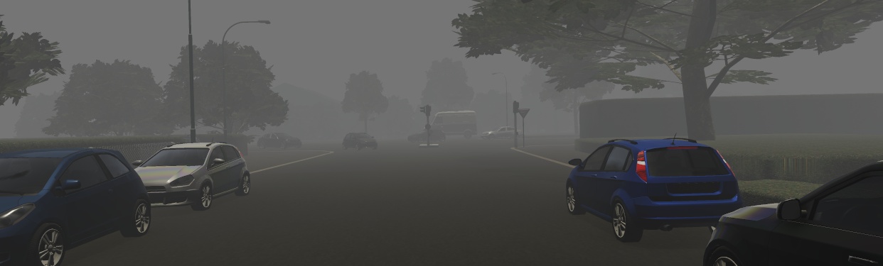
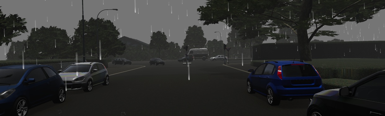
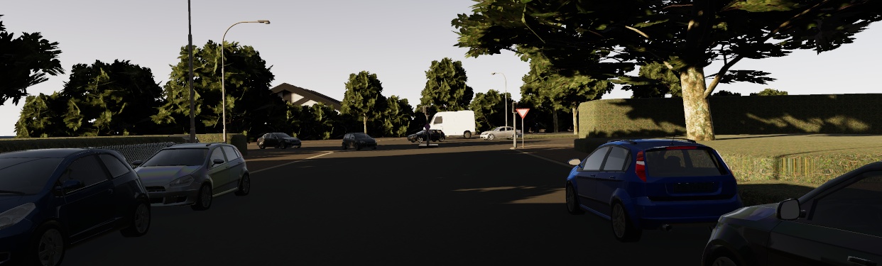
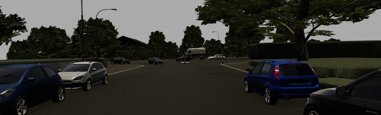
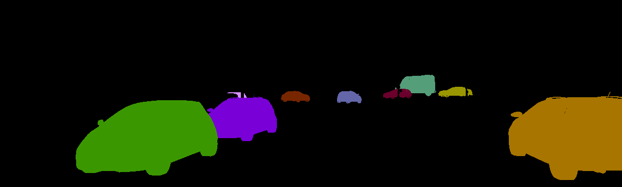
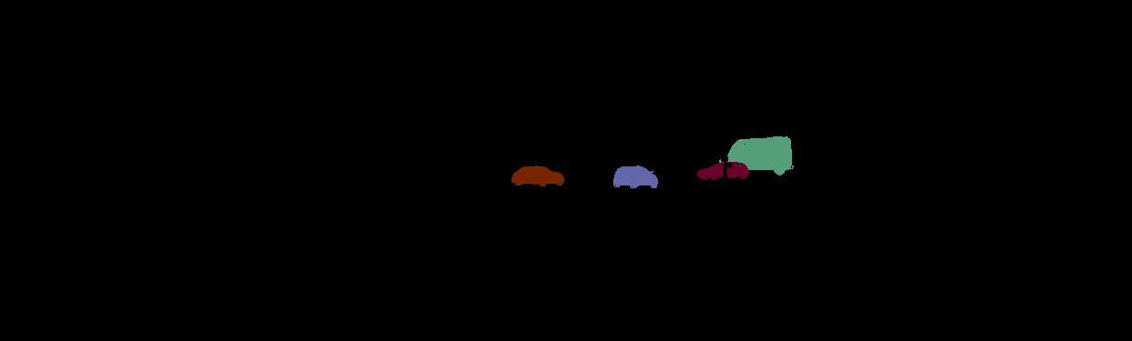
Figure 4: The example image of VKITTI-moving. (a) Fog image. (a) Rain image. (c) Sunset image. (d) Overcast image. (e) Instance segmentation labels of VKITTI. (f) Moving instance segmentation labels of our VKITTI-moving.

IV Experiments

IV-A Datasets

We evaluated the proposed method on several benchmark datasets: our VKITTI-moving (in Section III-C), FBMS (Freiburg–Berkeley Motion Segmentation) dataset [58], YTVOS (YouTube Video Object Segmentation) dataset [59]. FBMS is a widely used moving object segmentation dataset, and many methods are tested on this dataset. We used a corrected version [60] linked from FBMS’s website because the original FBMS has a lot of annotation errors. The YTVOS dataset is a challenging video object segmentation dataset containing many objects that are difficult to segment, such as tiny objects, and camouflaged objects. For testing moving object segmentation, we used the moving object version of YTVOS, called YTVOS-moving proposed in  [7].

IV-B Implementation Details

For the experiments, we take ResNet101 pretrained on ImageNet [61] as the backbone. As for VKITTI-moving dataset, the longer image side is 1242. We use scale jitter for the shorter image side, and it is randomly sampled from 800 to 640 pixels. For FBMS and YTVOS, the longer image side is set to 1242, and the shorter image side is randomly sampled from 512 to 352 pixels. RiWNet is trained with stochastic gradient descent (SGD). Its initial learning rate is 0.001 and its hyperparameters are set as follows: momentum=0.9, weight_decay=0.00001. We train for 40 epochs using a batch size of 2. The experiments are all conducted on a single NVIDIA Tesla V100 GPU with 16GB memory, along with the PyTorch 1.4.0 and Python 3.7. In the VKITTI-moving dataset, RiWNet can run end-to-end at a speed of about 5HZ in this configuration. The results are evaluated using the mean intersection over union (IoU), precision (P), recall (R), and F-measure (F). Source code and the models as well as VKITTI-moving dataset will be made public in https://github.com/ChenjieWang/RiWNet upon the publishment of the paper.

IV-C Visualization of Feature Maps

To fully demonstrate how RiWNet enhance the feature map, we visualize related processing results of the feature map $\left\{P_{2}^{t}\right\}$ in our method. First, we average the values of all channels on each pixel coordinate (i, j) to obtain the mean feature map. For comparison, we also calculated the mean feature map of RiWNet using other FPN structures (including HRFPN and NASFPN) instead of RiWFPN. The quantitative results (in Section IV-E) prove that these two FPN structures are the best two structures in weather conditions other than RiWFPN, so we compare our RiWFPN with these two structures. We visualize these mean feature maps in Fig. 5. In comparison, the feature maps of all channels of our RiWFPN are more consistent, the mean feature map has better low-frequency structure information, and the target object is more significant.

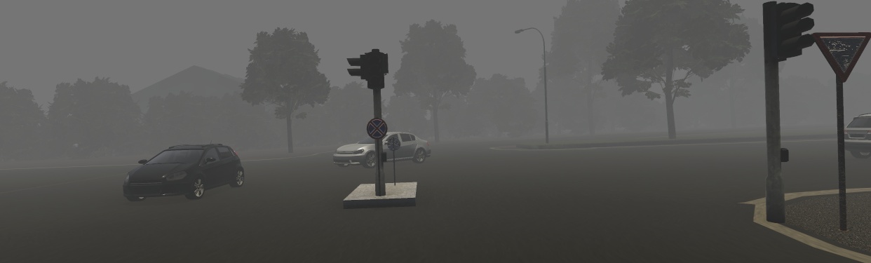
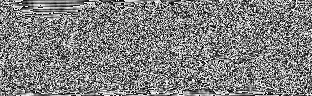
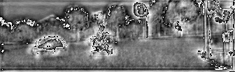
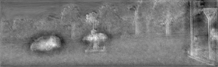
Figure 5: Comparison of visualization of the mean feature map obtained using different FPN structures. (a) Original image with fog. (a) The mean feature map obtained with NASFPN. (c) The mean feature map obtained with HRFPN. (d) The mean feature map obtained with RiWFPN.

At the same time, in order to prove that the consistency of our method is not due to the decrease in the amount of information in each channel and the increase in the duplication of information in each channel. We calculate the correlation coefficient between the feature map of each channel and the mean feature map respectively. Meanwhile, we also calculate the correlation coefficient between every two channels in all channels. The correlation coefficient $corr$ is defined as:

$$corr=\frac{\sum_{i}\sum_{j}(F^{n}_{ij}-\overline{F^{n}})(mF_{ij}-\overline{mF})}{\sqrt{(\sum_{i}\sum_{j}(F^{n}_{ij}-\overline{F^{n}})^{2})(\sum_{i}\sum_{j}(mF_{ij}-\overline{mF})^{2})}}.$$ (4)

The comparison of correlation coefficients are shown in Fig. 6 and Fig. 7. It is interesting to point out, the correlation coefficient between each channel and the average channel or between every two channels of RiWFPN is generally lower. It indicates that the use of RiWFPN introduces more information. Combined with the results in Fig. 5, RiWFPN has introduced more information while enhancing the consistency of information in different channels. In general, RiWFPN enhances the low-frequency structure information in the network, which is more conducive to maintaining robustness in adverse weather interference.

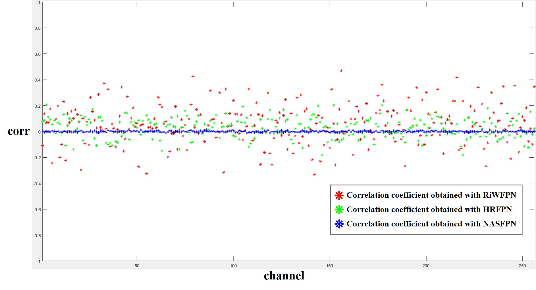
Figure 6: Comparison of correlation coefficients obtained using different FPN structures. The correlation coefficient distribution of RiWFPN is more discrete.

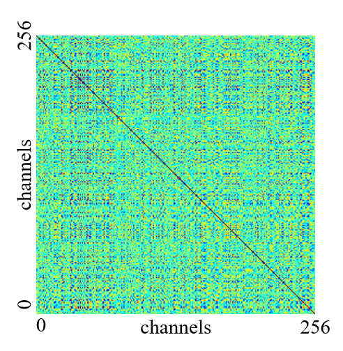
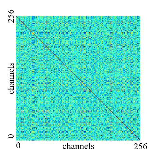
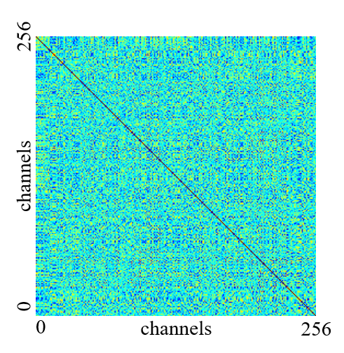
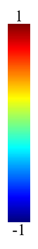
Figure 7: (a) Visualized image of Correlation coefficient of NASFPN. (b) Visualized image of Correlation coefficient of HRFPN. (c) Visualized image of Correlation coefficient of RiWFPN. (d) Colormap indicating that the correlation coefficient is from -1 to 1.

We also calculated the correlation coefficient between the feature vector composed of each channel value of each pixel coordinate (i, j) and the reference pixel coordinate feature vector. We manually selected two reference pixel locations on the target moving object, and two reference pixel locations on the background. The results are shown in Fig. 8. The reference pixel coordinates in Fig. 8 and Fig. 8 are located on the target moving object. It can be seen that the feature map of RiWFPN shows better correlation within the target moving object class than HRFPN. In particular, there is an object that only appears partly on the far right, our method still shows good intra-class correlation of moving objects. Meanwhile, the difference between the target moving object class and the background class in RiWFPN is larger than NASFPN. Therefore, in adverse weather scenarios, RiWNet increases the intra-class correlation of moving objects and minimizes intra-class variance, while enlarging inter-class difference, making the objects easier to segment.

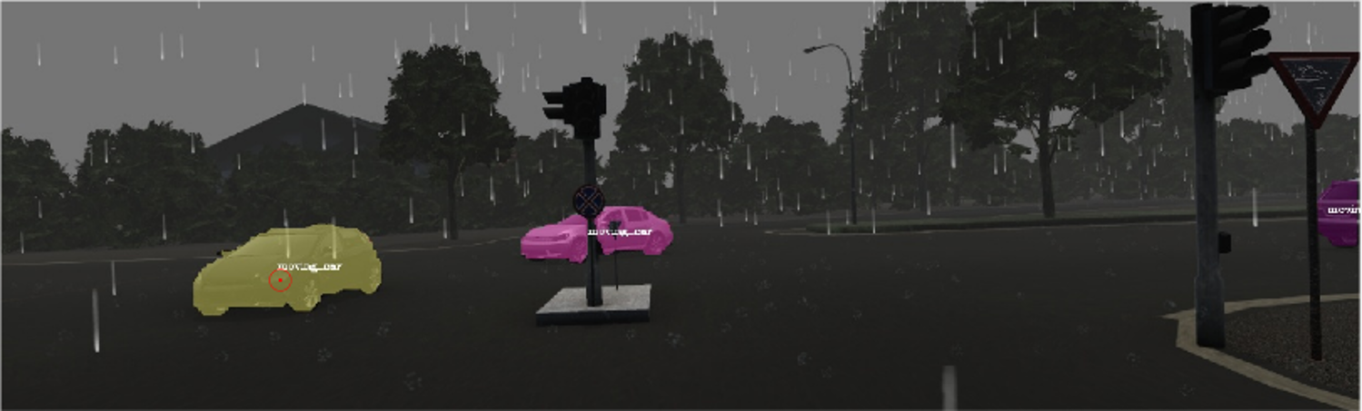
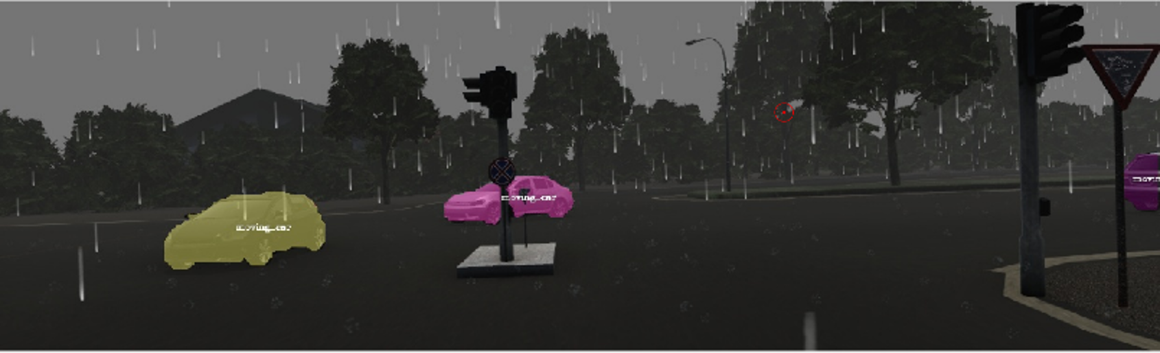
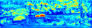
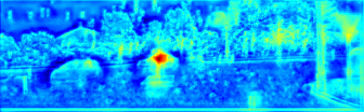
Figure 8: The correlation coefficient between the feature vector of each pixel coordinate and the reference pixel coordinate feature vector. The reference pixel position is the center of the red circle in the figure. The reference pixel coordinates in (a) and (b) are located on the target moving object. The reference pixel coordinates in (c) and (d) are located on the background. (a-d) Original image with rain. (e-h) Visualized image of Correlation coefficient of NASFPN. It can be seen that a large number of backgrounds are highly correlated with target objects. NASFPN has good intra-class correlation, but poor inter-class differences. (i-l) Visualized image of Correlation coefficient of HRFPN. It can be seen that the correlation within the target object class is not high. HRFPN has good inter-class differences, but poor intra-class correlation. (m-p) Visualized image of Correlation coefficient of RiWFPN. RiWFPN has good intra-class correlation and inter-class differences.

IV-D Ablation Studies

All the results of ablation experiments are performed on VKITTI-moving dataset and obtained by mixing the training sets of three subsets of Fog, Rain, and Illumination together for training, and then evaluating on the testing sets of these three subsets respectively.

IV-D1 Ablation Studies on RiWFPN

We verify the effectiveness of each component of RiWFPN, including progressive top-down interaction module (PTI), attention refinement module (ARM) and bottom-up path augmentation (BPA) three components. The results are shown in TABLE II. When there is no attention optimization module (ARM), abundant aggregation information makes the target not significant enough and difficult to discover, so the recall metric is low. The combination of PIL and ARM greatly improves the effect of the network in weather interference. At the same time, BPA also has a positive effect on network accuracy. This ablation study verify our claim of how RiWFPN maintains robustness in weather interference discussed in Section III-A.

IV-D2 Ablation Studies on RiWNet

As discussed in Section III-B, in order to reduce the computational burden, we only used the feature maps of 3, 4, and 5 levels into ConvLSTM structure for processing. This ablation study is performed to demonstrate the effectiveness of this design. As shown in TABLE III, using the feature maps of 3, 4, and 5 levels achieves better results than the feature map of only 2 level, while both methods reduce the computational cost.

IV-E Comparison between RiWFPN and other state-of-the-art FPN structure

In order to compare the robustness of RiWFPN and other FPN structures in weather interference, we conduct a series of experiments using RiWNet with different FPN structures. In TABLE IV, these are the results obtained by training on the training sets of three subsets of Fog, Rain, and Illumination respectively instead of mixing these three subsets to train. It can be seen that our method obtains the best results in all four metrics in Rain. As a contrast, the results in TABLE V obtained by mixing the training sets of three subsets of Fog, Rain, and Illumination together for training, and then evaluating respectively. It is shown that RiWFPN obtains the best results on all metrics in the three cases of Fog, Rain, and Illumination, which is much better than other FPN methods. This also proves that our method does not need to train only one weather pattern at a time like other methods. It can train the data of multiple weather patterns at one time and still perform better in each weather condition. The qualitative results of RiWNet in VKITTI-moving are shown in Fig. 9.

TABLE II: Ablation Studies on RiWFPN. PTI means progressive top-down interaction module, ARM means attention refinement module and BPA means bottom-up path augmentation.

				Fog				Rain				Illumination
	PTI	ARM	BPA	R	P	F	IoU	R	P	F	IoU	R	P	F	IoU
RiWNet + RiWFPN	$\surd$	$-$	$\surd$	67.8544	77.1949	69.2525	61.0120	67.2736	77.4963	68.0752	61.4972	65.1344	76.9296	67.3246	58.8871
RiWNet + RiWFPN	$-$	$\surd$	$\surd$	69.0867	78.2304	71.3624	63.0018	69.0227	77.8654	71.2289	63.2614	66.6008	78.1500	69.6959	60.9981
RiWNet + RiWFPN	$\surd$	$\surd$	$-$	71.7185	78.0656	73.4864	64.9776	71.8159	78.2153	73.5866	65.2354	69.3519	77.6455	71.6561	62.8545
RiWNet + RiWFPN	$\surd$	$\surd$	$\surd$	72.1911	78.7783	73.9263	65.4380	72.3076	78.6134	74.0181	65.7298	70.3866	78.5284	72.7195	64.0795

TABLE III: Ablation Studies on RiWNet.

		Fog				Rain				Illumination
	Levels used	R	P	F	IoU	R	P	F	IoU	R	P	F	IoU
RiWNet + RiWFPN	only 2	70.3519	77.3152	71.7914	63.0688	70.1986	77.0337	71.3784	63.0978	68.5441	76.8563	70.4466	62.0619
RiWNet + RiWFPN	3 4 5	72.1911	78.7783	73.9263	65.4380	72.3076	78.6134	74.0181	65.7298	70.3866	78.5284	72.7195	64.0795

TABLE IV: Comparison between RiWFPN and other state-of-the-art FPN structure. These are the results obtained by training on the training sets of three subsets of Fog, Rain, and Illumination respectively and testing on the testing sets of three subsets respectively.

	Fog				Rain				Illumination
	R	P	F	IoU	R	P	F	IoU	R	P	F	IoU
RiWNet + FPN	64.3160	73.2833	66.7664	55.9594	63.9901	75.4874	67.4494	57.7026	66.0082	75.5300	68.8863	59.4433
RiWNet + PAFPN	66.5676	76.0739	69.3792	59.4991	69.4217	77.4146	71.5948	62.3430	66.9639	75.7860	69.4689	60.1148
RiWNet + FPG	67.2878	75.9978	70.0873	60.9971	69.1623	78.0225	72.1775	62.7113	64.4351	75.0395	66.6059	57.6032
RiWNet + RFP	62.7925	73.0408	66.0832	55.4460	67.2318	76.6518	69.4800	59.8921	68.6223	76.8415	71.0885	61.8353
RiWNet + NASFPN	71.0906	79.9115	73.8307	63.4506	65.0104	74.0085	67.1104	57.1253	66.1716	81.4152	70.6771	59.8121
RiWNet + HRFPN	71.1792	78.8042	73.6642	64.7437	68.7144	78.2312	71.7578	62.3309	67.3544	76.5178	69.8822	60.5343
RiWNet + RiWFPN	68.7513	76.6170	70.9883	61.6493	70.3652	79.6420	73.3892	64.5407	68.0239	77.0120	70.2856	61.2063

Best results are highlighted in $\rm{\color[rgb]{1,0,0}red}$ with second best in $\rm{\color[rgb]{0,0,1}blue}$.

TABLE V: Comparison between RiWFPN and other state-of-the-art FPN structure. These results are obtained by mixing the training sets of three subsets of Fog, Rain, and Illumination together for training, and then evaluating respectively.

	Fog				Rain				Illumination
	R	P	F	IoU	R	P	F	IoU	R	P	F	IoU
RiWNet + FPN	67.1934	75.9910	69.6194	60.2508	68.0027	76.0370	70.2864	60.8403	64.9424	75.2914	67.6752	57.9608
RiWNet + PAFPN	69.8223	76.8181	71.9257	63.1057	68.7693	76.0352	70.9302	62.0728	67.0133	75.7977	69.3109	60.0565
RiWNet + FPG	66.0783	76.4919	68.4716	59.5495	65.5916	76.6606	68.3113	59.3429	64.4074	76.6008	67.3842	58.0600
RiWNet + RFP	69.6138	76.6718	71.8139	62.5276	68.9629	75.2874	70.6670	61.2696	67.6848	75.2554	69.7875	60.4021
RiWNet + NASFPN	69.3932	77.6686	71.4881	62.7676	68.8042	78.0920	71.0696	62.1259	64.0359	77.1758	67.1837	57.5821
RiWNet + HRFPN	70.9928	77.4495	72.9079	63.8511	70.4500	76.8053	72.2372	63.2345	67.2949	75.7817	69.6622	60.2593
RiWNet + RiWFPN	72.1911	78.7783	73.9263	65.4380	72.3076	78.6134	74.0181	65.7298	70.3866	78.5284	72.7195	64.0795

Best results are highlighted in $\rm{\color[rgb]{1,0,0}red}$ with second best in $\rm{\color[rgb]{0,0,1}blue}$.

IV-F Comparison with Prior Works

IV-F1 FBMS

FBMS is a widely used moving object segmentation dataset, and RiWNet is evaluated on this dataset against multiple prior works. RiWNet is evaluated on testing set of the standard FBMS using the model trained from training set mixed by FBMS and YTVOS. The results are shown in TABLE VI. RiWNet performs the best in precision and F-measure and outperforms other methods by over 3.7% and 1.6%, respectively. In terms of recall, it also outperforms most methods and outperforms other methods except U²-ONet [32] by over 0.9%. The qualitative results are shown in Fig. 9.

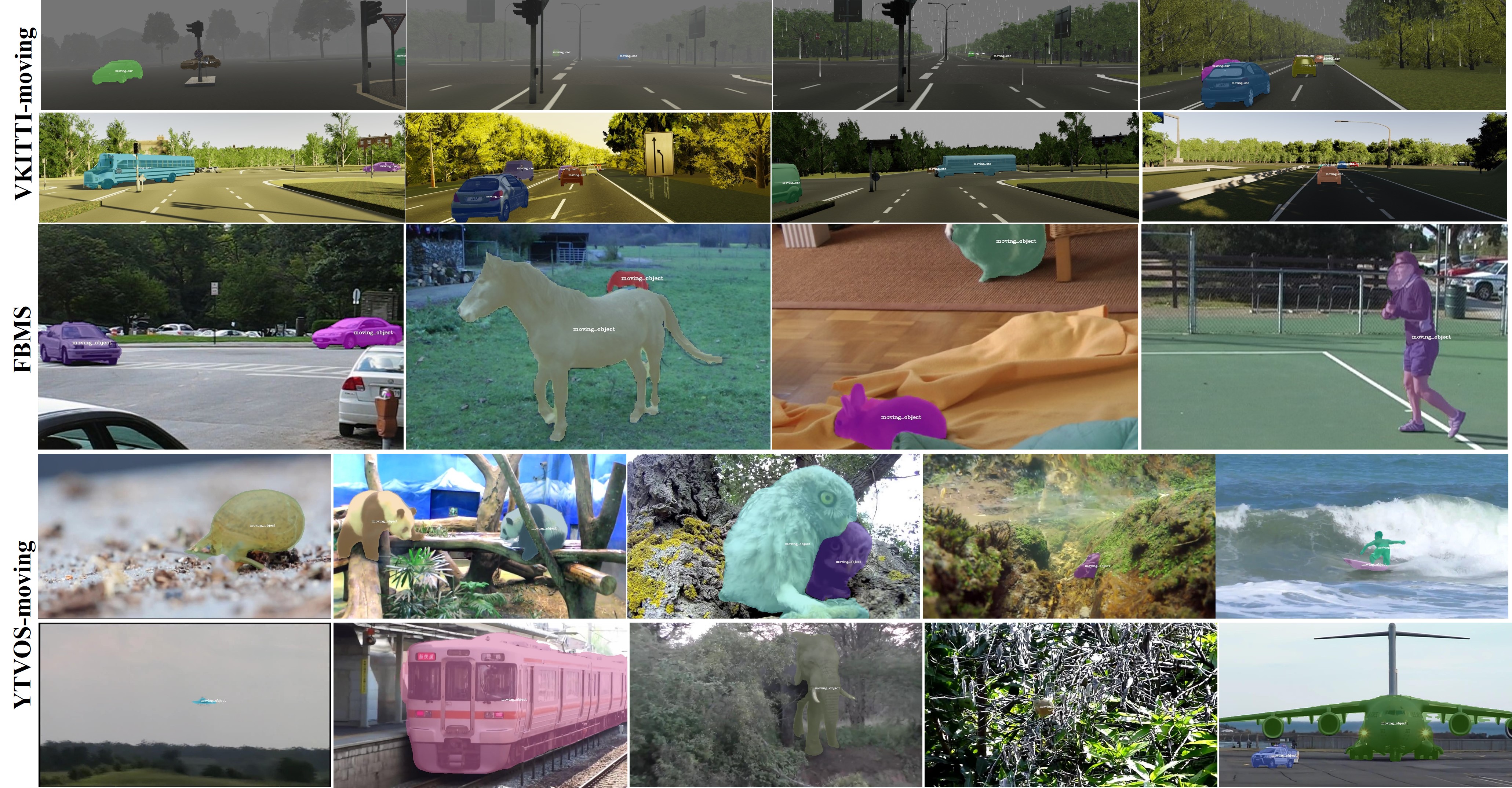
Figure 9: Qualitative results for three datasets.

TABLE VI: FBMS results using the official metric

	Multi-object Motion Segmentation
	R	P	F	IoU
CCG [31]	63.07	74.23	64.97	–
STB [30]	66.53	87.11	75.44	–
OBV [6]	66.60	75.90	67.30	–
TSA [7]	80.40	88.60	84.30	–
U2-ONet [32]	83.10	84.80	81.84	79.70
RiWNet	81.36	92.30	85.99	76.71

Best results are highlighted in $\rm{\color[rgb]{1,0,0}red}$ with second best in $\rm{\color[rgb]{0,0,1}blue}$.

IV-F2 YTVOS-moving

RiWNet is further evaluated on the YTVOS-moving testing set using the model trained from the YTVOS-moving training set, as defined in [7]. The results are listed in TABLE VII. RiWNet performs the best in recall, precision and F-measure, and outperforms U²-ONet [32] and TSA [7] by over 4.1% in precision and over 3.4% in F-measure. The qualitative results are shown in Fig. 9.

TABLE VII: Results for the YouTube Video Object Segmentation (YTVOS)-Moving dataset.

	Multi-Object Motion Segmentationn
	R	P	F	IoU
TSA [7]	66.40	74.50	68.30	$–$
U2-ONet [32]	70.56	74.64	69.93	65.67
RiWNet	70.73	79.80	73.35	65.02

IV-G Applications

Main applications of RiWNet are dynamic Visual SLAM or visual-LiDAR fusion odometry/SLAM as well as 3D dense mapping. Here we show the effectiveness of RiWNet, adding RiWNet as a processing module to segment moving objects for keyframes in our previous work called DV-LOAM [62] of visual-LiDAR fusion SLAM. In DV-LOAM, because the relative transformation of the camera and laser is known, just using the image of the moving object segmentation result can handle the point cloud of the entire Visual LiDAR fusion SLAM. We only use masks to remove effectively all visual feature points and point clouds belonging to moving objects and no further operations have been employed. We conduct experiments on the Sequence 04 in KITTI odometry benchmark [63] because this sequence contains more moving cars. Because RiWNet runs in another thread and only processes key frames, the experimental results show that the adding of RiWNet (running about 5HZ) does not affect the real-time operation of DV-LOAM.

IV-G1 visual-LiDAR fusion odometry/SLAM

We compare the improved DV-LOAM after adding RiWNet to standard DV-LOAM in TABLE VIII. The results show that estimating odometry using the improved DV-LOAM are higher precision than standard DV-LOAM.

TABLE VIII: Comparison of odometry results.

	Approach
	DV-LOAM	DV-LOAM+RiWNet
Sequence 04	0.30/0.61	0.26/0.56

Relative errors averaged over trajectories in Sequence 04: relative rotational error in degrees per 100 m / relative translational error in %.

IV-G2 3D Mapping

In Fig. 10, We show the final point cloud maps generated with and without using moving object masks respectively. As shown in Fig. 10, a polluted point cloud map containing moving objects is generated due to the existence of moving objects. This polluted map is likely to reduce the accuracy of loop closure detection and the effect of motion planning. By using our RiWNet to handle moving objects, the static structure are more clearly observable.

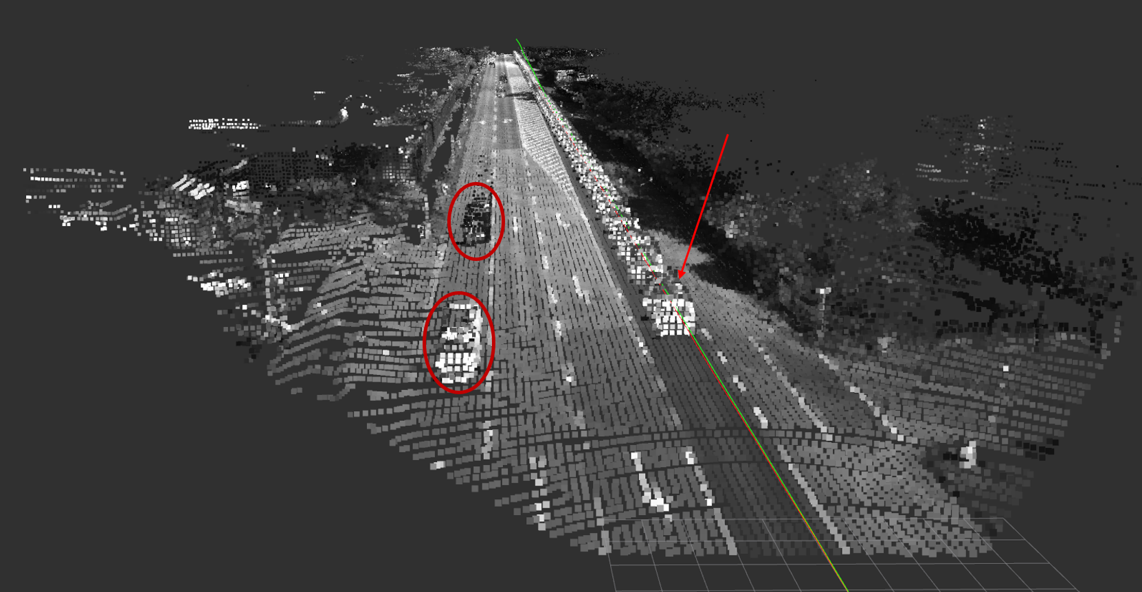
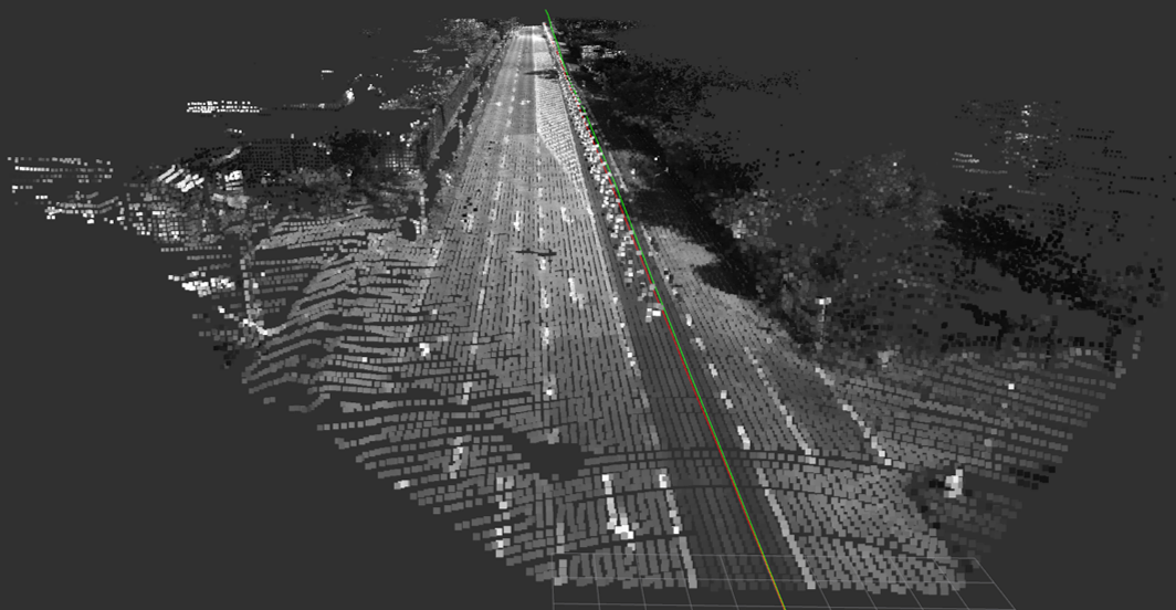
Figure 10: Generated point cloud maps on Sequence 04. (a) shows the result without using moving object masks. (b) shows the result with using moving object masks for removing point cloud predicted as moving. In (a), the red ellipse and red arrow in the figure indicate the moving objects included in the final map. In (b), the point cloud of moving objects is almost removed. There is a certain point cloud of moving objects at the place pointed by the red arrow, because there is a certain region at the edge of the object that is difficult to segment.

V Conclusion

The effect of moving object segmentation usually decrease enormously in adverse weather conditions as compared to good weather conditions. In this paper, we firstly propose a novel RiWFPN combining a progressive top-down interaction and attention refinement module to strengthen the low-frequency structure information of the network. Compared with other FPN structures, using RiWFPN as a neck structure can improve the robustness of the network in degrading weather conditions. We then extend SOLOV2 to learn temporal motion information and propose a novel end-to-end moving object instance segmentation network, called RiWNet. RiWNet uses a pair of adjacent RGB frames as inputs and performs robustly in different weather environments by integrating RiWFPN. We construct a moving object instance segmentation dataset considering different weather conditions for verifying the effectiveness of the method. Experimental results fully demonstrate how RiWNet enhance the feature map to improve the robustness of the network in the interference of weather conditions. We also show that RiWNet achieves state-of-the-art performance in some challenging datasets, especially in harsh weather scenarios.

In the near future, we consider incorporating RiWNet to our previous work: a stereo dynamic visual SLAM system [2], as the module of moving object segmentation. We will use RiWNet to segment moving objects in key-frames of SLAM and propose a real-time end-to-end dynamic SLAM be capable of estimating simultaneously global trajectories of the camera and moving objects.

References

- [1] M. Runz, M. Buffier, and L. Agapito, “Maskfusion: Real-time recognition, tracking and reconstruction of multiple moving objects,” in 2018 IEEE International Symposium on Mixed and Augmented Reality (ISMAR), 2018, pp. 10–20.
- [2] C. Wang, B. Luo, Y. Zhang, Q. Zhao, L. Yin, W. Wang, X. Su, Y. Wang, and C. Li, “Dymslam: 4d dynamic scene reconstruction based on geometrical motion segmentation,” IEEE Robotics and Automation Letters, vol. 6, no. 2, pp. 550–557, 2021.
- [3] D. Ferguson, M. Darms, C. Urmson, and S. Kolski, “Detection, prediction, and avoidance of dynamic obstacles in urban environments,” in 2008 IEEE Intelligent Vehicles Symposium, 2008, pp. 1149–1154.
- [4] B.-H. Chen and S.-C. Huang, “An advanced moving object detection algorithm for automatic traffic monitoring in real-world limited bandwidth networks,” IEEE Transactions on Multimedia, vol. 16, no. 3, pp. 837–847, 2014.
- [5] D. Ferguson, T. M. Howard, and M. Likhachev, “Motion planning in urban environments: Part i,” in 2008 IEEE/RSJ International Conference on Intelligent Robots and Systems, 2008, pp. 1063–1069.
- [6] C. Xie, Y. Xiang, Z. Harchaoui, and D. Fox, “Object discovery in videos as foreground motion clustering,” in Proceedings of the IEEE Conference on Computer Vision and Pattern Recognition, 2019, pp. 9994–10 003.
- [7] A. Dave, P. Tokmakov, and D. Ramanan, “Towards segmenting anything that moves,” in Proceedings of the IEEE International Conference on Computer Vision Workshops, 2019, pp. 0–0.
- [8] S. Muthu, R. Tennakoon, T. Rathnayake, R. Hoseinnezhad, D. Suter, and A. Bab-Hadiashar, “Motion segmentation of rgb-d sequences: Combining semantic and motion information using statistical inference,” IEEE Transactions on Image Processing, vol. 29, pp. 5557–5570, 2020.
- [9] A. Pfeuffer and K. Dietmayer, “Robust semantic segmentation in adverse weather conditions by means of sensor data fusion,” in 22th International Conference on Information Fusion, FUSION 2019, Ottawa, ON, Canada, July 2-5, 2019. IEEE, 2019, pp. 1–8. [Online]. Available: https://ieeexplore.ieee.org/document/9011192
- [10] M. J. Mirza, C. Buerkle, J. Jarquin, M. Opitz, F. Oboril, K.-U. Scholl, and H. Bischof, “Robustness of object detectors in degrading weather conditions,” 2021.
- [11] I. Fursa, E. Fandi, V. Musat, J. Culley, E. Gil, I. Teeti, L. Bilous, I. V. Sluis, A. Rast, and A. Bradley, “Worsening perception: Real-time degradation of autonomous vehicle perception performance for simulation of adverse weather conditions,” 2021.
- [12] X. Hu, C.-W. Fu, L. Zhu, and P.-A. Heng, “Depth-attentional features for single-image rain removal,” in Proceedings of the IEEE/CVF Conference on Computer Vision and Pattern Recognition (CVPR), June 2019.
- [13] M. Hahner, D. Dai, C. Sakaridis, J.-N. Zaech, and L. V. Gool, “Semantic understanding of foggy scenes with purely synthetic data,” in 2019 IEEE Intelligent Transportation Systems Conference (ITSC), 2019, pp. 3675–3681.
- [14] A. RoyChowdhury, P. Chakrabarty, A. Singh, S. Jin, H. Jiang, L. Cao, and E. Learned-Miller, “Automatic adaptation of object detectors to new domains using self-training,” in 2019 IEEE/CVF Conference on Computer Vision and Pattern Recognition (CVPR). Los Alamitos, CA, USA: IEEE Computer Society, jun 2019, pp. 780–790. [Online]. Available: https://doi.ieeecomputersociety.org/10.1109/CVPR.2019.00087
- [15] M. Vankadari, S. Garg, A. Majumder, S. Kumar, and A. Behera, “Unsupervised monocular depth estimation for night-time images using adversarial domain feature adaptation,” European Conference on Computer Vision 2020, 2020.
- [16] M. Bijelic, T. Gruber, F. Mannan, F. Kraus, W. Ritter, K. Dietmayer, and F. Heide, “Seeing through fog without seeing fog: Deep multimodal sensor fusion in unseen adverse weather,” in The IEEE Conference on Computer Vision and Pattern Recognition (CVPR), June 2020.
- [17] A. Pfeuffer and K. Dietmayer, “Robust semantic segmentation in adverse weather conditions by means of fast video-sequence segmentation,” in 2020 IEEE Intelligent Transportation Systems Conference (ITSC), 2020.
- [18] X. Wang, R. Zhang, T. Kong, L. Li, and C. Shen, “Solov2: Dynamic and fast instance segmentation,” in Advances in Neural Information Processing Systems, H. Larochelle, M. Ranzato, R. Hadsell, M. F. Balcan, and H. Lin, Eds., vol. 33. Curran Associates, Inc., 2020, pp. 17 721–17 732.
- [19] X. Shi, Z. Chen, H. Wang, D.-Y. Yeung, W.-k. Wong, and W.-c. Woo, “Convolutional lstm network: A machine learning approach for precipitation nowcasting,” in Proceedings of the 28th International Conference on Neural Information Processing Systems - Volume 1, ser. NIPS’15. Cambridge, MA, USA: MIT Press, 2015, p. 802–810.
- [20] Y. Cabon, N. Murray, and M. Humenberger, “Virtual KITTI 2,” CoRR, vol. abs/2001.10773, 2020. [Online]. Available: https://arxiv.org/abs/2001.10773
- [21] Y. Zhang, B. Luo, and L. Zhang, “Permutation preference based alternate sampling and clustering for motion segmentation,” IEEE Signal Processing Letters, vol. 25, no. 3, pp. 432–436, 2017.
- [22] X. Xu, L. F. Cheong, and Z. Li, “3d rigid motion segmentation with mixed and unknown number of models,” IEEE Transactions on Pattern Analysis and Machine Intelligence, 2019.
- [23] X. Zhao, Q. Qin, and B. Luo, “Motion segmentation based on model selection in permutation space for rgb sensors,” Sensors, vol. 19, no. 13, p. 2936, 2019.
- [24] Q. Zhao, Y. Zhang, Q. Qin, and B. Luo, “Quantized residual preference based linkage clustering for model selection and inlier segmentation in geometric multi-model fitting,” Sensors, vol. 20, no. 13, p. 3806, 2020. [Online]. Available: https://doi.org/10.3390/s20133806
- [25] M. Siam, H. Mahgoub, M. Zahran, S. Yogamani, M. Jagersand, and A. El-Sallab, “Modnet: Motion and appearance based moving object detection network for autonomous driving,” in 2018 21st International Conference on Intelligent Transportation Systems (ITSC). IEEE, 2018, pp. 2859–2864.
- [26] H. Rashed, M. Ramzy, V. Vaquero, A. El Sallab, G. Sistu, and S. Yogamani, “Fusemodnet: Real-time camera and lidar based moving object detection for robust low-light autonomous driving,” in Proceedings of the IEEE International Conference on Computer Vision Workshops, 2019, pp. 0–0.
- [27] X. Lu, W. Wang, C. Ma, J. Shen, L. Shao, and F. Porikli, “See more, know more: Unsupervised video object segmentation with co-attention siamese networks,” in Proceedings of the IEEE conference on computer vision and pattern recognition, 2019, pp. 3623–3632.
- [28] Q. Peng and Y. Cheung, “Automatic video object segmentation based on visual and motion saliency,” IEEE Transactions on Multimedia, vol. 21, no. 12, pp. 3083–3094, 2019.
- [29] M. Sultana, A. Mahmood, and S. K. Jung, “Unsupervised moving object detection in complex scenes using adversarial regularizations,” IEEE Transactions on Multimedia, pp. 1–1, 2020.
- [30] J. Shen, J. Peng, and L. Shao, “Submodular trajectories for better motion segmentation in videos,” IEEE Transactions on Image Processing, vol. 27, no. 6, pp. 2688–2700, 2018.
- [31] P. Bideau, A. RoyChowdhury, R. R. Menon, and E. Learned-Miller, “The best of both worlds: Combining cnns and geometric constraints for hierarchical motion segmentation,” in Proceedings of the IEEE Conference on Computer Vision and Pattern Recognition, 2018, pp. 508–517.
- [32] C. Wang, C. Li, J. Liu, B. Luo, X. Su, Y. Wang, and Y. Gao, “U2-onet: A two-level nested octave u-structure network with a multi-scale attention mechanism for moving object segmentation,” Remote Sensing, vol. 13, no. 1, 2021. [Online]. Available: https://www.mdpi.com/2072-4292/13/1/60
- [33] Y. Chen, H. Fan, B. Xu, Z. Yan, Y. Kalantidis, M. Rohrbach, Y. Shuicheng, and J. Feng, “Drop an octave: Reducing spatial redundancy in convolutional neural networks with octave convolution,” in 2019 IEEE/CVF International Conference on Computer Vision (ICCV). Los Alamitos, CA, USA: IEEE Computer Society, nov 2019, pp. 3434–3443.
- [34] S. Lee, J. Kim, J. S. Yoon, S. Shin, O. Bailo, N. Kim, T.-H. Lee, H. S. Hong, S.-H. Han, and I. S. Kweon, “Vpgnet: Vanishing point guided network for lane and road marking detection and recognition,” in 2017 IEEE International Conference on Computer Vision (ICCV), 2017, pp. 1965–1973.
- [35] T. Gruber, M. Bijelic, F. Heide, W. Ritter, and K. Dietmayer, “Pixel-accurate depth evaluation in realistic driving scenarios,” in 2019 International Conference on 3D Vision (3DV), 2019, pp. 95–105.
- [36] R. Heinzler, F. Piewak, P. Schindler, and W. Stork, “Cnn-based lidar point cloud de-noising in adverse weather,” IEEE Robotics and Automation Letters, vol. 5, no. 2, pp. 2514–2521, 2020.
- [37] H. Machiraju and V. N. Balasubramanian, “A little fog for a large turn,” in Proceedings of the IEEE/CVF Winter Conference on Applications of Computer Vision (WACV), March 2020.
- [38] M. Cordts, M. Omran, S. Ramos, T. Rehfeld, M. Enzweiler, R. Benenson, U. Franke, S. Roth, and B. Schiele, “The cityscapes dataset for semantic urban scene understanding,” in Proc. of the IEEE Conference on Computer Vision and Pattern Recognition (CVPR), 2016.
- [39] A. Anoosheh, T. Sattler, R. Timofte, M. Pollefeys, and L. Van Gool, “Night-to-day image translation for retrieval-based localization,” 05 2019, pp. 5958–5964.
- [40] V. Arruda, T. Paix?o, R. Berriel, A. De Souza, C. Badue, N. Sebe, and T. Oliveira-Santos, “Cross-domain car detection using unsupervised image-to-image translation: From day to night,” 07 2019, pp. 1–8.
- [41] M. Hnewa and H. Radha, “Multiscale domain adaptive yolo for cross-domain object detection,” 2021.
- [42] A. Bochkovskiy, C. Wang, and H. M. Liao, “Yolov4: Optimal speed and accuracy of object detection,” CoRR, vol. abs/2004.10934, 2020. [Online]. Available: https://arxiv.org/abs/2004.10934
- [43] F. Nobis, M. Geisslinger, M. Weber, J. Betz, and M. Lienkamp, “A deep learning-based radar and camera sensor fusion architecture for object detection,” in 2019 Sensor Data Fusion: Trends, Solutions, Applications (SDF), 2019, pp. 1–7.
- [44] T. Lin, P. Dollar, R. Girshick, K. He, B. Hariharan, and S. Belongie, “Feature pyramid networks for object detection,” in 2017 IEEE Conference on Computer Vision and Pattern Recognition (CVPR). Los Alamitos, CA, USA: IEEE Computer Society, jul 2017, pp. 936–944. [Online]. Available: https://doi.ieeecomputersociety.org/10.1109/CVPR.2017.106
- [45] S. Liu, L. Qi, H. Qin, J. Shi, and J. Jia, “Path aggregation network for instance segmentation,” in 2018 IEEE/CVF Conference on Computer Vision and Pattern Recognition, 2018, pp. 8759–8768.
- [46] S. Qiao, L.-C. Chen, and A. Yuille, “Detectors: Detecting objects with recursive feature pyramid and switchable atrous convolution,” arXiv preprint arXiv:2006.02334, 2020.
- [47] K. Chen, Y. Cao, C. Change Loy, D. Lin, and C. Feichtenhofer, “Feature Pyramid Grids,” arXiv e-prints, p. arXiv:2004.03580, Apr. 2020.
- [48] G. Ghiasi, T. Lin, and Q. V. Le, “NAS-FPN: learning scalable feature pyramid architecture for object detection,” in IEEE Conference on Computer Vision and Pattern Recognition, CVPR 2019, Long Beach, CA, USA, June 16-20, 2019. Computer Vision Foundation / IEEE, 2019, pp. 7036–7045.
- [49] K. Sun, B. Xiao, D. Liu, and J. Wang, “Deep high-resolution representation learning for human pose estimation,” in CVPR, 2019.
- [50] K. Sun, Y. Zhao, B. Jiang, T. Cheng, B. Xiao, D. Liu, Y. Mu, X. Wang, W. Liu, and J. Wang, “High-resolution representations for labeling pixels and regions,” CoRR, vol. abs/1904.04514, 2019.
- [51] C. Li, J. Liu, H. Hong, W. Mao, C. Wang, C. Hu, X. Su, and B. Luo, “Object detection based on ocsafpn in aerial images with noise,” CoRR, vol. abs/2012.09859, 2020. [Online]. Available: https://arxiv.org/abs/2012.09859
- [52] M. Zontak, I. Mosseri, and M. Irani, “Separating signal from noise using patch recurrence across scales,” in 2013 IEEE Conference on Computer Vision and Pattern Recognition, 2013, pp. 1195–1202.
- [53] Y. Mei, Y. Fan, Y. Zhang, J. Yu, Y. Zhou, D. Liu, Y. Fu, T. S. Huang, and H. Shi, “Pyramid attention networks for image restoration,” arXiv preprint arXiv:2004.13824, 2020.
- [54] D. Liu, B. Wen, Y. Fan, C. C. Loy, and T. S. Huang, “Non-local recurrent network for image restoration,” in Advances in Neural Information Processing Systems, 2018, pp. 1680–1689.
- [55] S. Woo, J. Park, J.-Y. Lee, and I. So Kweon, “Cbam: Convolutional block attention module,” in Proceedings of the European conference on computer vision (ECCV), 2018, pp. 3–19.
- [56] Z. Qin, P. Zhang, F. Wu, and X. Li, “Fcanet: Frequency channel attention networks,” CoRR, vol. abs/2012.11879, 2020. [Online]. Available: https://arxiv.org/abs/2012.11879
- [57] K. He, X. Zhang, S. Ren, and J. Sun, “Deep residual learning for image recognition,” in 2016 IEEE Conference on Computer Vision and Pattern Recognition (CVPR), 2016, pp. 770–778.
- [58] P. Ochs, J. Malik, and T. Brox, “Segmentation of moving objects by long term video analysis,” IEEE Trans. Pattern Anal. Mach. Intell., vol. 36, no. 6, p. 1187–1200, Jun. 2014. [Online]. Available: https://doi.org/10.1109/TPAMI.2013.242
- [59] N. Xu, L. Yang, Y. Fan, D. Yue, Y. Liang, J. Yang, and T. S. Huang, “Youtube-vos: A large-scale video object segmentation benchmark,” in Proceedings of the European conference on computer vision (ECCV), 2018.
- [60] P. Bideau and E. G. Learned-Miller, “A detailed rubric for motion segmentation,” CoRR, vol. abs/1610.10033, 2016. [Online]. Available: http://arxiv.org/abs/1610.10033
- [61] J. Deng, W. Dong, R. Socher, L.-J. Li, K. Li, and L. Fei-Fei, “Imagenet: A large-scale hierarchical image database,” in 2009 IEEE Conference on Computer Vision and Pattern Recognition, 2009, pp. 248–255.
- [62] W. Wang, J. Liu, C. Wang, B. Luo, and C. Zhang, “Dv-loam: Direct visual lidar odometry and mapping,” Remote Sensing, vol. 13, no. 16, 2021. [Online]. Available: https://www.mdpi.com/2072-4292/13/16/3340
- [63] A. Geiger, P. Lenz, and R. Urtasun, “Are we ready for autonomous driving? the kitti vision benchmark suite,” in 2012 IEEE Conference on Computer Vision and Pattern Recognition, 2012, pp. 3354–3361.