Spherically symmetric space-times in generalized hybrid
metric-Palatini gravity

K. A. Bronnikov,^a,b,c1 S. V. Bolokhov,^b;2 and M. V. Skvortsova^b;3

^a

Center for Gravitation and Fundamental Metrology, VNIIMS, Ozyornaya ul. 46, Moscow 119361, Russia

^b

Institute of Gravitation and Cosmology, Peoples’ Friendship University of Russia (RUDN University),
ul. Miklukho-Maklaya 6, Moscow 117198, Russia

^c

National Research Nuclear University “MEPhI”, Kashirskoe sh. 31, Moscow 115409, Russia

We discuss vacuum static, spherically symmetric asymptotically flat solutions of the generalized hybrid metric-Palatini theory of gravity (generalized HMPG) suggested by Böhmer and Tamanini, involving both a metric $g_{\mu\nu}$ and an independent connection ${\hat{\Gamma}}_{\mu\nu}^{\alpha}$; the gravitational field Lagrangian is an arbitrary function $f(R,P)$ of two Ricci scalars, $R$ obtained from $g_{\mu\nu}$ and $P$ obtained from ${\hat{\Gamma}}_{\mu\nu}^{\alpha}$. The theory admits a scalar-tensor representation with two scalars $\phi$ and $\xi$ and a potential $V(\phi,\xi)$ whose form depends on $f(R,P)$. Solutions are obtained in the Einstein frame and transferred back to the original Jordan frame for a proper interpretation. In the completely studied case $V\equiv 0$, generic solutions contain naked singularities or describe traversable wormholes, and only some special cases represent black holes with extremal horizons. For $V(\phi,\xi)\neq 0$, some examples of analytical solutions are obtained and shown to possess naked singularities. Even in the cases where the Einstein-frame metric $g^{E}_{\mu\nu}$ is found analytically, the scalar field equations need a numerical study, and if $g^{E}_{\mu\nu}$ contains a horizon, in the Jordan frame it turns to a singularity due to the corresponding conformal factor.

1 Introduction

The century-old general relativity (GR) still amazingly well passes all local gravitational tests. Nevertheless, hundreds of alternative theories of gravity are under consideration. Motivations for these studies are both theoretical and empirical [1, 2, 3]. Theoretical difficulties of GR include the problems with its quantization and the existence of space-time singularities in the most relevant solutions of the theory. The main empirical difficulty of GR is its inability to account for extra gravitating matter in galaxies and the accelerated expansion of the Universe (the so-called Dark Matter and Dark Energy problems).

The theory called Hybrid metric-Palatini gravity (HMPG), put forward in [4], is one of such alternatives. It assumes the Riemannian nature of physical space-time but, along with the metric $g_{\mu\nu}$, it postulates the existence of an independent connection ${\hat{\Gamma}}_{\mu\nu}^{\alpha}$. The total action of HMPG reads [4]

$$S=\frac{1}{2\varkappa^{2}}\int d^{4}x\sqrt{-g}[R+F(P)]+S_{m},$$ (1)

where $R=R[g]$ is the scalar curvature obtained in the usual way from $g_{\mu\nu}$, while $F(P)$ is a function of another Ricci scalar $P=g^{\mu\nu}P_{\mu\nu}$ corresponding to the Ricci tensor $P_{\mu\nu}$ obtained in the standard way from the independent connection ${\hat{\Gamma}}_{\mu\nu}^{\alpha}$; furthermore, $g=\det(g_{\mu\nu})$, $\varkappa^{2}$ is the gravitational constant, and $S_{m}$ is the action of nongravitational matter.

HMPG has been shown to be in agreement with the classical tests of gravity in the Solar system [5], and it also fairly well describes the observed dynamics in galaxies and galaxy clusters, thus successfully trying to explain the Dark Matter problem [6]. At the cosmological level, it has been shown to create models of accelerated expansion without invoking a cosmological constant [7]; for more detailed descriptions see the reviews [8, 9] and also [10] for a study of Noether symmetries in HMPG, and [11] for a discussion of a relationship between HMPG and $R^{2}$ gravity. Spherically symmetric static solutions of HMPG, describing, in particular, black holes and wormholes, were studied in [12, 13, 14], and static cylindrical stringlike objects in [15, 16].

A natural extension of HMPG, treating the curvature scalars $R$ and $P$ on equal grounds and thus introducing an arbitrary function of both $R$ and $P$, has been suggested in [17]. We will call it, for short, the Generalized Hybrid Theory (GHT). Many results of interest have been obtained in this theory. Thus, cosmological solutions have been obtained and studied in [18, 19, 20], in particular, it has been shown that this theory makes possible a unified description of Dark Energy and Dark Matter [20]. The weak-field phenomenology in GHT was studied in [21, 22]. Apart from analyzing the constraints following from the solar-system tests of gravity, gravitational waves in GHT were discussed, and it was concluded [23] that, unlike other theories with scalar modes, in this model the two effective scalar degrees of freedom can interact and produce beatings. J. Rosa et al. [24] found a family of static, spherically symmetric wormhole solutions of GHT, in which the matter content respects the Null Energy Condition (NEC), which is well known to be impossible in GR. The same authors [23] found the conditions under which vacuum solutions of GR with $R_{\mu\nu}=0$, such as the Schwarzschild and Kerr solutions, are also solutions of GHT, and investigated the stability conditions for the Kerr solution in this theory. A review encompassing both the original HMPG and its generalized version can be found in [25].

The present paper extends our previous study of static, spherically symmetric solutions of HMPG [13, 14] to GHT with a Lagrangian depending on both $R$ and $P$. According to [17], this theory, like HMPG as such, has a scalar-tensor representation, but now with two scalar fields, one of which is canonical while the other may be canonical or phantom, with a self-interaction potential $V$, whose form depends on the form of the initial function $f(R,P)$ specifying the particular theory, see Eqs. (2)–(6). The interplay of these scalars leads to a wide variety of solutions even in the case of a zero potential $V$ of the two scalars, corresponding to a particular set of the functions $f(R,P)$, depending on a function of a single variable. As in HMPG, the case $V=0$ is closely related to solutions with a conformal scalar field in GR. We also present some simple examples of solutions with a nonzero potential, where, even though the metric is found analytically, the scalar field equations need a numerical study.

The paper is organized as follows. In the next section we discuss the main features of the STT representation of GHT [17], in particular, a transition to the Einstein conformal frame. In Section 3 we derive and analyze static, spherically symmetric solutions in the simplest case ($V=0$). In Sec. 4 we discuss some examples of solutions with $V\neq 0$, where the Einstein-frame metric is found analytically by analogy with similar solutions of GR, but the scalar field that determines a transition to the Jordan frame (in which the theory is initially formulated) is found only numerically. Section 5 is a conclusion.

2 GHT and its scalar-tensor representation

The extended (or generalized) hybrid metric-Palatini gravity theory (GHT) supposes that the physical 4D space-time contains a Riemannian metric $g_{\mu\nu}$ and an independent connection ${\hat{\Gamma}}_{\mu\nu}^{\alpha}$. The total action reads [17]

$$S=\frac{1}{2\varkappa^{2}}\int d^{4}x\sqrt{-g}f(R,P)+S_{m},$$ (2)

where $R=R[g]$ is the scalar curvature derived from $g_{\mu\nu}$, $P$ is the scalar $P=g^{\mu\nu}P_{\mu\nu}$ obtained with the Ricci tensor $P_{\mu\nu}$ built in the standard way from the connection ${\hat{\Gamma}}_{\mu\nu}^{\alpha}$, $g=\det(g_{\mu\nu})$, $\varkappa^{2}$ is the gravitational constant, $S_{m}$ is the action of nongravitational matter, and $f(R,P)$ is an arbitrary smooth function of two variables, subject to certain physical requirements.

Variation of (2) in the independent connection ${\hat{\Gamma}}_{\mu\nu}^{\alpha}$ leads to the conclusion [17] that ${\hat{\Gamma}}_{\mu\nu}^{\alpha}$ is the Riemannian (Levi-Civita) connection corresponding to a metric conformal to $g_{\mu\nu}$, namely, $h_{\mu\nu}=f_{P}g_{\mu\nu}$, with the conformal factor $f_{P}\equiv\partial f/\partial P$. Furthermore, as shown in [17], under the condition that the Hessian of $f(R,P)$ is nonzero, that is,

$$f_{RP}^{2}\neq f_{RR}f_{PP}$$ (3)

(the indices $R$ and $P$ denote partial derivatives with respect to $R$ and $P$), the whole theory admits a reformulation as a scalar-tensor theory with two scalar fields where the gravitational part of the action is

$$S_{g}=\!\int\!d^{4}x\sqrt{-g}\bigg{[}\chi R-\xi P-2V(\chi,\xi)\bigg{]},$$ (4)

where

$$\chi=f_{R},\qquad\xi=-f_{P},$$ (5)

and the potential $V(\chi,\xi)$ is related to $f(R,P)$ by

$$2V(\chi,\xi)=-f+\chi R-\xi P.$$ (6)

Using the expression of $P$ in terms of $\xi$ and $g_{\mu\nu}$, the action (4) can be rewritten as (up to boundary terms) [17]

$$S_{g}=\!\int\!d^{4}x\sqrt{-g}\bigg{[}\phi R+\frac{3}{2\xi}(\partial\xi)^{2}-2W(\phi,\xi)\bigg{]},$$ (7)

where we have introduced the new scalar field $\phi\equiv\chi-\xi$, and $W(\phi,\xi)=V(\chi.\xi)$. It shows that the present theory actually contains, in addition to $g_{\mu\nu}$, two dynamic degrees of freedom expressed in the scalar fields $\chi$ and $\xi$, or equivalently $\phi$ and $\xi$.

This generalized HMPG (GHT) reduces to the initial, “simple” version of HMPG in the case $f(R,P)=R+f_{1}(P)$ with an arbitrary function $f_{1}(P)$. We then obtain $\chi=1$, and the scalar-tensor formulation of the theory then contains only one scalar field $\phi=1+\xi$, in agreement with [4] and all later papers on the subject.

In the framework of GHT, the action (7) describes an example of a multiscalar-tensor theory with two scalar fields $\phi$ and $\xi$, which, as any such theory, admits a well-known transformation [26] to the Einstein conformal frame, defined in a manifold to be denoted $\mathbb{M}_{\rm E}$, in which the nonminimal coupling of the scalar field to the metric is excluded (while the original formulation (7) is called the Jordan conformal frame, which is defined in the manifold $\mathbb{M}_{\rm J}$). In our case, the transformation can be written as

$${\bar{g}}_{\mu\nu}=\phi g_{\mu\nu},\qquad\phi={\,\rm e}^{2{\bar{\phi}}},\qquad\xi=\varepsilon\psi^{2}/3,$$ (8)

and results in

$${}S_{g}=\int\!d^{4}x\sqrt{-{\bar{g}}}\bigg{[}{\bar{R}}+6{\bar{g}}^{\mu\nu}{\bar{\phi}}_{,\mu}{\bar{\phi}}_{,\nu}$$

$${}\hskip 28.45274pt\ +2\varepsilon{\,\rm e}^{-2{\bar{\phi}}}{\bar{g}}^{\mu\nu}\psi_{,\mu}\psi_{,\nu}-2U({\bar{\phi}},\psi)\bigg{]},$$ (9)

where bars mark quantities obtained from or with the transformed metric ${\bar{g}}_{\mu\nu}$,

$$U({\bar{\phi}},\psi)=\frac{W(\phi,\xi)}{\phi^{2}}$$ (10)

and $\varepsilon=\mathop{\rm sign}\nolimits\xi$, so that $\chi$ (and hence $\psi$) is a canonical scalar field if $\varepsilon=+1$ and a phantom scalar field with negative kinetic energy if $\varepsilon=-1$. Let us also note that we only consider $\phi>0$, otherwise, as can be seen from (7), we would obtain a negative effective gravitational constant.

Variation of the action (2) with respect to ${\bar{g}}^{\mu\nu}$, ${\bar{\phi}}$ and $\psi$ leads to the field equations

$${}{\bar{G}}_{\mu}^{\nu}=-{\bar{T}}_{\mu}^{\nu}\quad\ \Longleftrightarrow\quad\ {\bar{R}}_{\mu}^{\nu}=-{\bar{T}}_{\mu}^{\nu}+{{\textstyle\frac{1}{2}}}\delta_{\mu}^{\nu}{\bar{T}}^{\alpha}_{\alpha},$$ (11)

$${}{\bar{T}}_{\mu}^{\nu}=6{\bar{\phi}}_{,\mu}{\bar{\phi}}^{,\nu}-3\delta_{\mu}^{\nu}(\bar{\partial}{\bar{\phi}})^{2}$$

$${}\quad+\big{[}2\psi_{,\mu}\psi^{,\nu}-\delta_{\mu}^{\nu}(\bar{\partial}\psi)^{2}\big{]}{\,\rm e}^{-2{\bar{\phi}}}+\delta_{\mu}^{\nu}U({\bar{\phi}},\psi),$$ (12)

$${}6{\bar{\Box}}{\bar{\phi}}+2\varepsilon{\,\rm e}^{-2{\bar{\phi}}}(\bar{\partial}\psi)^{2}+\frac{\partial U}{\partial{\bar{\phi}}}=0,$$ (13)

$${}2\varepsilon\bar{\nabla}_{\mu}\big{(}{\bar{g}}^{\mu\nu}\psi_{,\nu}{\,\rm e}^{-2{\bar{\phi}}}\big{)}+\frac{\partial U}{\partial\psi}=0.$$ (14)

In what follows we will try to solve the Einstein-frame field equations (11)–(14) and convert them to $\mathbb{M}_{\rm J}$ with the metric $g_{\mu\nu}$ in which the extended HMPG theory is originally formulated.

3 Solutions for $V({\bar{\phi}},\psi)\equiv 0$

3.1 Solutions in the Einstein frame

We begin our study with the simplest case $U({\bar{\phi}},\psi)\equiv 0$, which corresponds to the original potential $V(\chi,\xi)\equiv 0$. According to (6), this condition means that the function $f(R,P)$ in the action (2) satisfies the first-order partial differential equation

$$Rf_{R}+Pf_{P}=f,$$ (15)

whose general solution, found by standard methods, reads

$$f(R,P)=\sqrt{RP}\Psi(R/P),$$ (16)

where $\Psi(R/P)$ is an arbitrary function. It turns out that this $f(R,P)$ violates the requirement (3), whatever be the choice of $\Psi(R/P)$, hence the scalar-tensor representation of the theory is not equivalent to the original theory. However, any such function $f(R,P)$ may be interpreted “by continuity” as a member of a family of functions which, in general, satisfy (3), and then any solution obtained with this $f(R,P)$ may be interpreted as a particular member of a family of solutions corresponding to this wider choice of, in general, admissible functions $f(R,P)$. All solutions discussed in this section should be understood with regard to this remark.

Let us now find the static, spherically symmetric  solution of Eqs. (11)–(14) in the case $U({\bar{\phi}},\psi)\equiv 0$, writing the metric in the general form

$${}ds^{2}_{\rm E}={\,\rm e}^{2\gamma(u)}dt^{2}-{\,\rm e}^{2\alpha(u)}du^{2}-{\,\rm e}^{2\beta(u)}d\Omega^{2},$$

$${}\hskip 28.45274ptd\Omega^{2}=d\theta^{2}+\sin^{2}\theta\,d\varphi^{2},$$ (17)

where $u$ is a radial coordinate, and assuming ${\bar{\phi}}={\bar{\phi}}(u),\ \psi=\psi(u)$. We also use the notation $r(u)\equiv{\,\rm e}^{\beta(u)}$ for the spherical radius. The stress-energy tensor (SET) ${\bar{T}}_{\mu}^{\nu}$ of the two scalar fields reads

$${}{\bar{T}}_{\mu}^{\nu}={\,\rm e}^{-2\alpha}(3{\bar{\phi}}^{\prime}{}^{2}+\varepsilon\psi^{\prime}{}^{2}{\,\rm e}^{-2{\bar{\phi}}})$$

$${}\hskip 72.26999pt\times\mathop{\rm diag}\nolimits(1,-1,1,1),$$ (18)

where the prime denotes $d/du$. The algebraic structure of this SET is the same as that for a single massless minimally coupled scalar field, so that the metric can be found from Eqs. (11) in the same manner, as in any sigma-model with zero potential [27]. The solution is conveniently expressed in a unified form for both canonical and phantom behaviors of the scalars (both are possible due to $\varepsilon=\pm 1$) using the harmonic radial coordinate $u$ defined by the coordinate condition [28]

$$\alpha(u)=2\beta(u)+\gamma(u),$$ (19)

Then the combinations of (11) ${\bar{R}}^{0}_{0}=0$ and ${\bar{G}}^{1}_{1}+{\bar{G}}^{2}_{2}=0$ are easily integrated [28], and the metric $ds_{E}^{2}={\bar{g}}_{\mu\nu}dx^{\mu}dx^{\nu}$ can be written in the form

$$ds_{E}^{2}={\,\rm e}^{-2hu}dt^{2}-\frac{{\,\rm e}^{2hu}}{s^{2}(k,u)}\bigg{[}\frac{du^{2}}{s^{2}(k,u)}+d\Omega^{2}\bigg{]},$$ (20)

where

$${}e^{-\beta(u)-\gamma(u)}=s(k,u):=\left\{\begin{array}[]{ll}\!k^{-1}\sinh ku,&k>0\\ u,&k=0\\ k^{-1}\sin ku,&k<0,\end{array}\right.$$ (24)

$${}\qquad h,\ k={\rm const}.$$ (25)

Without loss of generality, the radial coordinate $u$ is defined at $u>0$, so that $u=0$ corresponds to spatial infinity; near it, the spherical radius $r=\sqrt{-{\bar{g}}_{22}}$ behaves as $r\sim 1/u$, and the Schwarzschild mass in the Einstein frame is equal to $h$, while the scalar fields and the two integration constants $h$ and $k$ are constrained by the relation

$$N:=k^{2}\mathop{\rm sign}\nolimits k-h^{2}=3{\bar{\phi}}^{\prime 2}+\varepsilon\psi^{\prime 2}{\,\rm e}^{-2{\bar{\phi}}}$$ (26)

that follows from the ${1\choose 1}$ component of Eqs. (11). More detailed discussions of this metric in the context of solutions with a single scalar field may be found, e.g., in [30, 29, 31, 32].

In the system under study, with (19), the scalar field equations read

$${}3{\bar{\phi}}^{\prime\prime}+\varepsilon\psi^{\prime 2}{\,\rm e}^{-2{\bar{\phi}}}=0,$$ (27)

$${}(\psi^{\prime}{\,\rm e}^{-2{\bar{\phi}}})^{\prime}=0\ \ \Rightarrow\ \psi^{\prime}{\,\rm e}^{-2{\bar{\phi}}}=C={\rm const}.$$ (28)

Substituting $\psi^{\prime}$ from (28) to (26), or equivalently to (27) and then integrating, we obtain an easily integrable equation determining ${\bar{\phi}}(u)$,

$$3{\bar{\phi}}^{\prime 2}=N-\varepsilon C^{2}{\,\rm e}^{2{\bar{\phi}}}.$$ (29)

The particular form of ${\bar{\phi}}(u)$ depends on $\varepsilon=\pm 1$ and the values of $N$ and $C$. Let us here recall that the Jordan-frame metric is $g_{\mu\nu}=(1/\phi){\bar{g}}_{\mu\nu}$, where the conformal factor is $1/\phi={\,\rm e}^{-2{\bar{\phi}}}$, so its expression is of utmost importance.

3.2 Branch 1: $\varepsilon=+1$

From (26) it follows $N>0$, in the metric (24) we have $k>0$, $s(k,u)=(1/k)\sinh(ku)$, and the metric (20) corresponds to Fisher’s solution [33] with a canonical scalar field. The coordinate $u\in{\mathbb{R}}_{+}$, and at $u\to\infty$ we have an attracting naked central ($r\to 0$) singularity. The metric looks more transparent using the “quasiglobal” coordinate $x$ defined by the condition $\alpha+\gamma=0$ in (3.1): after the substitution

$${}{\,\rm e}^{-2ku}=1-\frac{2k}{x},\qquad{\,\rm e}^{-2hu}=\Big{(}1-\frac{2k}{x}\Big{)}^{a},$$

$${}\hskip 72.26999pta=h/k<1,$$ (30)

the metric transforms to

$${}ds_{E}^{2}=\Big{(}1-\frac{2k}{x}\Big{)}^{a}dt^{2}-\Big{(}1-\frac{2k}{x}\Big{)}^{-a}dx^{2}$$

$${}\hskip 72.26999pt\ \ \ -x^{2}\Big{(}1-\frac{2k}{x}\Big{)}^{1-a}d\Omega^{2}\Big{]},$$ (31)

However, the coordinate $u$ is still more convenient for our further consideration.

For the scalar fields ${\bar{\phi}}$, Eq. (29) gives

$$\pm du=\frac{\sqrt{3}d{\bar{\phi}}}{\sqrt{3n^{2}-C^{2}{\,\rm e}^{2{\bar{\phi}}}}},\qquad n=\sqrt{N/3}.$$ (32)

Integration of (32) gives without loss of generality

$$u+u_{1}=\frac{1}{n}\tanh^{-1}\bigg{[}\frac{N-C^{2}{\,\rm e}^{2{\bar{\phi}}}}{\sqrt{N}}\bigg{]},$$ (33)

with $u_{1}={\rm const}$. Solving this expression for ${\,\rm e}^{2{\bar{\phi}}}$, we find for ${\,\rm e}^{-2{\bar{\phi}}}=1/\phi$ (the conformal factor for a transition to Jordan’s frame, $g_{\mu\nu}=(1/\phi){\bar{g}}_{\mu\nu}$):

$${\,\rm e}^{-2\phi}=\frac{C^{2}}{3n^{2}}\cosh^{2}[n(u+u_{1})].$$ (34)

For $\psi(u)$ we obtain from (28)

$$\psi=\frac{3n}{C}\tanh[n(u+u_{1})]+\psi_{0},\quad\psi_{0}={\rm const}.$$ (35)

The Jordan-frame metric has the form

$${}ds_{J}^{2}=\frac{C^{2}}{3n^{2}}\cosh^{2}[n(u+u_{1})]\bigg{\{}{\,\rm e}^{-2hu}dt^{2}$$

$${}\hskip 28.45274pt\ \ -\frac{k^{2}{\,\rm e}^{2hu}}{\sinh^{2}(ku)}\bigg{[}\frac{k^{2}du^{2}}{\sinh^{2}(ku)}+d\Omega^{2}\bigg{]}\bigg{\}},$$ (36)

it remains asymptotically flat at $u=0$ (with a changed length scale), and the Schwarzschild mass is

$$m_{J}=\frac{|C|k}{\sqrt{3}n}\big{[}h\cosh(nu_{1})-n\sinh(nu_{1})\big{]}.$$ (37)

However, its global properties depend on the relationships between the constants since at $u\to\infty$ one finds three kinds of the behavior:

1A.

$n<h$: we obtain $g_{00}\to 0$, and $r\to\infty$. It means that the radius $r(u)$ has a regular minimum (a throat) at some $u>0$. beyond which, as $u\to\infty$, there is an attracting naked singularity, a configuration sometimes called a “space pocket” [34].

1B.

$n>h$:  in this case, at large $u$, $g_{00}\to\infty$ and $r\to 0$, so it is a naked singularity at the center, repulsive for test particles, resembling a Reissner-Nordström singularity.

1C.

$n=h>0$, $k=2h$: in this case, both $g_{00}$ and $r$ have finite limits as $u=\infty$, so it is a regular sphere, beyond which a continuation is necessary.

Such a continuation beyond $u=\infty$ can be obtained by putting

$$y=\coth hu,\qquad u=\frac{1}{2h}\ln\frac{y+1}{y-1}.$$ (38)

The metric (3.2) takes the firm

$${}ds_{J}^{2}=\frac{C^{2}}{3n^{2}}\,\frac{(y+y_{1})^{2}}{1-y_{1}^{2}}\bigg{[}\frac{dt^{2}}{(y+1)^{2}}$$

$${}\hskip 28.45274pt\qquad-\frac{h^{2}}{y^{4}}(y+1)^{2}(dy^{2}+y^{2}d\Omega^{2})\bigg{]},$$ (39)

where $y_{1}=\tanh(nu_{1})$. The sphere $u=\infty\ \leftrightarrow\ y=1$ now becomes evidently regular. The limit $y\to\infty$ corresponds to $u\to 0$, where the metric is asymptotically flat. At the other end of the range of $y$ we have:

1C(i).

$y_{1}<0\ \ \Rightarrow\ y=-y_{1}>0$ is an attracting naked central singularity ($r\to 0$).

1C(ii).

$y_{1}>0\ \ \Rightarrow\ \ y\to 0$ is one more flat infinity, the whole space-time is thus a traversable wormhole, asymptotically flat on both ends.

1C(iii).

$y_{1}=0\ \Rightarrow\$ the sphere $y=0$ is a double horizon. Denoting $r=h(y+1)$, we arrive at

$${}ds_{J}^{2}=\frac{C^{2}}{3n^{2}}\bigg{[}\Big{(}1-\frac{h}{r}\Big{)}^{2}dt^{2}-\Big{(}1-\frac{h}{r}\Big{)}^{-2}dr^{2}$$

$${}\hskip 72.26999pt\ \ -r^{2}d\Omega^{2}\bigg{]},$$ (40)

which reproduces the (rescaled by $C^{2}/N$) metric of a black hole with a conformal scalar field [35, 36], sometimes called the BBMB black hole solution.

In the case $n=h>0$, the coordinate $u$ is only meaningful at $y>1$, therefore, the relation (34), connecting the two conformal frames, also makes sense only at $y>1$. The range $y<1$, emerging after conformal continuation [37, 38], corresponds to another similar Einstein-frame manifold, with the conformal factor $-1/\phi$, where

$$\phi=\frac{3n^{2}}{C^{2}}\,\frac{(y^{2}-1)(1-y_{1}^{2})}{(y+y_{1})^{2}}.$$ (41)

After crossing the transition value $y=1$, the scalar field $\phi$ becomes negative, which means that the region $y<1$ is “antigravitational,” with a negative effective gravitational constant (see the action (7)), so that gravity itself actually becomes a phantom field [39].

We conclude that in the case $V\equiv 0$, $\varepsilon=+1$ the solutions generically possess naked singularities, while black hole and wormhole solutions emerge only in special cases as a result of conformal continuations, and, in addition, contain “antigravitational” regions.

3.3 Branch 2: $\varepsilon=-1$, $N=3n^{2}>0$, $k>0$

We have $k^{2}>h^{2}$ due to (26). In the Einstein frame, we again obtain Fisher’s metric with $s(k,u)=(1/k)\sinh(ku)$, which means that the canonical field ${\bar{\phi}}$ stronger affects the metric than the phantom field $\psi$. As before, using (3.2), the metric can be transformed to (3.2) with $a<1$, but it is more convenient to study the Jordan frame in terms of the coordinate $u$ (even though it is not harmonic there).

Now, instead of (32), we have

$$\pm du=\frac{\sqrt{3}d{\bar{\phi}}}{\sqrt{C^{2}{\,\rm e}^{2{\bar{\phi}}}+3n^{2}}},$$ (42)

which leads to

$${}{\,\rm e}^{-2\phi}=\frac{C^{2}}{3n^{2}}\sinh^{2}[n(u+u_{1})],$$

$${}\psi=\psi_{0}-\frac{3n}{C}\coth[n(u+u_{1})],$$ (43)

with $u_{1},\psi_{0}={\rm const}$. The Jordan-frame metric takes the form

$${}ds_{J}^{2}=\frac{C^{2}}{3n^{2}}\sinh^{2}[n(u+u_{1})]\bigg{\{}{\,\rm e}^{-2hu}dt^{2}$$

$${}\hskip 28.45274pt-\frac{k^{2}{\,\rm e}^{2hu}}{\sinh^{2}(ku)}\bigg{[}\frac{k^{2}du^{2}}{\sinh^{2}(ku)}+d\Omega^{2}\bigg{]}\bigg{\}},$$ (44)

and its properties depend on $u_{1}$. This metric is asymptotically flat at $u\to 0$ only if $u_{1}\neq 0$, and the Schwarzschild mass is

$$m_{J}=\frac{|C|k}{\sqrt{3}n}\big{[}h\sinh(nu_{1})-n\cosh(nu_{1})\big{]}.$$ (45)

We obtain the following cases:

2A.

If $u_{1}<0$, then $u$ ranges from 0 to $-u_{1}$; as before, the metric is asymptotically flat at $u=0$, while $u=-u_{1}$ is a naked attracting central singularity ($g_{00}\to 0,\ r\to 0$).

2B.

If $u_{1}>0$, $n\neq h$, then $u\in{\mathbb{R}}_{+}$, the metric is asymptotically flat at $u=0$, while as $u\to\infty$ the following cases are observed:

2B(i).

$n<h$, the large $u$ behavior is similar to item 1A.

2B(ii).

$n>h$, the large $u$ behavior is similar to item 1B.

2C.

$u_{1}>0,\ n=h$: the large $u$ behavior only partly coincides with item 1C. We have again a continuation beyond the regular sphere $u=\infty$, implemented by the substitution (38), which now converts the metric to

$${}ds_{J}^{2}=\frac{C^{2}}{3n^{2}}\,\frac{(1+\eta y)^{2}}{1-\eta^{2}}\bigg{[}\frac{dt^{2}}{(y+1)^{2}}$$

$${}\hskip 28.45274pt-\frac{h^{2}}{y^{4}}(y+1)^{2}(dy^{2}+y^{2}d\Omega^{2})\bigg{]},$$ (46)

with $\eta=\tanh(nu_{1})$. Since $\eta>0$, the metric describes a traversable wormhole, similarly to item 1C(ii), with asymptotic flatness at both $y\to\infty$ and $y\to 0$.

2D.

$u_{1}=0$. The conformal factor $\sinh(nu)\sim u$ at small $u$ destroys there asymptotic flatness, and instead we have at $u=0$ a finite spherical radius: $r^{2}=-g_{22}\to C^{2}/3$. The metric has the asymptotic form

$$ds_{J}^{2}\approx\frac{C^{2}}{3}\bigg{(}u^{2}dt^{2}-\frac{du^{2}}{u^{2}}-d\Omega^{2}\bigg{)},$$ (47)

clearly showing that $u=0$ is a double horizon. Beyond this horizon, at $u<0$, we have a copy of the region $u>0$ with the replacement $h\mapsto-h$.

As $u\to\infty$, the metric behavior at $n\neq h$ is the same as in items 1A (if $n<h$) and 1B (if $n>h$), that is, there are different kinds of singularities.

In Branch 2D, in the case $n=h$, we have a regular sphere $u=\infty$ and a continuation beyond it with the aid of Eq. (38), leading to the metric (2C.) with $\eta=0$. The old region parametrized by $u$ maps into $y>1$. The new region $0<y<1$ describes a metric which is asymptotically flat at $y=0$. The whole space-time in Jordan’s frame in this case consists of three regions: (a) the original one, with $h=n$, $u\in{\mathbb{R}}_{+}\equiv y>1$, (b) its continuation beyond the horizon $u=0$, that is, a copy of the original region but with $h=-n$, ending with a central singularity where $g_{00}\to\infty$, and (c) its continuation beyond $(u=\infty)\equiv(y=1)$ ending with flat spatial infinity. Despite such a complex division, the global causal structure is the same as in any asymptotically flat static, spherically symmetric space-time with two R-regions separated by a double horizon: it coincides with that of the extremal Reissner-Nordström space-time.

3.4 Branch 3: $\varepsilon=-1$, $N=0$, $k=h$

It is the branch where the canonical (${\bar{\phi}}$) and phantom ($\psi$) fields balance each other, and the metric (20) with $h=k$ turns into the Schwarzschild metric written in terms of the harmonic coordinate $u$. Its standard form is restored by putting ${\,\rm e}^{-2hu}=1-2h/r$ and a transition to the Schwarzschild coordinate $r$. On the other hand, integration of (32) leads to the conformal factor for obtaining the Jordan-frame metric

$${}\frac{1}{\phi}={\,\rm e}^{-2{\bar{\phi}}}=\frac{C^{2}}{3}(u+u_{1})^{2},\quad u_{1}={\rm const},\quad{\rm and}$$

$${}\psi=\frac{3}{C(u+u_{1})}+\psi_{0},\quad\psi_{0}={\rm const}.$$ (48)

The properties of $g_{\mu\nu}$ are easier described in terms of the $u$ coordinate:

$${}ds_{J}^{2}=\frac{C^{2}}{3}(u+u_{1})^{2}\bigg{\{}{\,\rm e}^{-2hu}dt^{2}$$

$${}\hskip 28.45274pt-\frac{h^{2}}{(1-{\,\rm e}^{-2hu})^{2}}\bigg{[}\frac{h^{2}du^{2}}{\sinh^{2}(hu)}+d\Omega^{2}\bigg{]}\bigg{\}},$$ (49)

and depend on the values of $h$ and $u_{1}$:

3A.

If $u_{1}<0$, the metric behaves precisely as in the case 2A.

3B.

If $u_{1}>0$, the metric is asymptotically flat at $u=0$ while as $u\to\infty$, we have either

3B(i).

$g_{00}\to 0,\ r\to\infty$ (a “space pocket”) if $h\geq 0$, or

3B(ii).

$g_{00}\to\infty,\ r\to 0$ (a repulsive center) if $h<0$.

3C.

If $u_{1}=0$, then near $u=0$ the metric behaves as in (47) and has there a double horizon, beyond which, at $u<0$, there is a similar metric, though with $h\mapsto-h$. At $u\to\infty$ the geometry is the same as in cases 2B(i) and 2B(ii) depending on the sign of $h$. Thus the whole space-time is a union of two conformally Schwarzschild regions with different signs of $h$, hence with different singular asymptotics as $u\to+\infty$ and $u\to-\infty$, separated by a double horizon located at $u=0$. If $h=0$, the geometry is symmetric with respect to the horizon $u=0$.

The Schwarzschild mass for the metric (3.4) at its flat-space asymptotic $u=0$ is

$$m_{J}=\frac{|C|(1-hu_{1})}{2\sqrt{3}}.$$ (50)

3.5 Branch 4: $\varepsilon=-1$, $N=-3n^{2}<0$, $n>0$

This branch corresponds to phantom field domination, so that the metric (20) has the “anti-Fisher” form [28] (first found in other coordinates in [40, 30]) characterized either by $|h|>k\geq 0$ or by $k<0$, see (26). Accordingly, the solution for the metric contains three families depending on the sign of $k$. Irrespective of the sign of $k$, Eqs. (29) and (28) lead to

$${}\frac{1}{\phi}={\,\rm e}^{-2{\bar{\phi}}}=\frac{C^{2}}{3}\cos^{2}[n(u+u_{1})],\quad\ u_{1}={\rm const},$$

$${}\psi=\frac{3n}{C}\tan(u+u_{1})+\psi_{0},\qquad\psi_{0}={\rm const}.$$ (51)

However, the corresponding geometries are rather diverse:

4A.

$k>0$. Using again the substitution (3.2), but now with $|h|/k=a>1$, we obtain the Einstein-frame metric in the same form (3.2), but its basic properties with $a>1$ are quite different from those with $a<1$ since now $r^{2}_{E}=-{\bar{g}}_{22}\to\infty$ as $x\to 2k$. However, this limit, corresponding to $u\to\infty$, is not reached in the Jordan frame since the conformal factor (3.5) turns both $g_{00}$ and $r$ to zero at some finite $u$, resulting in a central attracting singularity. The solution with

$${}ds_{J}^{2}=\frac{C^{2}}{3}\cos^{2}[n(u+u_{1})]\bigg{\{}{\,\rm e}^{-2hu}dt^{2}$$

$${}\quad\ -\frac{k^{2}{\,\rm e}^{2hu}}{\sinh^{2}(ku)}\bigg{[}\frac{k^{2}du^{2}}{\sinh^{2}(ku)}+d\Omega^{2}\bigg{]}\bigg{\}}$$ (52)

ranges (without loss of generality) between $u=0$ and the nearest zero of the function $\cos[n(u+u_{1})]$.

4A(i).

$\cos(nu_{1})\neq 0$, then the metric is asymptotically flat at $u=0$, and the corresponding Schwarzschild mass is

$$m_{J}=\frac{|C|}{\sqrt{3}}\big{[}h\cos(nu_{1})+n\sin(nu_{1})\big{]}.$$ (53)

4A(ii).

$\cos(nu_{1})=0$, then near $u=0$ the metric behaves as in (47), and $u=0$ is a double horizon. The space-time consists of two regions, each interpolating between this horizon at $u=0$ and a singularity at $nu=\pm\pi/2$ where $\cos(nu)=0$.

4B.

$k=0$. We can now substitute $u=1/x$ in the Einstein-frame metric, so that now $x=\infty$ corresponds to flat spatial infinity, with the same mass (53), and $x=0$ to a singularity:

$${}ds_{E}^{2}={\,\rm e}^{-2h/x}dt^{2}-{\,\rm e}^{2h/x}(dx^{2}+x^{2}d\Omega^{2}).$$ (54)

However, the conformal factor (3.5) makes the Jordan-frame metric behavior in quite a similar way as that described in the cases 4A(i) and 4A(ii).

4C.

$k<0$. Now the Einstein-frame metric

$$ds_{E}^{2}={\,\rm e}^{-2hu}dt^{2}-\frac{k^{2}{\,\rm e}^{2hu}}{\sin^{2}ku}\bigg{(}\frac{k^{2}du^{2}}{\sin^{2}ku}+d\Omega^{2}\bigg{)}$$ (55)

describes a traversable wormhole with two flat spatial infinities occurring at $u=0$ and $u=\pi/|k|$. The properties of the Jordan-frame metric

$$ds_{J}^{2}=\frac{C^{2}}{3}\cos^{2}[n(u+u_{1})]ds_{E}^{2},$$ (56)

depend on the interplay between $\cos[n(u+u_{1})]$ and $\sin(|k|u)$. As before, we assume that $u\in(0,u_{\max})$, and this $u_{\max}$ depends on which of the sinusoidal functions will be the first to vanish as $u$ increases. If $\cos(nu_{1})\neq 0$, then the metric is asymptotically flat at $u=0$, and the Schwarzschild mass is there again determined by Eq. (53). We now have, according to (26), $3n^{2}=k^{2}+h^{2}$. The following cases are observed:

4C(i).

$\cos(nu_{1})\neq 0$, $\cos[u_{\max}+u_{1}]=0$. The geometry is similar to the cases 2A and 3A.

4C(ii).

$\cos(nu_{1})\neq 0$, $u_{\max}=\pi/|k|$. A twice asymptotically flat traversable wormhole, with a geometry only smoothly deformed as compared to (55). The Schwarzschild mass at the other infinity, $u=u_{\max}$, is different from that at $u=0$:

$${}m_{J2}=-\frac{|C|}{\sqrt{3}}{\,\rm e}^{hu_{\max}}\Big{[}h\cos[n(u_{1}+u_{\max})]$$

$${}\hskip 28.45274pt+n\sin[n(u_{1}+u_{\max})]\Big{]}.$$ (57)

4C(iii).

$\cos(nu_{1})\neq 0$, $u_{\max}=\pi/|k|$ and simultaneously $\cos[\pi/|k|+u_{1}]=0$. Then $u=u_{\max}$ is a double horizon, and a continuation beyond it leads to one more flat infinity at $u=2\pi/|k|$ (since in this case $n<|k|$, and the plot of $\cos[n(u+u_{1})]$ is wider than that of $\sin(ku)$).

4C(iv).

$\cos(nu_{1})=0$, $n<|k|$. Near $u=0$ the metric behaves as in (47), and $u=0$ is a double horizon. The geometry is similar to the case 4C(iii), but now $u$ ranges from $-\pi/|k|$ and $\pi/|k|$, it is asymptotically flat at both ends, and a horizon occurs at $u=0$.

4C(v).

$\cos(nu_{1})=0$, $n>|k|$. Again, $u=0$ is a double horizon, but now the geometry is quite similar to the case 4A(ii).

4C(vi).

$\cos(nu_{1})=0$, $n=|k|$, so that $h^{2}=2n^{2}$, and $\cos[n(u+u_{1})]=\sin(|k|u)=\sin(nu)$. The metric takes the form

$${}ds_{J}^{2}=\frac{C^{2}}{3n^{2}}\sin^{2}(nu){\,\rm e}^{-2hu}dt^{2}$$

$${}\quad\ -n^{2}{\,\rm e}^{2hu}\bigg{[}\frac{n^{2}du^{2}}{\sin^{2}(nu)}+d\Omega^{2}\bigg{]}.$$ (58)

The metric (4C(vi).) is defined on the whole real axis, $u\in{\mathbb{R}}$, and describes a space-time that unifies an infinite number of static regions. Each of the latter corresponds to a half-wave of the function $\sin(nu)$), and they are separated by double horizons occurring at each $u=\pi s/n$, with any integer $s$. The Jordan-frame manifold $\mathbb{M}_{\rm J}$ is thus constructed by conformal continuations from a countable set of Einstein-frame manifolds $\mathbb{M}_{\rm E}$, each of them being a wormhole whose both infinities are mapped into horizons in $\mathbb{M}_{\rm J}$.

Concluding, we can notice that Branches 1 and 4 completely reproduce the results previously obtained in the framework of HMPG [13, 14], where they have been discussed in more detail, with appropriate plots and Carter-Penrose diagrams. Branches 2 and 3 are new in GHT and emerge due to the interplay of the two scalars ${\bar{\phi}}$ and $\psi$. Their behavior is either very simple or repeats the main features of the already described solutions..

4 Solutions for $V(\phi,\psi)\not\equiv 0$

4.1 General consideration

In this section we are going to discuss some examples of generalized HMPG with nonzero scalar field potentials. Before that, let us recall some general theorems on scalar-vacuum space-times with $V\not\equiv 0$ which reveal many features of a possible behavior of the solutions to the equations of motion without solving them analytically or numerically. Such theorems most frequently characterize the properties of minimally coupled scalar fields, but fortunately concern not only systems with a single scalar field but also their multiplets or sigma models. Such are, for example, the no-hair theorems (for a recent review see, e.g, [41]) indicating the conditions excluding black hole horizons, and the global structure theorems [42] informing us on the existence conditions of regular solutions and on the possible number of Killing horizons. Thus, it is known that with a potential $V\geq 0$, an asymptotically flat black hole with a nontrivial set of canonical (nonphantom) scalar fields is impossible [43]. It is also known [42] that static, spherically symmetric space-times with any sets of minimally coupled scalar fields, with any potentials, cannot contain more than two Killing horizons, and only one horizon is possible in asymptotically flat configurations.

Many of such theorems are preserved without changes for Jordan-frame space-times, conformal to those with minimally coupled fields, if the conformal factor that connects them is everywhere finite and regular since in this case an asymptotically flat space-time remains asymptotically flat at infinity, and a horizon maps to a horizon, while the potential preserves its sign. The situation is different if the conformal factor somewhere tends to zero or infinity. This can change the nature of singularities, if any, and in some cases we meet conformal continuations. As we saw in the case $V\equiv 0$, such continuations can be numerous, and as a result, the number and nature of horizons in $\mathbb{M}_{\rm J}$ may be different from that in $\mathbb{M}_{\rm E}$.

It proves to be helpful to write the field equations in $\mathbb{M}_{\rm E}$ in terms of the quasiglobal radial coordinate $x$, such that in the metric (3.1) ${\,\rm e}^{2\gamma}={\,\rm e}^{-2\alpha}=A(x)$ and ${\,\rm e}^{\beta}=r(x)$, and we have

$$ds_{E}^{2}=A(x)dt^{2}-\frac{dx^{2}}{A(x)}-r^{2}(x)d\Omega^{2}.$$ (59)

Then, for our static, spherically symmetric system, the components $R^{0}_{0}=\ldots$, $G^{1}_{1}=\ldots$ of the Einstein equations (11) and their combinations ${0\choose 0}{-}{1\choose 1}$ and ${0\choose 0}{-}{2\choose 2}$ can be written as

$${}\frac{1}{2r^{2}}(A^{\prime}r^{2})^{\prime}=-U({\bar{\phi}},\psi),$$ (60)

$${}\frac{1}{r^{2}}\big{(}-1+A^{\prime}rr^{\prime}+Ar^{\prime}{}^{2}\big{)}$$

$${}\hskip 28.45274pt=A\big{(}{\bar{\phi}}^{\prime}{}^{2}+\varepsilon{\,\rm e}^{-2{\bar{\phi}}}\psi^{\prime}{}^{2}\big{)}-U,$$ (61)

$${}\frac{r^{\prime\prime}}{r}=-{\bar{\phi}}^{\prime}{}^{2}-\varepsilon{\,\rm e}^{-2{\bar{\phi}}}\psi^{\prime}{}^{2},$$ (62)

$${}A(r^{2})^{\prime\prime}-A^{\prime\prime}r^{2}=2,$$ (63)

where the prime denotes $d/dx$. The scalar field equations (13) and (14) read

$${}\frac{6}{r^{2}}(Ar^{2}{\bar{\phi}}^{\prime})^{\prime}+2\varepsilon A{\,\rm e}^{-2{\bar{\phi}}}\psi^{\prime}{}^{2}-U_{\bar{\phi}}=0,$$ (64)

$${}\frac{2\varepsilon}{r^{2}}(Ar^{2}{\,\rm e}^{-2{\bar{\phi}}}\psi^{\prime})^{\prime}-U_{\psi}=0,$$ (65)

where $U_{\bar{\phi}}=dU/d{\bar{\phi}}$, $U_{\psi}=dU/d\psi$. Among the four equations (60)–(63) only two are independent, in particular, the first-order equation (4.1) follows from (60) and (63). Also, Eq. (63) is easily integrated giving

$$\Big{(}\frac{A}{r^{2}}\Big{)}^{\prime}=\frac{2(x_{0}-x)}{r^{4}},\qquad x_{0}={\rm const}.$$ (66)

Further, it is possible to exclude $\psi^{\prime 2}$ from Eq. (64) with the aid of (62), to obtain

$$6(Ar^{2}{\bar{\phi}}^{\prime})^{\prime}-2Ar^{2}\Big{(}{\bar{\phi}}^{\prime}{}^{2}+\frac{r^{\prime\prime}}{r}\Big{)}=r^{2}U_{\bar{\phi}},$$ (67)

though, $U_{\bar{\phi}}$ may still contain $\psi$.

Suppose we know the metric, then from (60) we know the potential $U$ as a function of $x$, and we are free to suppose some kind of scalar field dependence, for example, $U=U({\bar{\phi}})$. Under this assumption, Eq. (65) is integrated giving

$$Ar^{2}{\,\rm e}^{-2{\bar{\phi}}}\psi^{\prime}=C={\rm const};$$ (68)

substituting this into (27) and multiplying by $Ar^{4}{\bar{\phi}}^{\prime}$, we obtain the equation

$$6Ar^{2}{\bar{\phi}}^{\prime}(Ar^{2}{\bar{\phi}}^{\prime})^{\prime}+2\varepsilon C^{2}{\bar{\phi}}^{\prime}{\,\rm e}^{2{\bar{\phi}}}=Ar^{4}U_{\bar{\phi}}{\bar{\phi}}^{\prime}(x),$$ (69)

whose integration leads to a first-order equation for finding ${\bar{\phi}}(x)$:

$$3A^{2}r^{4}{\bar{\phi}}^{\prime}{}^{2}+\varepsilon C^{2}{\,\rm e}^{2{\bar{\phi}}}=\int Ar^{4}U^{\prime}(x)dx.$$ (70)

Another, simpler first-order equation for finding ${\bar{\phi}}(x)$ is obtained by substituting (28) into (62), whence

$$3A^{2}r^{4}{\bar{\phi}}^{\prime}{}^{2}+\varepsilon C^{2}{\,\rm e}^{2{\bar{\phi}}}=-A^{2}r^{3}r^{\prime\prime}.$$ (71)

For our set of equations to be consistent, Eqs. (70) and (71) must coincide. This can be verified in the following way: comparing (70) and (71) and differentiating, we obtain

$${}U^{\prime}=-\frac{(A^{2}r^{3}r^{\prime\prime})^{\prime}}{Ar^{4}}=-2A^{\prime}\frac{r^{\prime\prime}}{r}$$

$${}\hskip 28.45274pt\hskip 72.26999pt-3A\frac{r^{\prime}r^{\prime\prime}}{r^{2}}-A\frac{r^{\prime\prime\prime}}{r}.$$ (72)

On the other hand, we have the expression for $U(x)$ given by (60). As is directly verified, this expression leads to $U^{\prime}(x)$ precisely coinciding with (4.1). (For this comparison, while calculating $U^{\prime}$, one should use Eq. (63) to get rid of $A^{\prime\prime}$.) This proves the consistency of our equations.

One can recall that if there is a single minimally coupled scalar field in GR, its equation follows from the Einstein equations and the conservation law. In our case with two scalars, we have actually shown that the equation for ${\bar{\phi}}(x)$ follows from the Einstein equations plus the equation for $\psi(x)$, and this holds true under the additional assumption that the potential $U$ depends on ${\bar{\phi}}$ only.

4.2 Possible behavior of the solutions

Before considering special examples, let us outline the possible behaviors of solutions to Eq. (71) assuming that the metric in $\mathbb{M}_{\rm E}$ (that is, the functions $A(x)$ and $r(x)$) is known and that this metric is asymptotically flat as $x\to\infty$. Rewriting Eq. (71) in the form

$$3{\bar{\phi}}^{\prime}{}^{2}=-\frac{\varepsilon C^{2}{\,\rm e}^{2{\bar{\phi}}}}{A^{2}r^{4}}-\frac{r^{\prime\prime}}{r},$$ (73)

we require that the r.h.s. should be nonnegative. Taking this into account, let us try to understand, what can be the left end of the range $\{x\}$ of solutions to Eq. (73), if the right end is flat infinity, and what can be then said about the corresponding solution in Jordan’s frame, $\mathbb{M}_{\rm J}$. Recall that in $\mathbb{M}_{\rm J}$ the metric is $g_{\mu\nu}=(1/\phi){\bar{g}}_{\mu\nu}$, where ${\bar{g}}_{\mu\nu}$ is given by (59), and the conformal factor $1/\phi={\,\rm e}^{-2{\bar{\phi}}}$ depends on the solution of Eq. (73).

As $x\to\infty$, we have $A\to 1$ and $r\approx x$, hence the whole r.h.s. of (73) behaves as $x^{-4}$ if ${\bar{\phi}}$ has a finite limit. Such a finite limit agrees with ${\bar{\phi}}^{\prime}\sim x^{-2}$, so this is a generic behavior. Then the conformal factor ${\,\rm e}^{-2{\bar{\phi}}}$ is also finite at large $x$, and the asymptotically flat metric in $\mathbb{M}_{\rm E}$ maps to an asymptotically flat metric in $\mathbb{M}_{\rm J}$.

There is one more special opportunity in the case $\varepsilon=-1$, that ${\bar{\phi}}\approx\log x$ as $x\to\infty$, in which case ${\bar{\phi}}^{\prime}{}^{2}\sim{\,\rm e}^{2{\bar{\phi}}}/x^{4}\sim x^{-2}$, and there is no asymptotic flatness in $\mathbb{M}_{\rm J}$. This option will not be considered.

The other end of the $x$ range in $\mathbb{M}_{\rm E}$ can represent:

(i)

A space-time singularity in $\mathbb{M}_{\rm E}$ (most probably but not necessarily connected with $r=0$) due to the properties of the potential $U({\bar{\phi}})$. Such singularities can be quite diverse in nature, and it does not seem possible to describe the behavior of ${\bar{\phi}}$ unambiguously.

(ii)

A singularity of the form ${\bar{\phi}}\to\infty$ at some regular point of the metric, $x=x_{s}$, in $\mathbb{M}_{\rm E}$, where both $A$ and $r$ are finite. An analysis of Eq. (73) shows that in this case a solution for ${\,\rm e}^{-{\bar{\phi}}}$ is a linear function of $x$, and

$${\,\rm e}^{-2{\bar{\phi}}}\sim|x-x_{s}|^{2}\ \ \ {\rm near}\ \ \ x=x_{s}.$$ (74)

Thus a regular sphere $x=x_{s}$ in $\mathbb{M}_{\rm E}$ maps to a central (such that the Jordan-frame spherical radius $r_{J}\to 0$), attracting ($g_{tt}\to 0$) singularity in $\mathbb{M}_{\rm J}$.

(iii)

A regular center $x=x_{c}$ in $\mathbb{M}_{\rm E}$, where $A\to 1$ and $r(x)\approx x-x_{c}$. A possible solution for ${\bar{\phi}}$ behaves there as ${\rm const}/(x-x_{c})$, and for our conformal factor we have

$${\,\rm e}^{-2{\bar{\phi}}}\sim{\,\rm e}^{-k^{2}/(x-x_{c})}\to 0\ \ \ {\rm as}\ \ \ x\to x_{c},$$ (75)

with $k={\rm const}$. We conclude that a regular center in $\mathbb{M}_{\rm E}$ maps to a central attracting singularity in $\mathbb{M}_{\rm J}$.

(iv)

A horizon at some $x=x_{h}$ in $\mathbb{M}_{\rm E}$, such that $r>0$ and $A\sim x\!-\!x_{h}$. Then Eq. (73) leads to

$${}{\bar{\phi}}^{\prime}{}^{2}\sim\frac{{\,\rm e}^{2{\bar{\phi}}}}{(x-x_{h})^{2}}\ \$$

$${}\ \Rightarrow\ \ \ {\,\rm e}^{-2{\bar{\phi}}}\sim[\ln(x-x_{h})]^{2}\to\infty.$$ (76)

Thus a horizon in $\mathbb{M}_{\rm E}$ maps to a singularity in $\mathbb{M}_{\rm J}$, at which the spherical radius $r_{J}\sim[\ln(x-x_{h})]^{2}\to\infty$ while $g_{tt}\sim(x-x_{h})[\ln(x-x_{h})]^{2}\to 0$, so the singularity is attracting.

(v)

If $\varepsilon=-1$, there can be no center in $\mathbb{M}_{\rm E}$ and $x\in{\mathbb{R}}$. In particular, we can have a twice asymptotically flat wormhole, with a second flat infinity at $x=-\infty$. Quite similarly to $x\to\infty$, we must have there generically ${\bar{\phi}}\to{\rm const}$, hence there will be also flat infinity in $\mathbb{M}_{\rm J}$, and a twice asymptotically flat wormhole there as well.

(vi)

Another opportunity of interest at $\varepsilon=-1$ is an AdS asymptotic behavior in $\mathbb{M}_{\rm E}$ as $x\to-\infty$, where $r(x)\sim x$ and $A(x)\sim x^{2}$. There can be two generic cases in Eq. (73):

(vi-a)

The second term $\sim x^{-4}$ in the r.h.s. is dominant, then (73) asymptotically gives

$${}{\bar{\phi}}^{\prime}{}^{2}\sim x^{-4}\ \ \Rightarrow\ \ {\bar{\phi}}\sim 1/x+{\rm const}\to{\rm const}$$

$${}\hskip 28.45274pt{\rm as}\ \ x\to-\infty,$$ (77)

and $\mathbb{M}_{\rm J}$ has the same asymptotic behavior as $\mathbb{M}_{\rm E}$.

(vi-b)

If ${\,\rm e}^{2{\bar{\phi}}}$ grows more rapidly than $x^{4}$, then the first term in the r.h.s. of (73) is dominant, and we have

$${\bar{\phi}}^{\prime}{}^{2}\sim\frac{{\,\rm e}^{2{\bar{\phi}}}}{x^{8}}\ \ \ \Rightarrow\ \ \ {\,\rm e}^{-{\bar{\phi}}}\sim|x|^{-3}+C_{1},$$ (78)

with $C_{1}={\rm const}$. Since ${\,\rm e}^{2{\bar{\phi}}}$ must grow as $x\to-\infty$, we have to put $C_{1}=0$. We then obtain ${\,\rm e}^{2{\bar{\phi}}}\sim x^{6}$, as required, while our conformal factor ${\,\rm e}^{-2{\bar{\phi}}}$ decays as $x^{-6}$. It means that the AdS infinity in $\mathbb{M}_{\rm E}$ maps to a central attracting singularity in $\mathbb{M}_{\rm J}$.

(vii)

The solutions to Eq. (73) are not necessary monotonic. At a possible regular extremum $x=x_{0}$ of the function ${\bar{\phi}}(x)$, the r.h.s. of (73) should vanish together with its derivative in $x$, since the l.h.s. is generically $\sim(x-x_{0})^{2}$. However, such solutions to (73) do not lead to valid solutions of GHT because in such cases the potential $U(x)$ known from Eq. (60) cannot be transformed to a function of ${\bar{\phi}}$: indeed, the same value of ${\bar{\phi}}$ then corresponds to at least two values of $x$.

We will see how these opportunities are implemented in some particular examples.

4.3 Examples

Example 1: A solution with canonical behavior.

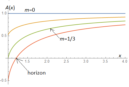
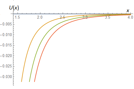
Figure 1: Example 1, the function $A(x)$ (left panel) and the potential $U(\phi(x))$ (right panel) for the Einstein-frame solution (59), (79)–(81), $m=1/6,1/3,1/2$ (upside down; at $m=0$ we have $A\equiv 1$ and $U\equiv 0$). At $x=1$, there is a naked singularity for $m\leq 1/3$ and a singularity beyond a horizon (at which $A(x)=0$) for $m>1/3$.

Let us try to use a known analytic scalar-vacuum solution of GR with a minimally coupled scalar field [44] and the scheme outlined above to obtain a solution of GHT.

If we specify the function $r(x)$, we directly find $A(x)$ from (66), so that the metric is known completely, then (60) yields $U(x)$, and it remains to find the scalar fields using (27) and (65). If, as before, we suppose $U=U({\bar{\phi}})$, the field ${\bar{\phi}}$ can be found from the first-order equation (73).

Following [44], let us choose a particular dependence $r(x)$,

$$r(x)=\sqrt{x^{2}-a^{2}},$$ (79)

and put $a=1$ as an arbitrary length scale. The inequality $r^{\prime\prime}/r=-(x^{2}-1)^{-2}<0$ confirms the canonical nature of our set of scalar fields (see Eq. (62)). Then, from (66) and (60) we find the metric function $A(x)$ and the potential [44] under the assumption that the metric is asymptotically flat, whence $A\to 1$, as $x\to\infty$:

$${}A(x)=1-3mx+\frac{3}{2}m(x^{2}-1)\log\frac{x+1}{x-1},$$ (80)

$${}U(x)=\frac{3m}{2(x^{2}\!-\!1)}\bigg{[}6x-(3x^{2}\!-\!1)\log\frac{x+1}{x-1}\bigg{]},$$ (81)

where $m={\rm const}$ has the meaning of the Schwarzschild mass in $\mathbb{M}_{\rm E}$.

The value $x=1$ corresponds to $r=0$, which is a central naked singularity for $m\leq 1/3$ and a singularity beyond an event horizon for $m>1/3$, see Fig. 1. The potential $U$ rapidly ($U\sim x^{-5}$) decays at large $x$, and $U\to-\infty$ as $x\to 1$. It is everywhere negative, so the existence of a horizon does not contradict the known no-hair theorems [43].

Assuming, as suggested above, $U=U({\bar{\phi}})$, we obtain Eq. (73) in the form

$${}3{\bar{\phi}}^{\prime}{}^{2}=\frac{1}{(x^{2}-1)^{2}}\bigg{[}1-\frac{\varepsilon C^{2}{\,\rm e}^{2{\bar{\phi}}}}{A^{2}(x)}\bigg{]},$$ (82)

with $A(x)$ given in (80). This equation can probably be solved only numerically. An exception is the case $C=0$ corresponding to $\psi={\rm const}$ which is of no interest for the theory under study since it leads to $\chi=\partial f/\partial P=0$ in its original formulation (2) (see (5) and (8)). Assuming $C\neq 0$, we notice that a change of its value is equivalent to adding a constant to ${\bar{\phi}}(x)$, which does not affect the qualitative behavior of ${\,\rm e}^{\bar{\phi}}$, and we can safely put $C=1$.

Next, Eq. (82) may be considered with both $\varepsilon=1$ (then both scalars ${\bar{\phi}}$ and $\psi$ are canonical) and $\varepsilon=-1$ (then $\psi$ is phantom but ${\bar{\phi}}$ is dominant at all $x$). Also, different solutions to Eq. (82) correspond to different signs of ${\bar{\phi}}^{\prime}$, hence there can be as many as four different solutions with the same boundary value of ${\bar{\phi}}$ specified at some fixed value of $x$.

Which kind of solutions for ${\bar{\phi}}(x)$ can be expected?

As $x\to\infty$, Eq. (82) takes the approximate form $3x^{4}{\bar{\phi}}^{\prime}{}^{2}=1-\varepsilon{\,\rm e}^{2{\bar{\phi}}}$. This equation is easily solved by substituting $x=1/\xi$, and the solution can be written as

$${}{\,\rm e}^{-2{\bar{\phi}}}\Big{|}_{\varepsilon=1}=\cosh^{2}\bigg{(}C_{1}\pm\frac{1}{\sqrt{3}x}\bigg{)},$$

$${}{\,\rm e}^{-2{\bar{\phi}}}\Big{|}_{\varepsilon=-1}=\sinh^{2}\bigg{(}C_{1}\pm\frac{1}{\sqrt{3}x}\bigg{)},$$ (83)

with $C_{1}={\rm const}$, so that ${\,\rm e}^{-2{\bar{\phi}}}$ has a finite limit at large $x$ with any $C_{1}$ if $\varepsilon=1$ and $C_{1}\neq 0$ if $\varepsilon=-1$. It confirms the general observation of Sec. 4.2.

For $m\leq 1/3$, an analysis of Eq. (82) shows that its solutions near the singularity $x=1$ either tend to a finite value or (if $m=1/3$) lead to ${\,\rm e}^{-2{\bar{\phi}}}\to\infty$, so that the singularity in $\mathbb{M}_{\rm E}$ maps according to (8) to a singularity in $\mathbb{M}_{\rm J}$.

For $m>1/3$ we arrive at a horizon with mode (iv) of the solution behavior.

In addition, for some solutions of (82), as follows from our general consideration, we can expect modes (ii) and (vii).

These inferences are confirmed by solving Eq. (73) numerically, some special solutions are plotted in Figs. 1–3, where particular asymptotic values of ${\bar{\phi}}$ as $x\to\infty$ are chosen for convenience, with no effect on the qualitative behavior of the solution.

From Fig. 2 it follows that with $\varepsilon=+1$ at $m<1/3$ we have either ${\,\rm e}^{-2{\bar{\phi}}}\to\infty$, as predicted, or we come across a monotonicity loss (mode (vii)). At $m\geq 1/3$ only mode (vii) is present.

If $\varepsilon=-1$ (Fig. 3), in the case of growing ${\bar{\phi}}$ (left panel), we obtain a finite limit of ${\bar{\phi}}$ at $m\leq 1/3$ (so that the singularity in $\mathbb{M}_{\rm E}$ is preserved in $\mathbb{M}_{\rm J}$) and mode (iv), corresponding to a horizon, at $m>1/3$. In the case of falling ${\bar{\phi}}$, hence growing ${\,\rm e}^{-2{\bar{\phi}}}$, the left ends of all curves correspond to mode (ii).

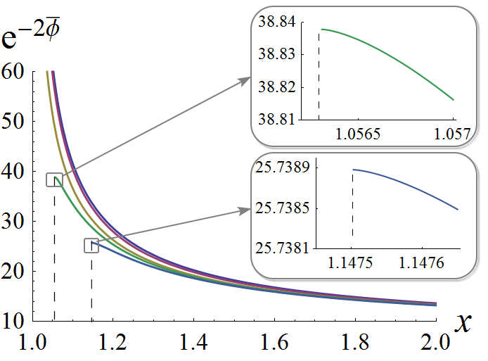
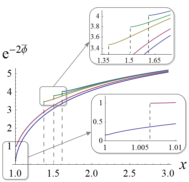
Figure 2: Example 1, the function ${\,\rm e}^{-2\bar{\phi}}$ (the conformal factor at a transition to the Jordan frame) for two branches of the solution to Eq. (73) with $\varepsilon=+1$ corresponding to ${\bar{\phi}}^{\prime}>0$ (left panel, upside-down: $m=-0.5,0,0.28,1/3,0.37$), and ${\bar{\phi}}^{\prime}<0$ (right panel, bottom-up: $m=-0.5,0,0.28,1/3,0.37$). The asymptotic value is ${\bar{\phi}}(\infty)=-1$. The insets show more clearly the behavior of some curves near their termination.

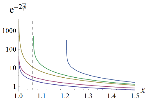
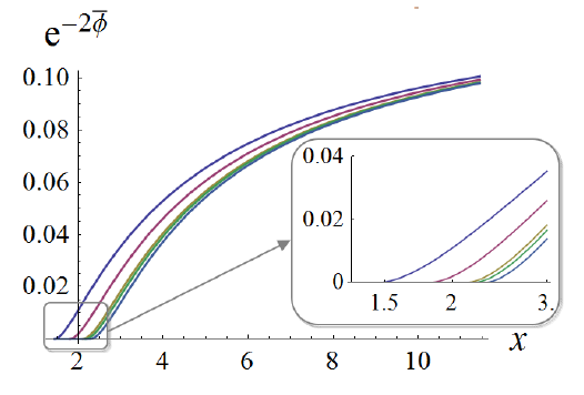
Figure 3: Example 1, the function ${\,\rm e}^{-2\bar{\phi}}$ for two branches of solution to Eq. (73) with $\varepsilon=-1$ corresponding to ${\bar{\phi}}^{\prime}>0$ (left panel, bottom-up: $m=-0.5,0,1/3,0.4,0.5$), and ${\bar{\phi}}^{\prime}<0$ (right panel, upside-down: $m=-0.5,0,1/3,0.4,0.5$). The asymptotic value is ${\bar{\phi}}(\infty)=1$.

Example 2: A solution with phantom behavior.

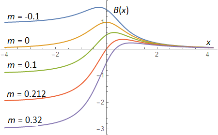
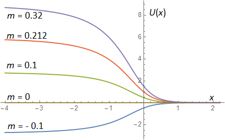
Figure 4: Example 2, the function $B(x)=A(x)/r^{2}(x)$ (left panel) and the potential $U(\phi(x))$ (right panel) for the Einstein-frame solution (59), (84)–(86), $m=-0.1,0,0.1,0.212,0.32$ (bottom-up for $B(x)$, upside down for $U(x)$. As $x\to-\infty$, the metric is asymptotically de Sitter if $m>0$ and AdS if $m<0$. At $m\approx 0.212$, the horizon occurs at $x=0$ and coincides with the minimum of $r(x)$.

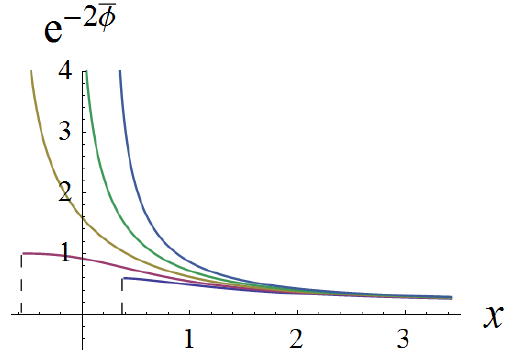
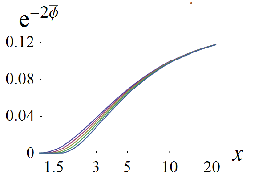
Figure 5: Example 2, the function ${\,\rm e}^{-2\bar{\phi}}$ for two branches of the solution to Eq. (73) corresponding to ${\bar{\phi}}^{\prime}>0$ (left panel, bottom-up: $m=-0.1,0,0.1,0.2,0.3$) and ${\bar{\phi}}^{\prime}<0$ (right panel, upside-down: $m=-0.1,0,0.1,0.2,0.3$). The asymptotic value is ${\bar{\phi}}(\infty)=1$.

In our second example let us assume, following [45],

$$r(x)=\sqrt{x^{2}+a^{2}},$$ (84)

and again put $a=1$ as an arbitrary length scale. The inequality $r^{\prime\prime}/r=(x^{2}+1)^{-2}>0$ confirms the phantom nature of our set of scalar fields, so that $\varepsilon=-1$. Then, assuming that the metric is asymptotically flat as $x\to\infty$, we find from (66) and (60) the metric function $A(x)$ and the potential $U(x)$ as [45] as

$${}A(x)=1+3mx-3m(x^{2}+1)\mathop{\rm arccot}\nolimits x,$$ (85)

$${}U(x)=\frac{3m}{(x^{2}+1)}\big{[}-3x+(3x^{2}+1)\mathop{\rm arccot}\nolimits x\big{]}.$$ (86)

In this solution, $x\in{\mathbb{R}}$, and $m={\rm const}$ has the meaning of the Schwarzschild mass in $\mathbb{M}_{\rm E}$. The behavior of the solution as $x\to-\infty$ depends on the sign of $m$:

• $m<0:$  $A\sim x^{2},\ U\to{\rm const}<0$ — the solution describes a wormhole with an AdS limit at the “far end”.

• $m=0:$   $A\to 1,\ U\equiv 0$ — it is the simplest (Ellis) twice asymptotically flat wormhole with zero mass [28, 30] ($A\equiv 1$, $U\equiv 0$).

• $m>0:$  $A\sim-x^{2},\ U\to{\rm const}>0$ — we obtain a regular black hole with a de Sitter expansion far beyond the horizon instead of a singularity (a “black universe” [45, 46]).

The behavior of $B(x)\equiv r^{2}(x)A(x)$ and $U(x)$ is shown in Fig. 5.

Assuming, as before, $U=U({\bar{\phi}})$, we obtain Eq. (73) in the form

$${}3{\bar{\phi}}^{\prime}{}^{2}=\frac{1}{(x^{2}+1)^{2}}\bigg{[}\frac{C^{2}{\,\rm e}^{2{\bar{\phi}}}}{A^{2}(x)}-1\bigg{]},$$ (87)

with $A(x)$ given in (85). We notice that it is necessary to put $C\neq 0$, since at $C=0$ Eq. (87) has no solution. With $C\neq 0$, as in Example 1, we put $C=1$ without loss of generality.

As $x\to\infty$, Eq. (87) takes the approximate form $3x^{4}{\bar{\phi}}^{\prime}{}^{2}={\,\rm e}^{2{\bar{\phi}}}-1$. This equation is easily solved by substituting $x=1/\xi$, and the solution can be written as

$${\,\rm e}^{-2{\bar{\phi}}}=\cos^{2}\Big{(}C_{2}\pm\frac{1}{\sqrt{3}x}\Big{)},\qquad C_{2}={\rm const},$$ (88)

so that ${\,\rm e}^{-2{\bar{\phi}}}$ has a finite limit at large $x$, unless $C_{2}=(n+{{\textstyle\frac{1}{2}}})\pi$ with integer $n$. It confirms the general observation of Sec. 4.2.

The other end of the $x$ range depends on the sign of $m$. The case $m=0$ returns us to the already considered systems with zero potential, so let us suppose $m\neq 0$.

If $m>0$, there is a horizon in $\mathbb{M}_{\rm E}$ at some finite $x=x_{h}$, where we find the behavior denoted as (iv).

If $m<0$, the other end is at $x\to-\infty$, where $A(x)\sim x^{2}$, and we can expect modes (vi-a) and (vi-b).

In addition, with any $m$, we cannot exclude the emergence of modes (ii) and (vii). The particular kind of solution should depend on the initial condition for ${\bar{\phi}}$, specified at some value of $x$.

Solving Eq. (87) numerically, we find for ${\bar{\phi}}^{\prime}>0$ (Fig. 5, left) two modes, (vii) if $m\leq 0$ and (iv) if $m>0$, the latter corresponding to a horizon. For ${\bar{\phi}}^{\prime}<0$ (Fig. 5, right) we find mode (ii) at all values of $m$.

Example 3: A trapped-ghost solution.

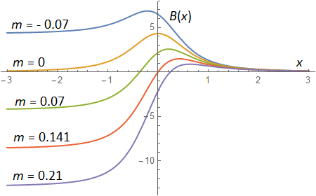
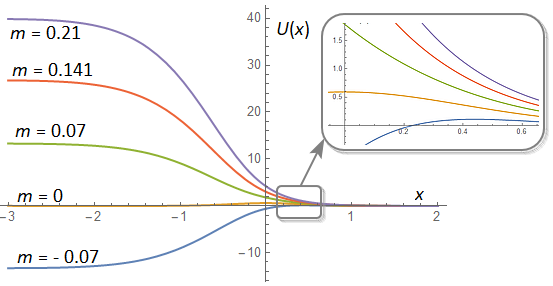
Figure 6: Example 3, the function $B(x)=A(x)/r^{2}(x)$ (left panel) and the potential $U(\phi(x))$ (right panel) for the Einstein-frame solution (59), (89)–(4.3), $m=-0.07,0,0.07,0.141,0.21$ (bottom-up for $B(x)$, upside down for $U(x)$). The right panel shows a detailed behavior of $U$ at small $x$. As $x\to-\infty$, the metric is asymptotically de Sitter if $m>0$ and AdS if $m<0$. At $m\approx 0.141$, the horizon occurs at $x=0$ and coincides with the minimum of $r(x)$.

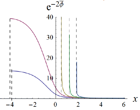
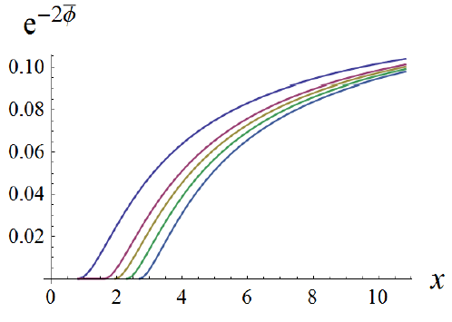
Figure 7: Example 3, the function ${\,\rm e}^{-2{\bar{\phi}}}$ for two branches of solution to Eq. (73) corresponding to ${\bar{\phi}}^{\prime}>0$ (left panel, from left to right: $m=-0.9,0,0.3,0.6,0.9$) and ${\bar{\phi}}^{\prime}<0$ (right panel, from top to bottom: $m=-0.9,0,0.3,0.6,0.9$). The asymptotic value ${\bar{\phi}}(\infty)=1$.

The following choice of $r(x)$ [32] instead of (79) or (84),

$$r(x)=a\frac{x^{2}+1}{\sqrt{x^{2}+3}},\qquad a={\rm const},$$ (89)

presents an example of a so-called trapped-ghost behavior [47] of the scalar fields since the quantity

$$\frac{r^{\prime\prime}}{r}=\frac{1}{a^{2}}\frac{15-x^{2}}{(x^{2}+3)^{2}(x^{2}+1)}$$ (90)

is positive at small $x$ (in the “strong field region”) and negative at large $x$. Meanwhile (see Eq. (62)), $r^{\prime\prime}/r>0$ is an indicator of a phantom behavior of matter in GR because $r^{\prime\prime}/r\sim-T^{t}_{t}+T^{x}_{x}=-(\rho+p_{r})>0$ in standard notations, which manifests NEC violation. With (90), we have a phantom behavior only at $x^{2}<15$.

In our case with two scalars ${\bar{\phi}}$ and $\psi$, the first one is always canonical, and the ansatz (84) means that the second, phantom field $\psi$ is dominant at small $x$ and subdominant at large $x$.

Let us put, as before, $a=1$ and require asymptotic flatness as $x\to\infty$. Then, with the ansatz (89), the metric function $A(x)$ and the potential $U(x)$ have the form [32]

$${}A(x)=\frac{(x^{2}+1)^{2}}{x^{2}+3}\biggl{[}\frac{39m}{2}\Big{(}\arctan x-\frac{\pi}{2}\Big{)}$$

$${}+\frac{26+\!24x^{2}\!+\!6x^{4}+3mx(69+100x^{2}+39x^{4})}{6(1+x^{2})^{3}}\bigg{]},$$

(91)

$${}U(x)=\frac{1}{12(1+\!x^{2})^{2}(3+\!x^{2})^{3}}\Big{[}32(-6+x^{2}+3x^{4})$$

$${}+6mx(2655+\!6930x^{2}\!+\!5420x^{4}\!+\!1326x^{6}\!+\!117x^{8})$$

$${}+117m(1+x^{2})^{2}(15+89x^{2}+29x^{4}+3x^{6})$$

$${}\hskip 72.26999pt\times(-\pi+2\arctan x)\Big{]}.$$ (92)

Despite different analytical expressions, the qualitative features of $A(x)$ and $U(x)$ are here almost the same as in Example 2, see Fig. 7. The main difference is that at $m=0$ we now have $A(x)\neq{\rm const}$ and $U\not\equiv 0$, so this case (a twice asymptotically flat wormhole) is not covered by the description in Section 3.

Accordingly, the behavior of the corresponding solutions to Eq. (73) in this case should contain the same modes as in Example 2, and, in addition, mode (v) for $m=0$.

These inferences are confirmed by solving Eq. (73) numerically, as demonstrated by Fig. 7.

5 Concluding remarks

We have considered exact analytical static, spherically symmetric solutions of GHT (generalized HMPG) without matter, making use its scalar-tensor representation with two effective scalar fields [17], with zero potential $V(\chi,\xi)=W(\phi,\xi)$ and some special cases of nonzero potentials. The results are compared with their counterparts in the simpler version of the theory, “genuine” HMPG [4], obtained previously [13, 14]. As before, we use the Einstein conformal frame $\mathbb{M}_{\rm E}$ to solve the equations and then a transition back to the original Jordan frame $\mathbb{M}_{\rm J}$ in which the theory is formulated and interpreted.

In the case of zero potential, $V\equiv 0$, the set of resulting space-time metrics includes all metrics discussed in [13, 14] for $V\equiv 0$, plus two new families (Branches 2 and 3) whose emergence is directly related with a more complex scalar field configuration. While in HMPG the whole set of solutions splits into two sectors, the canonical and phantom ones according to the nature of the single scalar field, in the present case emerges a more intricate interplay between two scalars when one of them is canonical and the other phantom. One of the new families of solutions corresponds to their equilibrium, with the Schwarzschild metric in $\mathbb{M}_{\rm E}$ and its certain deformation in $\mathbb{M}_{\rm J}$.

As in HMPG, generic solutions either contain naked singularities or, in the case of a phantom behavior of the scalar field set, describe traversable wormholes. Black-hole solutions in $\mathbb{M}_{\rm J}$ emerge only due to conformal continuations [38] and form two special families with double (extreme) horizons. This feature of scalar-tensor solutions with $V=0$ could be expected due to the well-known no-hair theorems.

Some exact solutions with $V\not\equiv 0$ have been obtained under assumptions quite similar to those used in [13, 14], and the Einstein-frame metrics are the same as were known previously in [44, 45, 46]. However, the conformal factor needed to transfer the metric to $\mathbb{M}_{\rm J}$ is found only numerically, and it has turned out that even black hole solutions existing in $\mathbb{M}_{\rm E}$ become those with naked singularities in $\mathbb{M}_{\rm J}$. A new feature of GHT as compared to GMPG is the existence of solutions with trapped-ghost properties [47], but in the example considered here such a solution behaves similarly to the one with a phantom-like scalar set.

From our Examples 1–3 one might conclude that all GHT solutions with a nonzero potential contain naked singularities, since even a horizon in $\mathbb{M}_{\rm E}$ maps to a singularity in $\mathbb{M}_{\rm J}$. These are, however, only special cases under the special assumption $U=U({\bar{\phi}})$, and more general solutions are yet to be found.

In [14] some results were reported on the stability properties of HMPG solutions, but they cannot be extended to GHT even in cases where the metrics are the same, due to a more complex nature of the scalar field set. Such a stability study is a task for the near future and can be probably performed by analogy with [48, 49, 31, 50, 32] etc. Another possible continuation of the present study is its extension including electromagnetic fields, which can be done rather easily for the case $V=0$ by analogy with [28, 51] but only with the aid of numerical methods for $V\neq 0$ even if we use in $\mathbb{M}_{\rm E}$ siutable solutions known in GR [52, 53] as a basis.

Funding

This publication was supported by the RUDN University Strategic Academic Leadership Program and by RFBR Project 19-02-00346. K.B. was also funded by the Ministry of Science and Higher Education of the Russian Federation, Project “Fundamental properties of elementary particles and cosmology” N 0723-2020-0041,

References

- [1] E.J. Copeland, M. Sami and S. Tsujikawa, “Dynamics of dark energy,” Int. J. Mod. Phys. D 15, 1753 (2006); hep-th/0603057.
- [2] S. Capozziello and M. De Laurentis, “Extended Theories of Gravity,” Phys. Rep. 509, 167 (2011); arXiv: 1108.6266.
- [3] S.-i. Nojiri and S.D. Odintsov, “Introduction to modified gravity and gravitational alternative for dark energy,” Int. J. Geom. Meth. Mod. Phys. 4, 115 (2007).
- [4] T. Harko, T.S. Koivisto, F.S.N. Lobo and G.J. Olmo, “Metric-Palatini gravity unifying local constraints and late-time cosmic acceleration,” Phys. Rev. D 85, 084016 (2012); arXiv: 1110.1049.
- [5] Salvatore Capozziello, Tiberiu Harko, Francisco S.N. Lobo, and Gonzalo J. Olmo, “Hybrid modified gravity unifying local tests, galactic dynamics and late-time cosmic acceleration,” Int. J. Mod. Phys. D 22, 1342006 (2013); arXiv: 1305.3756.
- [6] S. Capozziello, T. Harko, T.S. Koivisto, F.S.N. Lobo, and G.J. Olmo, “The virial theorem and the dark matter problem in hybrid metric-Palatini gravity,” JCAP 07, 024 (2013). arXiv: 1212.5817.
- [7] S. Capozziello, T. Harko, T. S. Koivisto, F.S.N. Lobo, and G.J. Olmo, “Cosmology of hybrid metric-Palatini f(X)-gravity,” JCAP 04, 011 (2013); arXiv: 1209.2895.
- [8] S. Capozziello, T. Harko, T.S. Koivisto, F.S.N. Lobo, and G.J. Olmo, “Hybrid metric-Palatini gravity,” Universe 1, 199 (2015); arXiv: 1508.04641.
- [9] T. Harko and F.S.N. Lobo, Extensions of Gravity: Curvature-Matter Couplings and Hybrid Metric-Palatini Theory (Cambridge University Press, Cambridge, UK, 2018).
- [10] A. Borowiec, S. Capozziello, M. De Laurentis, F. S. N. Lobo, A. Paliathanasis, M. Paolella, and A. Wojnar, “Invariant solutions and Noether symmetries in Hybrid Gravity,” Phys. Rev.D 91, 023517 (2015); arXiv: 1407.4313.
- [11] Ariel Edery and Yu. Nakayama, “Palatini formulation of pure gravity yields Einstein gravity with no massless scalar,” Phys. Rev. D 99, 124018 (2019); arXiv: 1902.07876.
- [12] Bogdan Dǎnilǎ, Tiberiu Harko, Francisco S. N. Lobo, and Man Kwong Mak, “Spherically symmetric static vacuum solutions in hybrid metric-Palatini gravity,” Phys. Rev. D 99, 064028 (2019); arXiv: 1811.02742.
- [13] K.A. Bronnikov, “Spherically symmetric black holes and wormholes in hybrid metric-Palatini gravity,” Grav. Cosmol. 25, 331 (2019); arXiv: 1908.02012.
- [14] K. A. Bronnikov, S. V. Bolokhov, M. V. Skvortsova, “Hybrid metric-Palatini gravity: black holes, wormholes, singularities and instabilities,” Grav. Cosmol. 26, 212–227 (2020); arXiv: 2006.00559.
- [15] T. Harko, F.S.N. Lobo, and H.M.R. da Silva, “Cosmic stringlike objects in hybrid metric-Palatini gravity,” Phys. Rev. D 101, 124050 (2020).
- [16] K. A. Bronnikov, S. V. Bolokhov, and M. V. Skvortsova, “Hybrid metric-Palatini gravity: Regular stringlike configurations,” Universe 6, 172 (2020); arXiv: 2009.03952.
- [17] C.G. Böhmer and N. Tamanini, “Generalized hybrid metric-Palatini gravity,” Phys. Rev. D 87, 084031 (2013); arXiv:1302.2355.
- [18] João L. Rosa, Sante Carloni, José P. S. Lemos, and Francisco S. N. Lobo, “Cosmological solutions in generalized hybrid metric-Palatini gravity,” Phys. Rev. D .95, 124035 (2017); arXiv:1703.03335.
- [19] João L. Rosa, Sante Carloni, and José P. S. Lemos, “Cosmological phase space of generalized hybrid metric-Palatini theories of gravity,” Phys. Rev. D 101, 104056 (2020); arXiv: 1908.07778.
- [20] Paulo M. Sá, “Unified description of dark energy and dark matter within the generalized hybrid metric-Palatini theory of gravity,” Universe 6, 78 (2020); arXiv: 2002.09446.
- [21] Flavio Bombacigno, Fabio Moretti, and Giovanni Montani, “Scalar modes in extended hybrid metric-Palatini gravity: weak field phenomenology,” arXiv: 1907.11949.
- [22] João Luís Rosa, Francisco S.N. Lobo, and and Gonzalo J. Olmo, “Weak-field regime of the generalized hybrid metric-Palatini gravity,” arXiv: 2104.10890.
- [23] João L. Rosa, José P. S. Lemos, and Francisco S. N. Lobo, “Stability of Kerr black holes in generalized hybrid metric-Palatini gravity,” Phys. Rev. D 101, 044055 (2020); arXiv: 2003.00090.
- [24] João Luís Rosa, José P. S. Lemos, and Francisco S. N. Lobo, “Wormholes in generalized hybrid metric-Palatini gravity obeying the matter null energy condition everywhere,” Phys. Rev. D 98, 064054 (2018); arXiv: 1808.08975.
- [25] Tiberiu Harko and Francisco S.N. Lobo, “ Beyond Einstein’s General Relativity: Hybrid metric-Palatini gravity and curvature-matter couplings,” arXiv: 2007.15345.
- [26] R. Wagoner, “Scalar-tensor theory and gravitational waves,” Phys. Rev. D 1, 3209 (1970).
- [27] K.A. Bronnikov, S.V. Chervon, and S.V. Sushkov. “Wormholes supported by chiral fields,” Grav. Cosmol. 15, 3, 241–246 (2009); ArXiv: 0905.3804.
- [28] K.A. Bronnikov. “Scalar-tensor theory and scalar charge,” Acta Phys. Pol. B 4, 251 (1973).
- [29] K.A. Bronnikov and S.G. Rubin, Black Holes, Cosmology, and Extra Dimensions (World Scientific: Singapore, 2013).
- [30] H. Ellis, “Ether flow through a drainhole — a particle model in general relativity,” J. Math. Phys. 14, 104 (1973).
- [31] K.A. Bronnikov, J.C. Fabris, and A. Zhidenko, “On the stability of scalar-vacuum space-times,” Eur. Phys. J. C 71, 1791 (2011).
- [32] K.A. Bronnikov, “Scalar fields as sources for wormholes and regular black holes,” Particles 2018, 1, 5 (2018); arXiv: 1802.00098.
- [33] I.Z. Fisher, “Scalar mesostatic field with regard for gravitational effects,” Zh. Eksp. Teor. Fiz. 18, 636 (1948); gr-qc/9911008.
- [34] P. Jordan, Schwerkraft und Weltall (Vieweg, Braunschweig, 1955).
- [35] N.M. Bocharova, K.A. Bronnikov, and V.N. Melnikov. “On an exact solution of the Einstein-scalar field equations,” Vestnik Mosk Univ., Fiz., Astron. No. 6, 706 (1970).
- [36] J.D. Bekenstein, “Black holes with scalar charge,” Ann. Phys. (NY) 82, 535 (1974).
- [37] K.A. Bronnikov, “Scalar vacuum structure in general relativity and alternative theories. Conformal continuations,” Acta Phys. Polon. B 32, 3571 (2001); gr-qc/0110125.
- [38] K.A. Bronnikov, “Scalar-tensor gravity and conformal continuations,” J. Math. Phys. 43, 6096 (2002); gr-qc/0204001.
- [39] K.A. Bronnikov and A.A. Starobinsky, “No realistic wormholes from ghost-free scalar-tensor phantom dark energy,” Pis’ma v ZhETF 85, 3–8 (2007); JETP Lett. 85, 1–5 (2007); gr-qc/0612032.
- [40] O. Bergmann and R. Leipnik, “Space-time structure of a static spherically symmetric scalar field,” Phys. Rev. 107, 1157 (1957).
- [41] Carlos A. R. Herdeiro and Eugen Radu, “Asymptotically flat black holes with scalar hair: a review,” Int. J. Mod. Phys, D 24, 1542014 (2015); arXiv: 1504.08209.
- [42] K.A. Bronnikov, “Spherically symmetric false vacuum: no-go theorems and global structure,” Phys. Rev. D 64, 064013 (2001); gr-qc/0104092.
- [43] S. A. Adler and R. P. Pearson, “”No-hair” theorems for the Abelian Higgs and Goldstone models,” Phys. Rev. D 18, 2798 (1978).
- [44] K.A. Bronnikov and G.N. Shikin, “Spherically symmetric scalar vacuum: no-go theorems, black holes and solitons,” Grav. Cosmol. 8, 107 (2002); gr-qc/0109027.
- [45] K.A. Bronnikov and J.C. Fabris, “Regular phantom black holes,” Phys. Rev. Lett. 96, 251101 (2006); gr-qc/0511109.
- [46] K.A. Bronnikov, V.N. Melnikov and H. Dehnen, “Regular black holes and black universes,” Gen. Rel. Grav. 39, 973–987 (2007); gr-qc/0611022.
- [47] K.A. Bronnikov and S.V. Sushkov, “Trapped ghosts: a new class of wormholes,” Class. Quantum Grav. 27, 095022 (2010); arXiv: 1001.3511.
- [48] K.A. Bronnikov and A.V. Khodunov. “Scalar field and gravitational instability,” Gen. Rel. Grav.11, 13 (1979).
- [49] J.A. Gonzalez, F.S. Guzman, and O. Sarbach, “Instability of wormholes supported by a ghost scalar field. I. Linear stability analysis,” Class. Quantum Grav. 26, 015010 (2009); arXiv: 0806.0608.
- [50] K.A. Bronnikov, R.A. Konoplya, and A. Zhidenko, “Instabilities of wormholes and regular black holes supported by a phantom scalar field,” Phys. Rev. D 86, 024028 (2012); arXiv: 1205.2224.
- [51] K.A. Bronnikov, C.P. Constantinidis, R.L. Evangelista, and J.C. Fabris, “Electrically charged cold black holes in scalar-tensor theories,” Int. J. Mod. Phys. D 8, 481 (1999); gr-qc/9902050
- [52] S.V. Bolokhov, K.A. Bronnikov, and M.V. Skvortsova, “Magnetic black universes and wormholes with a phantom scalar,” Class. Quantum Grav. 29, 245006 (2012); arXiv: 1208.4619.
- [53] K.A. Bronnikov and P.A. Korolyov, “Magnetic wormholes and black universes with invisible ghosts,” Grav. Cosmol. 21, 157 (2015); arXiv: 1503.02956.