Evidence of a Tidal-disruption Event in GSN 069 from the Abnormal Carbon and Nitrogen Abundance Ratio

Abstract

GSN 069 is an ultra-soft X-ray active galactic nucleus that previously exhibited a huge X-ray outburst and a subsequent long-term decay. It has recently presented X-ray quasi-periodic eruptions (QPEs). We report the detection of strong nitrogen lines but weak or undetectable carbon lines in its far ultraviolet spectrum. With a detailed photoionization model, we use the C iv/N iv] ratio and other ratios between nitrogen lines to constrain the [C/N] abundance of GSN 069 to be from $-3.33$ to $-1.91$. We argue that a partially disrupted red giant star can naturally explain the abnormal C/N abundance in the UV spectrum, while the surviving core orbiting the black hole might produce the QPEs.

1 Introduction

GSN 069 is an optically identified very low-mass bona-fide type 2 active galactic nuclei (AGN) with ultra-soft X-ray emission (Miniutti et al., 2013). It is the first case that presents X-ray quasi-periodic eruptions (QPEs) (Miniutti et al., 2019). The X-ray emission of GSN 069 was first detected in 2010 and implied an outburst with a factor of more than 240 increase in flux compared to the quiescence state (Miniutti et al., 2013). It has since shown a long-term decay (Shu et al., 2018).

These observed properties were interpreted in several different scenarios. One possible interpretation links the outburst in 2010 to the AGN re-activation after a period of quiescence. In this case, the QPEs are driven by an accretion-flow instability, reminiscent of the heartbeat variability of black hole X-ray binaries (Belloni et al., 1997; Altamirano et al., 2011; Miniutti et al., 2019). Another plausible scenario is that GSN 069 could experience a long-lived tidal-disruption event (TDE), manifesting a slow long decay of X-ray flux and spectral evolution (Shu et al., 2018). Alternatively, King (2020) suggested a stellar-mass white dwarf in a highly eccentric orbit about a massive black hole could reproduce the QPEs of GSN 069, while Ingram et al. (2021) proposed a self-lensing binary massive black hole interpretation. The last two works did not explain the long-term X-ray variations. Although similar X-ray QPEs have been detected in three more galaxies (Sun et al., 2013; Giustini et al., 2020; Arcodia et al., 2021), including two previously inactive ones, their origin remains a puzzle.

Previous studies suggested that TDEs display a unique ultraviolet (UV) emission-line spectrum, characterized by strong nitrogen lines and weak carbon lines, distinct from those of AGNs (Cenko et al., 2016; Yang et al., 2017; Brown et al., 2018). This is intriguing because, in normal AGNs, the carbon emission lines like C iii] or C iv are usually much stronger than nitrogen lines (Vanden Berk et al., 2001), and even in rare nitrogen-rich (N-rich) AGNs there are significant carbon lines (e.g., the most N-rich AGN Q0353-383, Baldwin et al., 2003). Enhancement in metallicity due to the stellar population has challenges in explaining the AGNs’ N-rich phenomenon. TDEs can provide a more natural explanation because of supplying a significant mass of N-rich/carbon-poor material (Cenko et al., 2016; Kochanek, 2016). Interestingly, examining the UV spectra of TDEs, Yang et al. (2017) suggested the C iii]$\lambda 1908$/N iii]$\lambda 1750$ ratio is a good indicator of N/C abundance and derived abundance ratios for three TDEs which indicate nitrogen-enhanced core material of a disrupted star. Moreover, adopting this N/C abundance indicator, Liu et al. (2018) reported a candidate TDE in N-rich quasars (Jiang et al., 2008; Batra & Baldwin, 2014) via abundance ratio variability.

Inspired by these findings, we analyze the UV spectrum of GSN 069 to explore the possible clues to the question whether QPEs are directly associated with accretion-flow instabilities or due to extrinsic phenomena (e.g., such as a TDE or the presence of an orbiting body). Strikingly, we find that the nitrogen lines are anomalously strong, while the carbon lines (e.g., C iii] and C iv) are weak or nearly absent. We use the photoionization model to investigate the formation of nitrogen lines in GSN 069’s UV spectrum, and explore the applicability of using the C iv/N iv] line ratio as well as the ratios between different nitrogen lines to constrain the C/N abundance ratio.

2 UV Spectral decomposition

GSN 069 was observed twice spectroscopically in the far-UV (FUV) and near-UV (NUV) by the Space Telescope Imaging Spectrograph on board the Hubble Space Telescope, using the Multi-Anode Microchannel Array detector with the G140L and G230L gratings (Program ID: 13815 and 15442, PI: Miniutti 2019). The first observation was performed in 2014 December and the second was in 2018 December. In each epoch, there were two 49 minute FUV and one 39 minute NUV exposures. We downloaded the pipeline-calibrated one-dimensional spectra from the Hubble Legacy Archive . After checking that there was no significant variability between the two epochs, the FUV and NUV spectra were signal-to-noise ratio (S/N) weighted and combined to a single spectrum covering the full UV range from 1130$\sim$3100 Å. Then, we dereddened the Milky Way absorption according to the dust map provided by Schlegel et al. (1998).

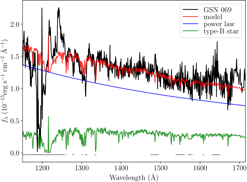
Figure 1: Spectral decomposition of GSN 069. We show the UV spectrum of GSN 069 in black, and the best fitting model in red. The blue line represents the decomposed continuum, while the green spectrum represents the type-B-star template. The gray lines at the bottom represent the masked region when performing decomposition.

As mentioned by Miniutti et al. (2019), the UV spectrum of GSN 069 resembles that of the main-sequence star (e.g., type-B star, see Extended Data Fig.2a of Miniutti et al. 2019), indicating that it is likely contaminated by a relatively young stellar nuclear cluster. To remove the starlight contamination, we use intermediate early-type stars’ co-added spectra (e.g., type-B0, -B3 and -B6 stars) from the Hubble Spectroscopic Legacy Archive (HSLA) to build a template stellar spectrum. We require that the spectra should have high S/N and cover the emission lines that we are interested in (e.g., N v, N iv], C iv, N iii] and C iii]). Also, no grating gaps should be present around these main emission lines. Only three stars satisfy our requirement, namely NGC1818-D1, EC05438-4741 and EC10500-1358, which are classified as B0-2 V-IV, B3-5 V-IV and B6-9.5 V-IV star, respectively (we mark them as T1, T2 and T3). However, only FUV data are available on the HSLA, so all the three stars’ spectra did not cover the C iii]$\lambda$1909 Å. After resampling these spectra to match the resolution of GSN 069, their median S/N turned to 156.1, 78.7 and 101.1, respectively. We normalized the three spectra using the median flux between 1445 and 1455 Å to get the templates.

Before the fitting process, we masked out regions of the prominent emission lines of GSN 069, strong Galactic absorption lines as well as geocoronal lines (see the bottom gray line in Figure 1). By adding a power-law continuum component to the mixed type B-star templates, the model can be written as,

$$f=A\times(\lambda/1000)^{\alpha}+a\times T_{1}+b\times T_{2}+c\times T_{3}$$ (1)

where (A,$\alpha$,a,b,c)=(1.71$\pm$0.04, $-$1.57$\pm$0.05, 0.04$\pm$0.02, 0, 0.29$\pm$0.02).

Thus, the continuum and the B-star components can be removed from the original spectrum to get the emission lines of GSN 069 (see Figure 2). We use one Gaussian to model the single line (N iv] and He ii) and two Gaussian’s to model the doublets (N v, N iv] and C iv). Considering the N iv]  has the best profiles and S/N, we firstly fit the N iv]. With the best fitted N iv], the profiles of C iv, He ii and N iii] are assumed to be the same as N iv]. In order to estimate the uncertainties, we generate 100 mock spectra by adding Gaussian noise to the spectrum using the uncertainty of input data. By repeating the fit procedure, the standard deviation of the distributions of best fit is taken as the uncertainty for each spectral quantity.

The fitted line flux of N v, N iv], C iv, He ii, N iii] are 5.16$\pm$0.19, 1.24$\pm$0.19, 0.50$\pm$0.19, 1.65$\pm$0.27 and 0.91$\pm$0.31 (in unit of $10^{-15}\rm erg/s/cm^{2}$), respectively. Although our B-star templates do not cover C iii], we examined the theoretical stellar spectra of B stars (Castelli & Kurucz, 2003; Castelli, 2005) and found no strong absorption around the C iii] emission lines. We fit a Gaussian and a local continuum to spectrum in C iii] window. The line is completely not detected.

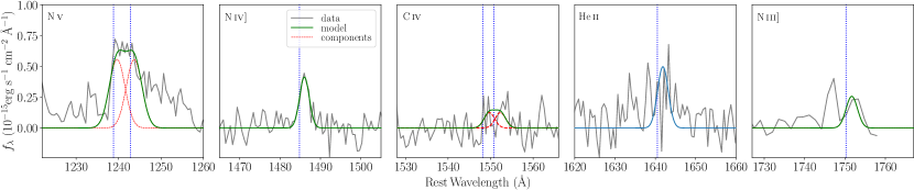
Figure 2: Emission lines of GSN 069. In each panel, we show the starlight and continuum subtracted spectrum in gray, and we use the vertical dotted lines to mark the wavelength of the emission lines. The blue and red lines represent the emission line models and components, respectively.

3 Constraint on the C/N ratio

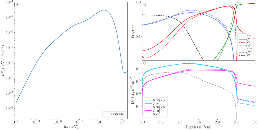
Figure 3: Panel (A) presents the SED of GSN 069. Panel (B) and (C) present ionization fractions and depth-weighted line emissivities against spatial depth into a cloud having $U=-0.2$, $n_{\rm H}=10^{10}\rm cm^{-3}$, solar abundances, and an incident SED of GSN 069. The dashed curves represent nitrogen and the solid curves represent carbon.

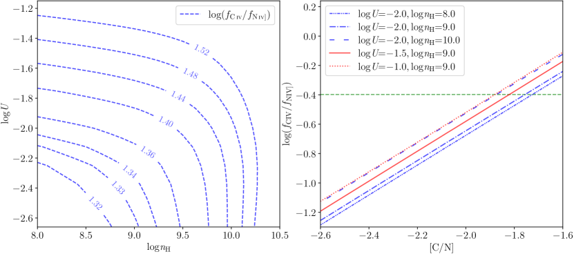
Figure 4: Left panel: contour plots for the logarithmic line ratio of C iv/N iv] in the $U\sbond n_{\rm H}$ plane at solar metallicity. Right panel: theoretical logarithmic line ratios of C iv/N iv] as a function of [C/N] in different $U$ and $n_{\rm H}$. The horizontal green dashed line marks the observed C iv/N iv]  ratio of GSN 069.

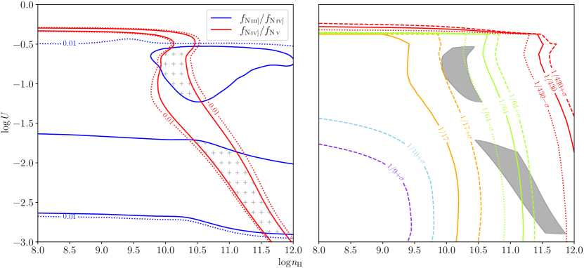
Figure 5: Left panel: contour plots for the allowed region in $U\sbond n_{\rm H}$ plane defined by the $f_{\rm N\,\textsc{iii]}}/f_{\rm N\,\textsc{iv]}}$ (blue) and $f_{\rm N\,\textsc{iv]}}/f_{\rm N\,\textsc{v}}$ (red), respectively. The solid and dotted lines represent the 95% and 99% confidence level of line ratios, respectively. The gray cross symbols roughly mark the enclosed area jointly defined by the $f_{\rm N\,\textsc{iii]}}/f_{\rm N\,\textsc{iv]}}$ and $f_{\rm N\,\textsc{iv]}}/f_{\rm N\,\textsc{v}}$ (taking the 95% confidence level, respectively). Right panel: the gray shadow area is the same allowed region jointly defined by the $f_{\rm N\,\textsc{iii]}}/f_{\rm N\,\textsc{iv]}}$ and $f_{\rm N\,\textsc{iv]}}/f_{\rm N\,\textsc{v}}$ as marked in the left panel. The solid line contours are $f_{\rm C\,\textsc{iv}}/f_{\rm N\,\textsc{iv]}}$ at the observed value for different carbon abundance, while the dashed and dotted lines represent the corresponding 1$\sigma$ upper limit and 1$\sigma$ lower limit of the observed value (marked with the additional label $+1\sigma$ and $-1\sigma$), respectively. From lower left to upper right, the carbon abundance decreasing from $Z_{C,\sun}$/9 to $Z_{C,\sun}$/430. The models with 1/17 to 1/430 solar carbon abundances intersect the allowable shadowed gray region.

Our goal is to constrain C/N ratio of GSN 069 from its observed UV line ratios. Previous works have used the ratios of nitrogen emission lines to various collisional/recombination lines of other elements to derive the metal abundance in the broad line region (BLR) of quasars based on the chemical enrichment that nitrogen is produced by a secondary process (Hamann & Ferland 1993, 1999; Hamann et al. 2002; Batra & Baldwin 2014). Yang et al. (2017) showed that C iii]/N iii] ratio is a good indicator of [N/C] abundance ratio that is insensitive to the shape of the ionizing continuum or the physical parameters of the emission line region over wide parameter ranges. Accordingly, they set a lower limit on the N/C ratio for three TDEs. Because C iii] is not detected and N iii] is only marginally detected in GSN 069, it is not possible to employ the same method. However, N iv] and N v are prominent in GSN 069, so we will use the C iv/N iv] and ratios of between different nitrogen lines to constrain the C/N abundance ratio and the physical conditions of the line emission region. Although a large number of grid models already exist in the literature for the conditions of BLR in quasars (Korista et al., 1997), more precise modeling requires a good match in the input ionizing continuum to that of GSN 069 and the specific chemical abundance. Thus we run a set of photoionization models using CLOUDY 17.02 (Ferland et al., 2017) by taking these into consideration.

We adopt an SED derived by fitting a disk-corona model to the observed data from optical UV to X-ray (Miniutti et al., 2013), which is shown in the left panel of Figure 3. Although it is still unclear whether there are cold gas clouds on a BLR scale in the nuclei of low-luminosity AGNs or quiescent galaxies, some theoretical and observational works suggest that BLR disappears when the Eddington ratio of an AGN is below 0.001 (e.g., Elitzur & Ho 2009). The abnormal [N/C] in two of three TDEs analyzed by Yang et al. (2017), suggests that they are unlikely normal ISM, even considering the high metallicity in galactic nuclei (Nagao et al., 2006). As for the TDE, the disrupted debris, either in outflow or accretion disk, is predicted to be photoionized and produce optical emission lines (Roos 1992, Bogdanović et al. 2004, Strubbe & Quataert 2009). The gaseous debris of a star can be high density and may well have an unusual chemical composition (Cenko et al., 2016; Kochanek, 2016). In analog with an analysis of BLR of AGNs (Peterson 1997, p. 73), only $\sim 10^{-3}\rm M_{\sun}$ line emitting gas is required to produce the emission lines. So in the context of the tidal-disruption model, the line emitting gas is assumed to come from the interior of a star that is polluted with nuclear fusion production.

For main-sequence stars, which account for the majority of observed TDEs, most carbon in the center of the star is converted into nitrogen in a relatively short time in the CNO cycle. In equilibrium, the C/N ratio is a function of temperature. We set the overall abundance to solar values given by Grevesse et al. (2010), but the allow carbon and nitrogen ratio to vary while the sum of carbon and nitrogen is maintained to the solar value according to the CN cycle. Then a set of plane-parallel slab models with constant density and ionization parameter are computed. The logarithm of gas density ($n_{\rm H}$) in cm^-3 runs from 8 to 12, and the logarithm of ionization parameters (${\rm U}=\Phi/4\pi r^{2}n_{\rm H}c$, where $\Phi$ is the flux of ionizing photons and $c$ is the speed of light) from -3 to 0. Both the $n_{\rm H}$ and $U$ are run with an initial step of 0.25 dex to estimate the range of parameters and a fine grid of models with a step of 0.125 dex around plausible parameter regimes are computed later to determine more precisely the physical conditions and the upper limit of carbon abundance.

In the panel (B) of Figure 3, we present the ionization structure of a cloud having $\rm log\emph{U}=-0.2$, $n_{\rm H}=10^{10}\rm cm^{-3}$, solar abundances, and an incident SED of GSN 069, while the depth-weighted line emissivities against spatial depth are shown in the panel (C). The emission regions of C iv and N iv] significantly overlap as well as that of C iii] and N iii], indicating these pairs are also good abundance indicators (similar plots were also presented by Hamann et al. 2002). We firstly examine the dependences of the line ratio of C iv/N iv] (herein after, $f_{\rm C\,\textsc{iv}}/f_{\rm N\,\textsc{iv]}}$) upon the $U$, $n_{\rm H}$ and [C/N] abundance. In the left panel of Figure 4, we plot the contours of logarithmic $f_{\rm C\,\textsc{iv}}/f_{\rm N\,\textsc{iv]}}$ in the $U\sbond n_{\rm H}$ plane at solar abundance as an example. At the given [C/N] abundance and $U$, when the density is lower than the critical density of N iv] ($n_{c}\sim 10^{10}\rm cm^{-3}$), the $f_{\rm C\,\textsc{iv}}/f_{\rm N\,\textsc{iv]}}$ is not sensitive to the density (e.g., when $n_{\rm H}$ varied $\sim$1 dex, the ratio just changes $\sim$0.04 dex). However, while the $n_{\rm H}$ is approaching the critical density, the contours drop significantly due to collisional de-excitation of N iv] is overwhelming. The $f_{\rm C\,\textsc{iv}}/f_{\rm N\,\textsc{iv]}}$ also has a weak dependence with $U$. For example, by fixing the $n_{\rm H}=8.0$, when the $\rm log\emph{U}$ changes from $-2.2$ to $-1.2$ (1 dex), the ratio just changes $\sim$0.2 dex. This weak dependence on density or ionization is much clearer in the right panel of Figure 4, in which we plot theoretical logarithmic $f_{\rm C\,\textsc{iv}}/f_{\rm N\,\textsc{iv]}}$ as a function of [C/N] in different $\rm log\emph{U}$ and $\rm log\emph{n}_{\rm H}$. We can see that the $f_{\rm C\,\textsc{iv}}/f_{\rm N\,\textsc{iv]}}$ significantly depends on the [C/N]. A similar plot is also presented by Yang et al. (2017) who used the C iii]/N iii] ratio against [C/N] to constrain the carbon abundance of three TDEs. Thus, following Yang et al. (2017), we can also estimate the carbon abundance of GSN 069 by drawing the observed $f_{\rm C\,\textsc{iv}}/f_{\rm N\,\textsc{iv]}}$ on the right panel of Figure 4 (horizontal green dashed line), from which we infer $[\rm C/N]\sim-1.88$ by roughly taking $\rm log\emph{U}=-2$ and $\rm log\emph{n}_{\rm H}=10$.

To set the plausible ranges of density and ionization parameters more precisely, we further examine the line ratios of $f_{\rm N\,\textsc{iii]}}/f_{\rm N\,\textsc{iv]}}$ and $f_{\rm N\,\textsc{iv]}}/f_{\rm N\,\textsc{v}}$ and find they are not sensitive to the C/O ratios. In the left panel of Figure 5, we present the contours of $f_{\rm N\,\textsc{iii]}}/f_{\rm N\,\textsc{iv]}}$ (blue) and $f_{\rm N\,\textsc{iv]}}/f_{\rm N\,\textsc{v}}$ (red) in the $U\sbond n_{\rm H}$ plane. The solid and dotted lines represent the 95% and 99% confidence level of line ratios, respectively, by assuming that emission line ratios follow normal distributions with mean and sigma from measurements. The gray cross symbols roughly mark the enclosed area jointly defined by the 95% confidence level of $f_{\rm N\,\textsc{iii]}}/f_{\rm N\,\textsc{iv]}}$ and $f_{\rm N\,\textsc{iv]}}/f_{\rm N\,\textsc{v}}$, which is extracted and re-plotted in the right panel of Figure 5. We have verified that carbon abundance has a negligible effect on these contours.

Next, we add the contours of the ratio of C iv to N iv] at the observed value for different C abundance in the right panel of Figure 5. The inline labels represent the fraction of solar carbon abundance. The solid line contours are the ratio of C iv to N iv] at the observed value, while the dashed and dotted lines represent the corresponding 1$\sigma$ upper limit and 1$\sigma$ lower limit (marked with the additional label $+1\sigma$ and $-1\sigma$), respectively. Models with carbon abundance at 1/10 of the solar value or higher cannot produce a C iv/N iv] ratio ($f_{\rm C\,\textsc{iv}}/f_{\rm N\,\textsc{iv]}}$) within the observed values for the range of physical parameters, so they do not appear in the figure; neither does the 1$\sigma$ lower limit of $f_{\rm C\,\textsc{iv}}/f_{\rm N\,\textsc{iv]}}$ at 1/17 of solar carbon abundance. However, the models can produce the 1$\sigma$ upper limit of the observed $f_{\rm C\,\textsc{iv}}/f_{\rm N\,\textsc{iv]}}$ at $Z_{C,\sun}/9$ or lower abundance.

With the decrease in carbon abundance, the regime of $f_{\rm C\,\textsc{iv}}/f_{\rm N\,\textsc{iv]}}$ shifting from lower left to upper right and the models with 1/17 to 1/430 solar carbon abundances intersect the allowable region (shadow gray region). Thus we obtain an upper limit of the carbon abundance at $Z_{C,\sun}/17$ and a lower limit at $Z_{C,\sun}/430$.

4 Discussion

According to the above analysis, we constrain the carbon abundance of GSN 069 in the range from $Z_{C,\sun}/430$ to $Z_{C,\sun}/17$, and the corresponding [C/N] ranges from $-3.33$ to $-1.91$. We have assumed that the emission lines come from the same region. In panels (B) and (C) of Figure 3, these lines do overlap substantially. However, it is plausible that the emission line region is stratified as in Seyfert galaxies, so N iii] and N v may come from different regions. With a similar ionization potential, N iv] and C iv is likely formed in the same zone, so they can be used as a good indicator of abundance. In that case, N iii]/N iv] defines a lower limit on the ionization parameter of N iv] emission region, so the contours of N iii]/N iv] (blue) in the left panel of Figure 5 should shift upward. Likewise, we overestimate the N iv]/N v from N iv] emission region, thus contours of N iv]/N v (red) in the left panel of Figure 5 should shift to the lower left. By considering this effect, $Z_{C,\sun}/9$ is still a safe upper limit of carbon abundance, yielding $\rm[C/N]<-1.61$, which corresponds to a N/C ratio larger than 10.23. In this instance, the N/C abundance of GSN 069 is still extremely abnormal compared with that of the reported three TDEs (Yang et al., 2017).

Kochanek (2016) suggested that the tidal-disruption of a main-sequence star can naturally explain the N-rich phenomenon for the rapid enhancement of N and the depletion of C in the CNO cycle. Indeed, Shu et al. (2018) argued that the X-ray outburst of GSN 069, the consequent flux decay and ultra-soft X-ray spectrum could be attributed to a long-lived TDE, while they cannot completely rule out the highly variable AGN activity.

The extreme anomalous N-rich nature we found in the UV spectra of GSN 069 provides strong evidence that a TDE has occurred in this AGN. The disrupted star is probably a red giant star with an inert compact helium core surrounded by a shell of hydrogen fusing via the CNO cycle. When the star enters the red giant branch, the stellar envelope is less gravitationally bound than it was in the main-sequence phase, so the star could be partially disrupted, leaving the dense stellar core. In this scenario, the accreted material should be N-rich and the surviving core may still orbit the black hole producing QPEs (King, 2020).

We note that GSN 069 is a type 2 AGN, so the possibility that the QPEs are caused by an AGN activity, such as the disk instability model (Miniutti et al., 2013, 2019), cannot be fully ruled out. However, Arcodia et al. (2021) report two further QPEs occurred in quiescent galaxies, indicating that AGN activity is not required to trigger these events, as the two host galaxies have not been active for at least the last $10^{3}\sim 10^{4}$ years. This in turn further supports our model that QPEs of GSN 069 are triggered or driven by a total or partial TDE King (2020) or some other extreme mass ratio inspiral scenario (Arcodia et al., 2021; Metzger et al., 2021).

5 Summary

In this work, using the photoionization model, we find that C iv/N iv] is not as sensitive to the ionization parameter or gas density as it is to the C/N abundances and can be taken as an abundance indicator. By investigating the UV spectrum of GSN 069, we use the C iv/N iv] ratio as well as the ratios between different nitrogen lines to constrain its C/N abundance. We report that the carbon abundance of GSN 069 ranges from $Z_{C,\sun}/430$ to $Z_{C,\sun}/17$, and the corresponding [C/N] is from $-3.33$ to $-1.91$. Such extreme anomalous N-rich and C-poor phenomena can be naturally attributed to a TDE. The results suggest that GSN 069 experienced a partial disrupted red giant star which caused the previous X-ray outburst, consequent flux decay, and the abnormal C/N abundance in the UV spectrum, while the surviving core orbiting the black hole might drive the QPEs.

We thank the anonymous referee for valuable comments and suggestions that lead to significant improvement in the quality of the paper. This research is supported by National Natural Science Foundation of China (NSFC-11833007, 12103048, 11822301, 12073025, 12003001) and Fundamental Research Funds for the Central Universities. The data used in this research are based on observations made with the NASA/ESA Hubble Space Telescope, and obtained from the Hubble Legacy Archive, which is a collaboration between the Space Telescope Science Institute (STScI/NASA), the Space Telescope European Coordinating Facility (ST-ECF/ESA) and the Canadian Astronomy Data Centre (CADC/NRC/CSA). This research has made use of the HSLA database (Peeples et al., 2017), developed and maintained at STScI, Baltimore, USA. This research made use of Astropy, a community-developed core Python package for Astronomy (Astropy Collaboration et al., 2013) and PyAstronomy, a collection of astronomy related packages (Czesla et al., 2019).

References

- Altamirano et al. (2011) Altamirano, D., Belloni, T., Linares, M., et al. 2011, ApJ, 742, L17, doi: 10.1088/2041-8205/742/2/L17
- Arcodia et al. (2021) Arcodia, R., Merloni, A., Nandra, K., et al. 2021, Nature, 592, 704, doi: 10.1038/s41586-021-03394-6
- Astropy Collaboration et al. (2013) Astropy Collaboration, Robitaille, T. P., Tollerud, E. J., et al. 2013, A&A, 558, A33, doi: 10.1051/0004-6361/201322068
- Baldwin et al. (2003) Baldwin, J. A., Hamann, F., Korista, K. T., et al. 2003, ApJ, 583, 649, doi: 10.1086/345449
- Batra & Baldwin (2014) Batra, N. D., & Baldwin, J. A. 2014, MNRAS, 439, 771, doi: 10.1093/mnras/stu007
- Belloni et al. (1997) Belloni, T., Méndez, M., King, A. R., van der Klis, M., & van Paradijs, J. 1997, ApJ, 479, L145, doi: 10.1086/310595
- Bogdanović et al. (2004) Bogdanović, T., Eracleous, M., Mahadevan, S., Sigurdsson, S., & Laguna, P. 2004, ApJ, 610, 707, doi: 10.1086/421758
- Brown et al. (2018) Brown, J. S., Kochanek, C. S., Holoien, T. W. S., et al. 2018, MNRAS, 473, 1130, doi: 10.1093/mnras/stx2372
- Castelli (2005) Castelli, F. ATLAS12: how to use it, 2005, Memorie della Societa Astronomica Italiana Supplementi, 8, 25
- Castelli & Kurucz (2003) Castelli, F., & Kurucz, R. L. 2003, in Modelling of Stellar Atmospheres, (Cambridge: Cambridge Univ. Press), A20. https://arxiv.org/abs/astro-ph/0405087
- Cenko et al. (2016) Cenko, S. B., Cucchiara, A., Roth, N., et al. 2016, ApJ, 818, L32, doi: 10.3847/2041-8205/818/2/L32
- Czesla et al. (2019) Czesla, S., Schröter, S., Schneider, C. P., et al. 2019, PyA: Python astronomy-related packages. http://ascl.net/1906.010
- Elitzur & Ho (2009) Elitzur, M., & Ho, L. C. 2009, ApJ, 701, L91, doi: 10.1088/0004-637X/701/2/L91
- Ferland et al. (2017) Ferland, G. J., Chatzikos, M., Guzmán, F., et al. 2017, Rev. Mexicana Astron. Astrofis., 53, 385. https://arxiv.org/abs/1705.10877
- Giustini et al. (2020) Giustini, M., Miniutti, G., & Saxton, R. D. 2020, A&A, 636, L2, doi: 10.1051/0004-6361/202037610
- Grevesse et al. (2010) Grevesse, N., Asplund, M., Sauval, A. J., & Scott, P. 2010, Ap&SS, 328, 179, doi: 10.1007/s10509-010-0288-z
- Hamann & Ferland (1993) Hamann, F., & Ferland, G. 1993, ApJ, 418, 11, doi: 10.1086/173366
- Hamann & Ferland (1999) —. 1999, ARA&A, 37, 487, doi: 10.1146/annurev.astro.37.1.487
- Hamann et al. (2002) Hamann, F., Korista, K. T., Ferland, G. J., Warner, C., & Baldwin, J. 2002, ApJ, 564, 592, doi: 10.1086/324289
- Ingram et al. (2021) Ingram, A., Motta, S. E., Aigrain, S., & Karastergiou, A. 2021, MNRAS, 503, 1703, doi: 10.1093/mnras/stab609
- Jiang et al. (2008) Jiang, L., Fan, X., & Vestergaard, M. 2008, ApJ, 679, 962, doi: 10.1086/587868
- King (2020) King, A. 2020, MNRAS, 493, L120, doi: 10.1093/mnrasl/slaa020
- Kochanek (2016) Kochanek, C. S. 2016, MNRAS, 458, 127, doi: 10.1093/mnras/stw267
- Korista et al. (1997) Korista, K., Baldwin, J., Ferland, G., & Verner, D. 1997, ApJS, 108, 401, doi: 10.1086/312966
- Liu et al. (2018) Liu, X., Dittmann, A., Shen, Y., & Jiang, L. 2018, ApJ, 859, 8, doi: 10.3847/1538-4357/aabb04
- Metzger et al. (2021) Metzger, B. D., Stone, N. C., & Gilbaum, S. 2021, arXiv e-prints, arXiv:2107.13015. https://arxiv.org/abs/2107.13015
- Miniutti et al. (2013) Miniutti, G., Saxton, R. D., Rodríguez-Pascual, P. M., et al. 2013, MNRAS, 433, 1764, doi: 10.1093/mnras/stt850
- Miniutti et al. (2019) Miniutti, G., Saxton, R. D., Giustini, M., et al. 2019, Nature, 573, 381, doi: 10.1038/s41586-019-1556-x
- Nagao et al. (2006) Nagao, T., Marconi, A., & Maiolino, R. 2006, A&A, 447, 157, doi: 10.1051/0004-6361:20054024
- Peeples et al. (2017) Peeples, M., Tumlinson, J., Fox, A., et al. 2017, Instrument Science Report COS 2017-4, 8 pages
- Peterson (1997) Peterson, B. M. 1997, An Introduction to Active Galactic Nuclei (Cambridge: Cambridge Univ. Press)
- Roos (1992) Roos, N. 1992, ApJ, 385, 108, doi: 10.1086/170919
- Schlegel et al. (1998) Schlegel, D. J., Finkbeiner, D. P., & Davis, M. 1998, ApJ, 500, 525, doi: 10.1086/305772
- Shu et al. (2018) Shu, X. W., Wang, S. S., Dou, L. M., et al. 2018, ApJ, 857, L16, doi: 10.3847/2041-8213/aaba17
- Strubbe & Quataert (2009) Strubbe, L. E., & Quataert, E. 2009, MNRAS, 400, 2070, doi: 10.1111/j.1365-2966.2009.15599.x
- Sun et al. (2013) Sun, L., Shu, X., & Wang, T. 2013, ApJ, 768, 167, doi: 10.1088/0004-637X/768/2/167
- Vanden Berk et al. (2001) Vanden Berk, D. E., Richards, G. T., Bauer, A., et al. 2001, AJ, 122, 549, doi: 10.1086/321167
- Yang et al. (2017) Yang, C., Wang, T., Ferland, G. J., et al. 2017, The Astrophysical Journal, 846, 150, doi: 10.3847/1538-4357/aa8598