Energy conservation in the thin layer approximation: VI. Bubbles and super-bubbles

Abstract

We model the conservation of energy in the framework of the thin layer approximation for two types of interstellar medium (ISM). In particular, we analyse an ISM in the presence of self-gravity and a Gaussian ISM which produces an asymmetry in the advancing shell. The astrophysical targets to be simulated are the Fermi bubbles, the local bubble, and the W4 super-bubble. The theory of images is applied to a piriform curve, which allows deriving some analytical formulae for the observed intensity in the case of an optically thin medium.

Keywords: ISM: bubbles, Galaxy: disk

1 Introduction

We now summarize the first uses of some words: ‘super-shell’ can be found in [1], where eleven H I objects were examined, ‘super-bubble’ can be found in [2], where an X-ray region with a diameter of 450 pc connected with Cyg X-6 and Cyg X-7 was observed and ‘worms’, meaning gas filaments crawling away from the galactic plane in the inner Galaxy, can be found in [3]. Super-bubbles or super-shells can be defined as cavities with diameters greater than 100 pc and density of matter lower than that of the surrounding interstellar medium (ISM) [4]. Bubbles have smaller diameters, between 10 pc and $100$ pc [5]. Some models which explain super-shells as being due to the combined explosions of supernova in a cluster of massive stars will now be reviewed. In semi-analytical calculations, the thin-shell approximation can be the key to obtaining the expansion of the super-bubble; see, for example, [5, 6, 7, 8, 9]. The Kompaneyets approximation, see [10, 11], has been used in order to model the super-bubble W4 [9] and the Orion–Eridanus super-bubble [12, 13]. The hydro-dynamical approximation, with the inclusion of interstellar density gradients, can produce a blowout into the galactic halo, see [14, 15]. Recent Planck 353-GHz polarization observations allow mapping the magnetic field, see [16] for the Orion–Eridanus super-bubble, and we recall that the expansion of super-bubbles in the presence of magnetic fields has been implemented in various magneto-hydrodynamic codes, see [17, 18]. The present paper derives the equation of motion for two different ISMs in the framework of the energy conservation for the thin layer approximation, see Section 2, compares the observed and the theoretical sections for Fermi bubbles, the local bubble, and the W4 super-bubble, see Section 3, and derives a new analytical formula for the theoretical profile in intensity using the piriform curve, see Section 4.

2 The equations of motion

We start with the conservation of kinetic energy in spherical coordinates in the framework of the thin layer approximation

$$\frac{1}{2}M_{0}(r_{0})\,v_{0}^{2}=\frac{1}{2}M(r)\,v^{2}\quad,$$ (1)

where $M_{0}(r_{0})$ and $M(r)$ are the swept masses at $r_{0}$ and $r$, while $v_{0}$ and $v$ are the velocities of the thin layer at $r_{0}$ and $r$. The above equation holds for the solid angle $\Delta\Omega$, which in the following is unity. We now present two asymmetric equations of motion for bubbles and super-bubbles. The above equation is a differential equation of the first order:

$$\frac{1}{2}M_{0}(r_{0})\,v_{0}^{2}=\frac{1}{2}M(r)\,(\frac{dr}{dt})^{2}\quad.$$ (2)

The asymmetry is due to a gradient of the number of particles with the distance or galactic height, $z$, which is parametrized as

$$n(z)=n_{1}e^{-z^{2}/{H_{1}}^{2}}+n_{2}e^{-z^{2}/{H_{2}}^{2}}+n_{3}e^{-|z|/{H_{3}}}\,.$$ (3)

where $n_{1}$=0.395 ${\mathrm{particles\leavevmode\nobreak\ }}{\mathrm{cm}^{-3}}$, $H_{1}$=127 pc, $n_{2}$=0.107 $\mathrm{particles\leavevmode\nobreak\ }{\mathrm{cm}^{-3}}$, $H_{2}$=318 pc, $n_{3}$=0.064 $\mathrm{particles\leavevmode\nobreak\ }{\mathrm{cm}^{-3}}$, and $H_{3}$=403 pc [19, 20, 21]. In the framework of Cartesian coordinates, $(x,y,z)$, when the explosion starts at $(0,0,0)$ we have an up–down symmetry, $r(x,y,-z)=r(x,y,z)$ and a right–left symmetry $r(x,-y,z)=r(x,y,z)$. Conversely, when the explosion starts at $(0,0,z_{OB})$, where $z_{OB}$ represents the distance in pc from the position of the OB association which generate the phenomena, we have only a right–left symmetry $r(x,-y,z)=r(x,y,z)$.

2.1 Numerical methods

In the absence of an analytical solution for the trajectory, we outline four ways which allow obtaining a numerical solution.

1. Evaluation of the numerical solution with the the Runge–Kutta method.

2. A non-linear method which obtains the trajectory by the following non-linear equation

   $$\int_{r_{0}}^{r}\frac{1}{(\frac{dr}{dt})}dr=t-t_{0}\quad.$$ (4)

3. The Euler method, which solves the following recursive equations

   $$r_{n+1}=r_{n}+v_{n}\Delta t$$ (5a)

   $$v_{n+1}=v_{n}\Bigl{(}\frac{M_{n}(r_{n})}{M_{n+1}(r_{n+1})}\Bigr{)}^{1/2}\quad,$$ (5b)

   where $r_{n}$, $v_{n}$, and $M_{n}$ are the temporary radius, velocity, and total mass, respectively, $\Delta t$ is the time step, and $n$ is the index.

4. A power series solution of the form

   $$r(t)=a_{0}+a_{1}(t-t_{0})+a_{2}(t-t_{0})^{2}+a_{3}(t-t_{0})^{3}+\dots\quad,$$ (6)

   see [22, 23].

The case of an expansion that starts from a given galactic height $z$, denoted by $z_{\mathrm{OB}}$, which represents the OB associations, is also analysed. The advancing expansion is computed in a 3D Cartesian coordinate system ($x,y,z$) with the centre of the explosion at (0,0,0). The explosion is better visualized in a 3D Cartesian coordinate system ($X,Y,Z$) in which the galactic plane is given by $Z=0$. The following translation, $T_{\mathrm{OB}}$, relates the two Cartesian coordinate systems

$$T_{\mathrm{OB}}\leavevmode\nobreak\ \left\{\begin{array}[]{l}X=x\\ \vskip 6.0pt plus 2.0pt minus 2.0pt\cr Y=y\\ \vskip 6.0pt plus 2.0pt minus 2.0pt\cr Z=z+z_{\mathrm{OB}}\end{array}\right.\quad,$$ (7)

where $z_{\mathrm{OB}}$ is the distance in pc of the OB associations from the galactic plane. In the case of $z_{OB}\neq 0$, the two masses which appear in Eq. (5b) should be carefully evaluated.

2.2 Medium in the presence of self-gravity

We assume that the number density distribution scales as

$$n(z)=n_{0}sech^{2}(\frac{z}{2\,h})\quad,$$ (8)

where $n_{0}$ is the density at $z=0$, $h$ is a scaling parameter, and sech is the hyperbolic secant [24, 25, 26, 27]. In order to include the boundary conditions we assume that the density of the medium around the OB associations scales with the self-gravity piece-wise dependence

$$\rho(r;r_{0})=\Bigg{\{}\begin{array}[]{ll}\rho_{c}&\mbox{if $r\leq r_{0}$ }\\ \rho_{c}\,sech^{2}(\frac{z}{2\,h})&\mbox{if $r>r_{0}$}\end{array}\quad,$$ (9)

where $\rho_{c}$ is the density at $z=0$. In order to find an acceptable value of $h$, we make a comparison with Eq. (3), after which we choose $h=90$ pc, see Figure 1.

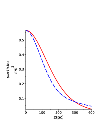
Figure 1: Profiles of density versus scale height $z$: the disk in presence of self-gravity as given by Eq. (8) when $h=90$ pc (dashed blue line) and the three-component exponential distribution as given by Eq. (3) (red full line).

The mass $M_{0}$ swept in the interval [0,$r_{0}$] is

$$M_{0}(\rho_{c},r_{0})=\frac{4}{3}\,\rho_{{c}}\pi\,{r_{{0}}}^{3}\quad.$$

The total mass $M(r;r_{0},\rho_{c},h)$ swept in the interval [0,r] is

$$M(r;r_{0},\rho_{c},h)={\frac{\rho_{{c}}{r_{{0}}}^{3}}{3}}-4\,{\frac{\rho_{{c}}{r}^{2}h}{\cos\left(\theta\right)}\left(1+{{\rm e}^{{\frac{r\cos\left(\theta\right)}{h}}}}\right)^{-1}}+4\,{\frac{\rho_{{c}}{r}^{2}h}{\cos\left(\theta\right)}}-8\,{\frac{\rho_{{c}}{h}^{2}r}{\left(\cos\left(\theta\right)\right)^{2}}\ln\left(1+{{\rm e}^{{\frac{r\cos\left(\theta\right)}{h}}}}\right)}$$

$$-8\,{\frac{\rho_{{c}}{h}^{3}}{\left(\cos\left(\theta\right)\right)^{3}}{\it polylog}\left(2,-{{\rm e}^{{\frac{r\cos\left(\theta\right)}{h}}}}\right)}+4\,{\frac{\rho_{{c}}{r_{{0}}}^{2}h}{\cos\left(\theta\right)}\left(1+{{\rm e}^{{\frac{r_{{0}}\cos\left(\theta\right)}{h}}}}\right)^{-1}}$$

$$-4\,{\frac{\rho_{{c}}{r_{{0}}}^{2}h}{\cos\left(\theta\right)}}+8\,{\frac{\rho_{{c}}{h}^{2}r_{{0}}}{\left(\cos\left(\theta\right)\right)^{2}}\ln\left(1+{{\rm e}^{{\frac{r_{{0}}\cos\left(\theta\right)}{h}}}}\right)}+8\,{\frac{\rho_{{c}}{h}^{3}}{\left(\cos\left(\theta\right)\right)^{3}}{\it polylog}\left(2,-{{\rm e}^{{\frac{r_{{0}}\cos\left(\theta\right)}{h}}}}\right)}$$ (10)

where $\theta$ is the polar angle and the polylog operator is defined by

$$polylog(s,z)=\mathrm{Li}_{s}\left(z\right)=\sum_{n=1}^{\infty}\frac{z^{n}}{n^{s}}\quad$$ (11)

where $\mathrm{Li}_{s}\left(z\right)$ is the Dirichlet series. The positive solution of Eq. (1) gives the velocity as a function of the radius:

$$v(r;r_{0},v_{0},h)=\frac{AN}{AD}\quad,$$ (12)

where

$$AN=-\Big{(}{-24\,\cos(\theta)r_{{0}}({{\rm e}^{{\frac{\cos(\theta)(r+r_{{0}})}{h}}}}+{{\rm e}^{{\frac{\cos(\theta)r_{{0}}}{h}}}}+{{\rm e}^{{\frac{r\cos(\theta)}{h}}}}+1)(-{h}^{3}({{\rm e}^{{\frac{\cos(\theta)(r+r_{{0}})}{h}}}}+{{\rm e}^{{\frac{\cos(\theta)r_{{0}}}{h}}}}+{{\rm e}^{{\frac{r\cos(\theta)}{h}}}}}$$

$$+1){{\it polylog}(2,-{{\rm e}^{{\frac{\cos(\theta)r_{{0}}}{h}}}})+{h}^{3}({{\rm e}^{{\frac{\cos(\theta)(r+r_{{0}})}{h}}}}+{{\rm e}^{{\frac{\cos(\theta)r_{{0}}}{h}}}}+{{\rm e}^{{\frac{r\cos(\theta)}{h}}}}+1){\it polylog}(2,-{{\rm e}^{{\frac{r\cos(\theta)}{h}}}})}$$

$${+\cos(\theta)((-{h}^{2}r_{{0}}\ln(1+{{\rm e}^{{\frac{\cos(\theta)r_{{0}}}{h}}}})+{h}^{2}r\ln(1+{{\rm e}^{{\frac{r\cos(\theta)}{h}}}})-1/2\,\cos(\theta)(1/12\,{r_{{0}}}^{3}\cos(\theta)+h{r}^{2}-h{r_{{0}}}^{2}))}$$

$${{{\rm e}^{{\frac{\cos(\theta)(r+r_{{0}})}{h}}}}-{h}^{2}r_{{0}}({{\rm e}^{{\frac{\cos(\theta)r_{{0}}}{h}}}}+{{\rm e}^{{\frac{r\cos(\theta)}{h}}}}+1)\ln(1+{{\rm e}^{{\frac{\cos(\theta)r_{{0}}}{h}}}})+{h}^{2}r({{\rm e}^{{\frac{\cos(\theta)r_{{0}}}{h}}}}+{{\rm e}^{{\frac{r\cos(\theta)}{h}}}}+1)\times}$$

$${\ln(1+{{\rm e}^{{\frac{r\cos(\theta)}{h}}}})-1/2\,\cos(\theta)((1/12\,{r_{{0}}}^{3}\cos(\theta)-h{r_{{0}}}^{2}){{\rm e}^{{\frac{\cos(\theta)r_{{0}}}{h}}}}}$$

$${+(1/12\,{r_{{0}}}^{3}\cos(\theta)+h{r}^{2}){{\rm e}^{{\frac{r\cos(\theta)}{h}}}}+1/12\,{r_{{0}}}^{3}\cos(\theta))))}\Big{)}^{1/2}\cos(\theta){\it v_{0}}\,r_{{0}}$$ (13)

and

$$AD=-{r_{{0}}}^{3}{{\rm e}^{{\frac{\cos\left(\theta\right)\left(r+r_{{0}}\right)}{h}}}}\left(\cos\left(\theta\right)\right)^{3}+24\,{h}^{2}r{{\rm e}^{{\frac{\cos\left(\theta\right)\left(r+r_{{0}}\right)}{h}}}}\ln\left(1+{{\rm e}^{{\frac{r\cos\left(\theta\right)}{h}}}}\right)\cos\left(\theta\right)$$

$$-24\,{h}^{2}r_{{0}}{{\rm e}^{{\frac{\cos\left(\theta\right)\left(r+r_{{0}}\right)}{h}}}}\ln\left(1+{{\rm e}^{{\frac{\cos\left(\theta\right)r_{{0}}}{h}}}}\right)\cos\left(\theta\right)-12\,h{r}^{2}{{\rm e}^{{\frac{\cos\left(\theta\right)\left(r+r_{{0}}\right)}{h}}}}\left(\cos\left(\theta\right)\right)^{2}$$

$$+12\,h{r_{{0}}}^{2}{{\rm e}^{{\frac{\cos\left(\theta\right)\left(r+r_{{0}}\right)}{h}}}}\left(\cos\left(\theta\right)\right)^{2}-{r_{{0}}}^{3}{{\rm e}^{{\frac{r\cos\left(\theta\right)}{h}}}}\left(\cos\left(\theta\right)\right)^{3}-{r_{{0}}}^{3}{{\rm e}^{{\frac{\cos\left(\theta\right)r_{{0}}}{h}}}}\left(\cos\left(\theta\right)\right)^{3}$$

$$+24\,{h}^{3}{{\rm e}^{{\frac{\cos\left(\theta\right)\left(r+r_{{0}}\right)}{h}}}}{\it polylog}\left(2,-{{\rm e}^{{\frac{r\cos\left(\theta\right)}{h}}}}\right)-24\,{h}^{3}{{\rm e}^{{\frac{\cos\left(\theta\right)\left(r+r_{{0}}\right)}{h}}}}{\it polylog}\left(2,-{{\rm e}^{{\frac{\cos\left(\theta\right)r_{{0}}}{h}}}}\right)$$

$$+24\,{h}^{2}r{{\rm e}^{{\frac{r\cos\left(\theta\right)}{h}}}}\ln\left(1+{{\rm e}^{{\frac{r\cos\left(\theta\right)}{h}}}}\right)\cos\left(\theta\right)+24\,{h}^{2}r{{\rm e}^{{\frac{\cos\left(\theta\right)r_{{0}}}{h}}}}\ln\left(1+{{\rm e}^{{\frac{r\cos\left(\theta\right)}{h}}}}\right)\cos\left(\theta\right)$$

$$-24\,{h}^{2}r_{{0}}{{\rm e}^{{\frac{r\cos\left(\theta\right)}{h}}}}\ln\left(1+{{\rm e}^{{\frac{\cos\left(\theta\right)r_{{0}}}{h}}}}\right)\cos\left(\theta\right)-24\,{h}^{2}r_{{0}}{{\rm e}^{{\frac{\cos\left(\theta\right)r_{{0}}}{h}}}}\ln\left(1+{{\rm e}^{{\frac{\cos\left(\theta\right)r_{{0}}}{h}}}}\right)\cos\left(\theta\right)$$

$$-12\,h{r}^{2}{{\rm e}^{{\frac{r\cos\left(\theta\right)}{h}}}}\left(\cos\left(\theta\right)\right)^{2}+12\,h{r_{{0}}}^{2}{{\rm e}^{{\frac{\cos\left(\theta\right)r_{{0}}}{h}}}}\left(\cos\left(\theta\right)\right)^{2}-{r_{{0}}}^{3}\left(\cos\left(\theta\right)\right)^{3}$$

$$+24\,{h}^{3}{{\rm e}^{{\frac{r\cos\left(\theta\right)}{h}}}}{\it polylog}\left(2,-{{\rm e}^{{\frac{r\cos\left(\theta\right)}{h}}}}\right)-24\,{h}^{3}{{\rm e}^{{\frac{r\cos\left(\theta\right)}{h}}}}{\it polylog}\left(2,-{{\rm e}^{{\frac{\cos\left(\theta\right)r_{{0}}}{h}}}}\right)$$

$$+24\,{h}^{3}{{\rm e}^{{\frac{\cos\left(\theta\right)r_{{0}}}{h}}}}{\it polylog}\left(2,-{{\rm e}^{{\frac{r\cos\left(\theta\right)}{h}}}}\right)-24\,{h}^{3}{{\rm e}^{{\frac{\cos\left(\theta\right)r_{{0}}}{h}}}}{\it polylog}\left(2,-{{\rm e}^{{\frac{\cos\left(\theta\right)r_{{0}}}{h}}}}\right)$$

$$+24\,{h}^{2}r\ln\left(1+{{\rm e}^{{\frac{r\cos\left(\theta\right)}{h}}}}\right)\cos\left(\theta\right)-24\,{h}^{2}r_{{0}}\ln\left(1+{{\rm e}^{{\frac{\cos\left(\theta\right)r_{{0}}}{h}}}}\right)\cos\left(\theta\right)$$

$$+24\,{h}^{3}{\it polylog}\left(2,-{{\rm e}^{{\frac{r\cos\left(\theta\right)}{h}}}}\right)-24\,{h}^{3}{\it polylog}\left(2,-{{\rm e}^{{\frac{\cos\left(\theta\right)r_{{0}}}{h}}}}\right)$$ (14)

The differential equation which governs the motion for the medium in the presence of self-gravity is

$$\Big{(}{\frac{\rho_{{c}}{r_{{0}}}^{3}}{3}}-4\,{\frac{\rho_{{c}}(r(t))^{2}h}{\cos(\theta)}(1+{{\rm e}^{{\frac{r(t)\cos(\theta)}{h}}}})^{-1}}+4\,{\frac{\rho_{{c}}(r(t))^{2}h}{\cos(\theta)}}$$

$$-8\,{\frac{\rho_{{c}}{h}^{2}r(t)}{(\cos(\theta))^{2}}\ln(1+{{\rm e}^{{\frac{r(t)\cos(\theta)}{h}}}})}-8\,{\frac{\rho_{{c}}{h}^{3}}{(\cos(\theta))^{3}}{\it polylog}(2,-{{\rm e}^{{\frac{r(t)\cos(\theta)}{h}}}})}+4\,{\frac{\rho_{{c}}{r_{{0}}}^{2}h}{\cos(\theta)}(1+{{\rm e}^{{\frac{r_{{0}}\cos(\theta)}{h}}}})^{-1}}$$

$$-4\,{\frac{\rho_{{c}}{r_{{0}}}^{2}h}{\cos(\theta)}}+8\,{\frac{\rho_{{c}}{h}^{2}r_{{0}}}{(\cos(\theta))^{2}}\ln(1+{{\rm e}^{{\frac{r_{{0}}\cos(\theta)}{h}}}})}+8\,{\frac{\rho_{{c}}{h}^{3}}{(\cos(\theta))^{3}}{\it polylog}(2,-{{\rm e}^{{\frac{r_{{0}}\cos(\theta)}{h}}}})}\Big{)}\Big{(}{\frac{\rm d}{{\rm d}t}}r(t)\Big{)}^{2}$$

$$-{\frac{\rho_{{c}}{r_{{0}}}^{3}{v_{{0}}}^{2}}{3}}=0\quad,$$ (15)

and does not have an analytical solution. Figure 2 shows the numerical solution obtained with the Runge–Kutta method.

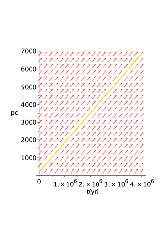
Figure 2: Phase plane portrait and numerical solution (full yellow line) for a medium in the presence of self-gravity as given by Eq. (8) when $r_{0}=250$ pc, $h=90$ pc, $t=4\,10^{6}$ yr, $t_{0}=4\,10^{4}$ yr and $v_{0}\,=2000$ km s^-1.

A Taylor expansion of order 3 of Eq. (15) gives

$$r(t;t_{0},v_{0},r_{0},h)=r_{{0}}+v_{{0}}\left(t-t_{{0}}\right)-3\,{\frac{{v_{{0}}}^{2}\left(t-t_{{0}}\right)^{2}}{r_{{0}}}{{\rm e}^{{\frac{r_{{0}}\cos\left(\theta\right)}{h}}}}\left(\left({{\rm e}^{{\frac{r_{{0}}\cos\left(\theta\right)}{h}}}}\right)^{2}+2\,{{\rm e}^{{\frac{r_{{0}}\cos\left(\theta\right)}{h}}}}+1\right)^{-1}}\quad,$$ (16)

and Figure 3 shows the numerical solution obtained by the Runge–Kutta method and the series solution up to a time for which the percentage error is less than $10\%$.

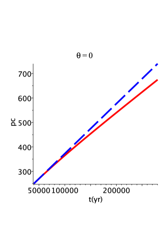
Figure 3: Numerical solution (red full line) and Taylor expansion of the solution (dashed blue line), parameters as in Figure 2 but $t=2.8\,10^{5}$ yr,

2.3 Gaussian medium

We assume that the number density distribution scales as

$$n(z)=n_{0}{{\rm e}^{-{\frac{{z}^{2}}{{z_{{0}}}^{2}}}}}\quad,$$ (17)

where $n_{0}$ is the density at $z=0$ and $z_{0}$ is a scaling parameter. We now give the adopted piece-wise dependence for the Gaussian medium

$$\rho(r;r_{0},z_{0})=\Bigg{\{}\begin{array}[]{ll}\rho_{c}&\mbox{if $r\leq r_{0}$ }\\ \rho_{c}\,{{\rm e}^{-{\frac{{r}^{2}\left(\cos\left(\theta\right)\right)^{2}}{{{\it z_{0}}}^{2}}}}}&\mbox{if $r>r_{0}$}\end{array}\quad,$$ (18)

where $\rho_{c}$ is the density at $z=0$. A comparison with Eq. (3) gives $z_{0}=200$ pc, see Figure 4.

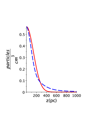
Figure 4: Profiles of density versus scale height $z$: the medium is that in the presence of a Gaussian medium as given by Eq. (17) when $h=90$ pc (dashed blue line) and the three-component exponential distribution as given by Eq. (3) (red full line).

The total mass $M(r;r_{0},\rho_{c},z_{0})$ swept in the interval [0,r] is

$$M(r;r_{0},\rho_{c},z_{0})=\frac{BN}{12\,\left(\cos\left(\theta\right)\right)^{3}}\quad,$$ (19)

where

$$BN=-\Bigg{(}-4\,{r_{{0}}}^{3}\left(\cos\left(\theta\right)\right)^{3}+3\,{\rm erf}\left({\frac{r_{{0}}\cos\left(\theta\right)}{z_{{0}}}}\right)\sqrt{\pi}{z_{{0}}}^{3}-3\,{\rm erf}\left({\frac{r\cos\left(\theta\right)}{z_{{0}}}}\right)\sqrt{\pi}{z_{{0}}}^{3}$$

$$+6\,{{\rm e}^{-{\frac{{r}^{2}\left(\cos\left(\theta\right)\right)^{2}}{{z_{{0}}}^{2}}}}}\cos\left(\theta\right)r{z_{{0}}}^{2}-6\,{{\rm e}^{-{\frac{{r_{{0}}}^{2}\left(\cos\left(\theta\right)\right)^{2}}{{z_{{0}}}^{2}}}}}\cos\left(\theta\right)r_{{0}}{z_{{0}}}^{2}\Bigg{)}\rho_{{c}}\quad,$$ (20)

and erf$(x)$ [28] is the error function defined by

$${\rm erf}(x)=2\,{\frac{\int_{0}^{x}\!{\it\exp}\left(-{t}^{2}\right)\,{\rm d}t}{\sqrt{\pi}}}\quad.$$ (21)

The velocity as a function of the radius is

$$v(r;r_{0},z_{0},v_{0})=\frac{CN}{CD}\quad,$$ (22)

where

$$CN=2\,\Bigg{(}{-6\,\cos(\theta)(-2/3\,{r_{{0}}}^{3}(\cos(\theta))^{3}+{{\rm e}^{-{\frac{{r}^{2}(\cos(\theta))^{2}}{{z_{{0}}}^{2}}}}}\cos(\theta)r{z_{{0}}}^{2}-{{\rm e}^{-{\frac{{r_{{0}}}^{2}(\cos(\theta))^{2}}{{z_{{0}}}^{2}}}}}\cos(\theta)r_{{0}}{z_{{0}}}^{2}}$$

$${-1/2\,{\rm erf}({\frac{\cos(\theta)r}{z_{{0}}}})\sqrt{\pi}{z_{{0}}}^{3}+1/2\,{\rm erf}({\frac{r_{{0}}\cos(\theta)}{z_{{0}}}})\sqrt{\pi}{z_{{0}}}^{3})r_{{0}}}\Bigg{)}^{1/2}\cos(\theta)v_{{0}}r_{{0}}\quad,$$ (23)

and

$$CD=4\,{r_{{0}}}^{3}\left(\cos\left(\theta\right)\right)^{3}-6\,{{\rm e}^{-{\frac{{r}^{2}\left(\cos\left(\theta\right)\right)^{2}}{{z_{{0}}}^{2}}}}}\cos\left(\theta\right)r{z_{{0}}}^{2}+6\,{{\rm e}^{-{\frac{{r_{{0}}}^{2}\left(\cos\left(\theta\right)\right)^{2}}{{z_{{0}}}^{2}}}}}\cos\left(\theta\right)r_{{0}}{z_{{0}}}^{2}$$

$$-3\,{\rm erf}\left({\frac{r_{{0}}\cos\left(\theta\right)}{z_{{0}}}}\right)\sqrt{\pi}{z_{{0}}}^{3}+3\,{\rm erf}\left({\frac{\cos\left(\theta\right)r}{z_{{0}}}}\right)\sqrt{\pi}{z_{{0}}}^{3}\quad.$$ (24)

The differential equation which governs the motion for the Gaussian medium is

$$4\,\left(\cos\left(\theta\right)\right)^{3}\left({\frac{\rm d}{{\rm d}t}}r\left(t\right)\right)^{2}{r_{{0}}}^{3}-4\,{r_{{0}}}^{3}{v_{{0}}}^{2}\left(\cos\left(\theta\right)\right)^{3}-6\,r\left(t\right)\cos\left(\theta\right){{\rm e}^{-{\frac{\left(r\left(t\right)\right)^{2}\left(\cos\left(\theta\right)\right)^{2}}{{z_{{0}}}^{2}}}}}\left({\frac{\rm d}{{\rm d}t}}r\left(t\right)\right)^{2}{z_{{0}}}^{2}$$

$$+6\,\cos\left(\theta\right){{\rm e}^{-{\frac{{r_{{0}}}^{2}\left(\cos\left(\theta\right)\right)^{2}}{{z_{{0}}}^{2}}}}}\left({\frac{\rm d}{{\rm d}t}}r\left(t\right)\right)^{2}r_{{0}}{z_{{0}}}^{2}-3\,\sqrt{\pi}{\rm erf}\left({\frac{r_{{0}}\cos\left(\theta\right)}{z_{{0}}}}\right)\left({\frac{\rm d}{{\rm d}t}}r\left(t\right)\right)^{2}{z_{{0}}}^{3}$$

$$+3\,\sqrt{\pi}{\rm erf}\left({\frac{r\left(t\right)\cos\left(\theta\right)}{z_{{0}}}}\right)\left({\frac{\rm d}{{\rm d}t}}r\left(t\right)\right)^{2}{z_{{0}}}^{3}=0\quad.$$ (25)

Figure 5 shows the numerical solution obtained with the Runge–Kutta method.

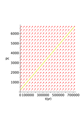
Figure 5: Phase plane portrait and numerical solution (full yellow line) in the Gaussian case when $r_{0}=250$ pc, $z_{0}=90$ pc, $t=7.1\,10^{5}$ yr, $t_{0}=7.1\,10^{3}$ yr and $v_{0}\,=10000$ km s^-1.

A Taylor expansion of order 3 of Eq. (25) gives

$$r(t;t_{0},r_{0},v_{0},z_{0})=r_{{0}}+v_{{0}}\left(t-t_{{0}}\right)-{\frac{3\,{v_{{0}}}^{2}\left(t-t_{{0}}\right)^{2}}{4\,r_{{0}}}{{\rm e}^{-{\frac{{r_{{0}}}^{2}\left(\cos\left(\theta\right)\right)^{2}}{{z_{{0}}}^{2}}}}}}\quad,$$ (26)

and Figure 6 gives the numerical solution obtained by the Runge–Kutta method and the series solution up to a time for which the percentage error is less than $9\%$.

Figure 6: Numerical solution (red full line) and Taylor expansion of the solution (dashed blue line), parameters as in Figure 5 but $t=4.26\,10^{4}$ yr,

3 Astrophysical applications

In the following we will analyse the local bubble, the Fermi bubble and the super bubble W4. An observational percentage reliability, $\epsilon_{\mathrm{obs}}$, is introduced over the whole range of the polar angle $\theta$,

$$\epsilon_{\mathrm{obs}}=100(1-\frac{\sum_{j}|r_{\mathrm{obs}}-r_{\mathrm{num}}|_{j}}{\sum_{j}{r_{\mathrm{obs}}}_{,j}})\quad,$$ (27)

where $r_{\mathrm{num}}$ is the theoretical radius of the considered bubble, $r_{\mathrm{obs}}$ is the observed radius of the considered bubble, and the index $j$ varies from 1 to the number of available observations. The observational percentage of reliability allows us to fix the theoretical parameters.

3.1 The local bubble

The local bubble (LB) has already been simulated in the framework of the conservation of momentum [29]; here we adopt the framework of the conservation of energy. The numerical solution is shown as a cut in the $x-z$ plane: see Figure 7 for a medium in the presence of self-gravity as given by Eq. (9) and Figure 8 for a Gaussian density profile as given by Eq. (18).

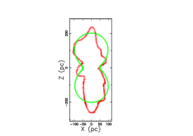
Figure 7: Geometrical section of the LB in the $x-z$ plane with a profile in the presence of self-gravity as given by Eq. (8) (green points) and observed profile (red stars). The parameters are $v_{0}\,=3700$ km s^-1, $r_{0}\,=7$ pc, $h\,=3.5$ pc, $t=8.5\,10^{4}$ yr, $t_{0}=8.5\,10^{2}$ yr and $z_{OB}=0$. The observational percentage reliability is $\epsilon_{\mathrm{obs}}=82.42\%$.

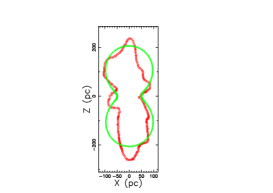
Figure 8: Geometrical section of the LB in the $x-z$ plane with a Gaussian profile (green points) and observed profile (red stars). The parameters are $v_{0}\,=4000$ km s^-1, $r_{0}\,=7$ pc, $z_{0}\,=9.1$ pc, $t=8.5\,10^{4}$ yr, $t_{0}=8.5\,10^{2}$ yr and $z_{OB}=0$ . The observational percentage reliability is $\epsilon_{\mathrm{obs}}=82.58\%$.

The 3D advancing surface of the local bubble for the case of self-gravity is shown in Figure 9.

Figure 9: 3D surface of the LB with parameters as in Figure 7, with a profile in presence of self-gravity as given by Eq. (8). The three Euler angles are $\Theta=90^{\circ}$, $\Phi=0^{\circ}$ and $\Psi=90^{\circ}$.

3.2 The Fermi bubble

Fermi bubbles have already been simulated in the framework of the conservation of momentum [30]; here we apply the conservation of energy. We now test our models on the image of the Fermi bubbles available at https://www.nasa.gov/mission_pages/GLAST/news/new-structure.html. The numerical solution is shown as a cut in the $x-z$ plane: see Figure 10 for a density profile in the presence of self-gravity

as given by Eq. (9) and Figure 11 for a Gaussian density profile as given by Eq. (18).

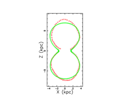
Figure 10: Geometrical section of the Fermi bubbles in the $x-z$ plane with a profile in the presence of self-gravity as given by Eq. (8) (green points) and observed profile (red stars). The parameters are $v_{0}\,=2000$ km s^-1, $r_{0}\,=250$ pc, $z_{0}\,=12$ pc, $t=4\,10^{6}$ yr, $t_{0}=4\,10^{4}$ yr and $z_{OB}=0$. The observational percentage reliability is $\epsilon_{\mathrm{obs}}=93\%$.

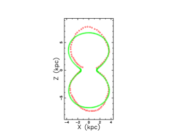
Figure 11: Geometrical section of the Fermi bubbles in the $x-z$ plane with a Gaussian profile (green points) and observed profile (red stars). The parameters are $v_{0}\,=1000$ km s^-1, $r_{0}\,=250$ pc, $z_{0}\,=200$ pc, $t=7.1\,10^{5}$ yr, $t_{0}=7.1\,10^{3}$ yr and $z_{OB}=0$. The observational percentage reliability is $\epsilon_{\mathrm{obs}}=92.12\%$.

The 3D advancing surface of the local bubble for the Gaussian case is shown in Figure 12.

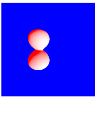
Figure 12: 3D surface of the Fermi bubbles with parameters as in Figure 11, Gaussian profile. The three Euler angles are $\Theta=90^{\circ}$, $\Phi=0^{\circ}$ and $\Psi=90^{\circ}$.

3.3 The W4 super-bubble

The W4 super-bubble has been analysed from the point of view of the astronomical observations [31, 32, 33], in connection with the evolution of the magnetic field [34] and from a theoretical point of view [9, 35]. The upper part of Figure 3 in [36], which combines [SII], $H\alpha$ and [OIII] images has been digitized and will be the section of reference for W4, see Figure 13.

Figure 13: Section of the W4 + IC 1805 complex.

We now simulate the egg-shape of W4 when $z_{OB}\neq 0$. The numerical solution, which is evaluated with the Euler method, is shown as a cut in the $x-z$ plane: see Figure 14 for a density profile in the presence of self-gravity and Figure 15 for a Gaussian profile. The two adopted profiles in density are symmetric with respect to the galactic plane, $Z=0$, but the simulated theoretical sections do not have an up–down symmetry, due to the fact that the expansion starts at $z=z_{0}$. Nevertheless, we still have a right–left symmetry.

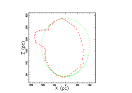
Figure 14: Geometrical section of the W4 super-bubble in the $X-Z$ plane with a profile in the presence of self-gravity as given by Eq. (8) (green points) and observed profile (red stars). The parameters are $v_{0}\,=20000$ km s^-1, $r_{0}\,=1$ pc, $h\,=17$ pc, $t=1.3\,10^{5}$ yr, $t_{0}=10$ yr and $z_{OB}=100$.

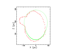
Figure 15: Geometrical section of the W4 super-bubble in the $X-Z$ plane with a Gaussian profile (green points) and observed profile (red stars). The parameters are $v_{0}\,=4700$ km s^-1, $r_{0}\,=1$ pc, $z_{0}\,=55$ pc, $t=2.25\,10^{5}$ yr, $t_{0}=10$ yr and $z_{OB}=100$.

The egg shape of the W4 super-bubble is shown in Figure 16.

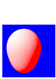
Figure 16: 3D surface of the W4 super-bubble with parameters as in Figure 15, Gaussian profile. The three Euler angles are $\Theta=90^{\circ}$, $\Phi=0^{\circ}$ and $\Psi=90^{\circ}$.

The curious bump visible in the upper left part of Figure 13 could be an astronomical superposition of the image of IC 1805 on W4 or an intrinsic feature in the expansion of W4. In order to reproduce this feature, we assume that the scaling factor $z_{0,\theta}$ in the interval $\theta_{inf}<\theta<\theta_{sup}$ varies with the following empirical law

$$z_{0,\theta}=z_{0}+z0\,0.0006N(\theta;\overline{\theta},\sigma)$$ (28)

where

$$N(\theta;\sigma,\mu)=\frac{1}{\sigma(2\pi)^{1/2}}\exp({-{\frac{(x-\overline{\theta})^{2}}{2\sigma^{2}}}})\quad,$$ (29)

is the Gaussian distribution, and $\overline{\theta}=\frac{\theta_{inf}+\theta_{sup}}{2}$ and $\sigma=\overline{\theta}/9$.

Figure 17 shows an ‘ad hoc’ simulation of the bump of W4.

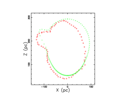
Figure 17: Geometrical section of the W4 super-bubble in the $X-Z$ plane with a Gaussian profile (green points) and observed profile (red stars). The parameters are the same as for Figure 15.

4 The theory of the image

In the framework of an optically thin medium, we outline a new analytical model which reproduces a theoretical vertical cut in the intensity of radiation and an old numerical model which simulates the intensity of radiation as a function of the point of view of the observer.

4.1 The piriform model

The piriform curve, or pear-shaped quartic, in 3D Cartesian coordinates $(x,y,z)$ has the equation

$${a}^{4}\left({x}^{2}+{y}^{2}\right)-{b}^{2}{z}^{3}\left(2\,a-z\right)=0\quad,$$ (30)

where $a$ and $b$ are both positive [37], see Figure 18 where the parameters $a$ and $b$ match the Fermi bubbles.

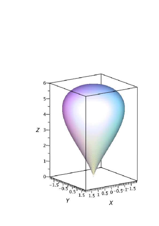
Figure 18: 3D display of the piriform curve when $a=3$ kpc and $b=3/2$ kpc.

We are interested in a section of the above curve in the $x-z$ plane which is obtained by inserting $y=0$

$${a}^{4}{x}^{2}={b}^{2}{z}^{3}\left(2\,a-z\right)\quad.$$ (31)

The parametric form of the piriform curve is

$$x(\theta;a,b)=a\left(1+\sin\left(\theta\right)\right)$$ (32a)

$$z(\theta;a,b)=b\cos\left(\theta\right)\left(1+\sin\left(\theta\right)\right)\quad,$$ (32b)

where $-\frac{\pi}{2}\leq\theta\leq\frac{3\pi}{2}$ and the maximum value reached along the $z$ axis is

$$z_{max}=2\,a\quad.$$ (33)

We assume that the emission takes place in a thin layer comprised between an internal piriform which in polar coordinates has radius

$$r_{int}={\frac{z}{{a}^{2}}\sqrt{{a}^{4}+2\,a{b}^{2}z-{b}^{2}{z}^{2}}}\quad,$$ (34)

and an external piriform which has radius

$$r_{ext}=r_{int}+c\quad,$$ (35)

where $c$ is a positive parameter, see Figure 19.

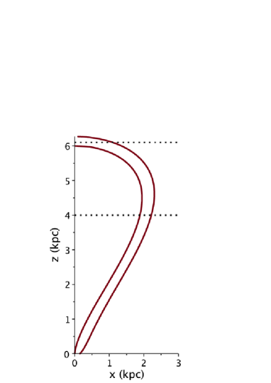
Figure 19: Internal and external piriforms in the first quadrant when $a=3$ kpc, $b=3/2$ kpc and $c=3/20$. The dotted lines represent two different lengths of sight.

We therefore assume that the number density $C_{m}$ is constant between the two piriforms; as an example, along the $z$ axis the number density increases from 0 at $(0,z_{max})$ to a maximum value $C_{m}$, remains constant up to $(0,z_{max}+c)$, and then falls again to 0. The length of sight which produces the image in the first quadrant, when the observer is situated at the infinity of the $x$-axis, is the locus parallel to the $x$-axis which crosses the position $z$ in the Cartesian $x-z$ plane and terminates at the external piriform. In the case of an optically thin medium, the line of sight is split into two cases

$$l_{I}(z;a,b,c,C_{m})=$$

$$\frac{1}{{a}^{2}}\Bigg{(}C_{{m}}\sqrt{{a}^{4}{c}^{2}+2\,{b}^{2}{z}^{3}a-{b}^{2}{z}^{4}+2\,\sqrt{\left(2\,az-{z}^{2}\right){b}^{2}+{a}^{4}}{a}^{2}cz}\Bigg{)}$$ (36)

$$when\quad z_{max}\leq z<z_{max}+c$$

$$l_{II}(z;a,b,c,C_{m})=$$

$$\frac{1}{{a}^{2}}\Bigg{(}-C_{{m}}\left(\sqrt{z\left(2\,a-z\right)}zb-\sqrt{{a}^{4}{c}^{2}+2\,{b}^{2}{z}^{3}a-{b}^{2}{z}^{4}+2\,\sqrt{\left(2\,az-{z}^{2}\right){b}^{2}+{a}^{4}}{a}^{2}cz}\right)\Bigg{)}$$ (37)

$$when\quad 0\leq z<z_{max}\quad.$$

A comparison between observed and theoretical intensity can be made by replacing in the above result $C_{m}$ with $I_{m}$ and doubling the length of sight due to the contribution of the second quadrant

$$I_{I}(z;a,b,c,I_{m})=$$

$$2\times\frac{1}{{a}^{2}}\Bigg{(}I_{{m}}\sqrt{{a}^{4}{c}^{2}+2\,{b}^{2}{z}^{3}a-{b}^{2}{z}^{4}+2\,\sqrt{\left(2\,az-{z}^{2}\right){b}^{2}+{a}^{4}}{a}^{2}cz}\Bigg{)}$$ (38)

$$when\quad z_{max}\leq z<z_{max}+c$$

$$I_{II}(z;a,b,c,I_{m})=$$

$$2\times\frac{1}{{a}^{2}}\Bigg{(}-I_{{m}}\left(\sqrt{z\left(2\,a-z\right)}zb-\sqrt{{a}^{4}{c}^{2}+2\,{b}^{2}{z}^{3}a-{b}^{2}{z}^{4}+2\,\sqrt{\left(2\,az-{z}^{2}\right){b}^{2}+{a}^{4}}{a}^{2}cz}\right)\Bigg{)}$$ (39)

$$when\quad 0\leq z<z_{max}\quad.$$

The resulting intensity is $I_{{m}}\,2\,c$ at $z=0$ and increases to $I_{{m}}\,2\,\sqrt{c}\sqrt{4\,a+c}$ at $z=z_{max}$, see Figure 20 for a typical profile in intensity along the $z$-axis.

Figure 20: The intensity profile for the piriform model along the $z$-axis when when $a=3$ kpc, $b=3/2$ kpc, $c=3/20$ and $C_{m}$=1.

4.2 The numerical model

The source of the luminosity is assumed here to be the flux of kinetic energy, $L_{m}$. The observed luminosity along a given direction can be expressed as

$$L=\epsilon L_{m}\quad,$$ (40)

where $\epsilon$ is a constant of conversion from the mechanical luminosity to the observed luminosity, for more details see [30]. The image of the Fermi bubbles is shown in Figure 21 and Figure 22 shows a cut of the intensity along the $z$-axis.

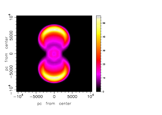
Figure 21: Map of the theoretical intensity of the Fermi bubbles for the model in the presence of self-gravity as given by Eq. (8) with parameters as in Figure 10. The three Euler angles characterizing the orientation are $\Phi$=0^∘, $\Theta$=90^∘ and $\Psi$=90^∘.

Figure 22 also shows the cut of the piriform model in order to evaluate the goodness of the analytical model for complex sections.

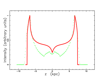
Figure 22: The intensity profile for the Fermi bubbles evolving in a model in the presence of self-gravity as given by Eq. (8) along the $z$-axis, parameters as in Figure 21 (green empty stars) and the intensity profile for the piriform model along the $z$-axis when when $a=3.3$ kpc, $b=1.65$ kpc, $c=0.825$ and $C_{m}$=1 (red full line).

5 Conclusions

Equations of motion We derived two equations of motion coupling the thin layer approximation with the conservation of energy. The first model implements a profile in the presence of self-gravity of density and the second a Gaussian profile of density. In the absence of analytical results for the trajectory, with the exception of a Taylor expansion, we provided a numerical solution.

Comparison with other approaches

As an example, Figure 3 in [13] models the Eridanus–Orion structure with an ellipsoid, here we introduce the mushroom shape, see Figure 10 relative to the Fermi bubble and the egg shape, see Figure 16 relative to W4. We also suggested a first model for shapes apparently impossible to be simulated, see Figure 17 for the bump of W4.

Theory of the image The introduction of the piriform curve as a model for the section of the super-bubble confirms the existence of a characteristic ‘U’ shape which has a maximum in the internal piriform at $z=2\,a$ and a minimum at the centre, $z=0$, see Eq. (20). The superposition of a numerical cut with the piriform’s cut, see Figure 22, shows us that the use of the piriform curve as a model is acceptable.

References

- [1] Heiles C 1979 H I shells and supershells ApJ 229, 533
- [2] Cash W, Charles P, Bowyer S, Walter F, Garmire G and Riegler G 1980 The X-ray superbubble in Cygnus. ApJ Letters, 238, L71
- [3] Heiles C 1984 HI shells, supershells, shell-like objects, and “worms”. ApJS 55, 585
- [4] Tenorio-Tagle G and Bodenheimer P 1988 Large-scale expanding superstructures in galaxies ARA&A 26, 145
- [5] McCray R A 1987 Coronal interstellar gas and supernova remnants in A Dalgarno & D Layzer, eds, Spectroscopy of Astrophysical Plasmas (Cambridge: Cambridge University Press) pp. 255–278
- [6] McCray R and Kafatos M 1987 Supershells and propagating star formation ApJ 317, 190
- [7] Mac Low M M and McCray R 1988 Superbubbles in disk galaxies ApJ 324, 776
- [8] Igumenshchev I V, Shustov B M and Tutukov A V 1990 Dynamics of supershells – Blow-out A&A 234, 396
- [9] Basu S, Johnstone D and Martin P G 1999 Dynamical Evolution and Ionization Structure of an Expanding Superbubble: Application to W4 ApJ 516, 843 (Preprint astro-ph/9812283)
- [10] Kompaneyets A S 1960 A Point Explosion in an Inhomogeneous Atmosphere Soviet Phys. Dokl. 5, 46
- [11] Olano C A 2009 The propagation of the shock wave from a strong explosion in a plane-parallel stratified medium: the Kompaneets approximation A&A 506, 1215
- [12] Pon A, Johnstone D, Bally J and Heiles C 2014 Kompaneets model fitting of the Orion–Eridanus superbubble MNRAS 444(4), 3657 (Preprint 1408.4454)
- [13] Pon A, Ochsendorf B B, Alves J, Bally J, Basu S and Tielens A G G M 2016 Kompaneets Model Fitting of the Orion–Eridanus Superbubble. II. Thinking Outside of Barnard’s Loop ApJ 827(1) 42 (Preprint 1606.02296)
- [14] Mac Low M M, McCray R and Norman M L 1989 Superbubble blowout dynamics ApJ 337, 141
- [15] Melioli C, Brighenti F, D’Ercole A and de Gouveia Dal Pino E M 2009 Hydrodynamical simulations of Galactic fountains – II. Evolution of multiple fountains MNRAS 399, 1089 (Preprint 0903.0720)
- [16] Soler J D, Bracco A and Pon A 2018 The magnetic environment of the Orion–Eridanus superbubble as revealed by Planck A&A 609 L3 (Preprint 1712.03728)
- [17] Tomisaka K 1992 The evolution of a magnetized superbubble PASJ 44, 177
- [18] Rafikov R R and Kulsrud R M 2000 Magnetic flux expulsion in powerful superbubble explosions and the - dynamo MNRAS 314, 839 (Preprint arXiv:astro-ph/0004084)
- [19] Bisnovatyi-Kogan G S and Silich S A 1995 Shock-wave propagation in the nonuniform interstellar medium Rev. Mod. Phys. 67, 661
- [20] Dickey J M and Lockman F J 1990 H I in the Galaxy ARA&A 28, 215
- [21] Lockman F J 1984 The H I halo in the inner galaxy ApJ 283, 90
- [22] Tenenbaum M and Pollard H 1963 Ordinary Differential Equations: An Elementary Textbook for Students of Mathematics, Engineering, and the Sciences (New York: Dover)
- [23] Ince E L 2012 Ordinary Differential Equations (New York: Dover)
- [24] Spitzer Jr L 1942 The Dynamics of the Interstellar Medium. III. Galactic Distribution. ApJ 95, 329
- [25] Rohlfs K, ed 1977 Lectures on Density Wave Theory vol. 69 of Lecture Notes in Physics, (Berlin: Springer-Verlag)
- [26] Bertin G 2000 Dynamics of Galaxies (Cambridge: Cambridge University Press.)
- [27] Padmanabhan P 2002 Theoretical Astrophysics. Vol. III: Galaxies and Cosmology (Cambridge: Cambridge University Press)
- [28] Olver F W J, Lozier D W, Boisvert R F and Clark C W 2010 NIST Handbook of Mathematical Functions (Cambridge: Cambridge University Press.)
- [29] Zaninetti L 2020 On the Shape of the Local Bubble International Journal of Astronomy and Astrophysics 10(1), 11 (Preprint 2002.02828)
- [30] Zaninetti L 2018 The Fermi Bubbles as a Superbubble International Journal of Astronomy and Astrophysics 8, 200 (Preprint 1806.09092)
- [31] Normandeau M and Basu S 1999 Observations and Modeling of the Disk-Halo Interaction in Our Galaxy in A R Taylor, T L Landecker and G Joncas, eds, New Perspectives on the Interstellar Medium vol. 168 of Astronomical Society of the Pacific Conference Series p. 287 (Preprint astro-ph/9811238)
- [32] Normandeau M 2000 The W4 Chimney/Superbubble in D Alloin, K Olsen and G Galaz, eds, Stars, Gas and Dust in Galaxies: Exploring the Links vol. 221 of Astronomical Society of the Pacific Conference Series p. 41 (Preprint astro-ph/0007425)
- [33] West J L, English J, Normandeau M and Landecker T L 2007 The Fragmenting Superbubble Associated with the H II Region W4 ApJ 656(2), 914 (Preprint astro-ph/0611226)
- [34] Gao X Y, Reich W, Reich P, Han J L and Kothes R 2015 Magnetic fields of the W4 superbubble A&A 578 A24 (Preprint 1504.00142)
- [35] Baumgartner V and Breitschwerdt D 2013 Superbubble evolution in disk galaxies. I. Study of blow-out by analytical models A&A 557 A140 (Preprint 1402.0194)
- [36] Megeath S T, Townsley L K, Oey M S and Tieftrunk A R 2008 in B Reipurth, ed., Handbook of Star Forming Regions, Volume I vol. 4 (Astronomical Society of the Pacific) chap. 9, pp. 264–295
- [37] Lawrence J D 2013 A Catalog of Special Plane Curves (New York: Dover)