AI Descartes: Combining Data and Theory for Derivable Scientific Discovery

Abstract

Scientists have long aimed to discover meaningful formulae which accurately describe experimental data. A common approach is to manually create mathematical models of natural phenomena using domain knowledge, and then fit these models to data. In contrast, machine-learning algorithms automate the construction of accurate data-driven models while consuming large amounts of data. The problem of incorporating prior knowledge in the form of constraints on the functional form of a learned model (e.g., nonnegativity) has been explored in the literature [1, 2, 3]. However, finding models that are consistent with prior knowledge expressed in the form of general logical axioms (e.g., conservation of energy) is an open problem. We develop a method to enable principled derivations of models of natural phenomena from axiomatic knowledge and experimental data by combining logical reasoning with symbolic regression. We demonstrate these concepts for Kepler’s third law of planetary motion, Einstein’s relativistic time-dilation law, and Langmuir’s theory of adsorption, automatically connecting experimental data with background theory in each case. We show that laws can be discovered from few data points when using formal logical reasoning to distinguish the correct formula from a set of plausible formulas that have similar error on the data. The combination of reasoning with machine learning provides generalizeable insights into key aspects of natural phenomena. We envision that this combination will enable derivable discovery of fundamental laws of science and believe that our work is an important step towards automating the scientific method.

Introduction

Artificial neural networks (NN) and statistical regression are commonly used to automate the discovery of patterns and relations in data. NNs return “black-box" models, where the underlying functions are typically used for prediction only. In standard regression, the functional form is determined in advance, so model discovery amounts to parameter fitting. In symbolic regression (SR) [4, 5], the functional form is not determined in advance, but is instead composed from operators in a given list, e.g., $+$, $-$, $\times$, and $\div$, and calculated from the data. SR models are typically more “interpretable” than NN models, and require less data. Thus, for discovering laws of nature in symbolic form from experimental data, SR may work better than NNs or fixed-form regression [6]; integration of NNs with SR has been a topic of recent research in neuro-symbolic AI [7, 8, 9]. A major challenge in SR is to identify, out of many models that fit the data, those that are scientifically meaningful. Schmidt and Lipson [6] identify meaningful functions as those that balance accuracy and complexity. However many such expressions exist for a given dataset, and not all are consistent with the known background theory.

Another approach would be to start from the known background theory, but there are no existing practical reasoning tools that generate theorems consistent with experimental data from a set of known axioms. Automated Theorem Provers (ATPs), the most widely-used reasoning tools, instead solve the task of proving a conjecture for a given logical theory. Computational complexity is a major challenge for ATPs; for certain types of logic, proving a conjecture is undecidable. Moreover, deriving models from a logical theory using formal reasoning tools is especially difficult when arithmetic and calculus operators are involved (e.g., see [10] for the case of inequalities). Machine-learning techniques have been used to improve the performance of ATPs, e.g., by using reinforcement learning to guide the search process [11]. This research area has received much attention recently [12, 13, 14].

Models that are derivable, and not merely empirically accurate, are appealing because they are arguably correct, predictive, and insightful. We attempt to obtain such models by combining a novel mathematical-optimization-based SR method with a reasoning system. This yields an end-to-end discovery system, which extracts formulas from data via SR, and then furnishes either a formal proof of derivability of the formula from a set of axioms, or a proof of inconsistency. We present novel measures that indicate how close a formula is to a derivable formula, when the model is provably non-derivable, and we calculate the values of these measures using our reasoning system. In earlier work combining machine learning with reasoning, Marra et al. [15] use a logic-based description to constrain the output of a GAN neural architecture for generating images. Scott et al. [1] and Ashok et al. [2] combine machine-learning tools and reasoning engines to search for functional forms that satisfy prespecified constraints. They augment the initial dataset with new points in order to improve the efficiency of learning methods and the accuracy of the final model. Kubalik et. al. [3] also exploit prior knowledge to create additional data points. However, these papers only consider constraints on the functional form to be learned, and do not incorporate general background-theory axioms (logic constraints that describe the other laws and unmeasured variables that are involved in the phenomenon).

Methodology

Our automated scientific discovery method aims to discover an unknown symbolic model $y=f^{*}(\textbf{x})$ where x is the vector $(x_{1},\ldots,x_{n})$ of independent variables, and $y$ is the dependent variable. The discovered model $f$ (an approximation of $f^{*}$) should fit a collection of $m$ data points, ($(\mathbf{X}^{1},Y^{1}),\cdots,(\mathbf{X}^{m},Y^{m})$), be derivable from a background theory, have low complexity and bounded prediction error. More specifically, the inputs to our system are 4-tuples $\langle\mathcal{B},\mathcal{C},\mathcal{D},\mathcal{M}\rangle$ as follows.

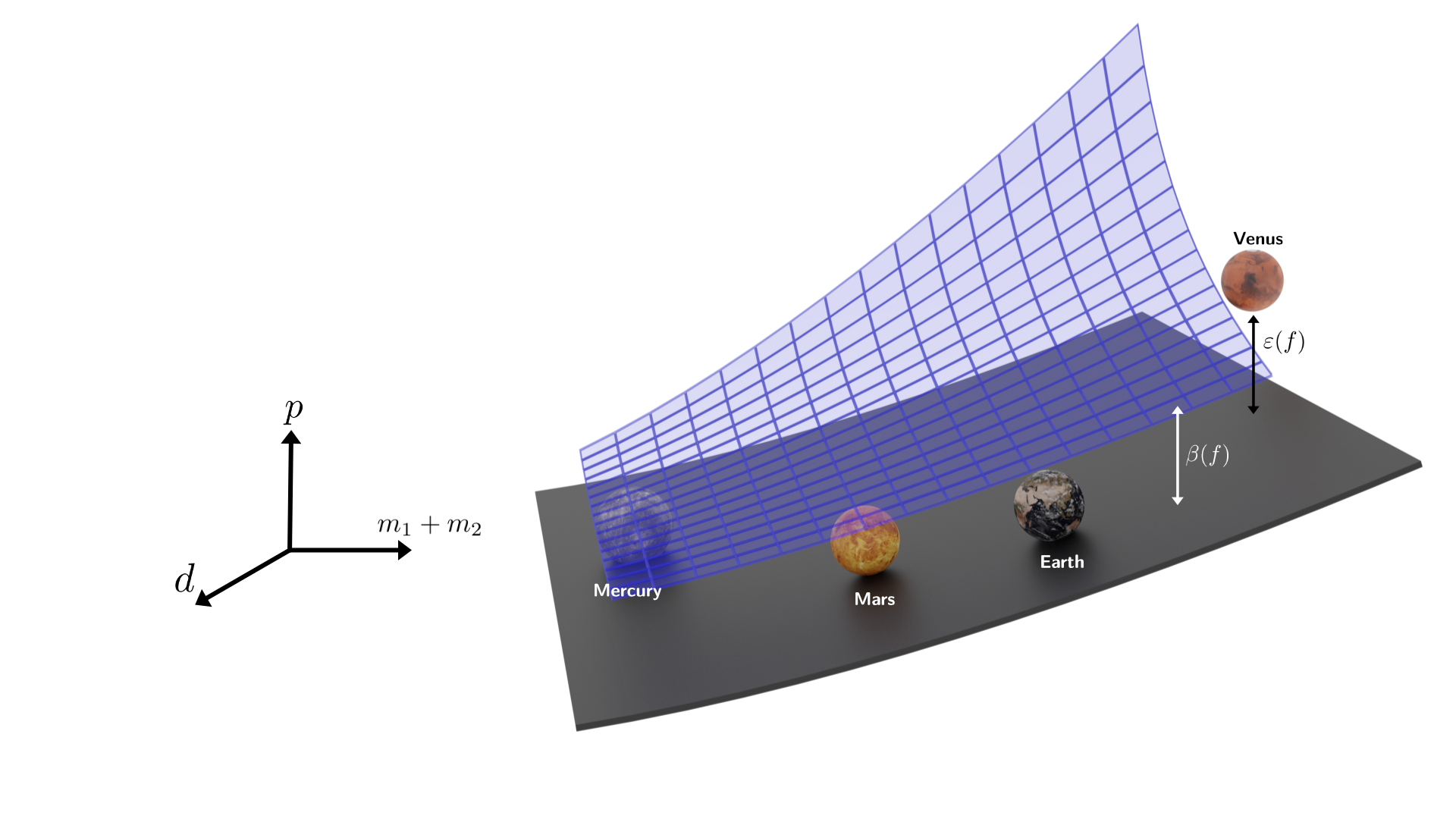
Figure 1: Depiction of the numerical data, background theory, and a discovered model for Kepler’s third law of planetary motion giving the orbital period of a planet in the solar system. The data consists of measurements $(m_{1},m_{2},d,p)$ of the mass of the sun $m_{1}$, the orbital period $p$ and mass $m_{2}$ for each planet and its distance $d$ from the sun. The background theory amounts to Newton’s laws of motion, i.e., the formulae for centrifugal force, gravitational force, and equilibrium conditions. The 4-tuples $(m_{1},m_{2},d,p)$ are projected into $(m_{1}+m_{2},d,p)$. The blue manifold represents solutions of $f_{\mathcal{B}}$ which is the function derivable from the background-theory axioms that represents the variable of interest. The grey manifold represents solutions of the discovered model $f$. The double arrows indicate the distances $\beta(f)$ and $\varepsilon(f)$.

• Background Knowledge  $\mathcal{B}$: a set of domain-specific axioms expressed as logic formulae. They involve $\mathbf{x}$, and $y$, and possibly more variables that are necessary to formulate the background theory. We assume that the background theory $\mathcal{B}$ is complete, that is, it contains all the axioms necessary to comprehensively explain the phenomena under consideration, and consistent, that is, the axioms do not contradict one another. These two assumptions guarantee that there exists a unique derivable function $f_{\mathcal{B}}$ that logically represents the variable of interest $y$.

• A Hypothesis Class  $\mathcal{C}$: a set of admissible symbolic models defined by a grammar, a set of invariance constraints to avoid redundant expressions (e.g., $A+B$ is equivalent to $B+A$) and constraints on the functional form (e.g., monotonicity).

• Data  $\mathcal{D}$: a set of $m$ examples, each providing certain values for $x_{1},\ldots,x_{n}$, and $y$.

• Modeler Preferences  $\mathcal{M}$: a set of numerical parameters, e.g., error bounds on accuracy.

In general, there may not exist a function $f\in\mathcal{C}$ that fits the data exactly and is derivable from $\mathcal{B}$. This could happen because the symbolic model generating the data might not belong to $\mathcal{C}$, the sensors used to collect the data might give noisy measurements, or the background knowledge might be inaccurate or incomplete. To quantify the compatibility of a symbolic model with data and background theory, we introduce the notion of distance between a model $f$ and $\mathcal{B}$. Roughly, it reflects the error between the predictions of $f$ and the predictions of a formula $f_{\mathcal{B}}$ derivable from $\mathcal{B}$ (thus, the distance equals zero when $f$ is derivable from $\mathcal{B}$). Figure 1 provides a visualization of these two notions of distance for the problem of learning Kepler’s third law of planetary motion from solar-system data and background theory.

Our system consists mainly of an SR-module and a reasoning module. The SR-module returns multiple candidate symbolic models (or formulae) expressing $y$ as a function of $x_{1},\ldots,x_{n}$ and that fit the data. For each of these models, the system outputs the distance $\varepsilon(f)$ between $f$ and $\mathcal{D}$ and the distance $\beta(f)$ between $f$ and $\mathcal{B}$. We will also be referring to $\varepsilon(f)$ and $\beta(f)$ as errors.

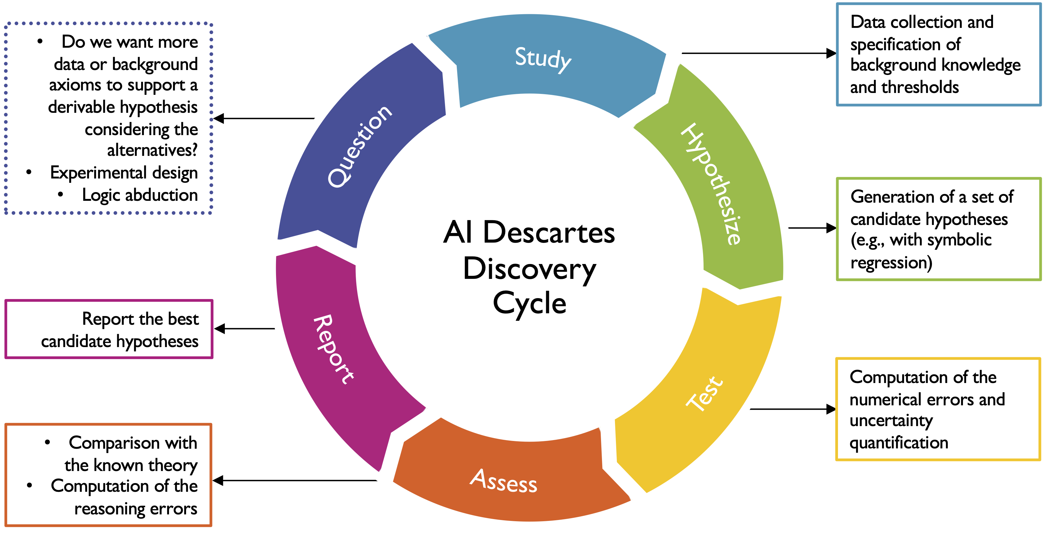
Figure 2: An interpretation of the scientific method as implemented by our system. The colors match the respective components of the system in Fig 3. The box with dotted line boundaries consists of techniques not yet integrated in our system.

These functions are also tested to see if they satisfy the specified constraints on the functional form (in $\mathcal{C}$) and the modeler-specified level of accuracy and complexity (in $\mathcal{M}$). When the models are passed to the reasoning module (along with the background theory $\mathcal{B}$), they are tested for derivability. If a model is found to be derivable from $\mathcal{B}$, it is returned as the chosen model for prediction; otherwise, if the reasoning module concludes that no candidate model is derivable, it is necessary to either collect additional data or add constraints. In this case, the reasoning module will return a quality assessment of the input set of candidate hypotheses based on the distance $\beta$, removing models that do not satisfy the modeler-specified bounds on $\beta$. The distance (or error) $\beta$ is computed between a function (or formula) $f$, derived from numerical data, and the derivable function $f_{\mathcal{B}}$ which is implicitly defined by the set of axioms in $\mathcal{B}$ and is logically represented by the variable of interest $y$. The distance between the function $f_{\mathcal{B}}$ and any other formula $f$ depends only on the background theory and the formula $f$ and not on any particular functional form of $f_{\mathcal{B}}$. Moreover, the reasoning module can prove that a model is not derivable by returning counterexample points that satisfy $\mathcal{B}$ but do not fit the model.

SR is typically solved with genetic programming (GP) [4, 5, 16, 6], however methods based on mixed-integer nonlinear programming (MINLP) have recently been proposed [17, 18, 19]. In this work, we develop a new MINLP-based SR solver (described in the supplementary material). The input consists of a subset of the operators $\{+,-,\times,\div,\sqrt{\ },\log,\exp\}$, an upper bound on expression complexity, and an upper bound on the number of constants used that do not equal $1$. Given a dataset, the system formulates multiple MINLP instances to find an expression that minimizes the least-square error. Each instance is solved approximately, subject to a time limit. Both linear and nonlinear constraints can be imposed. In particular, dimensional consistency is imposed when physical dimensions of variables are available.

We use KeYmaera X [20] as a reasoning tool; it is an ATP for hybrid systems and combines different types of reasoning: deductive, real-algebraic, and computer-algebraic reasoning. We also use Mathematica [21] for certain types of analysis of symbolic expressions. While a formula found by any grammar-based system (such as a SR system) is syntactically correct, it may contradict the axioms of the theory or not be derivable from them. In some cases, a formula may not be derivable as the theory may not have enough axioms; the formula may be provable under an extended axiom set (possibly discovered by abduction) or an alternative one (e.g., using a relativistic set of axioms rather than a “Newtonian” one).

An overview of our system seen as a discovery cycle is shown in Figure 2. Our discovery cycle is inspired by Descartes who advanced the scientific method and emphasized the role that logical deduction, and not empirical evidence alone, plays in forming and validating scientific discoveries. Our present approach differs from implementations of the scientific method that obtain hypotheses from theory and then check them against data; instead we obtain hypotheses from data and assess them against theory.

A more detailed schematic of the system is depicted in Figure 3, where the bold lines and boundaries correspond to the system we present in this work, and the dashed lines and boundaries refer to standard techniques for scientific discovery that we have not yet integrated into our current implementation.

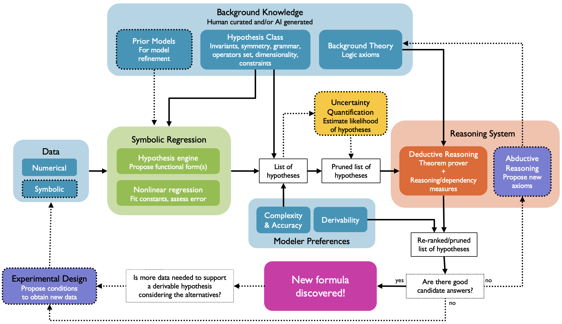
Figure 3: System overview. Solid lines and boundaries correspond to our system, and dotted lines and boundaries indicate standard techniques for scientific discovery (human-driven or artificial) that have not been integrated into the current system. The present system generates hypotheses from data using symbolic regression, which are posed as conjectures to an automated deductive reasoning system, which proves or disproves them based on background theory or provides reasoning-based quality measures.

Results

We tested the different capabilities of our system on three problems (more details in Methods). First, we considered the problem of deriving Kepler’s third law of planetary motion, providing reasoning-based measures to analyze the quality and generalizablity of the generated formulae. Extracting this law from experimental data is challenging, especially when the masses involved are of very different magnitudes. This is the case for the solar system, where the solar mass is much larger than the planetary masses. The reasoning module helps in choosing between different candidate formulae and identifying the one that generalizes well: using our data and theory integration we were able to re-discover Kepler’s third law. We then considered Einstein’s time-dilation formula. Although we did not recover this formula from data, we used the reasoning module to identify the formula that generalizes best. Moreover, analyzing the reasoning errors with two different sets of axioms (one with “Newtonian” assumptions and one relativistic), we were able to identify the theory that better explains the phenomenon. Finally, we considered Langmuir’s adsorption equation, whose background theory contains material-dependent coefficients. By relating these coefficients to the ones in the SR-generated models via existential quantification, we were able to logically prove one of the extracted formulae.

To conclude, we have demonstrated the value of combining logical reasoning with symbolic regression in obtaining meaningful symbolic models of physical phenomena, in the sense that they are consistent with background theory and generalize well in a domain that is significantly larger than the experimental data. The synthesis of regression and reasoning yields better models than can be obtained by SR or logical reasoning alone.

Improvements or replacements of individual system components and introduction of new modules such as abductive reasoning or experimental design (not described in this work for the sake of brevity) would extend the capabilities of the overall system.

A deeper integration of reasoning and regression can help synthesize models that are both data driven and based on first principles, and lead to a revolution in the scientific discovery process. The discovery of models that are consistent with prior knowledge will accelerate scientific discovery, and enable going beyond existing discovery paradigms.

Reproducibility

The code used for this work along with the datasets described below can be found, freely available, at:
https://github.com/IBM/AI-Descartes.

Methods

Kepler’s third law of planetary motion.

Kepler’s law relates the distance $d$ between two bodies, e.g., the sun and a planet in the solar system, and their orbital periods. It can be expressed as

$$p=\sqrt{\frac{4\pi^{2}d^{3}}{G(m_{1}+m_{2})}}\leavevmode\nobreak\ \leavevmode\nobreak\ ,$$ (1)

where $p$ is the period, $G$ is the gravitational constant, and $m_{1}$ and $m_{2}$ are the two masses. It can be derived using the following axioms of the background theory $\mathcal{B}$, describing the center of mass (axiom K1), the distance between bodies (axiom K2), the gravitational force (axiom K3), the centrifugal force (axiom K4), the force balance (axiom K5), and the period (axiom K6):

$$\begin{aligned} \hskip 36.98866pt\text{K1. }&m_{1}*d_{1}=m_{2}*d_{2}\\ \text{K2. }&d=d_{1}+d_{2}\\[4.0pt] \text{K3. }&F_{g}=\frac{Gm_{1}m_{2}}{d^{2}}\\[4.0pt] \text{K4. }&F_{c}=m_{2}d_{2}w^{2}\\[4.0pt] \text{K5. }&F_{g}=F_{c}\\[4.0pt] \text{K6. }&p=\frac{2\pi}{w}\\[4.0pt] \text{K7. }&m_{1}>0,\leavevmode\nobreak\ m_{2}>0,\leavevmode\nobreak\ p>0,\leavevmode\nobreak\ d_{1}>0,\leavevmode\nobreak\ d_{2}>0\leavevmode\nobreak\ \leavevmode\nobreak\ .\end{aligned}$$

We considered three real-world datasets: planets of the solar system, the solar-system planets along with exoplanets from Trappist-1 and the GJ 667 system, and binary stars [22]. These datasets contain measurements of pairs of masses, a sun and a planet for the first two, and two suns for the third, the distance between them, and the orbital period of the planet around its sun in the first two datasets or the orbital period around the common center of mass in the third dataset. The data we use is given in the supplementary material. Note that the dataset does not contain measurements for a number of variables in the axiom system, such as $d_{1},d_{2},F_{g},$ etc. The goal is to recover Kepler’s third law from the data, i.e., to obtain $p$ as the above-stated function of $d$, $m_{1}$ and $m_{2}$. The SR-module takes as input the set $\{+,-,\times,\div,\sqrt{\ }\}$ and outputs a set of candidate formulas.

None of the formulae obtained via SR are derivable, though some are close approximations to derivable formulae. We evaluate the quality of these formulae by writing a logic program for calculating the error $\beta$ of a formula with respect to a derivable formula.

We use three measures, defined below, to assess the correctness of a data-driven formula from a reasoning viewpoint: the pointwise reasoning error, the generalization reasoning error, and variable dependence.

Pointwise reasoning error:

The key idea is to compute a distance between a formula generated from the numerical data and some derivable formula that is implicitly defined by the axiom set. The distance is measured by the $\ell_{2}$ or $\ell_{\infty}$ norm applied to the differences between the values of the numerically-derived formula and a derivable formula at the points in the dataset.

These results can be extended to other norms.

We compute the relative error of numerically derived formula $f(\mathbf{x})$ applied to the $m$ data points $\mathbf{X}^{i}\leavevmode\nobreak\ (i=1,\ldots,m)$ with respect to $f_{\mathcal{B}}(\mathbf{x})$, derivable from the axioms via these expressions:

$$\beta_{2}^{r}=\sqrt{\sum_{i=1}^{m}\left(\frac{f(\mathbf{X}^{i})-f_{\mathcal{B}}(\mathbf{X}^{i})}{f_{\mathcal{B}}(\mathbf{X}^{i})}\right)^{2}}\leavevmode\nobreak\ \leavevmode\nobreak\ \leavevmode\nobreak\ \text{ and }\leavevmode\nobreak\ \leavevmode\nobreak\ \leavevmode\nobreak\ \beta_{\infty}^{r}=\max_{1\leq i\leq m}\left\{\frac{|f(\mathbf{X}^{i})-f_{\mathcal{B}}(\mathbf{X}^{i})|}{|f_{\mathcal{B}}(\mathbf{X}^{i})|}\right\}\leavevmode\nobreak\ .$$ (2)

The KeYmaera formulation of these two measures for the first formula of Table 1 can be found in the supplementary material. Absolute-error variants of the first and second expressions in (2) are denoted by $\beta^{a}_{2},\beta^{a}_{\infty}$, respectively. The numerical (data) error measures $\varepsilon_{2}^{r}$ and $\varepsilon_{\infty}^{r}$ are defined by replacing $f_{\mathcal{B}}(\mathbf{X}^{i})$ by $Y_{i}$ in (2). Analogous to $\beta^{a}_{2}$ and $\beta^{a}_{\infty}$, we also define absolute-numerical-error measures $\varepsilon^{a}_{2}$ and $\varepsilon^{a}_{\infty}$.

Table 1 reports in columns 5 and 6 the values of $\beta_{2}^{r}$ and $\beta_{\infty}^{r}$, respectively. It also reports the relative numerical errors $\varepsilon_{2}^{r}$ and $\varepsilon_{\infty}^{r}$ in columns 3 and 4, measured by the $\ell_{2}$ and $\ell_{\infty}$ norms, respectively, for the candidate expressions given in column 2 when evaluated on the points in the dataset.

The pointwise reasoning errors $\beta_{2}$ and $\beta_{\infty}$ are not very informative if SR yields a low-error candidate expression (measured with respect to the data), and the data itself satisfies the background theory up to a small error, which indeed is the case with the data we use; the reasoning errors and numerical errors are very similar.

Generalization reasoning error:

Even when one can find a function that fits given data points well, it is challenging to obtain a function that generalizes well, i.e., one which yields good results at points of the domain not equal to the data points. Let $\beta^{r}_{\infty,S}$ be calculated for a candidate formula $f(\mathbf{x})$ over a domain $S$ that is not equal to the original set of data points as follows:

$$\beta_{\infty,S}^{r}=\max_{\mathbf{x}\in S}\left\{\frac{|f(\mathbf{x})-f_{\mathcal{B}}(\mathbf{x})|}{|f_{\mathcal{B}}(\mathbf{x})|}\right\}\leavevmode\nobreak\ ,$$ (3)

where we consider the relative error and, as before, the function $f_{\mathcal{B}}(\mathbf{x})$ is not known, but is implicitly defined by the axioms in the background theory. We call this measure the relative generalization reasoning error. If we do not divide by $f_{\mathcal{B}}(\mathbf{x})$ in the above expression, we get the absolute version $\beta_{\infty,S}^{a}$ of this error metric. For the Kepler dataset, we let $S$ be the smallest multi-dimensional interval (or Cartesian product of intervals on the real line) containing all data points. In column 7 of Table 1, we show the relative generalization reasoning error $\beta_{\infty,S}^{r}$ on the Kepler datasets with $S$ defined as above. If this error is roughly the same as $\beta_{\infty}^{r}$ the pointwise relative reasoning error for $\ell_{\infty}$, e.g., for the solar system dataset, then the formula extracted from the numerical data is as accurate at points in $S$ as it is at the data points.

Variable dependence:

In order to check if the functional dependence of a candidate formula on a specific variable is accurate, we compute the generalization error over a domain $S$ where the domain of this variable is extended by an order of magnitude beyond the smallest interval containing the values of the variable in the dataset. Thus we can check whether there exist special conditions under which the formula does not hold. We modify the endpoints of an interval by one order of magnitude, one variable at a time. If we notice an increase in the generalization reasoning error while modifying intervals for one variable, we deem the candidate formula as missing a dependency on that variable. A missing dependency might occur, for example, because the exponent for a variable is incorrect, or that variable is not considered at all when it should be. One can get further insight into the type of dependency by analyzing how the error varies, e.g., linearly or exponentially. Table 1 provides, in columns 8–10, results regarding the candidate formulae for Kepler’s third law. For each formula, the dependencies on $m_{1}$, $m_{2}$, and $d$ are indicated by $1$ or $0$ (for correct or incorrect dependency). For example, the candidate formula $p=\sqrt{0.1319\cdot d^{3}}$ for the solar system does not depend on either mass, and the dependency analysis suggests that the formula approximates well the phenomenon in the solar system, but not for larger masses.

The best formula for the binary-star dataset, $\sqrt{d^{3}/(0.9967m_{1}+m_{2})}$, has no missing dependency (all ones in columns 8–10), i.e., it generalizes well; increasing the domain along any variable does not increase the generalized reasoning error.

Figure 4 provides a visualization of the two errors $\varepsilon^{r}_{2}$ and $\beta^{r}_{2}$ for the first three functions of Table 1 (solar-system dataset) and the ground truth $f^{*}$.

1	2	3	4		5	6		7		8	9	10
	Candidate formula	numerical error			point. reas. err.			gen. reas.		dependencies
Dataset	$p=$	$\varepsilon_{2}^{r}$	$\varepsilon^{r}_{\infty}$		$\beta_{2}^{r}$	$\beta^{r}_{\infty}$		error $\beta^{r}_{\infty,S}$		$m_{1}$	$m_{2}$	$d$
solar	$\sqrt{0.1319d^{3}}$	.01291	.006412		.0146	.0052		.0052		0	0	1
	$\sqrt{0.1316(d^{3}+d)}$	1.9348	1.7498		1.9385	1.7533		1.7559		0	0	0
	$(0.03765d^{3}+d^{2})/(2+d)$	.3102	.2766		.3095	.2758		.2758		0	0	0
exoplanet	$\sqrt{0.1319d^{3}/m_{1}}$	.08446	.08192		.02310	.0052		.0052		0	0	1
	$\sqrt{m_{1}^{2}m_{2}^{3}/d+0.1319\,d^{3}/m_{1}}$	.1988	.1636		.1320	.1097		$>550$		0	0	0
	$\sqrt{(1-.7362m_{1})d^{3}/2}$	1.2246	.4697		1.2418	.4686		.4686		0	0	1
binary stars	$1/(d^{2}m_{1}^{2})+1/(dm_{2}^{2})-m_{1}^{3}m_{2}^{2}\leavevmode\nobreak\ +$	.002291	.001467		.0059	.0050		timeout		0	0	0
	+ $\sqrt{.4787d^{3}/m_{2}+d^{2}m_{2}^{2}}$
	$(\sqrt{d^{3}}+m_{1}^{3}m_{2}/\sqrt{d})/\sqrt{m_{1}+m_{2}}$	.003221	.003071		.0038	.0031		timeout		0	0	0
	$\sqrt{d^{3}/(0.9967m_{1}+m_{2})}$	.005815	.005337		.0014	.0008		.0020		1	1	1

Table 1: Numerical error values, pointwise reasoning error values, and generalization error values for candidate solutions for the Kepler dataset. We also give an analysis of the variable dependence of candidate solutions. For simplicity of notation, in the table we use the variables $d$, $m_{1}$, $m_{2}$ and $p$, while referring to the scaled counterparts. We assume that all the errors are relative.

Figure 4: Depiction of symbolic models for Kepler’s third law of planetary motion giving the orbital period of a planet in the solar system. The model are produced by our SR system by points $(\varepsilon,\beta)$, where $\varepsilon$ represents distance to data, and $\beta$ represents distance to background theory. Both distances are computed with an appropriate norm on the scaled data.

Relativistic time dilation.

Einstein’s theory of relativity postulates that the speed of light is constant, and implies that two observers in relative motion to each other will experience time differently and observe different clock frequencies. The frequency for a clock moving at speed $v$ is related to the frequency ₀ of a stationary clock by the formula

$$\frac{\freq-{}_{0}}{{}_{0}}=\sqrt{1-\frac{v^{2}}{c^{2}}}-1$$ (4)

where $c$ is the speed of light. This formula was recently confirmed experimentally by Chou et al. [23] using high precision atomic clocks. We test our system on the experimental data of [23] which consists of measurements of $v$ and associated values of $(\freq-{}_{0})/{}_{0}$, reproduced in the supplementary material. We take the axioms for derivation of the time dilation formula from  [24, 25]. These are also listed in the supplementary material and involve variables that are not present in the experimental data.

In Table 2 we give some functions obtained by our SR module (using $\{+,-,\times,\div,\sqrt{\ }\,\}$ as the set of input operators) along with the numerical errors of the associated functions and generalization reasoning errors. The sixth column gives the set $S$ as an interval for $v$ for which our reasoning module can verify that the absolute generalization reasoning error of the function in the first column is at most 1. The last column gives the interval for $v$ for which we can verify a relative generalization reasoning error of at most 2%. Even though the last function has low relative error according to this metric, it can be ruled out as a reasonable candidate if one assumes the target function should be continuous (it has a singularity at $v=1$). Thus, even though we cannot obtain the original function, we obtain another which generalizes well, as it yields excellent predictions for a very large range of velocities.

Candidate	Numerical Error		Numerical Error		$S$ s.t. Absolute	$S$ s.t. Relative
formula	Absolute		Relative		Gen. Reas. Error	Gen. Reas. Error
$y=$	$\varepsilon_{2}^{a}$	$\varepsilon^{a}_{\infty}$	$\varepsilon_{2}^{r}$	$\varepsilon^{r}_{\infty}$	$\beta^{a}_{\infty,S}\leq 1$	$\beta^{r}_{\infty,S}\leq 0.02$
$-0.00563v^{2}$	.3822	.3067	1.081	.001824	$37\leq v\leq 115$	$37\leq v\leq 10^{8}$
$\frac{v}{1+0.00689v}-v$	.3152	.2097	1.012	.006927	$37\leq v\leq 49$	$37\leq v\leq 38$
$-0.00537\frac{v^{2}\sqrt{v+v^{2}}}{(v-1)}$	.3027	.2299	1.254	.002147	$37\leq v\leq 98$	$37\leq v\leq 109$
$-0.00545\frac{v^{4}}{\sqrt{v^{2}+v^{-2}}(v-1)}$	.3238	.2531	1.131	.0009792	$37\leq v\leq 126$	$37\leq v\leq 10^{7}$

Table 2: Candidate functions derived from time dilation data, and associated error values. The values of $v$ are defined in $m/s$.

In this case, our system can also help rule out alternative axioms. Consider replacing the axiom that the speed of light is a constant value $c$ by a “Newtonian” assumption that light behaves like other mechanical objects: if emitted from an object with velocity $v$ in a direction perpendicular to the direction of motion of the object, it has velocity $\sqrt{v^{2}+c^{2}}$. Replacing $c$ by $\sqrt{v^{2}+c^{2}}$ (in axiom R2 in the supplementary material to obtain R2’) produces a self-consistent axiom system (as confirmed by the theorem prover), albeit one leading to no time dilation. Our reasoning module concludes that none of the functions in Table 2 is compatible with this updated axiom system: the absolute generalization reasoning error is greater than 1 even on the dataset domain, as well as the pointwise reasoning error. Consequently, the data is used indirectly to discriminate between axiom systems relevant for the phenomenon under study; SR poses only accurate formulae as conjectures.

Langmuir’s adsorption equation.

The Langmuir adsorption equation describes a chemical process in which gas molecules contact a surface, and relates the loading $q$ on the surface to the pressure $p$ of the gas [26]:

$$q=\frac{q_{\mathrm{max}}K_{\mathrm{a}}\cdot p}{1+K_{\mathrm{a}}\cdot p}.$$ (5)

The constants $q_{\mathrm{max}}$ and $K_{a}$ characterize the maximum loading and the adsorption strength, respectively. A similar model for a material with two types of adsorption sites yields:

$$q=\frac{q_{\mathrm{max,1}}K_{\mathrm{a,1}}\cdot p}{1+K_{\mathrm{a,1}}\cdot p}+\frac{q_{\mathrm{max,2}}K_{\mathrm{a,2}}\cdot p}{1+K_{\mathrm{a,2}}\cdot p}\leavevmode\nobreak\ ,$$ (6)

with parameters for maximum loading and adsorption strength on each type of site. The parameters in (5) and (6) fit experimental data using linear or nonlinear regression, and depend on the material, gas, and temperature.

We used data from [26] for methane adsorption on mica at a temperature of 90 K, and also data from [27, Table 1] for isobutane adsorption on silicalite at a temperature of 277 K. In both cases, observed values of $q$ are given for specific values of $p$; the goal is to express $q$ as a function of $p$. We give the SR-module the operators $\{+,-,\times,\div\}$, and obtain the best fitting functions with two and four constants. The code ran for 20 minutes on 45 cores, and seven of these functions are displayed for each dataset.

To encode the background theory, following Langmuir’s original theory [26] we elicited the following set $\mathcal{A}$ of axioms:

L1.	Site balance:	$S_{0}=S+S_{\mathrm{a}}$
L2.	Adsorption rate model:	$r_{\mathrm{ads}}=k_{\mathrm{ads}}\cdot p\cdot S$
L3.	Desorption rate model:	$r_{\mathrm{des}}=k_{\mathrm{des}}\cdot S_{\mathrm{a}}$
L4.	Equilibrium assumption:	$r_{\mathrm{ads}}=r_{\mathrm{des}}$
L5.	Mass balance on $q$	$q=S_{\mathrm{a}}$   .

Here, $S_{0}$ is the total number of sites, of which $S$ are unoccupied and $S_{a}$ are occupied (L1). The adsorption rate $r_{\mathrm{ads}}$ is proportional to the pressure $p$ and the number of unoccupied sites (L2). The desorption rate $r_{\mathrm{des}}$ is proportional to the number of occupied sites (L3). At equilibrium, $r_{\mathrm{ads}}=r_{\mathrm{des}}$ (L4), and the total amount adsorbed, $q$, is the number of occupied sites (L5) because the model assumes each site adsorbs at most one molecule. Langmuir solved these equations to obtain:

$$q=\frac{S_{0}*(k_{\mathrm{ads}}/k_{\mathrm{des}})*p}{1+(k_{\mathrm{ads}}/k_{\mathrm{des}})*p}.$$ (7)

which corresponds to Eq. 5, where $q_{\mathrm{max}}=S_{0}$ and $K_{\mathrm{a}}=k_{\mathrm{ads}}/k_{\mathrm{des}}$. An axiomatic formulation for the multi-site Langmuir expression is described in the supplementary material. Additionally, constants and variables are constrained to be positive, e.g., $S_{0}>0$, $S>0$, and $S_{\mathrm{a}}>0$, or non-negative, e.g., $q\geq 0$.

The logic formulation to prove is:

$$(\mathcal{C}\wedge\mathcal{A})\rightarrow f\leavevmode\nobreak\ ,$$ (8)

where $\mathcal{C}$ is the conjunction of the non-negativity constraints, $\mathcal{A}$ is a conjunction of the axioms, the union of $\mathcal{C}$ and $\mathcal{A}$ constitutes the background theory $\mathcal{B}$, and $f$ is the formula we wish to prove, e.g., (22).

SR can only generate numerical expressions involving the (dependent and independent) variables occurring in the input data, with certain values for constants; for example, the expression $f={p}/{(0.709\cdot p+0.157)}$. The expressions built from variables and constants from the background theory, such as (22), involve the constants (in their symbolic form) explicitly: e.g., $k_{\mathrm{ads}}$ and $k_{\mathrm{des}}$ appear explicitly in (22) while SR only generates a numerical instance of the ratio of these constants. Thus, we cannot use (8) directly to prove formulae generated from SR. Instead, we replace each numerical constant of the formula by a logic variable $c_{i}$ ; for example, the formula $f=p/(0.709\cdot p+0.157)$ is replaced by $f^{\prime}=p/(c_{1}\cdot p+c_{2})$, introducing two new variables $c_{1}$ and $c_{2}$. We then quantify the new variables existentially, and define a new set of non-negativity constraints $\mathcal{C}^{\prime}$. In the example above we will have $\mathcal{C}^{\prime}=c_{1}>0\leavevmode\nobreak\ \wedge\leavevmode\nobreak\ c_{2}>0$.

The final formulation is:

$$\exists c_{1}\cdots\exists c_{n}.\leavevmode\nobreak\ (\mathcal{C}\wedge\mathcal{A})\rightarrow(f^{\prime}\wedge\mathcal{C}^{\prime})\leavevmode\nobreak\ .$$ (9)

For example, $f^{\prime}=p/(c_{1}\cdot p+c_{2})$ is proved true if the reasoner can prove that there exist values of $c_{1}$ and $c_{2}$ such that $f^{\prime}$ satisfies the background theory $\mathcal{A}$ and the constraints $\mathcal{C}$. Here $c_{1}$ and $c_{2}$ can be functions of constants $k_{\mathrm{ads}}$, $k_{\mathrm{des}}$, $S_{0}$, and/or real numbers, but not the variables $q$ and $p$.

We also consider background knowledge in the form of a list of desired properties of the relation between $p$ and $q$, which helps trim the set of candidate formulae. Thus, we define a collection $\mathcal{K}$ of constraints on $f$, where $q=f(p)$, enforcing monotonicity or certain types of limiting behavior (see supplementary material). We use Mathematica [21] to verify that a candidate function satisfies the constraints in $\mathcal{K}$.

1	2	3	4	5	6	7
		Candidate formula	Numerical Error			$\mathcal{K}$
Data	Condition	$q=$	$\varepsilon_{2}^{r}$	$\varepsilon_{\infty}^{r}$	provability	constr.
Langmuir [26, Table IX]	2 const.	$f_{1}:$   $(p^{2}+2p-1)/(.00888p^{2}+.118p)$	.06312	.04865	timeout	2/5
		$f_{2}:$   $p/(.00927p+.0759)$ *	.1799	.1258	Yes	5/5
	4 const.	$f_{3}:$   ${(p^{2}-10.5p-15.)}/{(.00892p^{2}-1.23)}$	.04432	.02951	timeout	2/5
		$f_{4}:$   ${(8.86p+13.9)}/{(.0787p+1)}$	.06578	.04654	No	4/5
		$f_{5}:$   ${p^{2}}/{(.00895p^{2}+.0934p-.0860)}$	.07589	.04959	No	2/5
	4 const.	$f_{6}:$   ${(p^{2}+p)}/{(.00890p^{2}+.106p-.0311)}$	.06833	.04705	timeout	2/5
	extra-point	$f_{7}:$   ${(112p^{2}-p)}/{(p^{2}+10.4p-9.66)}$	.07708	.05324	timeout	3/5
Sun et al. [27, Table 1]	2 const.	$g_{1}:$   ${(p+3)}/{(.584p+4.01)}$	.1625	.1007	No	4/5
		$g_{2}:$   ${p}/{(.709p+.157)}$	.9680	.5120	Yes	5/5
	4 const.	$g_{3}:$   ${(.0298p^{2}+1)}/{(.0185p^{2}+1.16)}-{.000905}/{p^{2}}$	.1053	.05383	timeout	2/5
		$g_{4}:$   ${1}/{(p^{2}+1)}+{(2.53p-1)}/{(1.54p+2.77)}$	.1300	.07247	timeout	3/5
	4 constants	$g_{5}:$   ${(1.74p^{2}+7.61p)}/{(p^{2}+9.29p+0.129)}$	.1119	.0996	timeout	5/5
	extra-point	$g_{6}:$   ${(.226p^{2}+.762p-7.62\cdot 10^{-4})}/{(.131p^{2}+p)}$	.1540	.09348	timeout	2/5
		$g_{7}:$   ${(4.78p^{2}+26.6p)}/{(2.71p^{2}+30.4p+1.)}$	.1239	.1364	timeout	5/5

Table 3: Results on two datasets for the Langmuir problem. (*This expression is also generated when using four constants, and also when an extra point approximating $(0,0)$ is added).

Figure 5: Symbolic regression solutions to two adsorption datasets. $f_{2}$ and $g_{2}$ are equivalent to the single-site Langmuir equation; $g_{5}$ and $g_{7}$ are equivalent to the two-site Langmuir equation.

In Table 3 column 1 gives the data source, and column 2 gives the “hyperparameters" used in our SR experiments: we allow either two or four constants in the derived expressions. Furthermore, as the first constraint C1 from $\mathcal{K}$ can be modeled by simply adding the data point $p=q=0$, we also experiment with an “extra point.” Column 3 displays a derived expression, while the columns 4 and 5 give, respectively, the relative numerical errors $\varepsilon_{2}^{r}$ and $\varepsilon_{\infty}^{r}$. If the expression can be derived from our background theory, then we indicate that in the column 6. These results are visualized in Figure 5. Column 7 indicates the number of constraints from $\mathcal{K}$ that each expression satisfies, verified by Mathematica. Among the top two-constant expressions, $f_{1}$ fits the data better than $f_{2}$, which is derivable from the background theory, whereas $f_{1}$ is not.

When we search for four-constant expressions, we get much smaller errors than (5) or even (6) [26], but we do not obtain the two-site formula (6) as a candidate expression. For the dataset from Sun et al. [27], $g_{2}$ has a form equivalent to Langmuir’s one-site formula, and $g_{5}$ and $g_{7}$ have forms equivalent to Langmuir’s two-site formula, with appropriate values of $q_{\mathrm{max},i}$ and $K_{a,i}$ for $i=1,2$.

System limitations and future improvements

Our results on three problems and associated data are encouraging and provide the foundations of a new approach to automated scientific discovery. However our work is only a first, although crucial, step towards completing the missing links in automating the scientific method.

One limitation of the reasoning component is the assumption of correctness and completeness of the background theory. The incompleteness could be partially solved by the introduction of abductive reasoning [28] (as depicted in Figure 3 of the main paper). Abduction is a logic technique that aims to find explanations of an (or a set of) observation, given a logical theory. The explanation axioms are produced in a way that satisfy the following: 1) the explanation axioms are consistent with the original logical theory and 2) the observation can be deduced by the new enhanced theory (the original logical theory combined with the explanation axioms). In our context the logical theory corresponds to the set of background knowledge axioms that describe a scientific phenomenon, the observation is one of the formulas extracted from the numerical data and the explanations are the missing axioms in the incomplete background theory.

However the availability of background theory axioms in machine readable format for physics and other natural sciences is currently limited. Acquiring axioms could potentially be automated (or partially automated) using knowledge extraction techniques. Extraction from technical books or articles that describe a natural science phenomenon can be done by, for example, deep learning methods (e.g. the work of Pfahler and Morik [29], Alexeeva et al. [30], Wang and Liu [31]) both from NL plain text or semi-structured text such as LateX or HTML. Despite the recent advancements in this research field, the quality of the existing tools remains quite inadequate with respect to the scope of our system.

Another limitation of our system, that heavily depends on the tools used, is the scaling behavior. Excessive computational complexity is a major challenge for automated theorem provers (ATPs): for certain types of logic (including the one that we use), proving a conjecture is undecidable. Deriving models from a logical theory using formal reasoning tools is even more difficult when using complex arithmetic and calculus operators. Moreover, the run-time variance of a theorem prover is very large: the system can at times solve some “large” problems while having difficulties with some smaller problems. Recent developments in the neuro-symbolic area use deep-learning techniques to enhance standard theorem provers (e.g., see Crouse et al. [11]). We are still at the early stages of this research and there is a lot to be done. We envision that the performance and capability (in terms of speed and expressivity) of theorem provers will improve with time. Symbolic regression tools, including the one based on solving mixed-integer nonlinear programs (MINLP) that we developed, often take an excessive amount of time to explore the space of possible symbolic expressions and find one that has low error and expression complexity, especially with noisy data. In practice, the worst-case solution time for MINLP solvers (including BARON) grows exponentially with input data encoding size. See the supplementary material for additional details. However, MINLP solver performance and genetic programming based symbolic regression solvers are active areas of research.

Our proposed system could benefit from other improvements in individual components (especially in the functionality available). For example, Keymaera only supports differential equations in time and not in other variables and does not support higher order logic; BARON cannot handle differential equations.

Beyond improving individual components, our system can be improved by introducing techniques such as experimental design (not described in this work but envisioned in Figure 3 of the main paper[32]). A fundamental question in the holistic view of the discovery process is what data should be collected to give us maximum information regarding the underlying model? The goal of optimal experimental design (OED) is to find an optimal sequence of data acquisition steps such that the uncertainty associated with the inferred parameters, or some predicted quantity derived from them, is minimized with respect to a statistical or information theoretic criterion. In many realistic settings, experimentation may be restricted or costly, providing limited support for any given hypothesis as to the underlying functional form. It is therefore critical at times to incorporate an effective OED framework. In the context of model discovery, a large body of work addresses the question of experimental design for predetermined functional forms, and another body of research addresses the selection of a model (functional form) out of a set of candidates. A framework that can deal with both the functional form and the continuous set of parameters that define the model behavior is obviously desirable [33]; one that consistently accounts for logical derivability or knowledge-oriented considerations [34] would be even better.

Supplementary Material

Datasets

Kepler’s third law of planetary motion

			normalization factors
	Original		Solar	Exoplanet	Binary Stars
$p$	[$s$]		$1000\cdot 24\cdot 60\cdot 60$	$1000\cdot 24\cdot 60\cdot 60$	$365\cdot 24\cdot 60\cdot 60$ [y]
$m_{1}$	[$kg$]		$1.9885\cdot 10^{30}$	$1.9885\cdot 10^{30}$	$1.9885\cdot 10^{30}$
$m_{2}$	[$kg$]		$5.972\cdot 10^{24}$	$1.898\cdot 10^{27}$	$1.9885\cdot 10^{30}$
$d$	[$m$]		$1.496\cdot 10^{11}$ [$au$]	$1.496\cdot 10^{11}$ [$au$]	$1.496\cdot 10^{11}$ [$au$]

Table 4: Units of measurement and normalization factors for Kepler data

We use three different datasets, provided in Table 5. The first has eight data points corresponding to eight planets of the solar system. The second has 20 data points consisting of all eight data points from the first dataset, and, in addition, data points corresponding to some exoplanets in the Trappist-1 and the GJ 667 systems. The third consists of data for five binary stars [22]. All three datasets consist of real measurements of four variables: the distance $d$ between two bodies, a star and an orbiting planet in the first two datasets and binary stars in the third dataset, the masses $m_{1}$ and $m_{2}$ of the two bodies, and the orbital period $p$, which is our target variable. We normalized the data (e.g., masses of planets and stars) to reduce errors that can arise due to processing large numbers in our system. Table 4 gives the original unit of measurement and the normalization factors for each dataset. Each star mass is given as a multiple of the mass of the sun, hence the sun mass equals 1. In the first dataset, each planetary mass is given as a multiple of Earth’s mass, whereas in the second dataset each planetary mass is given relative to Jupiter’s mass. The distance $d$ is given in astronomical units [au]. The period $p$ is given as days$/1000$ or years.

Solar					Exoplanet					Exoplanets (contd.)
$m_{1}$	$m_{2}$	d	t		$m_{1}$	$m_{2}$	d	t		$m_{1}$	$m_{2}$	d	t
1.0	0.0553	0.3870	0.0880		1.0	0.000174	0.3870	0.0880		0.08	0.0043	0.0152	0.0024218
1.0	0.815	0.7233	0.2247		1.0	0.00256	0.7233	0.2247		0.08	0.0013	0.0214	0.0040496
1.0	1.0	1.0	0.3652		1.0	0.00315	1.0	0.3652		0.08	0.002	0.0282	0.0060996
1.0	0.107	1.5234	0.6870		1.0	0.000338	1.5234	0.6870		0.08	0.0021	0.0371	0.0092067
1.0	317.83	5.2045	4.331		1.0	1.0	5.2045	4.331		0.08	0.0042	0.0451	0.0123529
1.0	95.16	9.5822	10.747		1.0	0.299	9.5822	10.747		0.08	0.086	0.063	0.018767
1.0	14.54	19.2012	30.589		1.0	0.0457	19.2012	30.589
1.0	17.15	30.0475	59.800		1.0	0.0540	30.0475	59.800
					0.33	0.018	0.0505	0.0072004
Binary stars					0.33	0.012	0.125	0.02814
0.54	0.50	107.270	1089.0		0.33	0.008	0.213	0.06224
1.33	1.41	38.235	143.1		0.33	0.008	0.156	0.039026
0.88	0.82	113.769	930.0		0.33	0.014	0.549	0.2562
3.06	1.97	131.352	675.5		0.08	0.0027	0.0111	0.0015109

Table 5: Kepler data

Relativistic time dilation

Velocity (m/s)	Time dilation ($10^{-15}$)
0.55	-0.018
4.10	-0.21
8.60	-0.43
14.84	-1.54
22.18	-2.92
29.65	-4.82
36.22	-7.36

Table 6: Time dilation data

We report in Table 6 the data used in [23, Figure 2]. The first column gives the velocity of a moving clock relative to another stationary clock, and the second column gives the relative change in clock rates (i.e., it gives the clock rate (or frequency) of the moving clock minus the clock rate of the stationary clock divided by the clock rate of the stationary clock) scaled by $10^{15}$.

We next list and describe the axioms given as input to the reasoning module for this problem (see Table 7). The period $dt_{0}$ of a “light clock” is defined as the time for light (at velocity $c$) to travel between two stationary mirrors separated by distance $d$ (axiom R1 below). The period $dt$ of a similar pair of mirrors moving with velocity $v$ (axiom R2), is the time taken for light to bounce between the two mirrors, but in this case, while traveling the distance $L$ (calculated via the Pythagorean theorem in axiom R3). The observed change in clock frequency due to motion, $d\freq=\freq-{}_{0}$, (axiom R6) is related to periods $dt_{0}$ and $dt$ using definitions of frequency (axioms A4 and R5). The second column of the previous table gives values for $d\freq/{}_{0}$ (after scaling by $10^{15}$). Here all variables are positive, and the speed of light is taken to be $3\times 10^{8}$ meters per second (axioms R7-R8). In Figure 6, the dashed lines represent lengths, the solid lines represent the direction of travel for light (if vertical or diagonal), or the direction of motion of the light source (horizontal).

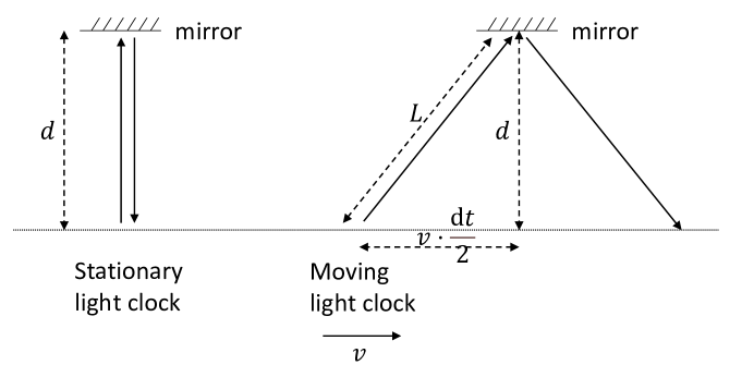
Figure 6: Depiction of moving light clock

R1.	$dt_{0}=2\cdot d/c$				R1’.	$dt_{0}=2\cdot d/c$
R2.	$dt=2\cdot L/c$				R2’.	$dt=2\cdot L/\sqrt{v^{2}+c^{2}}$
R3.	$L^{2}=d^{2}+(v\cdot dt/2)^{2}$				R3.	$L^{2}=d^{2}+(v\cdot dt/2)^{2}$
R4.	${}_{0}=1/dt_{0}$				R4’.	${}_{0}=1/dt_{0}$
R5.	$\freq=1/dt$				R5’.	$\freq=1/dt$
R6.	$d\freq=\freq-{}_{0}$				R6’.	$d\freq=\freq-{}_{0}$
R7.	$d>0,v>0$				R7’.	$d>0,v>0$
R8.	$c=3\times 10^{8}\leavevmode\nobreak\$				R8’.	$c=3\times 10^{8}\leavevmode\nobreak\$

Table 7: Axioms for relativistic time dilation are given in the first two columns, and an alternate set of axioms for “Newtonian behavior” in columns three and four.

Langmuir’s adsorption equation

Data

In Table 8 we provide two datasets, one taken from Langmuir’s original paper [26, Table IX], and the other from [27, Table 1]. Each dataset gives the measured loading $q$ at different values of pressure $p$ at a fixed temperature. We note that different scales for pressure and loading are used in these two datasets.

Langmuir [26, Table IX]			Sun et al. [27, Table 1]
$p$	$q$		$p$	$q$	$p$	$q$
2.7	30.6		0.07	0.695	12.06	1.371
3.7	36.3		0.11	0.752	17.26	1.469
5.2	43.7		0.20	0.797	27.56	1.535
8.0	52.7		0.31	0.825	41.42	1.577
12.8	60.6		0.56	0.860	55.20	1.602
17.3	71.2		0.80	0.882	68.95	1.619
25.8	82.2		1.07	0.904	86.17	1.632
45.0	90.2		1.46	0.923
83.0	98.6		3.51	0.976
122.0	104.0		6.96	1.212

Table 8: Langmuir data

Thermodynamic constraints

A different form of background knowledge is also available for adsorption thermodynamics; axioms for single-component adsorption are more plausible when they satisfy certain thermodynamic constraints $\mathcal{K}$:

C1.	$f(0)=0$
C2.	$(\forall p>0)\leavevmode\nobreak\ (f(p)>0)$
C3.	$(\forall p>0)\leavevmode\nobreak\ (f^{\prime}(p)\geq 0)$
C4.	$0<\lim_{p\rightarrow 0}f^{\prime}(p)<\infty$
C5.	$0<\lim_{p\rightarrow\infty}f(p)<\infty$

C1 requires that at zero pressure, zero molecules may be adsorbed, and C2 requires that only positive loadings are feasible. C3 requires the isotherm increase monotonically with pressure, which holds for all single-component adsorption systems. C4 requires the slope of the adsorption isotherm in the limit of zero pressure (the adsorption second virial coefficient) to be positive and finite [35]. C5 requires the loading to be finite in the limit of infinite pressure, thus imposing a saturation capacity for the material. These five constraints are satisfied by Langmuir and multi-site Langmuir models, but some popular models in the literature violate these to various degrees. For example, Freundlich and Sips formulae violate constraint C4 – a well-known issue critiqued by [35]. The BET isotherm violates C2 and C3 because of its singularity at the vapor pressure of the fluid $p_{\mathrm{vap}}$; this could be resolved by instead enforcing positivity and monotonicity from $0<p<p_{\mathrm{vap}}$.

Additional related work

Symbolic discovery of formulae is a well studied research field, and it is a recognised challenge for the entire Artificial Intelligence community [36].

We addressed the most relevant literature in the introduction to the paper. Some other works worth mentioning are at the intersection of symbolic discovery and deep learning. Several attempts have been made to use deep neural network for learning or discovering symbolic formulae [7, 37, 38, 39, 40, 8, 41]. For example, in the work by Iten et al. [8] the authors focused on modelling a neural network architecture on the human physical reasoning process. In the work by Arabshahi et al. [39] the authors use tree LSTMs to incorporate the structure of the symbolic expression trees, and combine symbolic reasoning and function evaluation for solving the tasks of formula verification and formula completion. Symbolic regression has been used [41] to extract explicit physical relations from components of the learned model of a Graph Neural Network (GNN). In a work by Derner et al. [42], the authors employ symbolic regression to construct parsimonious process models described by analytic formulae for real-time RL control when dealing with unknown or time-varying dynamics. In AI-Feynman [9] (and the subsequent paper AI-Feynman 2.0 [43]), the authors introduce a recursive multidimensional symbolic regression algorithm that combines neural network fitting with a suite of physics-inspired techniques to find an formula that matches data from an unknown function. In the work by Jin et al. [44], symbolic regression is combined with Bayesian models. Moreover, neuro-symbolic systems have received a lot of attention in the past years: see the papers on combining mathematical reasoning with deep neural networks [45, 46]. Bayesian program synthesis has also been successful for learning a library of formulae [47]. Other types of search have been investigated as well, e.g. Bayesian Markov chain Monte Carlo search [48], graph-based search [49], or methods for identifying linear combinations of nonlinear descriptors for dynamic systems (SINDy) [50] or material property prediction (SISSO) [51]. However, to the best of our knowledge, these methods have never been combined with logical reasoning.

The use of logic constraints to help with the discovery of formulas from numerical data is a well known technique.

The LGML tool of Scott et al. 2021 [1], is a pipeline involving a learning component (either a symbolic regression tool or a deep neural network) and a consistency checking component. The consistency checking is performed against a set of equities or inequalities describing the functional form that they are trying to learn: “logical equation in terms of the feature space and the unknown function”. The LGGA tool of Ashok et al. [2] is an extension of LGML and is a genetic algorithm enhanced by auxiliary truth in the form of “mathematical expressions that capture domain specific knowledge or simple properties of an unknown function”. The main goal of the consistency checking component of these two works is to understand if a set of constraints are satisfied by a given function $f^{\prime}$ (the approximation of the correct function $f$). They thus check if $f\textquoteright\models C$. Our work differentiate from these two methods as follows: 1) the type of constraints used is fundamentally different. We use general scientific laws describing the environment, often not including any of the variables present in the data, while in LGML and LGGA they only consider simple constraints on the functional form 2) the reasoning task we are trying to solve is different. As mentioned above LGGA and LGML solve the logic task of $f\textquoteright\models C$ where $f^{\prime}$ is an approximation of the function $f$ and $C$ is a single constraint on $f$ functional form. AI-Descartes solve the task of $B\models f\textquoteright$, where $B$ is a collection of axioms and $f^{\prime}$ is an approximation of the function $f$. Moreover we solve other reasoning tasks such as the computation of the reasoning errors etc. A similar, however earlier, approach is the one by Bladek and Krawiec [52] where the authors formalize the task of symbolic regression with formal constraints by the generation of counterexamples. Another work that combines SR and prior knowledge is the work of Kubalik et al. [3, 53], where the authors consider a set of nonlinear inequality and equality constraints on the functional form of the function to discover. They add this prior knowledge in their multi-objective symbolic regression approach as a set of discrete additional data samples on which candidate models are exactly checked. In this way consistency check can be incorporated into the fitness evaluation or as an additional optimization objective. Finally, the work of Engle and Sahinidis [54] introduce a novel deterministic mixed-integer nonlinear programming formulation for symbolic regression that uses derivative constraints through auxiliary expression trees.

Using logic constraints as part of ML tools increased in popularity in recent years in the Neuro-Symbolic field: e.g. using the violation of logic constraints as part of the loss of an NN[55, 56], or in other techniques [57, 58, 59, 60, 61, 62, 63]. However all these methods are based only on constraints describing the functional form that has to be learnt, and do not incorporate background-theory axioms (logic constraints that describe the other laws and variables that are involved in the phenomenon). Another Neuro-Symbolic research area that is relevant to our work is the extraction of logical rules from data (also called ILP or rule induction). Some examples are the work of Sen et al. [64] or Evans and Grefenstette [65] among many others [66, 67]. A related topic with a lot of attention is program synthesis. Recently there have been a lot of discussion on this topic in the context of Neuro-symbolic systems. Some example are the works of Nye et al. [68], Parisotto et al. [69], Valkov et al. [70] or Yang et al. [71].

Symbolic regression

A symbolic regression scheme consists of a space of valid mathematical expressions composable from a basic list of operators (we assume these to be unary or binary), and a mechanism for exploring the space. Each valid mathematical expression can be represented by an expression tree, i.e., a rooted binary tree where each non-leaf node has an associated binary or unary operator ($+$, $-$, $\times$, $\sqrt{}$, $\log$, etc.), and each leaf node has an associated constant or independent variable. An example of an expression tree for the expression

$$mx^{2}\omega^{2}+\frac{\omega}{mx}$$

is presented in Figure 7 (full expression tree).

Figure 7: Expression tree for $mx^{2}\omega^{2}+\frac{\omega}{mx}$, expressed with full arithmetic notation, and as a more compact tree of L-monomials.

Symbolic regression is often solved with genetic programming (GP). The Eureqa package [72], based on the article [6], is a state-of-the-art GP-based solver. Another popular solver is gplearn [73]. Such solvers search the space of expressions using genetic algorithms. Models generated by GP often suffer from poor accuracy [74] and lengthy descriptions.

The symbolic regression problem can be formulated in various ways as a Mixed-Integer Nonlinear-Programming (MINLP) problem, see [18, 75, 17, 19]. The MINLP problem is solved to global optimality using an off-the-shelf MINLP solver such as BARON [76], COUENNE or SCIP [77]. These solvers solve problems of the form

$$\mathop{\rm Minimize} f(\mathbf{x},\mathbf{y})$$ (10)

s.t. $$g(\mathbf{x},\mathbf{y})\leq\mathbf{b}$$ (11)

$$\mathbf{x}\in\mathbb{R}^{m},\mathbf{y}\in\mathbb{Z}^{m}$$ (12)

where $\mathbf{x}$ is a vector of $m$ continuous variables, $\mathbf{y}$ is a vector of $n$ discrete variables, $f(\mathbf{x},\mathbf{y})$ is a real-valued function that can be composed using a finite list of operators such as $+,-,\times,/,exp(\cdot)$ etc. (this list will vary with each solver), and $g(\mathbf{x},\mathbf{y})$ is a vector-valued function created using the same operators. These solvers use various convex-relaxation schemes to obtain lower bounds on the objective-function value, and utilize these bounds in branch-and-bound schemes to obtain globally optimal solutions.

This approach produces a globally-optimal mathematical expression along with a certificate of optimality, while avoiding an exhaustive search of the solution space. Another advantage is that it directly produces correct, within a tolerance, real-valued constants; most other methods use specialized algorithms to refine constants [78] and cannot guarantee global optimality.

In these MINLPs, the set of valid binary expression trees is specified by a set of constraints over discrete and continuous variables. The discrete variables of the formulation are used to define the structure of the expression tree including the assignment of operators to non-leaf nodes and whether a leaf node is assigned a constant or a specific independent variable. The continuous variables are used for the undetermined constants, and also to evaluate the resulting symbolic expression for specific numerical values associated with individual data points. The objective functions vary from accuracy (measured as sum of squared deviations) to model complexity. The MINLP formulations broadly have the following form:

$$\mathop{\rm Minimize}\leavevmode\nobreak\ \leavevmode\nobreak\ \leavevmode\nobreak\ \leavevmode\nobreak\ \leavevmode\nobreak\ \leavevmode\nobreak\ \mathcal{C}(f_{\theta})$$ complexity

s.t. $$\theta\in\mathcal{T}$$ grammar

$$\mathbf{v}_{i}=f_{\theta}(\mathbf{X}^{(i)}),\leavevmode\nobreak\ \leavevmode\nobreak\ \forall i\in I$$ prediction

$$\mathcal{D}(f_{\theta}(\mathbf{X}),\mathbf{Y})\leq\varepsilon$$ error

where $f_{\theta}$ represents an expression tree defined by the structural and continuous decision variables collectively designated as $\theta$; $\mathcal{T}$ is the universe of valid expression trees; $\mathcal{C}$ measures the description complexity; $\mathcal{D}$ measures error of the predicted values $\mathbf{v}$; $\mathbf{Y}$ is the vector of observations for input vectors $\{\mathbf{X}^{(i)}\}_{i\in I}$.

System Description

We implemented a symbolic regression system based on a novel mixed-integer nonlinear programming formulation. We first describe the basics of our system (without dimensional analysis), and then later explain how we incorporate dimensional analysis.

We take as input a list of operators (for this discussion, assume the input operators are $+,-,\times,/$, and $\sqrt{}$), an upper bound $d$ on the tree depth, an upper bound $k$ on the number of constants, and a domain for the constants $[-\Omega,\Omega]$. In Figure 7, there is a single constant (distinct from 1) with value $1/4$ in the expression tree and in the L-monomial tree. In the prior work on globally optimal symbolic regression, the MINLP formulations typically have discrete variables that (1) determine the placement of the operators in nodes of the expression tree and (2) the mapping of independent variables to leaf nodes, and (3) determine whether to map an independent variable or a constant to a leaf node.

In our formulation, we simply do not have discrete variables for (1). We explicitly enumerate all possible assignments of the operators in expression trees up to depth $d$. More precisely, if a “partial” expression tree is one where the leaf nodes are undetermined, but the operator assignments to non-leaf nodes are determined, then we enumerate all possible partial expression trees up to a certain depth. Our assignment of variables/constants to leaf nodes is also different from prior work. Let $x_{1},\ldots,x_{n}$ be all the independent variables. Instead of assuming that each leaf node is either a constant $h$ or one of $x_{1},\ldots,x_{n}$ as in the prior work, we assume each leaf node is a one-term multivariable Laurent polynomial of the form

$$hx_{1}^{a_{1}}x_{2}^{a_{2}}\cdots x_{n}^{a_{n}},$$ (13)

where $a_{1},\ldots,a_{n}$ are (undetermined) integers (for computational efficiency, we limit these integers to lie in the range $[-\delta,\delta]$ for some input constant $\delta$), and $h$ represents an (undetermined) constant in the final expression. We refer to an expression of the type (13) as an L-monomial. In other words, rather than assigning a single variable or constant to a leaf node, we potentially assign both variables and constants, and also multiple variables (with positive or negative powers to a leaf node). We call the resulting trees generalized expression trees, and gentrees for convenience.

Each gentree $T$ (with depth say $d$) corresponds to a symbolic expression: each non-leaf node with height $1$ corresponds to the expression formed by applying the operator at the node to the expressions (i.e., L-monomials) in the children nodes, and non-leaf nodes at greater heights are handled in the same manner in order of height. The only gentree with depth 0 corresponds to the L-monomial $L_{1}$, whereas the gentrees of depth 1 correspond to the expressions $\sqrt{L_{1}}$, $L_{1}+L_{2}$,  $L_{1}\times L_{2}$,  $L_{1}/L_{2}$ and $L_{1}-L_{2}$, respectively, where $L_{1}$ and $L_{2}$ are L-monomials.

Pruning the list of gentrees

We try to reduce the number of relevant partial expression trees/gentrees by removing a number of "redundant" trees using the fact that the set of nonzero (the constant $h$ in 13 is nonzero) L-monomials is closed under multiplication and division. Notice that both $L_{1}\times L_{2}$ and $L_{1}/L_{2}$ are L-monomials and thus can be represented by a single expression $L_{1}$. In other words, if there is a symbolic expression $f$ of the form $f=L_{1}\times L_{2}$ that fits our data, then there is one of the form $f=L_{1}$. Accordingly our first few pruning rules are: remove a tree $T$ from the list $\mathcal{T}$ of all gentrees with depth up to $d$ if $T$ has the subexpression

[R1] $$L_{1}\times L_{2}\mbox{ or }L_{1}/L_{2}.$$

[R2a] $$L_{1}\times(L_{3}\pm L_{4}).$$

[R2b] $$(L_{1}\pm L_{2})*(L_{3}\pm L_{4}).$$

[R3] $$(L_{1}\pm L_{2})/L_{3}.$$

The first rule was explained above. The second follows by associativity: $L_{1}*(L_{3}+L4)=L_{1}\times L_{3}+L1\times L_{4}=L_{1}^{\prime}+L_{2}^{\prime}$, for some L-monomials $L_{1}^{\prime}$ and $L_{2}^{\prime}$. If a $T$ with a subexpression $L_{1}*(L_{3}+L4)$ appears in $\mathcal{T}$, then replacing this subexpression by $L_{1}^{\prime}+L_{2}^{\prime}$ results in another gentree $T^{\prime}$ of the same depth, which must therefore be in $\mathcal{T}^{\prime}$. The same idea can be applied to the subexpression $L_{1}*(L_{3}-L_{4})$. We can apply associativity twice to justify rule R2b, as $(L_{1}+L_{2})*(L_{3}+L_{4})=L_{1}^{\prime}+L_{2}^{\prime}+L_{3}^{\prime}+L_{4}^{\prime}$, for some $L_{i}^{\prime}$ (the same argument holds when either $+$ is replied by a $-$ in R2b). Once again, the second expression has the same depth as the first, and therefore there must be a tree in $\mathcal{T}$ containing it. R3 can be explained similarly.

MINLP formulation for a gentree

Let the data points be $\mathbf{X}^{(i)}$ for $i\in I$, where $I$ is an index set, and let the features/independent variables be $x_{1},\ldots,x_{n}$. Let $\mathbf{Y}$ stand for the observations of the dependent variable $y$, with $Y^{(i)}$ standing for the $i$-th observation (of the dependent variable). Let $T$ be a given gentree with $m$ leaf nodes, and let $\mathbf{p}$ be the vector of all integer variables corresponding to the powers of the independent variables in the different leaf nodes. Then $\mathbf{p}\in\mathbb{Z}^{mn}$. Let $h_{1},\ldots h_{m}$ be the variables corresponding to the constants in leaf nodes $1,\ldots,m$. Finally, assume we have a 0-1 variable $z_{i}$ that determines whether or not the $i$th leaf node has a constant $h_{i}$ that is different from one. Thus the (vector) variables in our model are $\mathbf{p},\mathbf{z}$ and $\mathbf{h}$. Let $f_{\mathbf{h},\mathbf{p},\mathbf{z},T}$ stand for the symbolic expression defined by fixing the values of these variables. Then the MINLP we solve can be framed as:

$$\min\leavevmode\nobreak\ \leavevmode\nobreak\ \leavevmode\nobreak\ \leavevmode\nobreak\ \leavevmode\nobreak\ \leavevmode\nobreak\ \sum_{i\in I}(Y^{(i)}-f_{\mathbf{h},\mathbf{p},\mathbf{z},T}(\mathbf{X}^{(i}))^{2}$$ (14)

s.t. $$\leavevmode\nobreak\ \leavevmode\nobreak\ \leavevmode\nobreak\ \leavevmode\nobreak\ -\delta\leq p_{i}\leq\delta\leavevmode\nobreak\ \leavevmode\nobreak\ \leavevmode\nobreak\ \mbox{for }i=1,\ldots,mn$$ (15)

$$\leavevmode\nobreak\ \leavevmode\nobreak\ \leavevmode\nobreak\ \leavevmode\nobreak\ -\Omega z_{i}+(1-z_{i})\leq h_{i}\leq\Omega z_{i}+(1-z_{i})\leavevmode\nobreak\ \leavevmode\nobreak\ \leavevmode\nobreak\ \mbox{for }i=1,\ldots,m$$ (16)

$$\leavevmode\nobreak\ \leavevmode\nobreak\ \leavevmode\nobreak\ \leavevmode\nobreak\ \sum_{i=1}^{m}z_{i}\leq k$$ (17)

$$\leavevmode\nobreak\ \leavevmode\nobreak\ \leavevmode\nobreak\ \leavevmode\nobreak\ \mathbf{z}\in\{0,1\}^{m},\leavevmode\nobreak\ \leavevmode\nobreak\ \mathbf{p}\in\mathbb{Z}^{mn}$$ (18)

The constraints (18) and (15) force $z_{i}$ to take on 0-1 values, and $p_{i}$ to take on values in the range $\{-\delta,-\delta+1,\ldots,\delta\}$. The constraint (16) restricts $h_{i}$ to lie in the range $[-\Omega,\Omega]$ if $z_{i}$ has value 1, and forces $h_{i}$ to take on value 1, when $z_{i}$ has value 0. The constraints (17) allow at most $k$ of the $z_{i}$ variables to have value 1, and therefore at most $k$ of the $h_{i}$ values to be different from 1. The function $f_{\mathbf{h},\mathbf{p},\mathbf{z},T}$ is composed of the operators in the non-leaf nodes of $T$ from the L-monomials in the leaf nodes. The objective function is the sum of squares of differences between the symbolic expression values for each input data point and the corresponding dependent variable value (call it the least-square error).

We use BARON to solve the MINLPs we generate, and thus $T$ and $f_{\mathbf{h},\mathbf{p},\mathbf{z},T}$ are limited by the operators that BARON can handle ($+,-,\times,/,\exp(),\log()$). We will illustrate $f$ for a few examples, rather than specify it formally. Suppose we are trying to derive the formula $F=G\,\frac{m_{1}m_{2}}{r^{2}}$, where $m_{1},m_{2}$ and $r$ are independent variables, and $G$ is an unknown constant, and we have multiple data points (for $i\in I$) with values for the independent variables, and for associated $F$. If $T$ is a depth 0 gentree, then $T$ is just a single L-monomial, and $f_{\mathbf{h},\mathbf{p},\mathbf{z},T}=hm_{1}^{a}m_{2}^{b}r_{i}^{c}$ where $a,b,c$ are undetermined integers in the range $[-\delta,\delta]$, and $h$ is an undetermined real number in the range $[-\Omega,\Omega]$. The objective function is then

$$\sum_{i\in I}(F_{i}-hm_{1i}^{a}m_{2i}^{b}r_{i}^{c})^{2}\leavevmode\nobreak\ ,$$

where $F_{i},m_{1i},m_{2i}$ and $r_{i}$ are the values of $F,m_{1},m_{2},r$ in the $i$th data point. If the gentree can be written as $L_{1}+L_{2}$, then the objective function becomes

$$\sum_{i\in I}(F_{i}-(h_{1}m_{1i}^{a_{1}}m_{2i}^{b_{1}}r_{i}^{c_{1}}+h_{2}m_{1i}^{a_{2}}m_{2i}^{b_{2}}r_{i}^{c_{2}}))^{2};$$

here $a_{i},b_{i},c_{i}$ and $h_{i}$ are undetermined, and we solve for these values.

As depicted in Figure 7, an expression tree of a certain depth can sometimes be represented by a gentree of smaller depth. Therefore, by enumerating gentrees of a certain depth, one obtains a much richer class of functions than can be obtained by expression trees of the same depth.

Enumeration and parallel processing

By enumerating the generalized expression trees and solving them separately, the problem is divided into multiple, easier-to-solve sub-problems (operator placement in non-leaf nodes does not have to be determined any more) that can be solved much more quickly. This "divide and conquer" formulation can obtain solutions to problems that were intractable for the formulation in [17].

When available, we exploit parallelism, and run multiple threads, with one MINLP corresponding to a single gentree in a single thread. If we obtain a solution that fits the data within a prescribed tolerance from a gentree with depth $d^{\prime}$, then we stop all processes/threads containing gentrees with depth $>d^{\prime}$. We terminate a gentree if the lower bound on the least-square error exceeds the least-square error found from other gentrees of the same or lower depth. Thus we execute a branch-and-bound type search, and implicitly search for the least depth gentree that fits the data.

If we have more gentrees than available cores, we process them in a round robin fashion; if $t$ is the number of cores, we start solving for $t$ gentrees in parallel, and after a fixed amount of time (10 seconds), we pause the first $t$ gentrees, and start solving $t$ more, till we either find a solution or run out of gentrees in which we case we start from the first gentree. The gentrees are sorted by a measure of complexity (roughly equal to the number of nodes).

Scaling

The gentree enumeration running time (and thus that of our overall algorithm) grows exponentially with gentree depth $d^{\prime}$. As described earlier, we enumerate a number of gentrees, and solve an MINLP per gentree. The number of distinct gentrees grows exponentially with the depth $d^{\prime}$ of the gentree and also grows rapidly with the number of operators used; see Table 9.

	Number of trees with	Number of trees with
Max tree depth	operators: $+$, $-$, $\times$, $/$	operators: $+$, $-$, $\times$, $/$, $\sqrt{}$
1	2	2
2	6	7
3	31	60
4	1153	4485
5	1,506,165	$\geq$ 10,000,000

Table 9: Number of gentrees as a function of depth

The number of gentrees for $d^{\prime}=2,3,4,5$ are, respectively, 7, 60, 4485 and over ten million when we use the operators $+$, $-$, $\times$, $/$, $\sqrt{}$. Our gentree enumeration approach is unlikely to be tractable for $d^{\prime}\geq 6$ and is already hard for $d^{\prime}=4$ if we include more operators than listed earlier. But each L-monomial can represent large expression trees. The L-monomial $hm_{1}^{a}m_{2}^{b}r_{i}^{c}$, which corresponds to a depth 0 gentree, needs a depth 3 binary expression tree if the powers $a,b,c$ are integers between $-2$ and $2$. Thus our depth-3 L-monomial trees can easily need expression trees with depth 6 or more to represent them when we have three independent variables. If the number of independent variables in the L-monomial is more than 3, or the magnitude of the powers is increased, then even deeper expression trees would be needed.

Solving the MINLP problem associated with each gentree can itself be a hard problem. MINLP solvers such as BARON typically use a branch-and-bound algorithm to solve such a problem to a prescribed tolerance. Upon termination (assuming a minimization problem) BARON returns both a solution and a lower bound on all possible solution objective values such that the returned solution objective value and the lower bound differ by less than the prescribed tolerance. However, the number of branch-and-bound nodes – and the computing time – can grow exponentially. To avoid exponential growth, we terminate the process within a prescribed time limit and end up with a large gap between the objective value and the lower bound. In Figures 8 and 9, we show how the upper bound (on the absolute error between the derived model and data) and lower bound change with time during the MINLP solution process along with the growth in number of branch-and-bound nodes. In the first figure we observe that shortly after 500 seconds, BARON certifies that the optimal error is roughly 8.5. In the second figure we observe that the error drops to roughly 0.002 shortly before 300 seconds, but the process does not terminate as BARON is unable to improve the lower bound from 0 (and termination conditions are either the absolute gap between bounds should be $10^{-4}$ or the relative gap between bounds should be $10^{-3}$). Consider the single MINLP associated with the gentree in Figure 9, and assume we have 3 independent variables and the powers of each variable are constrained to be integers between 2 and -2 (see the later section on our experimental settings). The number of possible discrete choices to be made (i.e., the power of each variable in each L-monomial) is at least $5^{15}\approx 30$ billion. BARON is able to obtain a solution of reasonable quality by examining about 120,000 subproblems.

Figure 8: (a) Change with time in upper bound and lower bound values for the MINLP associated with the gentree for $L_{1}+L_{2}+L_{3}$; (b) Growth in number of branch-and-bound nodes with time.

Figure 9: (a) Change with time in upper bound for the MINLP associated with the gentree $\big{(}\sqrt{(L_{1}+L_{2})}\cdot(L_{3}+L_{4})\big{)}/L_{5}$ (the lower bound remains zero throughout); (b) Growth in number of branch-and-bound nodes with time.

Dimensional analysis

Consider Newton’s law of universal gravitation which says that the gravitational force between two bodies is proportional to the product of their masses and inversely proportional to the square of the distance between their centers (of gravity):

$$F\propto\frac{m_{1}m_{2}}{r^{2}}$$

and the constant of proportionality is G, the gravitational constant. Therefore, we have

$$F=G\,\frac{m_{1}m_{2}}{r^{2}}.$$

The units of $G$ are chosen so that units of the right-hand-side expression equal the units of force (mass $\times$ distance $/$ time-squared). Suppose one is given a data set for this example, where each data item has the masses of two bodies and the distance and gravitational force between them. Dimensional analysis would rule out $F=m_{1}m_{2}/r^{2}$ or $F=m_{1}/m_{2}+m_{2}r$, for example, as possible solutions.

If constants can have units and every L-monomial can have a such a constant, then dimensional analysis conveys essentially no information. For example, we can choose constants $h_{1},h_{2},h_{3}$ with appropriate dimensions so that both the expressions $F=h_{1}m_{1}m_{2}/r^{2}$ and $F=h_{2}m_{1}/m_{2}+h_{3}m_{2}r$ satisfy all dimensional requirements. We allow constants to have units or not based on an input flag.

We next explain the constraints we add to our formulation to enforce dimensional consistency. Assume that all constants have no units, and that $k=2$, and $\delta=2$, and $d=1$. For the gravitation example (without the gravitational constant $G$ as an input), each L-monomial $L$ has the form

$$L=hm_{1}^{a}m_{1}^{b}r^{c},$$ (19)

where $a$, $b$ and $c$ are bounded integer variables with an input range of $[-2,2]$, and $h$ is a variable representing a constant. We add to the system of constraints (15) - (18) linear constraints that equate the units of the symbolic expression to those of the dependent variable. For the case our gentree consists of a single node (as in the first tree in Figure 1), our symbolic expression has the form (19), and we add the linear constraints

$$a\left[\begin{matrix}1\\ 0\\ 0\end{matrix}\right]+b\left[\begin{matrix}1\\ 0\\ 0\end{matrix}\right]+c\left[\begin{matrix}0\\ 1\\ 0\end{matrix}\right]=\left[\begin{matrix}\leavevmode\nobreak\ \leavevmode\nobreak\ \leavevmode\nobreak\ 1\\ \leavevmode\nobreak\ \leavevmode\nobreak\ \leavevmode\nobreak\ 1\\ -2\end{matrix}\right]\leavevmode\nobreak\ .$$

Here, each component of a column vector corresponds to a unit (mass, distance, time, respectively). The column on the right-hand side represents the units of force, i.e., mass times distance divided by squared time. The columns on the left-hand side represent the dimensionalities of mass and distance, respectively. The third of the above linear equations does not have a solution.

Next, assume the symbolic expression is $L_{1}+L_{2}$ where $L_{1}=h_{1}m_{1}^{a_{1}}m_{2}^{b_{1}}r^{c_{1}}$ and $L_{2}=m_{1}^{a_{2}}m_{2}^{b_{2}}r^{c_{2}}$, and the unkowns are $a_{i},b_{i},c_{i}$ and $h_{i}$. The units of $L_{1}$ and $L_{2}$ have to match, and must also equal the units of $F$. The linear constraints we add are

$$a_{1}\left[\begin{matrix}1\\ 0\\ 0\end{matrix}\right]+b_{1}\left[\begin{matrix}1\\ 0\\ 0\end{matrix}\right]+c_{1}\left[\begin{matrix}0\\ 1\\ 0\end{matrix}\right] =\left[\begin{matrix}\leavevmode\nobreak\ \leavevmode\nobreak\ \leavevmode\nobreak\ 1\\ \leavevmode\nobreak\ \leavevmode\nobreak\ \leavevmode\nobreak\ 1\\ -2\end{matrix}\right]$$ (20)

$$a_{2}\left[\begin{matrix}1\\ 0\\ 0\end{matrix}\right]+b_{2}\left[\begin{matrix}1\\ 0\\ 0\end{matrix}\right]+c_{2}\left[\begin{matrix}0\\ 1\\ 0\end{matrix}\right] =\left[\begin{matrix}\leavevmode\nobreak\ \leavevmode\nobreak\ \leavevmode\nobreak\ 1\\ \leavevmode\nobreak\ \leavevmode\nobreak\ \leavevmode\nobreak\ 1\\ -2\end{matrix}\right].$$ (21)

Finally, for the symbolic expression $L_{1}\times L_{2}$, to compute the units of this expression we need to add up the units of $L_{1}$ and of $L_{2}$. Thus we sum the left hand sides of (20) and (21) and equate this sum to the right hand side of (20). We can similarly deal with dimension matching in the remaining gentrees of depth 1 via linear constraints. For greater depth gentrees, we apply the ideas above to depth 1 (non-leaf nodes), and then to depth 2 nodes and so on.

Settings for experiments

Because of the exponential worst-case scaling behavior of our method, we choose specific parameters that allow our method to terminate in a reasonable amount of time.

We set the depth limit $d$ to 3. We experiment with different values of $k$, the number of constants, for each dataset. We terminate when we find an expression with objective value (squared error) less than $10^{-4}$ (error tolerance). The operators we use are described in Section System Description of Symbolic Regression. We set $\Omega$ to 100, so all constants are in the range $[-100,100]$. We set $\delta=2$ for computational efficiency. This means that each power in an L-monomial lies in the range $[-2,2]$. Under this setting, the pruning rules – R1, R2,R3 – remove potentially non-redundant gentrees, and our algorithm does not explore all possible symbolic expressions that are representable as a gentree of depth up to 3. Though L-monomials are closed under multiplication, L-monomials with bounded powers are not. For example, if there is a solution of the form $x_{1}^{3}x_{2}^{2}$, we may not find it.

We constrain the search in three more ways. We bound the sum of the variable powers in an L-monomial by an input number $\tau=6$. Thus, for each term of the type (13), we add the constraint $\sum_{i=1}^{n}|a_{i}|\leq\tau$, which is representable by a linear constraint using $n$ auxiliary variables $a_{i}^{\prime}:\sum_{i=1}^{n}a_{i}^{\prime}\leq\tau$ and $a_{i}^{\prime}\geq 0,-a_{i}\leq a_{i}^{\prime}$ and $a_{i}\leq a_{i}^{\prime}$ for $i=1,\ldots,n$. Secondly, we add another pruning rule. We remove any gentree which contains a subexpression of the form $\sqrt{L}$ where $L$ is an L-monomial (we allow $\sqrt{L_{1}+L_{2}}$, for example). We use dimensional analysis when feasible, other than when we perform a comparison with other SR codes (for example in Tables LABEL:tab:ai-feynman-results - 18) which do not use dimensional analysis.

Reasoning and Derivability

Logic and Reasoning Background

We assume the reader has knowledge of basic first-order logic and automated theorem proving terminology and thus will only briefly describe the terms commonly seen throughout this paper. For readers interested in learning more about logical formalisms and techniques see [79, 80].

In this work, we focus on first-order logic (FOL) with equality and basic arithmetic operators. In the standard FOL problem-solving setting, an Automated Theorem Prover (ATP), also called a reasoner, is given a conjecture, that is, a formula to be proved true or false, and axioms, that is, formulae known to be true. The set of axioms is also called the background theory. By application of an inference rule, a new true formula can be derived from the axioms. This operation can be repeated, including the use of prior derived formulae; this yields a sequence of new true formulae, called a derivation. This is done until the given conjecture appears among the derived formulae; the sequence of applied rules and formulae along the way comprise a proof of the given conjecture. The set of all derivable formulae from a background theory is the set of all logic formulae that can be derived from the set of axioms defining the background theory.

All formulae considered in this work are FOL formulae with equality and basic arithmetic operators, and so are defined based on the FOL grammar with the addition of the function symbols for equality $=$, inequality $>,\leavevmode\nobreak\ <$, sum $+$, subtraction $-$, product $*$, division $/$, power ^ (the square root is interpreted as a power of $\frac{1}{2}$) and absolute value $|\cdot|$.

First-order logic formulae are formal expressions based on an alphabet of predicates, functions, and variable symbols which are combined by logical connectives. A term is either a variable, a constant (function with no arguments), or, inductively, a function applied to a tuple of terms. A formula is either a predicate applied to a tuple of terms or, inductively, a connective (e.g., $\wedge$ read as “and”, $\vee$ as “or”, $\neg$ as negation, etc.) applied to some number of formulae. In addition, variables in formulae can be universally or existentially quantified (i.e., by the quantifiers $\forall$ and $\exists$ which read as “for all” and “exists” respectively), where a quantifier introduces a semantic restriction for the interpretation of the variables it quantifies.

KeYmaeraX

Reasoning software tools for arithmetic and calculus that, in principle, have the required logic capabilities of checking consistency, validation, and deduction include: SymPy [81], Prolog [82], Mathematica [21], Beagle [83], and KeYmaera [20, 84].

We integrated in our system several reasoning tools for arithmetic and calculus, analyzing their expressiveness and capabilities (including, but not only, the one mentioned above). Our findings made us decide in favour of the KeYmaeraX reasoner, an automated theorem prover for hybrid systems that combines different types of reasoning: deductive, real algebraic, and computer algebraic reasoning. The underlying logic supported by KeYmaera is differential dynamic logic [85], which is a real-valued first-order dynamic logic for hybrid programs. KeYmaera is based on a generalized free-variable sequent calculus inference rule for deductive reasoning and has an underlying CAD system (e.g. Mathematica).

KeYmaeraX provides fast computation for first-order logical formulae combined with arithmetic and differential equations, even though it does not provide full explainability for the derivations, meaning that only the final state (provable/not-provable) is available, while the proof-steps are not.

KeYmaeraX formulation for Kepler’s third law

We first consider the KeYmaera formulation for the $\beta^{r}_{\infty}$ error. As an example, we consider $f(\mathbf{x})$ corresponding to $p=\sqrt{0.1319\cdot d^{3}}$ extracted via SR from the solar system dataset. We compute the error between this function and $f_{\mathcal{B}}$, represented by $\mathtt{p}$, which is the variable corresponding to the orbital period.

⬇

1Problem (( m1>0 & m2>0 & p>0 & d2>0 & d1>0 & m1N>0 & m2N>0 & pN>0

2 & G = (6.674 * 10^(-11)) & pi = (3.14) & err = 10^-2

3 & ( m1 * d1 = m2 * d2 )

4 & ( d = d1 + d2 )

5 & ( Fg = (G * m1 * m2) / d^2 )

6 & ( Fc = m2 * d2 * w^2 )

7 & ( Fg = Fc )

8 & ( p = (2 * pi )/w )

9 & convP = (1000 * 24 * 60 * 60 )

10 & convm1 = (1.9885 * 10^30 )

11 & convm2 = (5.972 * 10^24)

12 & convD = (1.496 * 10^11)

13 & m1N = m1 / convm1

14 & m2N = m2 / convm2

15 & dN = d / convD

16 & pN = p / convP

17 )->(((m1N=1 & m2N=0.055 & dN=0.3871) ->

18 abs((0.1319 * dN^3 )^(1/2) - (pN))/pN < err)

19 & ((m1N=1 & m2N=0.815 & dN=0.7233) ->

20 abs((0.1319 * dN^3 )^(1/2) - (pN))/pN < err)

21 & ((m1N=1 & m2N=1 & dN=1) ->

22 abs((0.1319 * dN^3 )^(1/2) - (pN))/pN < err)

23 & ((m1N=1 & m2N=0.107 & dN=1.5237) ->

24 abs((0.1319 * dN^3 )^(1/2) - (pN))/pN < err)

25 & ((m1N=1 & m2N=317.8 & dN=5.2044) ->

26 abs((0.1319 * dN^3 )^(1/2) - (pN))/pN < err)

27 & ((m1N=1 & m2N=95.159 & dN=9.5826) ->

28 abs((0.1319 * dN^3 )^(1/2) - (pN))/pN < err)

29 & ((m1N=1 & m2N=14.536 & dN=19.2184) ->

30 abs((0.1319 * dN^3 )^(1/2) - (pN))/pN < err)

31 & ((m1N=1 & m2N=17.147 & dN=30.07) ->

32 abs((0.1319 * dN^3 )^(1/2) - (pN))/pN < err)

33) ) End.

In particular we see that:

• line 1 describes the feasibility constraints, e.g., the masses only admit positive values;

• line 2 defines some constants such as the gravitational constant, the value of $\pi$ ($\mathtt{pi}$), and the error bound ($\mathtt{err}=10^{-2}$ );

• lines 3-8 are the axioms of the background theory;

• lines 9-16 are the normalization specifications (e.g. $\mathtt{m1N}$ is the normalized variable corresponding to the mass $\mathtt{m_{1}}$);

• lines 17-24 contain the specification of the $\beta^{r}_{\infty}$ error: given each data point, which specifies the value of the two masses and their relative distance, we want to prove that the distance between the formula induced from the data (in this case $p=\sqrt{0.1319\cdot d^{3}}$) and the actual formula derivable from the axioms for $p$ is smaller than the value of $\mathtt{err}$. In this way, if all the data points respect the error bound, the $\max$ value will as well.

KeYmaera is able to produce a successful proof of the formulation above for an error bound of $\mathtt{err}=10^{-2}$.

The value for the reasoning error $\beta^{r}_{\infty}$ is computed by using binary search over the values of the relative error $|(\sqrt{0.1319*d^{3}}-p)|/p$. In these experiments we used a time limit of $1200$ seconds (20 min) and stopped the binary search process when a precision of $10^{-4}$ is attained.

The formulation for $\beta^{r}_{2}$ error is very similar, with the difference that the binary search is performed over the single data points as described in Algorithm 1, where

$$\min_{e}{\{\textrm{KeYmaera}\ell_{2}(i,e)\mid\texttt{precision}\}}$$

computes an upperbound on the minimum value for $e$ for a give precision level (which is $10^{-4}$ in the experiments) such that $\textrm{KeYmaera}\ell_{2}(i,e)$ returns $true$. This is necessary because KeYmaera is fundamentally a boolean function, mapping formulations to a success/failure state and is thus not able to perform optimization over continuous values. The minimum is therefore calculated approximately (via binary search) in a given interval with an input precision level and fixing a time limit (20 min in the experiments).

Algorithm 1 $\beta^{r}_{2}$ computed with KeYmaera

1:procedure $\beta^{r}_{2}$(Dataset)

2:     for $i$ in Dataset do

3:         $e_{i}\leftarrow\min_{e}{\{\textrm{KeYmaera}\ell_{2}(i,e)\mid\texttt{precision}\}}$      

4:     $\beta^{r}_{2}\leftarrow\sqrt{e_{i}^{2}+\cdots+e_{n}^{2}}$

5:return $\beta^{r}_{2}$

The KeYmaera formulation for $\textrm{KeYmaera}\ell_{2}(i,e)$ on a specific data point $i$ and an error bound $e$ is a Boolean function that returns $true$ if the following program is provable and $false$ otherwise. $\textrm{KeYmaera}\ell_{2}(i,e)$ returns $true$ when, for a given set of axioms, the absolute value of the relative distance between a given function and a derivable one is smaller than $e$ for a given data point $i$. For example, given the data point $(m_{1},m_{2},d)=(1,0.055,0.3871)$ and error $e=10^{-2}$ we have the following formulation:

⬇

1Problem (( m1>0 & m2>0 & p>0 & d2>0 & d1>0 & m1N>0 & m2N>0 & pN>0

2 & G = (6.674 * 10^(-11)) & pi = (3.14) & e = 10^-2

3 & ( m1 * d1 = m2 * d2 )

4 & ( d = d1 + d2 )

5 & ( Fg = (G * m1 * m2) / d^2 )

6 & ( Fc = m2 * d2 * w^2 )

7 & ( Fg = Fc )

8 & ( p = (2 * pi )/w )

9 & convP = (1000 * 24 * 60 * 60 )

10 & convm1 = (1.9885 * 10^30 )

11 & convm2 = (5.972 * 10^24)

12 & convD = (1.496 * 10^11)

13 & m1N = m1 / convm1

14 & m2N = m2 / convm2

15 & dN = d / convD

16 & pN = p / convP

17 )->(((m1N=1 & m2N=0.055 & dN=0.3871) ->

18 abs((0.1319 * dN^3 )^(1/2) - (pN))/pN < e)

19) ) End.

We observed that the point-wise reasoning errors are not very informative if SR yields a low-error candidate expression (measured with respect to the data), and the data itself satisfies the background theory up to a small error, which indeed is the case with the data we use; the reasoning errors and numerical errors are very similar. This is true because if we can evaluate the numerical error, i.e., we have data for the real values of $p$, then we may assume that the error of the candidate formula at the data points is substantially equal to the error of the correct formula. In particular, this is true when the data is generated synthetically like in [9].

However, this analysis is still relevant if we wish to evaluate the error in the data:

$$\textit{Error in the data }=\textit{ Numerical error }-\textit{ Reasoning error}\leavevmode\nobreak\ .$$

The latter is useful for avoiding overfitting entailed in formulae with numerical error smaller than error in the data.

Let’s consider again the formula $\sqrt{0.1319\cdot d^{3}}$ (extracted via SR from the solar system dataset) for the variable of interest $p$. The KeYmaera formulation for the generalization relative reasoning error $\beta^{r}_{\infty,S}$ is the following:

⬇

1Problem (( p>0 & pN>0

2 & G = (6.674 * 10^(-11)) & pi = (3.14) & err = 10^-6

3 & m1N>=0.08 & m1N<=1

4 & m2N>=0.0002 & m2N<=1

5 & dN>=0.0111 & dN<=30.1104

6 & ( m1 * d1 = m2 * d2 )

7 & ( d = d1 + d2 )

8 & ( Fg = (G * m1 * m2) / d^2 )

9 & ( Fc = m2 * d2 * w^2 )

10 & ( Fg = Fc )

11 & ( p = (2 * pi )/w )

12 & convP = (1000 * 24 * 60 * 60 )

13 & convm1 = (1.9885 * 10^30 )

14 & convm2 = (5.972 * 10^24)

15 & convD = (1.496 * 10^11)

16 & m1N = m1 / convm1

17 & m2N = m2 / convm2

18 & dN = d / convD

19 & pN = p / convP

20 )->((abs(0.1319 * dN^3 )^(1/2) - pN ) / (pN) < err ))

21End.

In particular we have that:

• line 1 describes the feasibility constraints;

• line 2 defines some constants such as the gravitational constant, $\pi$ value and the error bound;

• lines 3-5 define the intervals $S$ for the variables, extracted from the dataset normalized data points (e.g. the planets in the solar system have a distance more than $0.0111$ astronomical units and less than $30.1104$ astronomical units from the sun);

• lines 6-11 are the axioms of the background theory;

• lines 12-19 are the normalization specifications;

• lines 17-24 contain the specification of the error $\beta^{r}_{\infty,S}$: given each data point (instantiation of the value of the two masses and their relative distance) we want to prove that the distance between the formula induced from the data (in this case $\sqrt{0.1319\cdot d^{3}}$) and the actual formula derivable from the axioms for $p$ is smaller than the value of $\mathtt{err}$.

KeYmaera formulation for relativistic time dilation

We give a formulation to check for the quality of generalization for a given formula, in particular, the function $y=-0.00563v^{2}$ computed from data. The velocity of light $c$ is given as a fixed constant 3 $\times 10^{8}$ (meters per second). The generalized absolute reasoning error $\beta^{a}_{\infty,S}$ is bounded above by $1$. The following formulation checks if all the derivable formulae differs (after scaling by $10^{15}$) from the function $-0.00563v^{2}$ by at most $1$ in the domain $S$ defined by $37\leq v\leq 115$.

⬇

1Problem((d > 0 & L > 0 & c = 3*10^8 & err = 1

2 & v >= 37 & v <= 115

3 & dt0 = 2*d/c

4 & L^2 = d^2 + (v*dt/2)^2

5 & dt = 2*L/c

6 & f0 = 1/dt0

7 & f = 1/dt

8 & df = f - f0

9 & y = 10^15*df/f0 )

10 -> ( ( abs( (-0.00563)*(v^2)) - y < err ) ) )

11End.

KeYmaeraX formulation for proving Langmuir’s adsorption equation

The KeYmaeraX formulation to prove the Langmuir equation:

$$q=\frac{S_{0}\cdot(k_{\mathrm{ads}}/k_{\mathrm{des}})\cdot p}{1+(k_{\mathrm{ads}}/k_{\mathrm{des}})\cdot p}.$$ (22)

from the background theory described in the manuscript (L1–L5) is the following:

⬇

1Definitions

2 Real kads;

3 Real kdes;

4 Real S0;

5End.

6Problem

7( \forall Q \forall S \forall Sa \forall P \forall rdes \forall rads(

8 (kads>0 & kdes>0 & S0>0 & Q>0 & S>0 & Sa>0 & P>0 & rdes>0 & rads>0

9 & S0 = S + Sa

10 & rads = kads * P * S

11 & rdes = kdes * Sa

12 & rads = rdes

13 & Q = Sa)

14 -> Q = ((S0 * (kads / kdes)) * P) / (1 + ((kads / kdes)*P) ) ))

15End.

This formulation is successfully proved by KeYmaera.

As expected, when removing one or more axioms that are strictly necessary to prove the theorem (e.g., the axiom $r_{\mathrm{des}}=k_{\mathrm{des}}\cdot S_{\mathrm{a}}$), it is not possible to prove the formula anymore. Similarly, if $f$ does not correspond to the correct formula (while the axiom set is complete and correct) KeYmaera is not able to provide a provability certification. In this case it is possible to create a numerical counterexample (a numerical assignment to all the variables involved in the problem formalization, that falsify the implication). Moreover, it is possible to add additional constraints and assumptions to generate further counterexamples. Moreover, with the addition of redundant or unnecessary axioms we are still able to prove the conjecture.

An example of a counterexample, obtained by removing an essential (to prove the theorem) axiom from the background theory (the axiom $r_{\mathrm{des}}=k_{\mathrm{des}}\cdot S_{\mathrm{a}}$), is the following:

$$[Q,S,P,S_{0},r_{des},S_{a},k_{des},k_{ads}r_{ads}]=[1,1,1/2,2,1/2,1,1,1,1/2]$$

It is possible to add additional constraints and assumptions to generate further counterexamples: e.g., if we exclude the value $1$ for the variable $Q$ (the assignment of $Q$ in the previous counterexample) adding the constraint $Q\mathrel{\mathtt{!=}}1$, the Counter-Example Search tool provides a new solution:

$$[Q,S,P,S_{0},r_{des},S_{a},k_{des},k_{ads}r_{ads}]=[1/4,1/4,1/2,1/2,1/8,1/4,1,1,1/8]$$

Langmuir defined expressions to model adsorption onto a material that contains different kinds of sites, with different interaction strengths [26]. Consequently, we generalize the background theory to model this scenario. Some quantities ($S_{\mathrm{a}}$, $S_{0}$, $S$, $k_{\mathrm{ads}}$, $k_{\mathrm{des}}$, $r_{\mathrm{ads}}$, and $r_{\mathrm{des}}$) now depend on the site. The axioms below, which are universally quantified over the sites, hold for each site as before, while the definition of the adsorbed amount changes to allow for the presence of multiple sites. The new set of axioms is:
GL1. $\forall X.\leavevmode\nobreak\ S_{0}(X)=S(X)+S_{a}(X)$ GL2. $\forall X.\leavevmode\nobreak\ r_{ads}(X)=k_{ads}(X)\cdot P\cdot S(X)$ GL3. $\forall X.\leavevmode\nobreak\ r_{des}(X)=k_{des}(X)\cdot S_{a}(X)$ GL4. $\forall X.\leavevmode\nobreak\ r_{ads}(X)=r_{des}(X)$ GL5. $Q=\sum_{i=1}^{\infty}S_{a}(X)$ GL6. $\bigwedge_{i=1}^{\infty}\left(St=i\rightarrow(\bigwedge_{j>i}S_{0}(j)=0)\right)$ GL7. $\bigvee_{i=1}^{\infty}St=i$  
where GL1–GL4 are as before; GL5 ensures that the total amount adsorbed is the sum of the amounts adsorbed in each site; GL6 ensures that if there are $i$ site types ($St=i$) the types with higher index have no sites; and GL7 ensures that there is only one value for the number of site types.

We implemented an alternative KeYmaera formulation for the two-sites model:

⬇

1Definitions

2 Real kads_1;

3 Real kdes_1;

4 Real S0_1;

5 Real kads_2;

6 Real kdes_2;

7 Real S0_2;

8End.

9ProgramVariables

10 Real Q;

11 Real S_1;

12 Real S_2;

13 Real Sa_1;

14 Real Sa_2;

15 Real P;

16 Real rdes_1;

17 Real rads_1;

18 Real rdes_2;

19 Real rads_2;

20End.

21Problem

22( ( kads_1>0 & kdes_1>0 & S0_1>0 & S_1>0 & Sa_1>0 & rads_1>0 & rdes_1>0

23 & kads_2>0 & kdes_2>0 & S0_2>0 & S_2>0 & Sa_2>0 & rads_2>0 & rdes_2>0 &

24 & Q>=0 & P>0

25 & S0_1 = S_1 + Sa_1

26 & rads_1 = kads_1 * P * S_1

27 & rdes_1 = kdes_1 * Sa_1

28 & rads_1 = rdes_1

29 & S0_2 = S_2 + Sa_2

30 & rads_2 = kads_2 * P * S_2

31 & rdes_2 = kdes_2 * Sa_2

32 & rads_2 = rdes_2

33 & Q = Sa_1 + Sa_2 )

34 -> Q = (S0_1 * (kads_1 / kdes_1) * P)/(1+(kads_1/kdes_1) *P)

35 +(S0_2 * (kads_2/ kdes_2) * P)/ (1 + ((kads_2 / kdes_2) * P)))

36End.

This formulation is successfully proved by KeYmaera. This formulation is equivalent to the one described for a generic number of sites (in the case of at most two sites), except that it duplicates variables used in the axiom system for the one-site model instead of creating dependencies on the site type. This grounding of the general formulation helps the reasoner converge faster to a solution if the number of sites is small. However, this approach applied to $n$ sites would result in an exponential growth (with $n$) of the number of formulae and would lead to increasing computing times. In general, a more compact representation (with fewer logical/non-logical symbols) is preferred.

When the input formula (to be derived) has numerical constants, we need to introduce existentially quantified variables. For example, given an input formula $P/(0.00927\leavevmode\nobreak\ P+0.0759)$, we first transform it to $P/(c_{1}\leavevmode\nobreak\ P+c_{2})$ (where $c_{1}$ and $c_{2}$ are existentially quantified). The following KeYmaera formulation is used:

⬇

1Definitions

2 Real kads;

3 Real kdes;

4 Real S0;

5End.

6Problem

7( \exists c1 \exists c2 \forall Q \forall S

8 \forall Sa \forall P \forall rdes \forall rads(

9 (kads>0 & kdes>0 & S0>0 & Q>0 & S>0 & Sa>0 & P>0 & rdes>0 & rads>0

10 & S0 = S + Sa

11 & rads = kads * P * S

12 & rdes = kdes * Sa

13 & rads = rdes

14 & Q = Sa)

15 -> ( c1>0 & c2>0 & Q = P/(c1 * P +c2) )))

16End.

This formulation is successfully proved by KeYmaera , however it does not provide any (symbolic or numerical) instantiation for the existentially quantified variables that satisfy the logic program. In this case, manual inspection can show that instantiating $c_{1}=1/S_{0}$ and $c_{2}=\frac{k_{\mathrm{des}}}{k_{\mathrm{ads}}S_{0}}$ provides a valid solution. To obtain this result automatically would require an extension of KeYmaeraX (or more broadly a theorem prover) to allow for explicit variable assignments.

Likewise, the formulation for proving expressions generated by symbolic regression with the two-site Langmuir model is the following:

⬇

1Definitions

2 Real kads_1;

3 Real kdes_1;

4 Real S0_1;

5 Real kads_2;

6 Real kdes_2;

7 Real S0_2;

8End.

9Problem

10( \exists c1 \exists c2 \exists c3 \exists c4 \forall Q

11 \forall S_1 \forall S_2 \forall Sa_1 \forall Sa_2 \forall P(

12 ( S_1>0 & Sa_1>0 & S0_1>0 & kads_1>0 & kdes_1>0

13 & S_2>=0 & Sa_2>=0 & S0_2>0 & kads_2>0 & kdes_2>0

14 & Q>=0 & P>0

15 & S0_1 = S_1 + Sa_1

16 & kdes_1 * Sa_1 = kads_1 * P * S_1

17 & S0_2 = S_2 + Sa_2

18 & kdes_2 * Sa_2 = kads_2 * P * S_2

19 & Q = Sa_1 + Sa_2)

20 -> (Q = (c1*P^2+c2*P)/(P^2+c3*P+c4) & c1>0 & c2>0 & c3>0 & c4>0 )))

21End.

Using this formulation, KeYmaera timed out without proving or disproving any of the conjectures provided by the SR module. However, we noticed that $g_{5}$ and $g_{7}$, of the form $q=\frac{c_{1}p^{2}+c_{2}p}{p^{2}+c_{3}p+c_{4}}$, satisfy all the thermodynamic constraints $\mathcal{K}$ (in contrast to the other 4-parameter formulae), so we tried to prove them manually. We were able to do so, obtaining the following variable instantiations: $c_{1}=S_{0,1}+S_{0,2}$, $c_{2}=\frac{S_{0,1}K_{1}+S_{0,2}K_{2}}{K_{1}K_{2}}$, $c_{3}=\frac{K_{1}+K_{2}}{K_{1}K_{2}}$, and $c_{4}=1/(K_{1}K_{2})$, where $K_{i}=k_{\mathrm{ads},i}/k_{\mathrm{des},i}$.

Comparison with other systems

We compared our system with some state-of-the-art methods on the three real-life problems (and associated datasets) that we considered in this work. In addition, we also performed a comparison on 81 problems out of 100 from the Feynman Symbolic Regression Database [9]; the associated formulas are taken from the Feynman lectures on physics, and we ignored the 19 that contain trigonometric functions. To create the data for each of the 81 problems, we chose 10 datapoints from each (synthetic) dataset and added 1% error (in the manner described in [9]), thereby creating small, noisy datasets to resemble the real-life data that we use. We note that the original dataset for each problem consists of 100,000 data points with zero error.

The list of systems we compared against is not meant to be comprehensive, but is a representative sample of state-of-the-art methods. we excluded some systems from the list because they were either not applicable (e.g., LGGA [2]), not freely licensed (e.g., Eureqa [72]) or because the code was not available (e.g., LGML [1]).

The systems we considered are the following:

• AI-Feynman [9, 43] is a symbolic regression algorithm that combines deep learning techniques with the exploitation of some characteristics typically present in functions studied in physics such as the presence of units, the use of low-order polynomials, symmetry, etc. The algorithm combines multiple modules that perform dimensional analysis, polynomial fit, brute-force enumeration, and neural network fit (and a few other tasks) to produce a list of candidate formulas.

• TuringBot [6] is a simulated annealing method to find expressions that fit the input data. The free version of the software allowed us to consider a maximum of 2 independent variables per problem. For Langmuir’s adsorption equation and for the relativistic time dilation problem two independent variables are enough. For Kepler’s third law, two independent variables are enough except for the Binary Stars dataset; we do not report results with this dataset.

• PySR [86, 87], is a tool that uses regularized evolution, simulated annealing, and gradient-free optimization to search for equations that fit the input data.

• Bayesian Machine Scientist (BMS) [88] is a Markov chain Monte Carlo based method that explores the space of possible models, based on prior expectations learned from a large empirical corpus of mathematical expressions.

The above systems return a score (in some cases this corresponds to the error) and the complexity for each output formula. We applied standard methods to select the best candidates, such as computing the Pareto front and identifying knee points on it, a common technique to choose from the Pareto front candidates [89, 6]. We used an existing python library, called kneed [90], that uses the kneedle algorithm [91] to compute the knee/elbow points of a function defined by a set of points. The knee point is the point of maximum curvature on such function. The systems PySR and Bayesian Machine Scientist return a best candidate and, therefore, for those methods we didn’t identify the knee points.

The results for the different datasets are reported in Tables 10 –  15. We show the Pareto front solutions for each method as well as the best candidate formula in the Pareto front (either the knee point or the best candidate formula returned by the corresponding system). We can see in Figures 10 –  13 the comprehensive set of results for TuringBot, AI-Feynman, PySR and Bayesian Machine Scientist respectively, for two of the datasets (Kepler solar and Langmuir [26, Table IX]).

As we can see from the results the systems very rarely produce the correct formula as the best candidate. However, some systems output the correct formula in the top candidates, but not all of them. Even in the case in which the correct formula appears in the top candidates, the systems do not have a method to identify the right formula in this list. The application of the reasoning component of our system would definitively help to identify the right one. The output of the systems is produced by using the default parameters configuration provided with the code (more details in Table 19). A fine-tuning of these parameters for each dataset could lead to better results. However, a general case, in which the correct formula is unknown, would not allow the selection of the best parameters, so we think that using default parameters is more realistic.

(a) Kepler Solar

(b) Langmuir [26, Table IX]

Figure 10: Pareto curves obtained with AI-Feynman software. The triangle indicates the knee point.

(a) Kepler Solar

(b) Langmuir [26, Table IX]

Figure 11: Pareto curves obtained with TuringBot software. The triangle indicates the knee point.

(a) Kepler Solar

(b) Langmuir [26, Table IX]

Figure 12: Pareto curves obtained with PySR software. The triangle indicates the software best candidate.

(a) Kepler Solar

(b) Langmuir [26, Table IX]

Figure 13: Pareto curves obtained with BMS software. The triangle indicates the software best candidate.

Software	Candidate formula $p=$
AI Feynman	$\arccos(-666.0\sin{\pi})(0.0+d\sqrt{d})$
	$0.3652d$
	$\boldsymbol{0.3652d\sqrt{d}}$
	$8.455d\sin(\sqrt{d}/e^{\pi})$
TuringBot	$d$
	$1.801d$
	$0.8373\ln\Gamma(d)$
	$\boldsymbol{0.3632d\sqrt{d}}$
	$d\sqrt{0.1318d-(-0.006766\cos(d))}$
	$d\sqrt{0.1316d+0.006946(\cos(d)+0.8752)}-0.009080$
	$(\sqrt{0.01623+d}/2.755)\times$
	$(0.02646\cos(-0.9837(0.3384+d))\tanh(-0.3400+0.1561m_{2})+d)$
	$(\sqrt{0.01554+d}/2.755)\times$
	$(0.02624\cos(-0.9832(0.3700+d))\tanh(-0.2725+\text{round}(0.2006m_{2}))+d)$
	$(\sqrt{0.01515+d}/2.755)\times$
	$(0.02625\cos(-0.9835(0.3613+d))\tanh(-0.2965+\text{round}(0.1732m_{2}))+d)+$
	$0.0002095$
PySR	$d$
	$d/0.5553$
	$0.06912d^{2}$
	$\boldsymbol{\sqrt{|0.1319d^{3}|}}$
	$d\sqrt{|d/(-7.583+(\cos(d)-0.3240)0.02758)|}$
	$d\sqrt{|(d+0.006866)/(-7.583+(\cos(d)-0.3240/0.8472)0.02758)|}$
	$d\sqrt{|(d+0.006866)/(-7.583+(\cos(d+0.006866)-0.3240/0.8472)0.02758)|}$
Bayesian	$13.35$
	$1.342^{2}d$
	$(d/(1.961m_{1}))^{1.499}$
	$\boldsymbol{(0.5099d)^{1.499}}$

Table 10: Pareto front expressions returned by the codes AI Feynman, TuringBot, PySR, and Bayesian Machine Scientist for the Kepler solar dataset. The best candidate solution for each system is marked with bold font.

Software	Candidate formula $p=$
AI Feynman	$\sqrt{0}(-666.0\sin{\pi})(-666.0+\sin{\pi})$
	$\boldsymbol{\arcsin(0.0003290+d/(m_{1}/d+1+1))}$
	$\arcsin(-0.3644d(-\sqrt{d/m_{1}}))$
TuringBot	$d$
	$1.801d$
	$0.04182d(d+17.79)$
	$\boldsymbol{0.3632d\sqrt{d}}$
	$d\sqrt{0.1319d/m_{1}}$
	$1.724d\sqrt{(}0.04435(d+0.05064m_{1}\cos(d))/m_{1})$
	$1.724d\sqrt{0.04433(d+0.04998m_{1}(\cos(d)+0.2986))/m_{1}}$
	$1.724d\times$
	$\sqrt{0.04431(d+0.05476(0.9761\mod(-0.06163+d))(\cos(d)+0.4476))/m_{1}}$
	$1.724d\sqrt{A}$, where $A=0.04432/m_{1}\times$
	$(d+0.05497(1.002\mod(-0.2991+d))m_{1}(\cos(d+0.05343)+0.4768))$
	$1.724d\sqrt{A}$, where $A=0.04431/m_{1}\times$
	$(d+0.05434(1.012\mod(-0.3237+d))(m_{1}+m_{1}-1.003)\times$
	$(\cos((d+0.04387)/\tanh(1.139d))+0.4895))$
PySR	$0.03727$
	$d^{2}$
	$(\sin(d))^{2}$
	$\sqrt{|0.3989d^{3}|}$
	$\boldsymbol{\sqrt{|-0.1309d^{3}/m_{1}|}}$
	$\sqrt{|-0.1309d^{3}/(m_{1}+m_{2}^{2})|}$
	$\sqrt{|-0.1255d^{3}/m_{1}|}(1.035-m_{2})$
	$\sqrt{|\sin(\sin(-0.4373d^{3}/(-m_{1}/0.5873)(m_{2}+-0.5244)))|}$
	$\sqrt{|-0.4373d^{3}/(m_{1}/-0.5873)(m_{2}d/sin(d)-0.5244)|}$
Bayesian	$m_{2}$
	$0.4825(-0.02983+\sin(d))$
	$(-0.3064^{3}+d)0.4613$
	$(d^{2}+0.3411d)0.5240$
	$d(0.1650+d/(m_{1}/0.1815))$
	$\boldsymbol{0.3641m_{1}^{-0.49281}d^{(4.0981+m_{2})0.3641}}$

Table 11: Pareto front expressions returned by the codes AI Feynman, TuringBot, PySR, and Bayesian Machine Scientist for the Kepler exoplanet dataset. The best candidate solution for each system is marked in bold font.

Software	Candidate formula $p=$
AI Feynman	$1/(666.0+\pi/\sin{\pi})$
	$\boldsymbol{\arcsin(1.282+(\cos(\cos((\pi-\sqrt{m_{2}})/d))+m_{1})\times}$
	$\boldsymbol{\sin(e^{(\sin(\cos(\cos((\pi-\sqrt{m_{2}})/d))+m_{1}+\cos(\cos((\pi-\sqrt{m_{2}})/d))+m_{1}))^{-1}}))}$
PySR	$709.4$
	$d/0.1362$
	$\boldsymbol{\sqrt{|d^{3}/(m_{1}+m_{2})|}}$
	$\sqrt{|d^{3}/(m_{1}+m_{2})|}+m_{1}$
	$\sqrt{|-0.9276d^{3}/(0.8620m_{1}+m_{2})|}$
	$\sqrt{|(d+0.2389)^{3}/1.096/(m_{2}+0.8451m_{1})|}$
	$\sqrt{|(d+0.2070)^{3}/1.093/|m_{2}+0.8485m_{1}||}$
	$0.9852\sqrt{|d^{3}/(m_{1}+\sqrt{|m_{1}+-0.3363|})|}-5.460+m_{1}-5.491$
Bayesian	$d$
	$4.302((-26.43m_{1}+d)^{1.035}+d/(m_{1}m_{2}))m_{2}$
	$\boldsymbol{(d(m_{2}+m_{1}-0.006465(m_{2}^{3}+m_{1}^{m_{2}}))^{-0.3340})^{1.499}}$

Table 12: Pareto front expressions returned by the codes AI Feynman, PySR, and Bayesian Machine Scientist for the Kepler binary stars dataset. The best candidate solution is marked with bold font.

Software	Candidate formula $y=$
AI Feynman	$\arccos(2.909+(\cos{\pi}-1))$
	$\sqrt{0.04-0.02v}$
	$\boldsymbol{-0.05122v}$
	$-1.018+\sin(e^{e^{\sin(\sin(v-1-1))}})$
	$-0.02009e^{(\sqrt{v}+\sin((v-1)^{-1}))}$
TuringBot	$-2.471$
	$-0.1675v$
	$\boldsymbol{-0.005628v^{2}}$
	$-0.004998v(3.977+v)$
	$(3.995+v)(-0.005008(v-\cos(0.6416v)))$
	$(3.281+v)(-0.005138(v-1.385\cos(0.6491v)))$
	$(-0.005488(1.114+v)-(\cos(2.744v)/(-6.617(-5.780+v))))v$
	$(-0.005486(1.166+v)-((0.033306+\cos(2.7436v))/(-6.6226(-5.946+v))))v$
	$(2.008+v)(-0.005302(v-\tan(1.054\cos(-0.6517v-0.8977/v)-0.1687)))$
	$0.005332((-0.3758-(v-$
	$\operatorname{arctanh}(\cos(2.736(-0.2379(0.1817+v)))-0.04407)))(1.589+v)-2.227/v)$
	$0.005324((-0.3791-(v-0.9871\operatorname{arctanh}(\cos(2.735(-0.2378(0.1882+v)))-$
	$0.04432)))(1.641+v)-(2.404/v-0.3656))$
	$0.005323((-0.3824-(v-\operatorname{arctanh}(\cos(2.735(-0.2379(0.1891+v)))-$
	$0.04436)/1.014))(1.643+v)-(2.425/v-0.4147))$
	$0.005323((-0.3831-(v-\operatorname{arctanh}(\cos(-2.735(0.2379(0.1880+v)))-$
	$0.04424)/1.014))(1.643-0.001885/(3.914-v)+v)-(2.436/v-0.4321))$
PySR	$2.471$
	$\sqrt{|v|}$
	$\boldsymbol{(-0.07502v)^{2}}$
	$(0.07701(v+\sin(v)))^{2}$
	$(0.07690(v+\sin(1.848v)))^{2}$
	$(-0.07196(v+e^{\sin(1.811v)}))^{2}$
	$(0.07388(v-0.4611+e^{\sin(1.818(v+0.1042))}))^{2}$
	$(0.07388(v-0.5577+e^{\sin(1.818(v-\sin(-1.277/v)))}))^{2}$
	$(0.07388(v-0.5577+e^{\sin(1.818(v+1.320/(v+1.052)))}))^{2}$
Bayesian	$2.471$
	$-(-0.4459)1.081^{v}$
	$\boldsymbol{(0.07502v)^{2}}$

Table 13: Pareto front expressions returned by the codes AI Feynman, TuringBot, PySR, and Bayesian Machine Scientist for the time dilation dataset. The best candidate solution for each system is marked with bold font.

Software	Candidate formula $q=$
AI Feynman	$1/0.03000$
	$38.50+p$
	$\boldsymbol{30.60+p+p}$
	$\arcsin(0.8065\sin(e^{p+p}-p))$
	$27.10(\log(p+p+1+1+1)-1)$
TuringBot	$67.01$
	$\boldsymbol{19.45\operatorname{arccosh}(p)}$
	$(1.570+p)/(0.1128+0.008879p)$
	$(\cos(\text{round}(-9.038p))+19.94)\operatorname{arcsinh}(\lfloor p\rfloor)$
	$(\cos(\text{round}(-9.038p))+19.90)\operatorname{arcsinh}(\lfloor p\rfloor+0.09014)$
	$(\cos(\text{round}(-9.038p))+19.86)\operatorname{arcsinh}(\lfloor 1.014p\rfloor+0.1024)$
	$5.349(0.4604-\cos(0.09345(\tan(-0.1359p)-1.649-\lceil p\rceil)))+\operatorname{arcsinh}(p)/0.05244$
	$5.425(0.5252-\cos(0.09347(0.7537(\text{round}(\tan(-0.1360(p-0.38043)))-$
	$2.036)-\lceil p\rceil)))+\operatorname{arcsinh}(p)/0.05269$
	$19.74\operatorname{arccosh}(-0.3987+p)+\sqrt{0.8632(p+1.820)}\times$
	$\cos(-0.7427(4.618/(\tan(0.06620+p)+p-1.738\cos(p))-(-0.8143+\text{round}(p))))$
PySR	$67.01$
	$\boldsymbol{23.50\log(|p|)}$
	$20.07(\log(|p|)+0.5671)$
	$65.87\log(|\log(|p+1.991|)|)$
	$66.09\log(|\log(|p+\log(|11.97-p|)|)|)$
	$19.54(\log(|p|)+\cos(\sin(\log(|(p-8.270)/0.8487|))))$
	$19.54(\log(|p|)+\cos(\sin(\log(|-1.175(p-8.270+0.1542)|))))$
	$19.53(\log(|p|)+\cos(\sin(\log(|(|p-8.320/1.048|+0.2113)/20.07|))))$
Bayesian	$67.01$
	$(200865.8p)^{0.2770}$
	$((12.71p+19.97)/0.1128)/(p+12.71)$
	$\boldsymbol{(112.6p+177.0)/(p+12.71)}$

Table 14: Pareto front expressions returned by the codes AI Feynman, TuringBot, PySR, and Bayesian Machine Scientist for the Langmuir [26, Table IX] dataset. The best candidate solution for each system is marked with bold font.

Software	Candidate formula $q=$
AI Feynman	$(-666.0\sin{\pi})^{2}$
	$\arcsin(0.03p+0.72)$
	$\boldsymbol{0.06p+0.79}$
	$-0.1042+\sqrt{\sqrt{\sqrt{\sqrt{p}}}}$
	$1.615\sin(\log(\log(p+\pi+1+1)))$
TuringBot	$1.155$
	$p^{0.1177}$
	$\boldsymbol{p/(p+8.057)+0.7518}$
	$1.615-0.9128^{2.6189+p-0.1221/p}$
	$\arctan(0.8093+0.1852p)+0.1238-0.006844/(\tan(p)-0.09319p)$
	$\arctan(0.7984+0.1826p)+0.1258-0.004073/(\tan(p)-0.09197p-0.02751)$
	$0.001026(-24.31+p)+$
	$\arctan((18.68(-0.06174+p))^{\log(1.054+0.02370(\cos(-1.124(-0.7298+p))+p))})$
	$0.001052(-25.27+p)+$
	$\arctan((17.83(-0.05962+p))^{\log(1.056+0.02719(\cos(1.125(-0.6507+p))+0.8783p))})$
	$0.001067((0.4667-0.01580p)\tan(p)-24.73+p)+$
	$\arctan((16.71(-0.05784+p))^{\log(1.059+0.02732(\cos(1.087(-0.5273+p))+0.8647p))})$
	$0.001057(\cos(p)+(0.4217-0.01331p)\tan(p)-24.46+p)+$
	$\arctan((16.09(-0.05778+p))^{\log(1.060+0.02710(\cos((-0.5464+p)/(-0.9153))+0.8754p))})$
PySR	$1.155$
	$\boldsymbol{\sqrt{|\sqrt{|\sqrt{|p|}|}|}}$
	$\sqrt{|\sqrt{|\sqrt{|p|}|}|}-0.05434$
	$\sqrt{|\sqrt{|\sqrt{|p|}-\sin(0.3785p)|}|}$
	$\sqrt{|\sqrt{|\sqrt{|p|}-(\sin(\log(|p+0.9549|)))^{2}|}|}$
	$\sqrt{|\sqrt{|\sqrt{|p|}-(\sin(\sqrt{|p/1.495|}))^{3}-(0.01481p)^{2}|}|}$
	$\sqrt{|\sqrt{|\sqrt{|p|}-(\sin(\sqrt{|p/-1.413|}))^{3}/1.145-(-0.01478p)^{2}|}|}$
Bayesian	$1.155$
	$\boldsymbol{p^{0.1177}}$

Table 15: Pareto front expressions returned by the codes AI Feynman, TuringBot, PySR, and Bayesian Machine Scientist for the Sun et al. [27, Table 1] dataset. The best candidate solution for each system is marked with bold font.

In Table LABEL:tab:ai-feynman-results, we show the results for AI-Descartes, AI-Feynman, PySR and BMS on 81 problems (problems that do not contain trigonometric functions ) from the FSRD (Feynman Symbolic Regression Database) using our version of the data (fewer data point and with noise) for each problem.

For each solver, we check if the list of output solutions contains the true formula, which is indicated by a ✓in the appropriate column. If the functional form is correct but has a single multiplicative constant that is slightly different from the true constant, we indicate this by ✓¹. As an example, instead of obtaining $q_{2}E_{f}$ for I.12.5, we obtain $0.99679q_{2}E_{f}$ as a potential solution. If a constant that is added to other terms is slightly incorrect, we indicate this by ✓². For example, PySR obtains $p_{F}V/(\gamma-1.0014104)$ instead of $p_{F}V/(\gamma-1)$ as a solution for problem I.39.11. Finally, if a formula is correct other than for a slightly erroneous power, we indicate this by a ✓³; for example, in the solution returned by Bayesian Machine Scientist to II.3.24, the power of $r$ is 1.98285 instead of 2. It is clear that all of the solvers struggle with many of the problems, especially those that are not a simple ratio of monomials. Thus our version of FSRD dataset - which is designed to mimic real-life data in that we have both few data points and a nontrivial amount of noise - is quite nontrivial to deal with. Our tool, AI-Descartes, is the best performing, achiving an accuracy of 60.49%, obtaining the correct solution for 49 out of 81 problems as a candidate solution modulo a small error in a multiplicative constant or in an addition, compared to 40.74% for AI Feynman, 49.38% for PySR, and 48.15% for Bayesian Machine Scientist (BMS). Therefore our method outperform the next best solver (PySR) with an improvement of 11.11%. This gap in performance is the reason why we choose to use our symbolic regression engine instead of other methods.

In Table 17, we provide the results on a subset of 15 problems from the ones used in Table LABEL:tab:ai-feynman-results, to compare with TuringBot. We determined this subset to comply with the requirements of the freely available version of TuringBot which allows a maximum of 2 variables per problem. Also in this subset of problems, we outperform all the state-of-the-art methods. However, the performance of the tools is generally higher in Table 17, compared to Table LABEL:tab:ai-feynman-results, since these selected 15 problems are much simpler and easier to solve.

Finally, we manually extracted the background theory of 5 problems from Feynman’s Lectures (I.27.6, I.34.8, I.43.16, II.10.9 and II.34.2). We were able to execute the full AI-Descartes pipeline: The results are provided in Table 18. For all of these 5 problems the SR module is able to induce the right formula (as showed in Table LABEL:tab:ai-feynman-results) and the Reasoning module is able to derive it, either directly or with existential quantification over the numerical constants. This result shows that for some problems from FSRD, the reasoning module is able to successfully identify the correct formula from a set of candidates with comparable errors over the data.

In conclusion, the tools we compared against are unable to consistently identify the correct formula on the six datasets (obtained from real experiments) considered in this work, or on the 81 synthetic datasets derived from the Feynman Symbolic Regression Database. Although some of them produce the correct formula among the top candidates, they do not have a principled way to identify it from among the list of candidates.

Table 16: Results on 81/100 problems from the Feynman Database for Symbolic Regression (problems not containing trigonometric functions ).

Label	Formula	AI Descartes	AI Feynman	PySR	BMS
I.6.20a	$e^{-\theta^{2}/2}/\sqrt{2\pi}$	X0	X0	X0	X0
I.6.20	$e^{-\frac{\theta^{2}}{2\sigma^{2}}}/\sqrt{2\pi\sigma^{2}}$	X0	X0	X0	X0
I.6.20b	$e^{-\frac{(\theta-\theta_{1})^{2}}{2\sigma^{2}}}/\sqrt{2\pi\sigma^{2}}$	X0	X0	X0	X0
I.8.14	$\sqrt{(x_{2}-x_{1})^{2}+(y_{2}-y_{1})^{2}}$	X0	X0	X0	X0
I.9.18	$\frac{Gm_{1}m_{2}}{(x_{2}-x_{1})^{2}+(y_{2}-y_{1})^{2}+(z_{2}-z_{1})^{2}}$	X0	X0	X0	X0
I.10.7	$\frac{m_{0}}{\sqrt{1-v^{2}/c^{2}}}$	✓0	X0	X0	X0
I.11.19	$x_{1}y_{1}+x_{2}y_{2}+x_{3}y_{3}$	X0	X0	X0	X0
I.12.1	$\mu N_{n}$	✓0	$\checkmark^{2}$	✓0	✓0
I.12.2	$q_{1}q_{2}/(4\pi\varepsilon r^{2})$	$\checkmark^{1}$	X	$\checkmark^{1}$	$\checkmark^{1}$
I.12.4	$q_{1}/(4\pi\varepsilon r^{2})$	$\checkmark^{1}$	$\checkmark^{1}$	$\checkmark^{1}$	$\checkmark^{1}$
I.12.5	$q_{2}E_{f}$	$\checkmark^{1}$	$\checkmark^{2}$	✓0	✓0
I.13.4	$\frac{1}{2}m(v^{2}+u^{2}+w^{2})$	X0	X0	X0	X0
I.13.12	$Gm_{1}m_{2}(\frac{1}{r_{2}}-\frac{1}{r_{1}})$	X0	X0	X0	X0
I.14.3	$mgz$	✓0	✓1	✓0	✓0
I.14.4	$k_{spring}x^{2}/2$	✓1	✓1	✓1	✓1
I.15.3x	$\frac{x-ut}{\sqrt{1-u^{2}/c^{2}}}$	X0	X0	X0	X0
I.15.3t	$\frac{t-ux/c^{2}}{\sqrt{1-u^{2}/c^{2}}}$	X0	X0	X0	X0
I.15.10	$\frac{m_{0}v}{\sqrt{1-v^{2}/c^{2}}}$	✓1	X0	X0	X0
I.16.6	$\frac{u+v}{1+uv/c^{2}}$	✓2	X0	X0	X0
I.18.4	$\frac{m_{1}r_{1}+m_{2}r_{2}}{m_{1}+m_{2}}$	✓0	X0	X0	X0
I.24.6	$\frac{1}{4}m(\omega^{2}+\omega_{0}^{2})x^{2}$	X0	X0	X0	X0
I.25.13	$q/C$	✓0	✓1	✓0	✓0
I.27.6	$1/(\frac{1}{d_{1}}+\frac{n}{d_{2}})$	✓1	✓2	✓0	X0
I.29.4	$\frac{\omega}{C}$	✓0	✓2	✓0	✓0
I.32.5	$q^{2}a^{2}/(6\pi\varepsilon c^{3})$	X0	X0	X0	X0
I.32.17	$(\frac{1}{2}\epsilon cE^{2}_{f})(\frac{8\pi r^{2}}{3})\big{(}\frac{\omega^{4}}{(\omega^{2}-\omega^{2}_{0})^{2}}\big{)}$	X0	X0	X0	X0
I.34.8	$qvB/p$	✓0	✓1	✓0	✓1
I.34.10	$\omega_{0}/(1-v/c)$	✓0	✓1	✓0	X0
I.34.14	$\frac{1+v/c}{1-v^{2}/c^{2}}\omega_{0}$	X0	X0	X0	X0
I.34.27	$\frac{h\omega}{2\pi}$	✓1	✓1	✓1	✓1
I.38.12	$4\pi\epsilon h^{2}/(mq^{2})$	✓1		✓1	✓2
I.39.10	$\frac{3}{2}p_{F}V$	✓1	✓1	✓1	✓1
I.39.11	$\frac{1}{\gamma-1}p_{F}V$	✓2	✓1	✓2	✓2
I.39.22	$nk_{b}T/V$	✓0	✓1	✓0	✓0
I.40.1	$n_{0}e^{-\frac{mgx}{k_{b}T}}$	X0	X0	X0	X0
I.41.16	$\frac{h\omega^{3}}{\pi^{2}c^{2}(e^{\frac{h\omega}{k_{b}T}}-1)}$	X0	X0	X0	X0
I.43.16	$\mu_{drift}qV_{e}/d$	✓1	✓2	✓0	✓0
I.43.31	$\mu_{e}k_{b}T$	✓0	✓1	✓0	✓2
I.43.43	$\frac{k_{b}v}{(\gamma-1)A}$	X0	✓1	X0	X0
I.44.4	$nk_{b}T\ln{\frac{V2}{V1}}$	X0	X0	X0	X0
I.47.23	$\sqrt{\frac{\gamma pr}{\rho}}$	✓2	✓1	✓0	✓2
I.48.20	$\frac{mc^{2}}{\sqrt{1-v^{2}/c^{2}}}$	✓0	X0	X0	X0
II.2.42	$k(T_{2}-T_{1})A/d$	X0	X0	✓0	X0
II.3.24	$P/(4\pi r^{2})$	✓1	✓1	✓1	✓3
II.4.23	$q/(4\pi\epsilon r)$	✓1	✓1	✓1	✓1
II.6.15a	$\frac{3}{4\pi\epsilon}\frac{p_{d}z}{r^{5}}\sqrt{x^{2}+y^{2}}$	X0	X0	X0	X0
II.8.7	$\frac{3}{5}\frac{q^{2}}{4\pi\epsilon d}$	✓1	✓1	✓1	✓2
II.8.31	$\epsilon E^{2}_{f}/2$	✓1	✓1	✓1	✓1
II.10.9	$\frac{\sigma_{den}}{\epsilon}\frac{1}{1+\chi}$	✓1	✓2	✓2	✓2
II.11.3	$\frac{qE_{f}}{m(\omega_{0}^{2}-\omega^{2})}$	X0	X0	X0	X0
II.11.20	$n_{\rho}p^{2}_{d}E_{f}/(3k_{b}T)$	✓1	X0	X0	✓2
II.11.27	$\frac{n\alpha}{1-n\alpha/3}\epsilon E_{f}$	✓1	X0	X0	X0
II.11.28	$1+\frac{n\alpha}{1-n\alpha/3}$	✓1	X0	X0	X0
II.13.17	$\frac{1}{4\pi\epsilon c^{2}}\frac{2I}{r}$	✓1	X0	✓1	X0
II.13.23	$\frac{\rho_{c_{0}}}{\sqrt{1-v^{2}/c^{2}}}$	✓1	X0	X0	X0
II.13.34	$\frac{\rho_{c_{0}}v}{\sqrt{1-v^{2}/c^{2}}}$	X0	X0	X0	X0
II.21.32	$\frac{q}{4\pi\varepsilon r(1-v/c)}$	X0	X0	X0	X0
II.24.17	$\sqrt{\frac{\omega^{2}}{c^{2}}-\frac{\pi^{2}}{d^{2}}}$	X0	X0	X0	X0
II.27.16	$\epsilon cE^{2}_{f}$	✓0	X0	✓0	✓0
II.27.18	$\epsilon E^{2}_{f}$	✓1	✓1	✓0	✓0
II.34.2a	$qv/(2\pi r)$	✓1	✓1	✓1	✓1
II.34.2	$qvr/2$	✓1	✓1	✓1	✓1
II.34.11	$gqB/(2m)$	✓0	✓1	✓1	✓1
II.34.29a	$qh/(4\pi m)$	✓1	✓1	✓1	✓1
II.34.29b	$g\mu_{M}BJ_{z}/h$	✓2	X0	✓1	✓1
II.35.18	$\frac{n_{0}}{e^{\frac{mom\times B}{kb\times T}}+e^{\frac{-mom\times B}{(kb\times T)}}}$	X0	X0	X0	X0
II.36.38	$\frac{\mu_{m}B}{k_{b}T}+\frac{\mu_{m}\alpha M}{\varepsilon c^{2}k_{b}T}$	X0	X0	X0	X0
II.37.1	$\mu_{M}(1+\chi)B$	✓1	X0	✓1	✓2
II.38.3	$YAx/d$	✓1	✓2	✓0	✓2
II.38.14	$\frac{Y}{2(1+\sigma)}$	✓1	✓2	X0	✓2
III.4.32	$1/(e^{\frac{h\omega}{k_{b}T}}-1)$	X0	X0	X0	X0
III.4.33	$h\omega/(e^{\frac{h\omega}{k_{b}T}}-1)$	X0	X0	X0	X0
III.7.38	$2\mu_{M}B/h$	✓1		✓1	✓1
III.10.19	$\mu_{M}\sqrt{B_{x}^{2}+B_{y}^{2}+B_{z}^{2}}$	X0	X0	X0	X0
III.12.43	$nh$	✓1	✓1	✓1	✓1
III.13.18	$2Ed^{2}k/h$	✓1	X0	X0	✓1
III.14.14	$I_{0}(e^{\frac{qV_{e}}{k_{b}T}}-1)$	X0	X0	X0	X0
III.15.14	$h^{2}/(2Ed^{2})$	X0	X0	✓1	✓2
III.15.27	$2\pi\alpha/(nd)$	✓1	✓1	✓1	✓1
III.19.51	$\frac{-mq^{4}}{2(4\pi\epsilon)^{2}h^{2}}\frac{1}{n^{2}}$	X0	X0	X0	X0
III.21.20	$-\rho_{c_{0}}qA_{vec}/m$	✓1	✓1	✓0	✓0
		AI-Descartes	AI-Feynman	PySR	BMS
Number of (✓, ✓1, ✓2, ✓3, X)		(13, 32, 4, 0, 32)	(0, 25, 8, 0, 48)	(16, 21, 2, 0, 41)	(10, 17, 11, 1, 42)
Total $\checkmark^{*}$		49/81	33/81	40/81	39/81
Accuracy		60.49%	40.74%	49.38%	48.15%

Label	AI-Descartes	AI-Feynman	PySR	BMS	TuringBot
I.6.20a	X0	X0	X0	X0	X0
I.6.20	X0	X0	X0	X0	X0
I.12.1	✓0	✓2	✓0	✓0	✓0
I.12.5	✓1	✓2	✓0	✓0	✓0
I.14.4	✓1	✓1	✓1	✓1	✓1
I.25.13	✓0	✓1	✓0	✓0	✓0
I.29.4	✓0	✓2	✓0	✓0	✓0
I.34.27	✓1	✓1	✓1	✓1	✓1
I.39.10	✓1	✓1	✓1	✓1	✓1
II.3.24	✓1	✓1	✓1	✓3	✓1
II.8.31	✓1	✓1	✓1	✓1	✓1
II.11.28	✓1	X0	X0	X0	X0
II.27.18	✓1	✓1	✓0	✓0	✓0
II.38.14	✓1	✓2	X0	✓2	✓2
III.12.43	✓1	✓1	✓1	✓1	✓1
Number of	(3, 10, 0, 0, 2)	(0, 8, 4, 0, 3)	(5, 6, 0, 0, 4)	(5, 5, 1, 1, 3)	(5, 6, 1, 0, 3)
(✓, ✓1, ✓2, ✓3, X)
Total $\checkmark^{*}$	13/15	12/15	11/15	12/15	12/15
Accuracy	86.67%	80%	73.33%	80%	80%

Table 17: Results from running TuringBot on 15 problems from the Feynman Database for Symbolic Regression with up to two variables. The performance is higher compared to Table LABEL:tab:ai-feynman-results since problems with at most 2 variables are easier to solve.

Label	Ground truth Formula	AI-Descartes formula (SR)	Derivability	$\exists$-Derivability
I.27.6	$1/(\frac{1}{d_{1}}+\frac{n}{d_{2}})$	$\frac{0.9979d_{1}^{-1}n^{-2}}{d_{1}^{-2}n^{-2}+d_{1}^{-1}d_{2}^{-1}n^{-1}}$	X	✓
I.34.8	$qvB/p$	$qvBp^{-1}$	✓	NA
I.43.16	$\mu_{d}qV_{e}/d$	$0.9993q\mu_{d}{V_{e}}d^{-1}$	X	✓
II.10.9	$\frac{\sigma_{den}}{\epsilon(1+\chi)}$	$\frac{0.9960\sigma_{den}}{\epsilon+\epsilon\chi}$	X	✓
II.34.2	$qvr/2$	$0.5022qvr$	X	✓

Table 18: Results from running the AI-Descartes’ Reasoning module on 5 selected problems (with available background theory) from the Feynman Database for Symbolic Regression. We are able to prove (either directly or existentially quantifying over the numerical constants) the correct formula, which is a part of the output of the SR module, for all the problems.

Method	Configurations
AI-Feynman	NN_epochs=500
	All other parameters=default
TuringBot	Time limit (s)=120
	binary_operators=["*", "/", "+", "pow", "fmod"]
	unary_operators=["sin", "cos", "tan", "arcsin", "arccos", "arctan", "exp", "log", "log2", "sqrt",
	"sinh", "cosh", "tanh", "arcsinh", "arccosh", "arctanh", "abs", "floor", "ceil", "round", "sign",
	"tgamma", "lgamma", "er"]
	Search metric="RMS error"
PySR	niterations=300
	binary_operators=["*", "/", "+", "-", "div", "mult", "plus", "sub"]
	unary_operators=["sin", "cos", "exp", "sqrt", "square", "cube", "log", "neg", "abs"]
	model_selection="best"
Bayesian M.S.	kepler solar: ./Prior/final_prior_param_sq.named_equations.nv3.np3.2017-06-13 08:55:24.082204.dat
	kepler exo: ./Prior/final_prior_param_sq.named_equations.nv3.np3.2017-06-13 08:55:24.082204.dat
	kepler binary: ./Prior/final_prior_param_sq.named_equations.nv3.np3.2017-06-13 08:55:24.082204.dat
	langmuir Sun: ./Prior/final_prior_param_sq.named_equations.nv1.np3.2017-10-18 18:07:35.262530.dat
	langmuir tab: ./Prior/final_prior_param_sq.named_equations.nv1.np3.2017-10-18 18:07:35.262530.dat
	relativity: ./Prior/final_prior_param_sq.named_equations.nv1.np3.2017-10-18 18:07:35.262530.dat

Table 19: Configuration parameters used for comparing with AI-Feynman, TuringBot, PySR and Bayesian Machine Scientist.

References

- [1] Scott, J., Panju, M. & Ganesh, V. LGML: Logic Guided Machine Learning. \JournalTitlearXiv: 2006.03626 (2021). 2006.03626.
- [2] Ashok, D., Scott, J., Wetzel, S. J., Panju, M. & Ganesh, V. Logic guided genetic algorithms (student abstract). \JournalTitleProceedings of the AAAI Conference on Artificial Intelligence 35, 15753–15754 (2021).
- [3] Kubalík, J., Derner, E. & Babuška, R. Symbolic regression driven by training data and prior knowledge. In Proceedings of the 2020 Genetic and Evolutionary Computation Conference, 958–966 (2020).
- [4] Koza, J. R. Genetic Programming: On the Programming of Computers by Means of Natural Selection (MIT Press, Cambridge, 1992).
- [5] Koza, J. R. Genetic Programming II: Automatic Discovery of Reusable Programs (MIT Press, Cambridge, 1994).
- [6] Schmidt, M. & Lipson, H. Distilling free-form natural laws from experimental data. \JournalTitleScience 324, 81–85 (2009).
- [7] Martius, G. & Lampert, C. H. Extrapolation and learning equations. In Proceedings of the 29th Conference on Neural Information Processing Systems NIPS 2016 (2016).
- [8] Iten, R., Metger, T., Wilming, H., Rio, L. & Renner, R. Discovering physical concepts with neural networks. \JournalTitlePhysical Review Letters 124, 10.1103/PhysRevLett.124.010508 (2020).
- [9] Udrescu, S.-M. & Tegmark, M. AI Feynman: A physics-inspired method for symbolic regression. \JournalTitleScience Advances (2020).
- [10] Grigoryev, D., Hirsch, E. & Pasechnik, D. Complexity of semialgebraic proofs. \JournalTitleMoscow Mathematical Journal 2, 647–679, 10.17323/1609-4514-2002-2-4-647-679 (2002).
- [11] Crouse, M. et al. A deep reinforcement learning based approach to learning transferable proof guidance strategies. In Proceedings of the Thirty-Fifth AAAI Conference on Artificial Intelligence (AAAI-21) (2021).
- [12] Parrilo, P. A. Structured semidefinite programs and semialgebraic geometry methods in robustness and optimization. Ph.D. thesis, Caltech, Pasadena (2000).
- [13] Barak, B. & Steurer, D. Sum-of-squares proofs and the quest toward optimal algorithms. \JournalTitleCoRR abs/1404.5236 (2014). 1404.5236.
- [14] Fawzi, A., Malinowski, M., Fawzi, H. & Fawzi, O. Learning dynamic polynomial proofs. \JournalTitleCoRR abs/1906.01681 (2019). 1906.01681.
- [15] Marra, G., Giannini, F., Diligenti, M. & Gori, M. Constraint-based visual generation. \JournalTitlearXiv: 1807.09202 (2018).
- [16] Augusto, D. A. & Barbosa, H. J. Symbolic regression via genetic programming. In Proc. 6th Brazilian Symp. Neural Networks, 173–178 (IEEE, 2000).
- [17] Austel, V. et al. Globally optimal symbolic regression. \JournalTitleNIPS Symposium on Interpretable Machine Learning (2017).
- [18] Cozad, A. Data- and theory-driven techniques for surrogate-based optimization. Ph.D. thesis, Carnegie Mellon, Pittsburgh, PA (2014).
- [19] Cozad, A. & Sahinidis, N. V. A global MINLP approach to symbolic regression. \JournalTitleMath. Program., Ser. B 170, 97–119 (2018).
- [20] Fulton, N., Mitsch, S., Quesel, J.-D., Völp, M. & Platzer, A. KeYmaera X: An axiomatic tactical theorem prover for hybrid systems. In Lecture Notes in Computer Science, vol. 9195 (2015).
- [21] Wolfram Mathematica. https://www.wolfram.com. Version: 12.
- [22] Novaković, B. Orbits of five visual binary stars. \JournalTitleBaltic Astronomy 16, 435–442 (2007).
- [23] Chou, C. W., Hume, D. B., Rosenband, T. & Wineland, D. J. Optical clocks and relativity. \JournalTitleScience 329, 1630–1632 (2010).
- [24] Behroozi, F. A simple derivation of time dilation and length contraction in special relativity. \JournalTitlePhys. Teach. 52, 410–412 (2014).
- [25] Smith, G. S. A simple electromagnetic model for the light clock of special relativity. \JournalTitleEur. J. Phys. 32, 1585–1595 (2011).
- [26] Langmuir, I. The adsorption of gases on plane surfaces of glass, mica and platinum. \JournalTitleJ. Amer. Chem. Soc. 40, 1361–1403, 10.1021/ja02242a004 (1918).
- [27] Sun, M. S., Shah, D. B., Xu, H. H. & Talu, O. Adsorption equilibria of C1 to C4 alkanes, CO2, and SF6 on silicalite. \JournalTitleJ. Phys. Chem. 102, 1466–1473 (1998).
- [28] Douven, I. Abduction. In Zalta, E. N. (ed.) The Stanford Encyclopedia of Philosophy (Metaphysics Research Lab, Stanford University, 2021), Summer 2021 edn.
- [29] Pfahler, L. & Morik, K. Semantic search in millions of equations. In Proceedings of the 26th ACM SIGKDD International Conference on Knowledge Discovery & Data Mining, KDD ’20, 135–143, 10.1145/3394486.3403056 (Association for Computing Machinery, New York, NY, USA, 2020).
- [30] Alexeeva, M. et al. MathAlign: Linking formula identifiers to their contextual natural language descriptions. In Proceedings of the 12th Language Resources and Evaluation Conference, 2204–2212 (European Language Resources Association, Marseille, France, 2020).
- [31] Wang, Z. & Liu, J.-C. S. Translating math formula images to latex sequences using deep neural networks with sequence-level training. \JournalTitleInt. J. Document Anal. Recognit. 24, 63–75 (2021).
- [32] Clarkson, K. L. et al. Bayesian experimental design for symbolic discovery. \JournalTitleCoRR abs/2211.15860 (2022). 2211.15860.
- [33] Horesh, L., Clarkson, K. L., Cornelio, C. & Magliacane, S. Experimental design for symbolic model discovery (2021). US Patent App. 16/855,085.
- [34] Haber, E., Horesh, L. & Tenorio, L. Numerical methods for experimental design of large-scale linear ill-posed inverse problems. \JournalTitleInverse Problems 24, 055012 (2008).
- [35] Talu, O. & Myers, A. L. Rigorous thermodynamic treatment of gas adsorption. \JournalTitleAIChE Journal 34, 1887–1893, https://doi.org/10.1002/aic.690341114 (1988).
- [36] Kitano, H. Artificial intelligence to win the nobel prize and beyond: Creating the engine for scientific discovery. \JournalTitleAI Magazine 37, 39–49, 10.1609/aimag.v37i1.2642 (2016).
- [37] Lample, G. & Charton, F. Deep learning for symbolic mathematics. \JournalTitleCoRR (2019).
- [38] Guss, W. H. & Salakhutdinov, R. On universal approximation by neural networks with uniform guarantees on approximation of infinite dimensional maps. \JournalTitleArXiv abs/1910.01545 (2019).
- [39] Arabshahi, F., Singh, S. & Anandkumar, A. Combining symbolic expressions and black-box function evaluations in neural programs. In ICLR (2018).
- [40] Goeßmann, A. et al. Tensor network approaches for learning non-linear dynamical laws. In First Workshop on Quantum Tensor Networks in Machine Learning, 34th Conference on Neural Information Processing Systems (NeurIPS 2020) (2020).
- [41] Cranmer, M. et al. Discovering symbolic models from deep learning with inductive biases. In NeurIPS 2020: Proceedings of the 34th International Conference on Neural Information Processing Systems (2020).
- [42] Derner, E., Kubalík, J., Ancona, N. & Babuska, R. Symbolic regression for constructing analytic models in reinforcement learning. \JournalTitleCoRR abs/1903.11483 (2019).
- [43] Udrescu, S. et al. AI Feynman 2.0: Pareto-optimal symbolic regression exploiting graph modularity. In Larochelle, H., Ranzato, M., Hadsell, R., Balcan, M. & Lin, H. (eds.) Advances in Neural Information Processing Systems 33: Annual Conference on Neural Information Processing Systems 2020, NeurIPS 2020, December 6-12, 2020, virtual (2020).
- [44] Jin, Y., Fu, W., Kang, J. & Guo, J. Bayesian symbolic regression. \JournalTitlearXiv: Methodology (2019).
- [45] Lee, D., Szegedy, C., Rabe, M. N., Loos, S. M. & Bansal, K. Mathematical reasoning in latent space. \JournalTitleCoRR (2019).
- [46] Castelvecchi, D. AI Copernicus ‘discovers’ that earth orbits the sun. \JournalTitleNature 575, 266–267, https://doi.org/10.1038/d41586-019-03332-7 (2019).
- [47] Ellis, K. et al. Dreamcoder: Bootstrapping inductive program synthesis with wake-sleep library learning. \JournalTitleAssociation for Computing Machinery 835–850 (2021).
- [48] Guimerà, R. et al. A Bayesian machine scientist to aid in the solution of challenging scientific problems. \JournalTitleScience Advances 6, 10.1126/sciadv.aav6971 (2020).
- [49] Munafo, R. RIES - find algebraic equations, given their solution.
- [50] Brunton, S. L., Proctor, J. L. & Kutz, J. N. Discovering governing equations from data by sparse identification of nonlinear dynamical systems. \JournalTitleProceedings of the National Academy of Sciences 113, 3932–3937, 10.1073/pnas.1517384113 (2016). https://www.pnas.org/content/113/15/3932.full.pdf.
- [51] Ouyang, R., Curtarolo, S., Ahmetcik, E., Scheffler, M. & Ghiringhelli, L. SISSO: a compressed-sensing method for identifying the best low-dimensional descriptor in an immensity of offered candidates. \JournalTitlePhysical Review Materials 2(08), doi:10.1103/PhysRevMaterials.2.083802 (2018).
- [52] Solving symbolic regression problems with formal constraints. In Proceedings of the Genetic and Evolutionary Computation Conference (GECCO ’19), 977–984, https://doi.org/10.1145/3321707.3321743 (2019).
- [53] Kubalík, J., Derner, E. & Babuška, R. Multi-objective symbolic regression for physics-aware dynamic modeling. \JournalTitleExpert Systems with Applications 182, 115210 (2021).
- [54] Engle, M. R. & Sahinidis, N. V. Deterministic symbolic regression with derivative information: General methodology and application to equations of state. \JournalTitleAIChE Journal e17457 (2021).
- [55] Xu, J., Zhang, Z., Friedman, T., Liang, Y. & Broeck, G. A semantic loss function for deep learning with symbolic knowledge. In International conference on machine learning, 5502–5511 (PMLR, 2018).
- [56] Wang, W. & Pan, S. J. Integrating deep learning with logic fusion for information extraction. In Proceedings of the AAAI Conference on Artificial Intelligence, vol. 34, 9225–9232 (2020).
- [57] Li, T. & Srikumar, V. Augmenting neural networks with first-order logic. \JournalTitlearXiv preprint arXiv:1906.06298 (2019).
- [58] Daniele, A. & Serafini, L. Neural networks enhancement with logical knowledge. \JournalTitlearXiv preprint arXiv:2009.06087 (2020).
- [59] Xie, Y., Xu, Z., Kankanhalli, M. S., Meel, K. S. & Soh, H. Embedding symbolic knowledge into deep networks. \JournalTitleAdvances in neural information processing systems 32 (2019).
- [60] Li, T., Gupta, V., Mehta, M. & Srikumar, V. A logic-driven framework for consistency of neural models. \JournalTitlearXiv preprint arXiv:1909.00126 (2019).
- [61] von Rueden, L. et al. Informed machine learning - a taxonomy and survey of integrating prior knowledge into learning systems. \JournalTitleIEEE Transactions on Knowledge and Data Engineering (2021).
- [62] Dash, T., Chitlangia, S., Ahuja, A. & Srinivasan, A. A review of some techniques for inclusion of domain-knowledge into deep neural networks. \JournalTitleNature, Scientific Reports 12, 1040 (2022).
- [63] Giunchiglia, E., Stoian, M. C. & Lukasiewicz, T. Deep learning with logical constraints. In Raedt, L. D. (ed.) Proceedings of the Thirty-First International Joint Conference on Artificial Intelligence, IJCAI-22, 5478–5485, 10.24963/ijcai.2022/767 (International Joint Conferences on Artificial Intelligence Organization, 2022). Survey Track.
- [64] Sen, P., de Carvalho, B. W. S. R., Riegel, R. & Gray, A. G. Neuro-symbolic inductive logic programming with logical neural networks. \JournalTitleAAAI 22 (2022).
- [65] Evans, R. & Grefenstette, E. Learning explanatory rules from noisy data. \JournalTitleJournal of Artificial Intelligence Research 61, 1–64 (2018).
- [66] Sadeghian, A., Armandpour, M., Ding, P. & Wang, D. Z. Drum: End-to-end differentiable rule mining on knowledge graphs. In Wallach, H. et al. (eds.) Advances in Neural Information Processing Systems, vol. 32 (Curran Associates, Inc., 2019).
- [67] Law, M., Russo, A. & Broda, K. Inductive learning of answer set programs from noisy examples. \JournalTitlearXiv preprint arXiv:1808.08441 (2018).
- [68] Nye, M., Solar-Lezama, A., Tenenbaum, J. & Lake, B. M. Learning compositional rules via neural program synthesis. In Larochelle, H., Ranzato, M., Hadsell, R., Balcan, M. & Lin, H. (eds.) Advances in Neural Information Processing Systems, vol. 33, 10832–10842 (Curran Associates, Inc., 2020).
- [69] Parisotto, E. et al. Neuro-symbolic program synthesis. \JournalTitleInternational Conference on Learning Representations (2017).
- [70] Valkov, L., Chaudhari, D., Srivastava, A., Sutton, C. & Chaudhuri, S. Houdini: Lifelong learning as program synthesis. \JournalTitleAdvances in Neural Information Processing Systems 31 (2018).
- [71] Yang, F., Yang, Z. & Cohen, W. W. Differentiable learning of logical rules for knowledge base reasoning. \JournalTitleAdvances in neural information processing systems 30 (2017).
- [72] Schmidt, M. & Lipson, H. Eureqa (Nutonian, Somerville, USA, 2014). (Version 0.98 beta) [Software], available from www.nutonian.com.
- [73] Stephens, T. Genetic programming in python, with a scikit-learn inspired api: gplearn. https://gplearn.readthedocs.io/en/stable/ (2019). Version 0.41.
- [74] Korns, M. F. Accuracy in symbolic regression. In Riolo, R., Vladislavleva, E. & Moore, J. H. (eds.) Genetic Programming Theory and Practice IX, 129—151 (Springer, Berlin, 2011).
- [75] Avron, H., Horesh, L., Liberti, L. & Nahamoo, D. Globally convergent system and method for automated model discovery (2015). U.S. Patent Application 20170004231, application No. 14/755,942 filed June 30, 2015.
- [76] Sahinidis, N. V. Baron: A general purpose global optimization software package. \JournalTitleJ. Glob. Optim. 8, 201––205 (1996).
- [77] Maher, S. J. et al. The SCIP optimization suite 4.0. Tech. Rep. 17-12, ZIB, Takustr.7, 14195 Berlin (2017).
- [78] Izzo, D., Biscani, F. & Mereta, A. Differentiable genetic programming. In et al., J. M. (ed.) EuroGP 2017, LNCS 10196, 35––51 (2017).
- [79] Bergmann, M., Moor, J. & Nelson, J. The Logic Book (McGraw-Hill Higher Education, 2013).
- [80] Enderton, H. & Enderton, H. A Mathematical Introduction to Logic (Elsevier Science, 2001).
- [81] Meurer, A. et al. SymPy: symbolic computing in Python. \JournalTitlePeerJ Computer Science 3, e103, 10.7717/peerj-cs.103 (2017). Version: 1.5.1, https://www.sympy.org.
- [82] SWI-prolog. https://www.swi-prolog.org. Version: 8.3.3.
- [83] Baumgartner, P., Bax, J. & Waldmann, U. Beagle – A Hierarchic Superposition Theorem Prover. In Felty, A. P. & Middeldorp, A. (eds.) CADE-25 – 25th International Conference on Automated Deduction, vol. 9195 of LNAI, 367–377 (2015).
- [84] Keymaera X. http://www.ls.cs.cmu.edu/KeYmaeraX/. Version: 4.8.
- [85] Platzer, A. Differential dynamic logic for hybrid systems. \JournalTitleJ. Autom. Reas. (2008).
- [86] Cranmer, M. Pysr: Fast & parallelized symbolic regression in python/julia, 10.5281/zenodo.4041459 (2020).
- [87] Cranmer, M. et al. Discovering symbolic models from deep learning with inductive biases. \JournalTitleNeurIPS 2020 (2020). 2006.11287.
- [88] R., G. et al. Bayesian machine scientist to aid in the solution of challenging scientific problems. \JournalTitleSci. Adv. 6 (5) (2020).
- [89] Branke, J., Deb, K., Dierolf, H. & Osswald, M. Finding knees in multi-objective optimization. \JournalTitleParallel Problem Solving from Nature - PPSN VIII 722–731, 10.1007/978-3-540-30217-9_73 (2004).
- [90] kneed python library. https://pypi.org/project/kneed/. Version: 0.7.0.
- [91] Satopaa, V., Albrecht, J., Irwin, D. & Raghavan, B. Finding a "kneedle" in a haystack: Detecting knee points in system behavior. In 2011 31st International Conference on Distributed Computing Systems Workshops, 166–171, 10.1109/ICDCSW.2011.20 (2011).