Riemannian Preconditioned Coordinate Descent
for low multi-linear rank approximation

Abstract

This paper presents a fast, memory efficient, optimization-based, first-order method for low multi-linear rank approximation of high-order, high-dimensional tensors. In our method, we exploit the second-order information of the cost function and the constraints to suggest a new Riemannian metric on the Grassmann manifold. We use a Riemmanian coordinate descent method for solving the problem, and also provide a local convergence analysis matching that of the coordinate descent method in the Euclidean setting. We also show that each step of our method with unit step-size is actually a step of the orthogonal iteration algorithm. Experimental results show the computational advantage of our method for high-dimensional tensors.

15A69, 49M37, 53A45, 65F08

1 Introduction

High-order tensors often appear in factor analysis problems in various disciplines like psychometrics, chemometrics, econometrics, biomedical signal processing, computer vision, data mining and social network analysis to just name a few. Low-rank tensor decomposition methods can serve for purposes like, dimensionality reduction, denoising and latent variable analysis. For an overview of high-order tensors, their applications and related decomposition methods see [21] and [31]. The later is more recent with a focus on signal and data analysis.

Tensor decomposition may also be considered as an extension of principal component analysis from matrices to tensors. For more information on that see [37]. From all kinds of decompositions in the multi-linear algebra domain, we want to focus on Tucker decomposition. Introduced by [33], a tensor $\mathcal{X}\in\mathbb{R}^{n_{1}\times...\times n_{d}}$ with multi-linear rank-$(r_{1},...,r_{d})$ can be written as the multiplication of a core tensor with some matrices called factor matrices. Factor matrices can be thought as principal components for each order of the tensor. Tucker decomposition can be written as

$$\mathcal{X}=\mathcal{C}\times_{1}U_{1}\times_{2}...\times_{d}U_{d}\ ,$$

where $\mathcal{C}\in\mathbb{R}^{r_{1}\times...\times r_{d}}$ and $U_{i}\in St(n_{i},r_{i})$ denote the core tensor and each of the factor matrices, respectively. The constraint $St(n_{i},r_{i})$ is the set of all orthonormal $r_{i}$ frames in $\mathbb{R}^{n_{i}}$ which used to guarantee the uniqueness of this decomposition. Usually $r_{i}<<n_{i}$ so the tensor $\mathcal{C}$ can be thought as the compressed or dimensionally reduced version of tensor $\mathcal{X}$. The storage complexity for Tucker decomposition is in the order of $O(r^{d}+dnr)$, instead of $O(n^{d})$ for the original tensor $\mathcal{X}$. In this setting, it is enough to find the factor matrices because it can be shown that with tensor $\mathcal{X}$ and set of factor matrices $\{U\}$ at hand, the core tensor can be computed as

$$\mathcal{C}=\mathcal{X}\times_{1}U_{1}^{T}\times_{2}...\times_{d}U_{d}^{T}\ .$$

Other common constraints for $U_{i}$s are statistical independence, sparsity and non-negativity [9, 27]. These kinds of constraints also impose a prior information on the latent factors and make the results more interpretable. Additionally because of the symmetry that exists in the problem, we will later see that we can assume $U_{i}$s to be elements of the Grassmann Manifold. Therefore in this paper, we propose a Riemannian coordinate descent algorithm on the product space of Grassmann manifolds to solve the problem.

Common practice in manifold optimization [1, 5] is all about recasting a constrained optimization problem in the Euclidean space to an unconstrained problem with a nonlinear search space that encodes the constraints. Optimization on manifolds have many advantages over classical methods in the constrained optimization. One merit of Riemannian optimization, in contrast to the common constrained optimization methods, is exact satisfaction of the constraints at every iteration. More importantly, Manifold optimization respects the geometry in the sense that, definition of inner product can make the direction of gradient more meaningful.

Coordinate descent methods [35] are based on the partial update of the decision variables. They bring forth simplicity in generating search direction and performing variable update. These features help a lot when we are dealing with large-scale and/or high-order problems. Coordinate descent methods usually have empirical fast convergence, specially at the early steps of the optimization, so they are a good fit for approximation purposes.

In [16], the authors provided an extension of the coordinate descent method to the manifold domain. The main idea is inexact minimization over subspaces of the tangent space at every point instead of minimization over coordinates (blocks of coordinates). They discussed that in the case of product manifolds, the rate of convergence matches that of the Euclidean setting. With that in mind, we try to compute the factor matrices in Tucker decomposition in a coordinate descent fashion. We do this by solving an optimization problem for each factor matrix with a reformulated cost function and the Grassmann manifold as the constraint.

Gradient-based algorithms, which commonly used in large-scale problems, sometimes have convergence issues. So finding a suitable metric helps to obtain better convergence rates. In the construction of a Riemannian metric, the common focus is on the geometry of the constraints, but it will be useful to regard the role of the cost function too when it is possible. This idea was presented in [25] by encoding the second order information of the Lagrangian into the metric. We use their method to construct a new metric that leads to an excellent performance.

We put all these considerations together and provide a new method that we call Riemannian Preconditioned Coordinate Descent (RPCD). Our paper makes the following contributions:

• Our method is a first-order optimization based algorithm which has advantage over SVD based methods and second-order methods in large scale cases. It is also very efficient with respect to the memory complexity.

• We construct a Riemannian metric by using the second-order information of the cost function and constraint to solve the Tucker decomposition as a series of unconstrained problems on the Grassmann manifold.

• We provide a convergence analysis for the Riemannian coordinate descent algorithm in a relatively general setting. This is done by modification of the convergence analysis in [16] to the case when retraction and vector transport are being used instead of the exponential map and parallel transport. Our proposed RPCD algorithm for Tucker decomposition is a special case of Riemannian coordinate descent, and therefore the proofs hold for its local convergence.

The experimental results on both synthesis and several real data show the high performance of the proposed algorithm.

1.1 Related works

From an algorithmic point of view, there are two approaches to the Tucker decomposition problem: The first one is Singular Value Decomposition (SVD)-based methods, which are trying to generalize truncated SVD from matrix to tensor. This line of thought begins with Higher-Order SVD (HOSVD) [10, 17]. The idea is to find a lower subspace for each unfolding of the tensor $\mathcal{X}$, i.e., $X_{(i)},$ for $i=1,...,d$. Although HOSVD gives a sub-optimal solution but when dimensionality is not high it can be used as an initialization for other methods.

Sequentially Truncated HOSVD (ST-HOSVD) [34], is the same as HOSVD but for efficiency, after finding each factor matrix in each step, the tensor is projected using obtained factor matrix and the rest of operations are done on the projected tensor. In an even more efficient method, called Higher Order Orthogonal Iteration (HOOI) [11], the authors try to find a low-rank subspace for each $Y_{(i)}$, that is the matricization of the tensor $\mathcal{Y}=\mathcal{X}\times_{-i}\{U^{T}\}$. Finding a lower subspace of $Y_{(i)}$ instead of $X_{(i)}$, HOOI gives a better low multi-linear rank $r-(r_{1},...,r_{d})$ approximation of $\mathcal{X}$ in compare to HOSVD. Another method in this category is Multi-linear Principal Component Analysis (MPCA) [24], that is also similar to HOSVD, but with a focus on the maximization of the variation in the projected tensor $\mathcal{C}$. Hierarchical, streaming, parallel, randomized and scalable versions of HOSVD are also discussed in the literature [15, 32, 2, 8, 29]. Also a fast and memory efficient method called D-Tucker were recently introduced in [19].

The second approach is solving the problem using the common second-order optimization algorithms. In [12], [30] and [18], the authors try to solve a reformulation of the original problem by applying Newton, Quasi-Newton and Trust Region methods on the product of Grassmann manifolds, respectively. Exploiting the second-order information results in algorithms converging in fewer iterations and robust to the initialization. But at the same time, they suffer from high computational complexity.

Although tensor completion is a different problem than tensor decomposition, but it is worth mentioning tensor completion works of [23] and [20] because of the use of a first-order Riemannian method on a variant of tensor completion that utilizes Tucker decomposition. In [23], the tensor completion problem is solved by the Riemannian conjugate gradient method on the manifold of tensors with fixed low multi-linear rank. In [20], the authors dealt with the tensor completion problem by solving the same cost function with the same method as in [23] but this time on a product of Grassmann manifolds. The difference of our method with the later case is in the cost function and the method of optimization.

The rest of this paper is organized as follows: In Section 2, we provide some preliminaries and background knowledge. The problem description, the problem reformulation for making it suitable to be solved using the coordinate descent algorithm, the metric construction, and the presentation of the proposed algorithms are discussed in Section 3. In Section 4, the convergence proof of the Riemannian coordinate descent algorithm is presented. Experimental results and conclusion comes at the end of the paper in Sections 5 and 6.

2 Preliminaries and Backgrounds

In this paper, the calligraphic letters are used for tensors $(\mathcal{A},\mathcal{B},...)$ and capital letters for matrices $(A,B,...)$. In the following subsection, we give some definitions. Then, we give some backgrounds on the Riemannian preconditioning in the later subsection.

2.1 Definitions

Here, we provide some definitions:

Definition 2.1 (Tensor).

A $d$-order multi-dimensional array $\mathcal{X}\in\mathbb{R}^{n_{1}\times...\times n_{d}}$ with $n_{i}$ as the dimension of the $i$th order. Each element in a tensor is represented by $\mathcal{X}(k_{1},...,k_{d}),$ for $k_{i}\in[n_{i}]=\{1,\cdots,n_{i}\}$. Scalars, vectors and matrices are $0$-, $1$- and $2$-order tensors, respectively.

Definition 2.2 (Matricization (unfolding)).

along the $i$th order: A matrix $X_{(i)}\in\mathbb{R}^{n_{i}\times\prod_{j\neq i}n_{j}}$ is constructed by putting tensor fibers of the $i$th order alongside each other. Tensor mode-$i$ fibers are determined by fixing indices in all orders except the $i$th order, i.e. $\mathcal{X}(k_{1},...,k_{i-1},:,k_{i+1},...,k_{d})$.

Definition 2.3 (Rank).

Rank of a tensor is $R$, if it can be written as a sum of $R$ rank-1 tensors. A $d$-order rank-1 tensor is built by the outer product of $d$ vectors.

Definition 2.4 (Multi-linear Rank).

A tensor called rank-$(r_{1},...,r_{d})$ tensor, if we have $rank(X_{(i)})=r_{i}$, for $i=1,...,d$, which indicates the dimension of the vector space spanned by mode-$i$ fibers. It is the generalization of the matrix rank.

Definition 2.5 ($i$-mode product).

For tensor $\mathcal{X}\in\mathbb{R}^{n_{1}\times...\times n_{d}}$ and matrix $A\in\mathbb{R}^{m\times n_{i}}$, $i$-mode product $\mathcal{X}\times_{i}A\in\mathbb{R}^{n_{1}\times...\times n_{i-1}\times m\times n_{i+1}...\times n_{d}}$ can be computed by the following formula:

$$(\mathcal{X}\times_{i}A)(k_{1},...,k_{i-1},l,k_{i+1},...,k_{d})=\sum_{k_{i}=1}^{n_{k}}\mathcal{X}(k_{1},...,k_{i},...,k_{d})A(l,k_{i})\ .$$

This product can be thought as a transformation from a $n_{i}$-dimensional space to a $m$-dimensional space, with this useful property; $(\mathcal{X}\times_{i}A)_{(i)}=AX_{(i)}$.

Definition 2.6 (Tensor norm).

$$\lVert\mathcal{X}\rVert_{F}=\lVert X_{(i)}\rVert_{F}=\lVert vec(\mathcal{X})\rVert,$$

where $F$ is the Frobenious norm and $vec(.)$ is the vectorize operator.

Definition 2.7 (Stiefel manifold St(n,r)).

The set of all orthonormal $r_{i}$ frames in $\mathbb{R}^{n_{i}}$.

$$St(n,r)=\{X\in\mathbb{R}^{n\times r}:X^{T}X=I_{r}\}.$$

In this manifold, tangent vectors at point $X$, are realized by $\xi_{X}=X\Omega+X_{\perp}B$, where $\Omega\in Skew(r)$ and $X_{\perp}$ complete the orthonormal basis that forms by $X$, so $X^{T}X_{\perp}=0$. If vectors in the normal space are identified by $\nu_{X}=XA$, we can specify $A$ by implying the orthogonality between tangent vectors and normal vectors.

$$\xi_{X}\perp\nu_{X}\ :\ \langle\xi_{X},\nu_{X}\rangle=\langle X\Omega+X_{\perp}B,XA\rangle=0\quad\Longrightarrow\quad A\in Sym(r).$$

So, the projection of an arbitrary vector $Z\in\mathbb{R}^{n\times r}$ onto the tangent space would be equal to $Proj_{X}Z=Z-XA$ which must comply to the tangent vectors constraint, i.e. $\xi^{T}X+X^{T}\xi=0$:

$$(Z-XA)^{T}X+X^{T}(Z-XA)=0\qquad\Longrightarrow\qquad A=Sym(X^{T}Z).$$

In Stiefel manifold like any embedded submanifold, the Riemannian gradient $\nabla f$ is computed by projecting the Euclidean gradient $G$ onto the tangent space of the current point.

$$\nabla f(X)=Proj_{X}G(X)=G(X)-Xsym(X^{T}G(X)).$$

Retraction on the Stiefel manifold can be computed by the $QR$-decomposition, where diagonal values of the upper triangular matrix $R$ are non-negative.

Definition 2.8 (Grassmann manifold $Gr(n,r)$).

We define two matrices $X$ and $Y$ to be equal under equivalence relation $\sim$ over $St(n,r)$, if their column space span the same subspace. We can define one of these matrices as a transformed version of the other, i.e., $X=YQ$, for some $Q\in O(r)$, where $O(r)$ is the set of all $r$ by $r$ orthogonal matrices.

We identify elements in the Grassmann manifold with this equivalence class, that is:

$$[X]=\{Y\in St(n,r):X\sim Y\}=\{XQ:Q\in O(r)\}.$$

Grassmann manifold $Gr(n,r)$ is a quotient manifold, $St(n,r)/O(r)=\{[X]:X\in St(n,p)\}$, which represents set of all linear $r$-dimensional subspaces in a $n$-dimensional vector space.

Consider a quotient manifold that is embedded in a total space $\mathcal{M}$ given by the set of equivalence classes $[x]=\{y\in\mathcal{M}:y\sim x\}$. If the Riemannian metric for the total space $\mathcal{M}$ satisfies the following property:

$$\langle\xi_{x},\eta_{x}\rangle_{x}=\langle\xi_{y},\eta_{y}\rangle_{y}\ ,\quad\forall x,y\in[x],$$

then a Riemannian metric for the tangent vectors in the quotient manifold can be given by:

$$\langle\xi_{[x]},\eta_{[x]}\rangle_{[x]}=\langle\xi_{x},\eta_{x}\rangle_{x}=\langle\xi_{y},\eta_{y}\rangle_{y}\quad,\quad\forall x,y\in[x],$$

where $\langle\cdot,\cdot\rangle_{x}$ is the Riemannian metric at point $x$, and vectors $\xi_{x}$ and $\eta_{x}$ belong to $\mathcal{H}_{x}$, the horizontal space of $T_{x}\mathcal{M}$, which is the complement to the vertical space $\mathcal{V}_{x}$. If the cost function in the total space does not change in the directions of vectors in the vertical space, then the Riemannian gradient in the quotient manifold is given by:

$$\nabla_{[x]}f=\nabla_{x}f$$

A retraction operator $\mathcal{R}_{x}:\mathcal{H}_{x}\rightarrow\mathcal{M}$ can be given by:

$$\mathcal{R}_{[x]}(\xi_{[x]})=[\mathcal{R}_{x}(\xi_{x})],$$

where $\mathcal{R}_{x}(.)$ is a retraction in the total manifold.

2.2 Riemannian Preconditioning

Mishra and Sepulchre in [25] brought the attention to the relation between the sequential quadratic programming which embeds constraints into the cost function and the Riemannian Newton method which encodes constraints into search space. In the sequential quadratic programming, we solve a subproblem to obtain a proper direction. For the following problem in $R^{n}$,

$$\begin{split}\min_{x}\quad&f(x)\\ \textrm{s.t.}\quad&h(x)=0\end{split}$$

where $f:\mathbb{R}^{n}\rightarrow\mathbb{R}$ and $h:\mathbb{R}^{n}\rightarrow\mathbb{R}^{p}$ are smooth functions, the Lagrangian is defined as

$$\mathcal{L}(x,\lambda)=f(x)-\langle\lambda,h(x)\rangle.$$

Since the first-order derivative $\mathcal{L}_{U}(x,\lambda)$ is linear with respect to $\lambda$, we have a closed form solution for the optimal $\lambda$, that is given by

$$\lambda_{x}=(h_{x}(x)^{T}h_{x}(x))^{-1}h_{x}(x)^{T}f_{x}(x),$$

where $f_{x}$ is the first-order derivative of the cost function $f(x)$ and $h_{x}(x)\in\mathbb{R}^{n\times p}$ is the Jacobian of the constraints $h(x)$. Then, the proper direction at each iteration of the sequential quadratic programming is computed by solving the following optimization problem:

(1) $$\begin{split}\min_{\xi_{x}}\quad&f(x)+\langle f_{x}(x),\xi_{x}\rangle+\frac{1}{2}\langle\xi_{x},D^{2}\mathcal{L}(x_{k},\lambda_{x})[\xi_{x}]\rangle,\\ \textrm{s.t}\quad&Dh(x)[\xi_{x}]=0.\end{split}$$

The constraints $h(x)$ can be seen as the defining function of an embedded submanifold. If $\langle\xi_{x},D^{2}\mathcal{L}(x_{k},\lambda_{x})[\xi_{x}]\rangle$ is strictly positive for all $\xi_{x}$ in the tangent space of this submanifold at the point $x$, then the optimization problem has a unique solution. There are two reasons why the obtained direction can be seen as a Riemannian Newton direction. First, the constraint $Dh(x)[\xi_{x}]=0$, that is the Euclidean directional derivative of $h(x)$ in the direction of $\xi_{x}\in\mathbb{R}^{n}$, implies the fact that the direction must be an element of the tangent space. Second, the last part of the objective can be seen as an approximation of the Hessian.

In the neighborhood of a local minimum, Hessian of the Lagrangian in the total space efficiently gives us the second-order information of the problem. The Theorem below is brought for more clarification.

Theorem 2.9 (Theorem 3.1 in [25]).

Consider an equivalence relation $\sim$ in $\mathcal{M}$. Assume that both $\mathcal{M}$ and $\mathcal{M}/\sim$ have the structure of a Riemannian manifold and a function $f:\mathcal{M}\rightarrow\mathbb{R}$ is a smooth function with isolated minima on the quotient manifold. Assume also that $\mathcal{M}$ has the structure of an embedded submanifold in $\mathbb{R}^{n}$. If $x^{*}\in\mathcal{M}$ is the local minimum of $f$ on $\mathcal{M}$, then the followings hold:

• $\langle\eta_{x^{*}},D^{2}\mathcal{L}({x^{*}},\lambda_{x^{*}})[\eta_{x^{*}}]\rangle=0,\quad\forall\eta_{x^{*}}\in\mathcal{V}_{x^{*}}$

• the quantity $\langle\xi_{x^{*}},D^{2}\mathcal{L}({x^{*}},\lambda_{x^{*}})[\xi_{x^{*}}]\rangle$ captures all second-order information of the cost function $f$ on $\mathcal{M}/\sim$ for all $\xi_{x^{*}}\in\mathcal{H}_{x^{*}}$

where $\mathcal{V}_{x^{*}}$ is the vertical space, and $\mathcal{H}_{x^{*}}$ is the horizontal space (that subspace of $T_{x^{*}}\mathcal{M}$ which is complementary to the vertical space) and $D^{2}\mathcal{L}({x^{*}},\lambda_{x^{*}})[\xi_{x^{*}}]$ is the second-order derivative of $\mathcal{L}({x},\lambda_{x})$ with respect to $x$ at $x^{*}\in\mathcal{M}$ applied in the direction of $\xi_{x^{*}}\in\mathcal{H}_{x^{*}}$ and keeping $\lambda_{x^{*}}$ fixed to its least-squares estimate.

As a consequence of the above theorem, the direction of the subproblem Eq. 1 of the sequential quadratic programming in the neighborhood of a minimum can also be obtained by solving the following subproblem:

$$\arg\min_{\xi_{x}\in\mathcal{H}_{x}}f(x)-\langle f_{x}(x),\xi_{x}\rangle+\frac{1}{2}\langle\xi_{x},D^{2}\mathcal{L}({x},\lambda_{x})[\xi_{x}]\rangle.$$

After updating the variables by moving along the obtained direction, to maintain strict feasibility, it needs a projection onto the constraint, thus they name this method feasibly projected sequential quadratic programming. Now that we know that Lagrangian captures second-order information of the problem, authors in [25] introduced a family of regularized metrics that incorporate the second information by using the Hessian of the Lagrangian,

$$\langle\xi_{x},\eta_{x}\rangle_{x}=\omega_{1}\langle\xi_{x},D^{2}f(x)[\eta_{x}]\rangle+\omega_{2}\langle\xi_{x},D^{2}c(x,\lambda_{x})[\eta_{x}]\rangle,$$

which $c(x,\lambda_{x})=-\langle\lambda_{x},h(x)\rangle$. The first and second terms of this regulated metric correspond to the cost function and the constraint, respectively. In addition to invariance, the metric needs to be positive, so:

$$\text{if}\ \ f_{xx}\succ 0\quad\text{then}\quad\omega_{1}=1,\quad\omega_{2}=\omega\in[0,1),$$

$$\text{if}\ \ f_{xx}\prec 0\quad\text{then}\quad\omega_{2}=1,\quad\omega_{1}=\omega\in[0,1),$$

where $\omega$ can also update in each iteration by a rule like $\omega^{k}=1-2^{1-k}$. Mishra and Kasai in [20] exploited the idea of Riemannian preconditioning for tensor completion task.

3 Problem Statement

In Tucker Decomposition, we want to decompose a $d$-order tensor $\mathcal{X}\in\mathbb{R}^{n_{1}\times...\times n_{d}}$ into a core tensor $\mathcal{C}\in\mathbb{R}^{r_{1}\times...\times r_{d}}$ and $d$ orthonormal factor matrices $U_{i}\in\mathbb{R}^{n_{i}\times r_{i}}$. We do this by solving the following optimization problem:

(2) $$\min_{\mathcal{C},U_{1},...,U_{d}} \lVert\mathcal{X}-\mathcal{C}\times_{1}U_{1}\times_{2}...\times_{d}U_{d}\rVert_{F}^{2},$$

s.t. $$\mathcal{C}\in\mathbb{R}^{r_{1}\times...\times r_{d}},$$

$$U_{i}\in St(n_{i},r_{i}),\quad i\in[1,\ldots,d],$$

where $\lVert.\rVert_{F}$ is the Frobenius norm and $\times_{i}$ is the $i$-mode tensor product. Domain of the objective function is the following product manifold,

$$(\mathcal{C},U_{1},...,U_{d})\in\mathcal{M}:=\mathbb{R}^{r_{1}\times...\times r_{d}}\times St(n_{1},r_{1})\times...\times St(n_{d},r_{d}).$$

Objective function has a symmetry for the manifold of orthogonal matrices $O(r_{i})$, i.e., $f(\{U\})=f(\{UO\})$. So, this problem is actually an optimization problem on the product of Grassmann manifolds.

One can use alternating constrained least squares to solve Tucker Decomposition. Our method can be considered as a partially updating alternating constrained least squares method, because we want to solve the problem 2 in a coordinate descent fashion on a product manifold. So, at each step we partially solve the following problem,

$$\min_{U_{i}\in Gr(n_{i},r_{i})}\frac{1}{2}\lVert X_{(i)}-U_{i}U_{i}^{T}X_{(i)}\rVert^{2}_{F}\,$$

where $X_{(i)}$ is the matricization of the tensor $\mathcal{X}$ along $i$th order. For computing of the Euclidean gradient given below

$$G(U_{i})=-[(X_{(i)}-U_{i}U_{i}^{T}X_{(i)})X_{(i)}^{T}U_{i}+X_{(i)}(X_{(i)}^{T}-X_{(i)}^{T}U_{i}U_{i}^{T})U_{i}],$$

we face the computational complexity of $O(n^{d+2}r^{2})$. In coordinate descent methods, simplicity in the computation of partial gradient is a key component to efficiency of the method. In that matter, we move tensor $\mathcal{X}$ to a lower dimensional subspace by the help of the fixed factor matrices and construct the tensor $\mathcal{Y}_{i}\in\mathbb{R}^{r_{1}\times...\times r_{i-1}\times n_{i}\times r_{i+1}...\times r_{d}}$ , with the formulation of $\mathcal{Y}_{i}=\mathcal{X}\times_{-i}\{U^{T}\}$. The new problem would be,

$$\min_{U_{i}\in Gr(n_{i},r_{i})}\frac{1}{2}\lVert Y_{(i)}-U_{i}U_{i}^{T}Y_{(i)}\rVert^{2}_{F}\,$$

where $Y_{(i)}$ is the matricization of the tensor $\mathcal{Y}_{i}$ along $i$th order. This time the Euclidean gradient is equal to

$$G(U_{i})=-[(Y_{(i)}-U_{i}U_{i}^{T}Y_{(i)})Y_{(i)}^{T}U_{i}+Y_{(i)}(Y_{(i)}^{T}-Y_{(i)}^{T}U_{i}U_{i}^{T})U_{i}],$$

which due to the orthonormality of $U_{i}$ can be reduced to $-(I-U_{i}U_{i}^{T})Y_{(i)}Y_{(i)}^{T}U_{i}$. It has the computational complexity of $O(n^{3}r^{d+1})$, which is lower than the previous form.

We can take a step further and make the objective function even simpler. Here, we show that instead of minimizing the reconstruction error, we can maximize the norm of the core tensor.

$$\lVert\mathcal{X}-\mathcal{C}\times\{U\}\rVert^{2}_{F}= \lVert vec(X)-\bigotimes_{i}U_{i}vec(C)\rVert^{2}_{F}$$

$$= \lVert vec(X)\rVert^{2}_{F}-2\langle vec(X),\bigotimes_{i}U_{i}vec(C)\rangle+\lVert\bigotimes_{i}U_{i}vec(C)\rVert^{2}_{F}$$

$$= \lVert vec(X)\rVert^{2}_{F}-2\langle\bigotimes_{i}U_{i}^{T}vec(X),vec(C)\rangle+\lVert vec(C)\rVert^{2}_{F}$$

$$= \lVert\mathcal{X}\rVert^{2}_{F}-\lVert\mathcal{C}\rVert^{2}_{F},$$

where $\bigotimes$ is the Kronecker product of matrices and $vec()$ is the vectorization operator. So, for solving the problem Eq. 2 we can recast it as a series of subproblems involving following minimization problem which is solved for the $ith$ factor matrix.

(3) $$\min_{U_{i}\in Gr(n_{i},r_{i})}-\frac{1}{2}\lVert U_{i}^{T}Y_{(i)}\rVert^{2}_{F}.$$

The Euclidean gradient of the above cost function is $G(U_{i})=-Y_{(i)}Y_{(i)}^{T}U_{i}$, with the computational complexity of $O(n^{2}r^{d})$, which is even cheaper than the later formulation. This is not a new reformulation and can be found as a core concept in the HOOI method. This form concentrates on the maximization of variation in the projected tensor, instead of minimization of reconstruction error in the previous formulations.

As we mentioned in the introduction, practical convergence of gradient-based algorithms suffers from issues like condition number. For demonstrating this problem, we solve Eq. 3 on the product of Grassmannian manifolds equipped with the Euclidean metric,

$$\langle\xi_{U_{i}},\eta_{U_{i}}\rangle_{U_{i}}=Trace(\xi_{U_{i}}^{T}\eta_{U_{i}}),$$

for decomposing a tensor $\mathcal{X}\in\mathbb{R}^{100\times 100\times 100}$ with multi-linear rank-$(5,5,5)$. The relative error for $10$ samples of $\mathcal{X}$ can be seen in Fig. 1.

Figure 1: Convergence of Riemannian coordinate descent with the Euclidean metric for decomposing a random tensor having low multilinear rank. The best attainable relative error is zero, and it is clear that the method with the Euclidean metric has convergence problems.

To give a remedy for the slow convergence using the Euclidean metric, in the next subsection we apply Riemannian preconditioning to construct a new Riemannian metric which we will see in the experiments that it results in a good performance.

3.1 Riemannian Preconditioned Coordinate Descent

In this section, we want to utilize the idea of Riemannian preconditioning in solving the problem Eq. 3. For the following problem,

$$\min_{U_{i}\in Gr(n_{i},r_{i})}-\frac{1}{2}\lVert U_{i}^{T}Y_{(i)}\rVert_{F}^{2},$$

the Lagrangian is equal to,

$$\mathcal{L}(U_{i},\lambda)=-\frac{1}{2}Trace(Y_{(i)}^{T}U_{i}U_{i}^{T}Y_{(i)})+\frac{1}{2}\langle\lambda,U_{i}^{T}U_{i}-I\rangle,$$

and the first-order derivative of it w.r.t $U_{i}$ is

$$\mathcal{L}_{U_{i}}(U_{i},\lambda)=-Y_{(i)}Y_{(i)}^{T}U_{i}+U_{i}\lambda\ .$$

As it is linear w.r.t $\lambda$, we can compute optimal $\lambda$ in a least square sense,

$$\lambda_{U_{i}}=U_{i}^{T}Y_{(i)}Y_{(i)}^{T}U_{i}\ ,$$

where $\lambda_{U_{i}}\in\mathbb{R}^{r\times r}$ is a symmetric matrix. Second-order derivative along $\xi_{U}$ is computed as follow

$$D^{2}\mathcal{L}(U_{i},\lambda_{U_{i}})=-Y_{(i)}Y_{(i)}^{T}\xi_{U_{i}}+\xi_{U_{i}}\lambda_{U_{i}},$$

so a good choice for the Riemannian metric that makes the Riemannian gradient close to the Newton direction would be

$$\langle\xi_{U_{i}},\eta_{U_{i}}\rangle_{U_{i}}=-\omega\langle\xi_{U_{i}},Y_{(i)}Y_{(i)}^{T}\eta_{U_{i}}\rangle+\langle\xi_{U_{i}},\eta_{U_{i}}\lambda_{U_{i}}\rangle\ ,$$

where $\omega\in[0,1]$ should be chosen in a way to make the metric positive definite. For simplicity, we choose $\omega=0$, so the metric for this choice would be

$$\langle\xi_{U_{i}},\eta_{U_{i}}\rangle_{U_{i}}=\langle\xi_{U_{i}},\eta_{U_{i}}\lambda_{U_{i}}\rangle.$$

Variables in the search space are invariant under the symmetry transformation, therefore the computed metric must be invariant under the associated symmetries, i.e.

$$U_{i}\rightarrow U_{i}Q\quad\text{and}\quad\lambda_{U_{i}}\rightarrow Q^{T}\lambda_{U_{i}}Q,\quad Q\in O(r),$$

that holds for the metric. In the embedded submanifolds, we can compute the Riemannian gradient by projecting the Euclidean gradient into the tangent space. As tangent vectors at point $U_{i}$ in a Stiefel manifold can be represented by $\xi=U_{i}\Omega+U_{i}B\in T_{U_{i}}\mathcal{M}$, where $\Omega\in Skew(r)$, and by assuming the form of normal vectors to be like $\nu=U_{i}A\in N_{U_{i}}\mathcal{M}$, for having tangent and normal vectors to be orthogonal to each other using the new metric, we must have

$$\langle\Omega,A\lambda_{U_{i}}\rangle=0\quad\Longrightarrow\quad A=S\lambda_{U_{i}}^{-1},\quad S\in Sym(r).$$

Therefore, by putting the normal vectors at $U_{i}$ as $\nu=U_{i}S\lambda_{U_{i}}^{-1}$, the projection of matrix $G$ onto the tangent space can be computed as follows:

$$Proj_{U_{i}}G=\ G-U_{i}S\lambda_{U_{i}}^{-1},$$

where

$$U_{i}^{T}(Proj_{U_{i}}G)+(Proj_{U_{i}}G)^{T}U_{i}=0,$$

therefore

$$\lambda_{U_{i}}S+S\lambda_{U_{i}}\ =\ \lambda_{U_{i}}(U_{i}^{T}G+G^{T}U_{i})\lambda_{U_{i}}.$$

The last equation for finding $S$ is a Lyapunov equation. By the Riemannian submersion theory [1, section 3.6.2] , we know that this projection belongs to the horizontal space. Thus, there is no need for further projection onto the horizontal space. If we define $G$ as the Euclidean gradient in the total space, we can simply compute the Riemannian gradient by

$$\nabla f_{[U_{i}]}= \ G+U_{i}.$$

With the help of the new metric, we introduce the proposed RPCD method in Algorithm 1.

Algorithm 1 RPCD

0:  Dense tensor $\mathcal{X}$ and random initialization for factor matrices $\{U\}$

  for $k=1:\text{maxiter}$ do

     for $i=1:d$ do

        $\mathcal{Y}_{i}\leftarrow\mathcal{X}\times_{-i}\{U^{T}\}$

        $G\leftarrow-Y_{(i)}Y_{(i)}^{T}U_{i}$

        $\nabla f\leftarrow G+U_{i}$

        $U_{i}\leftarrow\mathcal{R}_{U_{i}}(U_{i}-\alpha\nabla f)$

     end for

     $E_{k}\leftarrow\sqrt{\lVert\mathcal{X}\rVert_{F}^{2}-\lVert U_{d}^{T}Y_{(d)}\lVert_{F}^{2}}\Big{/}\lVert\mathcal{X}\rVert_{F}$

     if $E_{k}-E_{k-1}\leq\epsilon$ then

        break

     end if

  end for

  Factor matrices $\{U\}$

One of the benefits for the tensor decomposition is that the decomposed version needs much less storage than the original tensor. For example, a $d$-order tensor $\mathcal{X}\in\mathbb{R}^{n\times...\times n}$, have $n^{d}$ elements, but the compressed version $\mathcal{C}\times_{1}U_{1}\times_{2}...\times_{d}U_{d}$, where $\mathcal{C}\in\mathbb{R}^{r\times...\times r}$ and $U_{i}\in\mathbb{R}^{n\times r}$, has only $r^{d}+dnr$ elements. This is much smaller than the original version due to the assumption $r<<n$.

In this setting, $n_{i}=n$ and $r_{i}=r$, RPCD is memory efficient, which is desirable because we wanted to reduce the storage complexity of the original tensor $\mathcal{X}$ at the first place. To be specific, tensor $\mathcal{Y}$ has $nr^{d-1}$ elements and the Euclidean and the Riemannian gradient both has $nr$ elements. Presented algorithm is robust w.r.t the change in step-size value but it is worth noting if we set $\alpha=1$, then one step of the inner loop in the RPCD algorithm can be consider as one step of the orthogonal iteration method [14, Section 8.2.4]. In other words, the orthogonal iteration can be seen as a preconditioned Riemannian gradient descent algorithm.

In Algorithm 1, constructing the tensor $\mathcal{Y}_{i}$ is a lot more expensive than the rest of the inner loop computations, so it would be a good idea to do multiple updates in the inner loop. We present a more efficient version of the RPCD in Algorithm 2 which we call RPCD+ algorithm. In RPCD+, we repeat the updating process as long as the change in the relative error would be less than a certain threshold $\epsilon^{\prime}$, which can be much smaller than the stopping criterion threshold $\epsilon$.

Algorithm 2 RPCD+

0:  Dense tensor $\mathcal{X}$ and random initialization for factor matrices $\{U\}$

  for $k=1:\text{maxiter}$ do

     for $i=1:d$ do

        $\mathcal{Y}_{i}\leftarrow\mathcal{X}\times_{-i}\{U^{T}\}$

        $G\leftarrow-Y_{(i)}Y_{(i)}^{T}U_{i}$

        $\nabla f\leftarrow G+U_{i}$

        $U_{i}\leftarrow\mathcal{R}_{U_{i}}(U_{i}-\alpha\nabla f)$

        while {change in the relative error}$\Delta E<\epsilon^{\prime}$ do

           $G\leftarrow-Y_{(i)}Y_{(i)}^{T}U_{i}$

           $\nabla f\leftarrow G+U_{i}$

           $U_{i}\leftarrow\mathcal{R}_{U_{i}}(U_{i}-\alpha\nabla f)$

        end while

     end for

     $E_{k}\leftarrow\sqrt{\lVert\mathcal{X}\rVert_{F}^{2}-\lVert U_{d}^{T}Y_{(d)}\lVert_{F}^{2}}\Big{/}\lVert\mathcal{X}\rVert_{F}$

     if $E_{k}-E_{k-1}\leq\epsilon$ then

        break

     end if

  end for

  Factor matrices $\{U\}$

In the next section, we provide a convergence analysis for the proposed method as an extension of the coordinate descent method to the Riemannian domain in a special case that the search space is a product manifold.

4 Convergence Analysis

The RPCD method can be thought as a variant of Tangent Subspace Descent (TSD) [16]. TSD is the recent generalization of the coordinate descent method to the manifold domain. In this section, we generalize the convergence analysis of [16] to the case where exponential map and parallel transport are substituted by retraction and vector transport, respectively. Convergence analysis of the TSD method is a generalization of the Euclidean block coordinate descent method described in [3]. The TSD method with retraction and vector transport is outlined in Algorithm 3. The projections in TSD are updated in each iteration of inner loop with the help of the vector transport operator.

Algorithm 3 TSD with retraction and vector transport

  Given $\mathcal{R}_{x}(\xi)$ as a retraction from point $x$ in the direction of $\xi$ and $\mathcal{T}_{x}^{y}$ as a vector transport operator from point $x$ to point $y$.

  Initial point $x^{0}\in\mathcal{M}$, and $\tilde{P}^{0}=\{P_{i}^{x^{0}}\}_{i=1}^{m}$ are orthogonal projections onto $m$ orthogonal subspaces of the tangent space at $x^{0}$

  for $t=1,2,...$ do

     Set $y^{0}:=x^{t-1},\ \tilde{P}^{y^{0}}:=\tilde{P}^{t-1}$

     for $k=1,...,m$ do

        $\alpha_{k}=\frac{1}{L_{k}}$ {$L_{k}$ is the Lipschitz constant for each block of variables which is determined by the lemma 4.10}

        Update $y^{k}=\mathcal{R}_{y^{k-1}}(-\alpha_{k}P^{y^{k-1}}_{k}\nabla f(y^{k-1}))$

        Update $P^{y^{k}}_{i}=\mathcal{T}^{y^{k}}_{y^{k-1}}P^{y^{k-1}}_{i}\mathcal{T}^{y^{k-1}}_{y^{k}}$ for $i=1,...,m$

     end for

     Update $x^{t}:=y^{m},\ \tilde{P}^{t}:=\tilde{P}^{y^{m}}$

  end for

  Sequence $\{x^{t}\}\subset\mathcal{M}$

Before, we start to study the convergence analysis, it would be helpful to quickly review some definitions:

Definition 4.1 (Decomposed norm).

It is given by

$$\|v\|_{x,\tilde{P}}=\sqrt{\sum_{k=1}^{m}\|P_{k}v\|^{2}_{x}}\quad,\quad\tilde{P}=\{P_{j}\}_{j\in\{1,...,m\}},$$

where $\|\cdot\|_{x}$ is the Riemannian norm at point $x$. This norm can be considered as a variant of $L_{2}$-norm w.r.t orthogonal projections $\tilde{P}$.

Definition 4.2 (Vector transport).

It is a mapping from a tangent space at point on a manifold to another point on the same manifold,

$$\mathcal{T}^{y^{k}}_{y^{k-1}}\zeta_{y^{k-1}}=\mathcal{T}_{\eta}\zeta_{y^{k-1}}\in T_{y^{k}}\mathcal{M}\ ;\ \eta=\mathcal{R}^{-1}_{y^{k-1}}(y^{k}),$$

satisfying some properties [5, Section 10.5]. We assume that our vector transport is an isometry.

Definition 4.3 (Radially Lipschitz continuously differentiable function).

We say that the pull-back function $f\circ\mathcal{R}$ is radially Lipschitz continuously differentiable for all $x\in\mathcal{M}$ if there exist a positive constant $L_{RL}$ such that for all $x$ and all $\xi\in T_{x}\mathcal{M}$ the following holds for $t>0$ that $\mathcal{R}(t\xi)$ stays on manifold.

$$\Big{|}\frac{d}{d\tau}f\circ\mathcal{R}(\tau\xi)|_{\tau=t}-\frac{d}{d\tau}f\circ\mathcal{R}(\tau\xi)|_{\tau=0}\Big{|}\leq tL_{RL}\|\xi\|$$

Definition 4.4 (Operator $S^{k}$).

It is given as,

$$S^{0}=id\,T_{y^{0}}\mathcal{M}\quad,\quad S^{k}=\mathcal{T}^{y^{0}}_{y^{1}}\ ...\ \mathcal{T}^{y^{k-1}}_{y^{k}}=S^{k-1}\mathcal{T}^{y^{k-1}}_{y^{k}}\ ;\ 1\leq k\leq l,$$

where $id$ is the identity operator. With this operator, we can write the update rule for the projection matrices as $P^{y^{k}}_{i}=(S^{k})^{-1}P^{y^{0}}_{i}S^{k}$.

Definition 4.5 (Retraction-convex).

Function $f:\mathcal{M}\rightarrow\mathbb{R}$ is retraction-convex w.r.t $\mathcal{R}$ for all $\eta\in T_{x}\mathcal{M}$, $\left\|\eta\right\|_{x}=1$, if the pull-back function $f(\mathcal{R}_{x}(t\eta))$ is convex for all $x\in\mathcal{M}$ and $t>0$, while $\mathcal{R}_{x}(\tau\eta)$ is defined for $\tau=[0,t]$.

Proposition 4.6 (First-order characteristic of retraction-convex function).

If $f:\mathcal{M}\rightarrow\mathbb{R}$ is retraction-convex, then we know by definition that pull-back function is convex, so by the first-order characteristic of convex functions we have,

$$f(\mathcal{R}_{x}(t\eta))\geq f(\mathcal{R}_{x}(s\eta))+(t-s)(f\circ\mathcal{R}_{x})^{\prime}(s).$$

The second term can interpret as

$$(f\circ\mathcal{R}_{x})^{\prime}(s)=Df(\mathcal{R}_{x}(s\eta))[\mathcal{R}^{\prime}_{x}(s\eta)]=\langle\nabla f(\mathcal{R}_{x}(s\eta)),\mathcal{R}^{\prime}_{x}(s\eta)\rangle_{\mathcal{R}_{x}(s\eta)},$$

thus, for the $t=1,s=0$,

$$f(\mathcal{R}_{x}(\eta))\geq f(x)+\langle\nabla f(x),\eta\rangle_{x}.$$

Proposition 4.7 (Restricted Lipschitz-type gradient for pullback function).

We know by [6, Lemma 2.7] that if $\mathcal{M}$ is a compact submanifold of the Euclidean space and if $f$ has Lipschitz continuous gradient, then

$$f(\mathcal{R}_{x}(\eta))\leq f(x)+\langle\nabla f(x),\eta\rangle_{x}+\frac{L_{g}}{2}\|\eta\|^{2}_{x},\qquad\forall\eta\in T_{x}\mathcal{M},$$

for some $L_{g}>0$

First we study the first-order optimality condition in the following proposition.

Proposition 4.8 (Optimality Condition).

If function $f$ is retraction-convex and there would be a retraction curve between any two points on the Riemannian manifold $\mathcal{M}$, then

$$\nabla f(x^{*})=0\quad\Leftrightarrow\quad x^{*}\ is\;a\;minimizer.$$

Proof 4.9.

Considering any differentiable curve $\mathcal{R}_{x^{*}}(t\eta)$, which starts at a local optimum point $x^{*}$, the pull-back function $f(\mathcal{R}_{x^{*}}(t\eta))$ has a minimum at $t=0$ because $\mathcal{R}_{x^{*}}(t\eta)\big{|}_{t=0}=x^{*}$. we know that $(f\circ\mathcal{R})^{\prime}(0)=\langle\nabla f(x^{*}),\eta\rangle_{x^{*}}$, so for this to be zero for all $\eta\in T_{x^{*}}\mathcal{M}$, we must have $\nabla f(x^{*})=0$.

From the first-order characteristic of the retraction-convex function $f$ we had,

$$f(\mathcal{R}_{x^{*}}(\eta))\geq f(x^{*})+\langle\nabla f(x^{*}),\eta\rangle_{x^{*}},\qquad\forall\eta\in\mathcal{R}^{-1}_{x^{*}}(x),$$

and if $\nabla f(x^{*})=0$ then $f(x)\geq f(x^{*})$, hence the point $x^{*}$ is a global minimum point.

With the following Lip-Block lemma and the descent direction advocated by the Algorithm 3, we can proof the Sufficient Decrease lemma.

Lemma 4.10 (Lip-Block).

If $f$ has the restricted-type Lipschitz gradient, then for any $i,k\in\{1,...,m\}$ and all $\nu\in Im(P^{k-1}_{i})\subset T_{y^{k-1}}\mathcal{M}$, where $Im(\cdot)$ is the subspace that a projection matrix spans, there exist constants $0<L_{1},...,L_{m}<\infty$ such that

(4) $$f(\mathcal{R}_{y^{k-1}}(\nu))\leq f(y^{k-1})+\langle\nabla f(y^{k-1}),\nu\rangle_{y^{k-1}}+\frac{L_{i}}{2}\lVert\nu\rVert^{2}_{y^{k-1}}.$$

Proof 4.11.

By the fact that $\nu\in T_{y^{k-1}}\mathcal{M}$, it can be seen easily that Eq. 4 is the block version of the Restricted Lipschitz-type gradient for the pullback function.

Lemma 4.12 (Sufficient Decrease).

Assume $f$ has the restricted-type Lipschitz gradient, and furthermore $f\circ\mathcal{R}$ is a radially Lipschitz continuous differentiable function. Using the projected gradient onto the $k$th subspace in each inner loop iteration of Algorithm 3, i.e. $\nu=-\frac{1}{L_{k}}P^{y^{k-1}}_{k}\nabla f(y^{k-1})$, we have

(5) $$f(y^{0})-f(y^{m})\geq\sum_{k=1}^{m}\frac{1}{2L_{k}}\lVert P^{y^{k-1}}_{k}\nabla f(y^{k-1})\rVert^{2}_{y^{k-1}}\ .$$

The following inequality also holds

(6) $$\|P^{y^{0}}_{i}\nabla f(y^{0})-P^{y^{0}}_{i}S^{i-1}\nabla f(y^{i-1})\|_{y^{0}}^{2}\leq C\sum_{j=1}^{i-1}\|P^{y^{j}-1}_{j}\nabla f(y^{j-1})\|_{y^{j-1}}^{2}\ ,$$

for $C=(m-1)L_{RL}^{2}/L_{min}^{2}$, where $L_{\min}=\min\{L_{1},\ldots,L_{m}\}$ and $L_{RL}$ is the radially Lipschitz constant. Furthermore, there is a lower-bound on the cost function decrease at each iteration of the outer loop in Algorithm 3:

(7) $$f(y^{0})-f(y^{m})\geq\frac{1}{4L_{max}(1+Cm)}\|\nabla f(y^{0})\|_{y^{0},\tilde{P}}^{2},$$

where $L_{\max}=\max\{L_{1},\ldots,L_{m}\}$.

Proof 4.13.

With the stated descent direction $\nu$, the inequality in the Lip-Block lemma turns to

$$f(y^{k-1})-f(y^{k})\geq\frac{1}{2L_{k}}\lVert P_{k}^{y^{k-1}}\nabla f(y^{k-1})\rVert^{2}_{y^{k-1}}.$$

Now by summation over $k$ inequalities at each inner loop, we reach Eq. 5.

For proving that the inequality Eq. 6 holds, we do as follows. We know that

$$\|\nabla f(y^{0})-S^{i-1}\nabla f(y^{i-1})\|_{y^{0}}^{2}\geq\|P^{y^{0}}_{i}\nabla f(y^{0})-P^{y^{0}}_{i}S^{i-1}\nabla f(y^{i-1})\|_{y^{0}}^{2}.$$

So for proving the inequality, it suffices to show that

$$\|\nabla f(y^{0})-S^{i-1}\nabla f(y^{i-1})\|_{y^{0}}^{2}\leq C\sum_{j=1}^{i-1}\|P^{y^{j}-1}_{j}\nabla f(y^{j-1})\|_{y^{j-1}}^{2}.$$

It can be shown as follows.

$$\|\nabla f(y^{0})-S^{i-1}\nabla f(y^{i-1})\|_{y^{0}}^{2} =\Bigg{\|}\sum_{j=1}^{i-1}S^{j-1}\nabla f(y^{j-1})-S^{j}\nabla f(y^{j})\Bigg{\|}^{2}_{y^{0}}$$

$$\leq\Bigg{[}\sum_{j=1}^{i-1}\bigg{\|}S^{j-1}\nabla f(y^{j-1})-S^{j}\nabla f(y^{j})\bigg{\|}_{y^{0}}\Bigg{]}^{2}$$

$$\leq(i-1)\sum_{j=1}^{i-1}\bigg{\|}\nabla f(y^{j-1})-\mathcal{T}_{j}^{j-1}\nabla f(y^{j})\bigg{\|}_{y^{i-1}}^{2}$$

$$\leq(i-1)\sum_{j=1}^{i-1}L_{RL}^{2}\Big{\|}-\frac{1}{L_{j}}P^{y^{j-1}}_{j}\nabla f(y^{j-1})\Big{\|}_{y^{i-1}}^{2}$$

$$\leq\frac{(m-1)L_{RL}^{2}}{L_{min}^{2}}\sum_{j=1}^{i-1}\Big{\|}P^{y^{j-1}}_{j}\nabla f(y^{j-1})\Big{\|}_{y^{i-1}}^{2}.$$

where we apply triangular inequality in line 2, the Cauchy-Schwarz inequality in line 3 and because $f\circ\mathcal{R}$ is a radially Lipschitz continuous differentiable function, we conclude that there exists a constant such as $L_{RL}$ in line 4. Thus, $C$ in the inequality Eq. 6 is equal to $(m-1)L_{RL}^{2}/L_{min}^{2}$.

Now we are ready to prove the Sufficient Decrease inequality Eq. 7. For every $i=1,...,m$, we have

$$\biggl{\|}P_{i}^{y^{0}}\nabla f(y^{0} )\biggr{\|}_{y^{0}}^{2}=\left\|P_{i}^{y^{0}}\nabla f(y^{0})-P_{i}^{y^{0}}S^{i-1}\nabla f(y^{i-1})+P_{i}^{y^{0}}S^{i-1}\nabla f(y^{i-1})\right\|_{y^{0}}^{2}$$

$$\leq\left(\left\|P_{i}^{y^{0}}\nabla f(y^{0})-P_{i}^{y^{0}}S^{i-1}\nabla f(y^{i-1})\right\|_{y^{0}}+\left\|P_{i}^{y^{0}}S^{i-1}\nabla f(y^{i-1})\right\|_{y^{0}}\right)^{2}$$

$$\leq 2\left\|P_{i}^{y^{0}}\nabla f(y^{0})-P_{i}^{y^{0}}S^{i-1}\nabla f(y^{i-1})\right\|_{y^{0}}^{2}+2\left\|P_{i}^{y^{0}}S^{i-1}\nabla f(y^{i-1})\right\|_{y^{0}}^{2}$$

$$=2\left\|P_{i}^{y^{0}}\nabla f(y^{0})-P_{i}^{y^{0}}S^{i-1}\nabla f(y^{i-1})\right\|_{y^{0}}^{2}+2\left\|S^{i-1}P_{i}^{y^{i-1}}\nabla f(y^{i-1})\right\|_{y^{0}}^{2}$$

$$=2\left\|P_{i}^{y^{0}}\nabla f(y^{0})-P_{i}^{y^{0}}S^{i-1}\nabla f(y^{i-1})\right\|_{y^{0}}^{2}+2\left\|P_{i}^{y^{i-1}}\nabla f(y^{i-1})\right\|_{y^{i-1}}^{2}$$

$$\leq 2C\sum_{j=1}^{i-1}\left\|P_{j}^{y^{j-1}}\nabla f(y^{j-1})\right\|_{y^{j-1}}^{2}+2\left\|P_{i}^{y^{i-1}}\nabla f(y^{i-1})\right\|_{y^{i-1}}^{2}$$

where we apply triangular inequality in line 2, Cauchy-Schwarz inequality in line 3, the update rule for the projection operators in line 4 and the fact that operator $S$ is an isometry in line 5. By summing this inequality over $i$, we get

$$\left\|\nabla f\left(y^{0}\right)\right\|_{y^{0},P}^{2} =\sum_{i=1}^{m}\left\|P_{i}^{y^{0}}\nabla f\left(y^{0}\right)\right\|_{y^{0}}^{2}$$

$$\leq 2\sum_{i=1}^{m}(1+(m-i)C)\left\|P_{i}^{y^{i-1}}\nabla f\left(y^{i-1}\right)\right\|_{y^{i-1}}^{2}$$

$$\leq 2(1+Cm)\sum_{i=1}^{m}\left\|P_{i}^{y^{i-1}}\nabla f\left(y^{i-1}\right)\right\|_{y^{i-1}}^{2}.$$

By putting this together with Eq. 5, we reach Eq. 7.

In the following theorem, we give a convergence rate for the local convergence, then we prove a global rate of convergence of retraction convex functions.

Theorem 4.14 (Local convergence).

Assume $f$ has the restricted-type Lipschitz gradient and is lower bounded. Then for the sequence generated by the Algorithm 3, we have $\lVert\nabla f(x^{t})\rVert^{2}_{x^{t},\tilde{P}^{t}}\rightarrow 0$, and we have the following as the rate of convergence:

(8) $$\min_{i=\{1,...,t\}}\lVert\nabla f(x^{i-1})\rVert_{x^{i-1},\tilde{P}^{i-1}}\leq\sqrt{\Big{(}f(x^{0})-f(x^{t})\Big{)}4L_{max}(1+Cm)\Big{/}t}\ .$$

Proof 4.15.

From the Sufficient Decrease lemma and the fact that $f$ is lower bounded, we can easily conclude that

$$t\rightarrow\infty\quad:\quad\lVert\nabla f(x^{t})\rVert^{2}_{x^{t},\tilde{P}^{t}}\rightarrow 0\ .$$

Also from Eq. 7 we have

$$f(x^{0})-f(x^{t})\geq\frac{1}{4L_{max}(1+Cm)}\sum_{i=1}^{t}\lVert\nabla f(x^{i-1})\rVert^{2}_{x^{i-1},\tilde{P}^{i-1}}\ ,$$

which leads to Eq. 8.

Theorem 4.16 (Global convergence).

Let $f:\mathcal{M}\rightarrow\mathbb{R}$ be a retraction convex function and the Sufficient Decrease lemma holds for the sequence $\{x^{t}\}\subset\mathcal{M}$. If we denote the sufficient decrease constant $1/K$, i.e.

$$\frac{L_{\min}^{2}}{4L_{\max}\left(L_{\min}^{2}+L_{RL}^{2}m(m-1)\right)}=\frac{1}{K},$$

then for $t>1$ and $\eta_{t}=\mathcal{R}^{-1}_{x^{t}}(x^{*})$

(9) $$f(x^{t+1})-f^{*}\leq\frac{K\|\eta_{t}\|^{2}_{x^{t}}(f(x^{1})-f^{*})}{K\|\eta_{t}\|^{2}_{x^{t}}+t(f(x^{1})-f^{*})}$$

Proof 4.17.

From the retraction-convexity of function $f$ we have

$$0\leq f(x^{t})-f(x^{*})\leq-\langle\nabla f(x^{t}),\eta_{t}\rangle_{x^{t}}\leq\|\nabla f(x^{t})\|_{x^{t}}\|\eta_{t}\|_{x^{t}}.$$

After combining that with the result of Sufficient Decrease lemma 4.12, we will have

$$f(x^{t})-f(x^{t+1})\geq\frac{1}{K\|\eta_{t}\|_{x^{t}}^{2}}\big{[}f(x^{t})-f(x^{*})\big{]}^{2}.$$

We know that for every real-valued decreasing sequence $A_{t}$ if $A_{t}-A_{t+1}\geq\alpha A^{2}_{t}$ for some $\alpha$, then $A_{t+1}\leq\frac{A_{1}}{1+A_{1}\alpha t}$. Using this on the above inequality, we reach the convergence bound Eq. 9.

Transitivity for vector transports, i.e. $\mathcal{T}_{x}^{y}\mathcal{T}_{y}^{z}=\mathcal{T}_{x}^{z}$, does not hold for Riemannian manifolds in general. But due to the fact that each point and each tangent vector in a product manifold is represented by cartesian products, we can obtain the constant $C$ in a simpler way than what has come in the proof of Lemma 4.12. For product manifolds, which is the case of Tucker Decomposition problem Eq. 2, each orthogonal projection of the gradient is simply the gradient of the cost function w.r.t the variables of one of the manifolds in the product manifold, and therefore the gradient projection belongs to the tangent space of that manifold. For a tangent vector which satisfies $\xi_{y^{0}}=\mathcal{R}^{-1}_{y^{0}}(y^{i-1})$ which is the case for product manifolds, we have

$$\|\nabla f(y^{0})-S^{i-1}\nabla f(y^{i-1})\|_{y^{0}}^{2} \leq L_{RL}^{2}\|\xi_{y^{0}}\|^{2}$$

$$\leq L_{RL}^{2}\sum_{j=1}^{i-1}\Big{\|}-\frac{1}{L_{j}}P^{y^{j-1}}_{j}\nabla f(y^{j-1})\Big{\|}_{y^{i-1}}^{2}$$

$$\leq\frac{L_{RL}^{2}}{L_{min}^{2}}\sum_{j=1}^{i-1}\Big{\|}P^{y^{j-1}}_{j}\nabla f(y^{j-1})\Big{\|}_{y^{i-1}}^{2}.$$

So, the term $m-1$ is removed from the rates of convergence in Theorem 4.14 and Theorem 4.16, thus they match the rates of convergences of the coordinate descent method in the Euclidean setting [3].

The Tucker Decomposition problem Eq. 2 is not retraction convex, so we can not use the result of Theorem 4.16 for it. But by Proposition 4.7 and the fact that the objective function is lower bounded, we reach the following corollary from Theorem 4.14.

Corollary 4.18.

The RPDC algorithm given in Algorithm 1 with $m=d$ has the same rate of local convergence as given in Theorem 4.14, wherein $C=L_{RL}^{2}/L^{2}_{min}$.

It is worth noting that the proof of convergence for the HOOI method witch solves the same objective function was investigated in [36], but it did not provide a convergence rate.

5 Experimental Results

In this section, we evaluate the performance of our proposed methods on synthetic and real data. The experiments are performed on a laptop computer with the Intel Core-i7 8565U CPU and 16 GB of memory. For the stopping criterion, we use relative error delta which is the amount of difference in the relative error in two consecutive iterations, i.e., $|relErr_{k}-relErr_{k-1}|<\epsilon$, where $relErr_{k}$ is the relative error $\|\hat{\mathcal{X}}-\mathcal{X}\|/\|\mathcal{X}\|$ at the $k$th iteration. For the RPCD+ algorithm, we choose $\epsilon^{\prime}=\epsilon/10$. The stepsize for RPCD and RPCD+ is set to one. For the tables, $\epsilon$ is put to $0.001$ in a sense that if the algorithm is unable to reduce the relative error one tenth of a percent in the current iteration, it would stop the process. For the figures, $\epsilon$ is set to $10^{-5}$.

For an accurate comparison, the stopping criterion of other algorithms are also set to the relative error delta. The reported time for each method is the actual time that the method spends on the computations which leads to the update of the parameters, and the time for calculating the relative error or other computations are not take into the account. For the RPCD+ algorithm, we also take into the count the time needed to evaluate the relative error in the inner loop. For implementing RPCD, we use the Tensor Toolbox [22] and for the retraction we use the qr_unique function in the MANOPT toolbox [7].

5.1 Synthetic Data

In this part, we give the results for two cases of Tucker Decomposition on dense random tensors. In both cases, the elements of random matrices or tensors are drawn from a normal distribution with zero mean and unit variance. In the first case, we generate a rank-$(r_{1},r_{2},r_{3})$ tensor $\mathcal{A}_{1}$ from the $i$-mode production of a random core tensor in $\mathbb{R}^{r_{1}\times r_{2}\times r_{3}}$ space and 3 orthonormal matrices constructed by QR-decomposition of random $n_{i}$ by $r_{i}$ matrices. In the second case, which has more resemblance with the real data with an intrinsic low-rank representation, we construct the tensor $\mathcal{A}_{2}$ by adding noise to a low-rank tensor,

$$\mathcal{A}_{2}=\mathcal{L}/\|\mathcal{L}\|_{F}+0.1*\mathcal{N}/\|\mathcal{N}\|_{F},$$

where $\mathcal{L}$ is a low-rank tensor similar to $\mathcal{A}_{1}$ and $\mathcal{N}$ is a tensor with random elements.

In both experiments, we set $r_{1}=r_{2}=r_{3}=5$. Because of the memory limitation, we increase the dimension of just the first order of the dense tensor to have the performance comparison in higher dimensions. Each experiment is repeated 5 times and the reported time is the average value. The results can be seen in Table 1.

Table 1: Execution time comparison in seconds for the RPCD+ and HOOI methods in the low-rank ($\mathcal{A}_{1}$) and low-rank with noise ($\mathcal{A}_{2}$) settings.

	$\mathcal{A}_{1}$		$\mathcal{A}_{2}$
n	RPCD+	HOOI	RPCD+	HOOI
[100,100,100]	0.03	0.13	0.04	0.14
[ 1k,100,100]	0.10	0.22	0.14	0.26
[10k,100,100]	0.81	3.29	1.04	4.79
[20k,100,100]	1.64	11.23	2.02	16.61
[30k,100,100]	2.19	23.36	3.21	36.58

As it can easily seen from Table 1, by increasing the dimensionality, the RPCD+ algorithm which is a first-order method is a lot faster than HOOI method, which is based on finding the eigenvectors of a large matrix. Both methods reach desirable relative error, zero in the first case and $10\%$ for the second case, in the same number of iterations. But as cost of each iteration is less for the RPCD+ method, we observe a less computational time in total.

5.2 Real Data

In the first experiment of this subsection, we compare the RPCD+ and HOOI methods for compressing the images in Yale face database[4]. This dataset contains 165 grayscale images of 15 individual. There are 11 images per subject in different facial expressions or configuration, thus we have a dense tensor $\mathcal{X}\in\mathbb{R}^{64\times 64\times 11\times 15}$. For two levels of compression, we decompose $\mathcal{X}$ to three tucker tensor with multi-linear rank $(16,16,11,15)$ and $(8,8,11,15)$, respectively. The results are shown in Fig. 2.

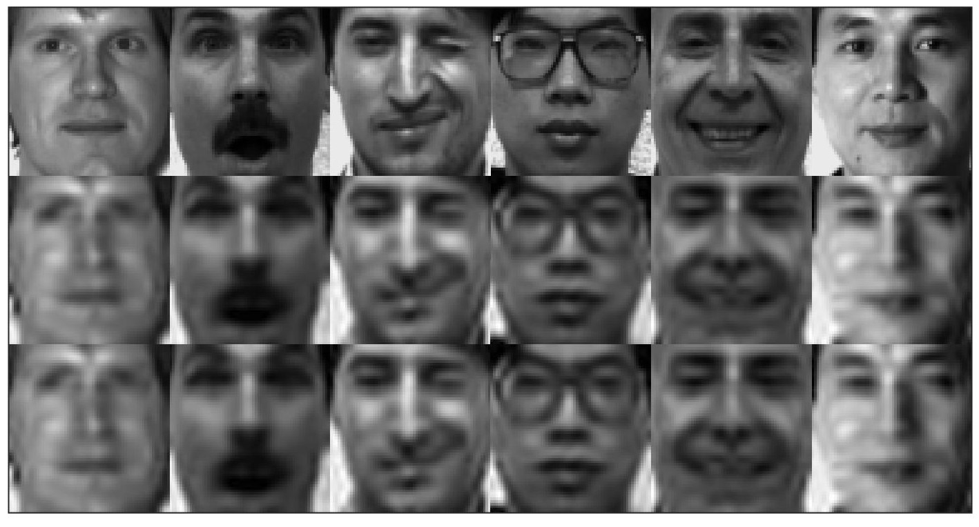
(a) 16x16

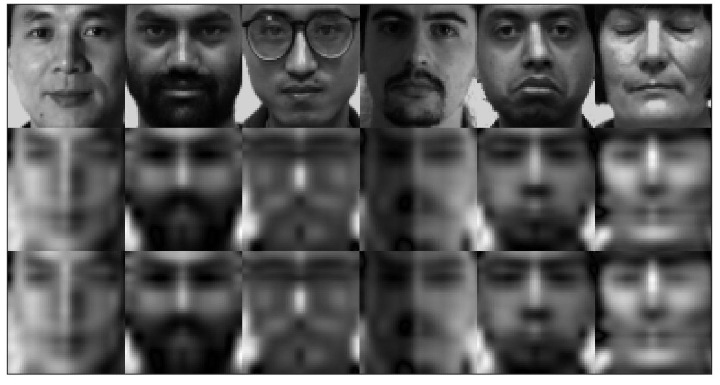
(b) 8x8

Figure 2: Compression of Yale face database (1th row) with HOOI (2th row) and RPCD+ (3th row)

The first row in each figure contains the original images, the second and third rows contain the results of the compression usin the HOOI and RPCD+ methods, respectively. The attained Relative error for both algorithms are the same but RPCD+ is faster ($0.12$ vs $0.19$ seconds) for the case of $16\times 16$. The difference in speed becomes larger ($0.09$ vs $0.16$ seconds), when we want to compress the data more, that is the case of $8\times 8$.

In another comparison for the real data, we compare RPCD, RPCD+ and HOOI with a newly introduced SVD-based method called D-Tucker [19]. D-Tucker compresses the original tensor by performing randomized SVD on slices of the re-ordered tensor and then computies the orthogonal factor matrices and the core tensor using SVD. [19] reported that this method works well when the order of a tensor is high in two dimensions and the rest of the orders are low, that is for $\mathcal{X}_{re}\in\mathbb{R}^{I_{1}\times I_{2}\times K_{3}\times...\times K_{d}}$ we have $I_{1}\geq I_{2}>>K_{3}\geq...\geq K_{d}$. Because, the term $L=K_{3}\times...\times K_{d}$, determines how many times the algorithm needs to do randomized SVDs for the slices.

Table 2: Execution time in seconds and relative error for the D-Tucker, RPCD, RPCD+ and HOOI methods on the real datasets.

Dataset	Yale [4]		Brainq [26]		Air Quality		HSI [13]		Coil-100 [28]
Dimension	[64 64 11 15]		[360 21764 9]		[30648 376 6]		[1021 1340 33 8]		[128 128 72 100]
Target Rank	[5 5 5 5]		[10 10 5]		[10 10 5]		[10 10 10 5]		[5 5 5 5]
	Time	Error	Time	Error	Time	Error	Time	Error	Time	Error
D-Tucker	0.17	30.47	1.02	77.26	0.91	33.85	4.80	45.13	5.61	36.65
RPCD	0.08	30.02	4.71	78.35	1.61	32.87	11.42	43.69	2.91	36.41
RPCD+	0.05	29.93	4.74	77.87	1.45	32.74	7.88	43.48	1.92	36.35
HOOI	0.07	29.92	86.46	77.92	68.21	32.72	8.06	43.42	1.48	36.35

(a) Brainq

(b) Air Quality

(c) HSI

(d) Coil-100

(e) Yale Face

Figure 3: Convergence behavior of different methods for the real datasets. Y-axis is the difference between the relative error at each iteration and the best achieved related error.

The comparative results on the real data are given in Table 2 and Fig. 3. Except D-Tucker that does not need any initialization, we initialize the factors matrices to have one at main diagonal and zero elsewhere as it is common for iterative eigen-solvers. As it can be seen in Table 2, The RPCD+ method almost always has better final relative error than RPCD, due to the precision update process. Sometimes it is also faster due to smaller number of iterations it needs to converge. In Air Quality and HSI datasets, the D-Tucker method has computational advantage, but as it can be seen in Fig. 3, this advantage is because it stops early and therefore it lacks good precision. For Yale and Coil-100 which have large $L$, D-Tucker lose its advantage meanwhile RPCD+ and HOOI do a good job in speed and precision. Both RPCD+ and HOOI present the best low multi-linear rank approximation, but HOOI is substantially slower when the dimensionality is high. An important observation from these experiment is that RPCD+, as a general method, has a solid performance in lower dimensions and superior performance in high-dimensional cases, which we saw also in the results of the synthetic data.

For all datasets except Brainq, we observe almost identical convergence behavior when we start at different starting points. The effect of different initialization on the performance of different methods for Brainq can be seen in Fig. 4.

(a)

(b)

(c)

(d)

(e)

(f)

Figure 4: Convergence behavior for decomposing the Brainq dataset using different random initializations.

6 Conclusion

In this paper, we introduced RPCD and its improved version RPCD+, first-order methods solving the Tucker Decomposition problem for high-order, high-dimensional dense tensors with Riemannian coordinate descent method. For these methods, we constructed a Riemannian metric by incorporating the second order information of the reformulated cost function and the constraint. We proved a convergence rate for general tangent subspace descent on Riemannian manifolds, which for the special case of product manifolds like Tucker Decomposition matches the rate in the Euclidean setting. Experimental results showed that RPCD+ as a general method has the best performance among competing methods for high-order, high-dimensional tensors.

For a future work, it would be interesting to examine the RPCD method in solving tensor completion problems. Another interesting line of thought would be to incorporating latent tensors between original tensor $\mathcal{X}$ and projected tensor $\mathcal{Y}$ for further reducing computation costs.

References

- [1] P.-A. Absil, R. Mahony, and R. Sepulchre, Optimization algorithms on matrix manifolds, Princeton University Press, Princeton, NJ, United States, 2009.
- [2] W. Austin, G. Ballard, and T. G. Kolda, Parallel tensor compression for large-scale scientific data, in IEEE International parallel and distributed processing symposium (IPDPS), 2016, pp. 912–922.
- [3] A. Beck and L. Tetruashvili, On the convergence of block coordinate descent type methods, SIAM journal on Optimization, 23 (2013), pp. 2037–2060.
- [4] P. N. Belhumeur, J. P. Hespanha, and D. J. Kriegman, Eigenfaces vs. Fisherfaces: Recognition using class specific linear projection, IEEE Transactions on Pattern Analysis and Machine Intelligence, 19 (1997), pp. 711–720.
- [5] N. Boumal, An introduction to optimization on smooth manifolds, Available online, May, (2020).
- [6] N. Boumal, P.-A. Absil, and C. Cartis, Global rates of convergence for nonconvex optimization on manifolds, IMA Journal of Numerical Analysis, 39 (2019), pp. 1–33.
- [7] N. Boumal, B. Mishra, P.-A. Absil, and R. Sepulchre, Manopt, a Matlab toolbox for optimization on manifolds, Journal of Machine Learning Research, 15 (2014), pp. 1455–1459, https://www.manopt.org.
- [8] M. Che and Y. Wei, Randomized algorithms for the approximations of Tucker and the tensor train decompositions, Advances in Computational Mathematics, 45 (2019), pp. 395–428.
- [9] A. Cichocki, R. Zdunek, A. H. Phan, and S.-i. Amari, Nonnegative matrix and tensor factorizations: applications to exploratory multi-way data analysis and blind source separation, John Wiley & Sons, West Sussex, United Kingdom, 2009.
- [10] L. De Lathauwer, B. De Moor, and J. Vandewalle, A multilinear singular value decomposition, SIAM Journal on Matrix Analysis and Applications, 21 (2000), pp. 1253–1278.
- [11] L. De Lathauwer, B. De Moor, and J. Vandewalle, On the best rank- and rank- approximation of higher-order tensors, SIAM journal on Matrix Analysis and Applications, 21 (2000), pp. 1324–1342.
- [12] L. Eldén and B. Savas, A Newton-Grassmann method for computing the best multilinear rank- approximation of a tensor, SIAM Journal on Matrix Analysis and applications, 31 (2009), pp. 248–271.
- [13] D. H. Foster, K. Amano, S. M. Nascimento, and M. J. Foster, Frequency of metamerism in natural scenes, Journal of the Optical Society of America A, 23 (2006), pp. 2359–2372.
- [14] G. H. Golub and C. F. Van Loan, Matrix computations, Johns Hopkins University Press, Baltimore, MD, United States, 1996.
- [15] L. Grasedyck, Hierarchical singular value decomposition of tensors, SIAM Journal on Matrix Analysis and Applications, 31 (2010), pp. 2029–2054.
- [16] D. H. Gutman and N. Ho-Nguyen, Coordinate descent without coordinates: Tangent subspace descent on Riemannian manifolds, arXiv preprint arXiv:1912.10627v2, (2019).
- [17] M. Haardt, F. Roemer, and G. Del Galdo, Higher-order svd-based subspace estimation to improve the parameter estimation accuracy in multidimensional harmonic retrieval problems, IEEE Transactions on Signal Processing, 56 (2008), pp. 3198–3213.
- [18] M. Ishteva, P.-A. Absil, S. Van Huffel, and L. De Lathauwer, Best low multilinear rank approximation of higher-order tensors, based on the Riemannian trust-region scheme, SIAM Journal on Matrix Analysis and Applications, 32 (2011), pp. 115–135.
- [19] J.-G. Jang and U. Kang, D-tucker: Fast and memory-efficient tucker decomposition for dense tensors, in IEEE International Conference on Data Engineering (ICDE), 2020, pp. 1850–1853.
- [20] H. Kasai and B. Mishra, Low-rank tensor completion: a Riemannian manifold preconditioning approach, in International Conference on Machine Learning (ICML), 2016, pp. 1012–1021.
- [21] T. G. Kolda and B. W. Bader, Tensor decompositions and applications, SIAM Review, 51 (2009), pp. 455–500.
- [22] T. G. Kolda and B. W. Bader, Tensor toolbox for MATLAB, version 3.2.1, 2021, https://www.tensortoolbox.org.
- [23] D. Kressner, M. Steinlechner, and B. Vandereycken, Low-rank tensor completion by riemannian optimization, BIT Numerical Mathematics, 54 (2014), pp. 447–468.
- [24] H. Lu, K. Plataniotis, and A. Venetsanopoulos, Mpca: Multilinear principal component analysis of tensor objects, IEEE Transactions on Neural Networks, 19 (2008), pp. 18–39.
- [25] B. Mishra and R. Sepulchre, Riemannian preconditioning, SIAM Journal on Optimization, 26 (2016), pp. 635–660.
- [26] T. M. Mitchell, S. V. Shinkareva, A. Carlson, K.-M. Chang, V. L. Malave, R. A. Mason, and M. A. Just, Predicting human brain activity associated with the meanings of nouns, Science, 320 (2008), pp. 1191–1195.
- [27] M. Mørup, L. K. Hansen, and S. M. Arnfred, Algorithms for sparse nonnegative Tucker decompositions, Neural Computation, 20 (2008), pp. 2112–2131.
- [28] S. A. Nene, S. K. Nayar, and H. Murase, Columbia object image library (COIL-100), Tech. Report CUCS-006-96, Department of Computer Science, Columbia University, 1996.
- [29] J. Oh, K. Shin, E. E. Papalexakis, C. Faloutsos, and H. Yu, S-hot: Scalable high-order Tucker decomposition, in ACM International Conference on Web Search and Data Mining (WSDM), 2017, pp. 761–770.
- [30] B. Savas and L.-H. Lim, Quasi-Newton methods on Grassmannians and multilinear approximations of tensors, SIAM Journal on Scientific Computing, 32 (2010), pp. 3352–3393.
- [31] N. D. Sidiropoulos, L. De Lathauwer, X. Fu, K. Huang, E. E. Papalexakis, and C. Faloutsos, Tensor decomposition for signal processing and machine learning, IEEE Transactions on Signal Processing, 65 (2017), pp. 3551–3582.
- [32] Y. Sun, Y. Guo, C. Luo, J. Tropp, and M. Udell, Low-rank Tucker approximation of a tensor from streaming data, SIAM Journal on Mathematics of Data Science, 2 (2020), pp. 1123–1150.
- [33] L. R. Tucker, Some mathematical notes on three-mode factor analysis, Psychometrika, 31 (1966), pp. 279–311.
- [34] N. Vannieuwenhoven, R. Vandebril, and K. Meerbergen, A new truncation strategy for the higher-order singular value decomposition, SIAM Journal on Scientific Computing, 34 (2012), pp. A1027–A1052.
- [35] S. J. Wright, Coordinate descent algorithms, Mathematical Programming, 151 (2015), pp. 3–34.
- [36] Y. Xu, On the convergence of higher-order orthogonal iteration, Linear and Multilinear Algebra, 66 (2018), pp. 2247–2265.
- [37] A. Zare, A. Ozdemir, M. A. Iwen, and S. Aviyente, Extension of PCA to higher order data structures: An introduction to tensors, tensor decompositions, and tensor PCA, Proceedings of the IEEE, 106 (2018), pp. 1341–1358.