Ordinal Pooling

Abstract

In the framework of convolutional neural networks, downsampling is often performed with an average-pooling, where all the activations are treated equally, or with a max-pooling operation that only retains an element with maximum activation while discarding the others. Both of these operations are restrictive and have previously been shown to be sub-optimal. To address this issue, a novel pooling scheme, named ordinal pooling, is introduced in this work. Ordinal pooling rearranges all the elements of a pooling region in a sequence and assigns a different weight to each element based upon its order in the sequence. These weights are used to compute the pooling operation as a weighted sum of the rearranged elements of the pooling region. They are learned via a standard gradient-based training, allowing to learn a behavior anywhere in the spectrum of average-pooling to max-pooling in a differentiable manner. Our experiments suggest that it is advantageous for the networks to perform different types of pooling operations within a pooling layer and that a hybrid behavior between average- and max-pooling is often beneficial. More importantly, they also demonstrate that ordinal pooling leads to consistent improvements in the accuracy over average- or max-pooling operations while speeding up the training and alleviating the issue of the choice of the pooling operations and activation functions to be used in the networks. In particular, ordinal pooling mainly helps on lightweight or quantized deep learning architectures, as typically considered e.g. for embedded applications. Code will be available at https://github.com/mistasse/ordinal-pooling-layers.

How to cite this work? This is the authors’ preprint version of a paper published at BMVC 2019. Please cite it as follows: A. Deliège, M. Istasse, A. Kumar, C. De Vleeschouwer and M. Van Droogenbroeck, "Ordinal Pooling", in British Machine Vision Conference, 2019.

1 Introduction

Convolutional neural networks (CNNs) [12] that are specifically suited for various visual tasks, such as image classification [11], object detection [17], segmentation [6], and modeling video evolution [3], are one of the main drivers of deep learning. A typical deep CNN architecture consists of three types of layers: 1) convolutional: for extracting various features or activations from an input image or feature maps, 2) pooling: a downsampling technique for aggregating elements within a pooling region so that the size of the feature maps along the spatial dimensions becomes smaller, and 3) fully connected: to carry out the classification from the extracted features at the end of the network. Many types of CNNs have been reported in the literature, for instance, network-in-network (NIN) [14], residual networks (ResNets) [7], inception networks [20], squeeze-and-excitation networks (SENets) [8], densely connected convolutional networks (DenseNets) [9].

Replicating convolution kernels across the spatial dimensions in CNNs enables weight sharing across space. This helps achieve equivariance, i.e. a translation of an object in an input image results in an equivalent translation in the activations of the output feature map. The pooling operation, on the other hand, tends to achieve translational invariance, i.e. a translation of an object in an input image does not influence the output of the network. This pooling operation is most commonly performed either by average-pooling (shortened to avg-pooling in the following), where all the activations in a pooling region are averaged together, or by max-pooling, where only the element with the maximum activation is retained. A theoretical analysis on these two pooling operations reveals that none of the techniques is optimal [2]. Yet, it has sometimes been argued that max-pooling achieves better performances over avg-pooling because avg-pooling treats all the elements equivalently irrespective of their activations, which results in an undervaluation of the elements with higher activations, while the elements with smaller activations are overestimated [18, 1].

This work presents an alternative pooling scheme, named ordinal pooling, that generalizes the classic avg- and max-pooling operations and resolves the issue of unfair valuation of the elements in a pooling region, while still preserving the information from other activations. In this scheme, all the elements in a pooling region are first ordered based upon their activations and then combined together via a weighted sum, where the weights are assigned depending upon the orders of the elements and are learned with a standard gradient-based optimization during the training phase. Moreover, a key difference between ordinal pooling and a classic pooling layer is that while a typical pooling acts upon each feature map in the same way, ordinal pooling learns a different set of weights for each feature map and therefore allows much more flexibility in the pooling layer.

2 Related Works

The idea of a rank-based weighted aggregation was first introduced by Kolesnikov et al. [10] in the context of image segmentation, who proposed a global weighted rank-pooling (GWRP) in order to estimate a score associated with a segmentation class. However, GWRP is used only as a global pooling procedure as it acts upon all the elements in a feature map to generate the score of a particular segmentation class. Also, contrary to ordinal pooling, the weights that are assigned based on the order of the elements are determined from a hyper-parameter and therefore do not change during the training.

In addition to GWRP [10], other variants of rank-based pooling have been introduced by Shi et al. [19], who proposed three pooling schemes based upon the rank of the elements: 1) average, 2) weighted, and 3) stochastic. Unlike ordinal pooling, all of these schemes require an additional hyperparameter, which is thus not learned in a differentiable way. Indeed, in the first scheme, the hyperparameter is fixed to determine the threshold for choosing the activations to be averaged. In the second scheme, it is fixed to generate the weights to be applied to the activations, which remain the same across all the feature maps, while in the third scheme, a set of probabilities is generated based upon this hyperparameter and is used to select an element in a pooling region.

Other works focus upon generalizing the pooling operation. Gulcehre et al. [5] regard pooling as a $l_{p}$ norm, where the values of $1$ and $\infty$ for the parameter $p$ correspond to avg- and max-pooling, whereas $p$ itself is learned during the training. Pinheiro et al. [16] use a smooth convex approximation of max-pooling, called Log-Sum-Exp, where a hyperparameter controls the smoothness of the approximation, so that pixels with similar scores have a similar weight in the training process. Lee et al. [13] propose mixing together avg-pooling and max-pooling by a trainable parameter and also introduce the idea of tree pooling to learn different pooling filters and combine these filters responsively.

Since a $2\times 2$ max-pooling with a stride of 2 in each spatial dimension discards $75\%$ of a feature map upon its application, it is an aggressive operation, which after a series of applications can result in a significant loss in information. To apply pooling in a gentler manner, a fractional max-pooling [4] has been proposed, where the dimensions of the feature map can be reduced by a non-integer factor. In the spirit of allowing information from other activations within a pooling region to also pass to the next layer, a stochastic version of pooling has been proposed by Zeiler et al. [21], where an element in a pooling region is selected based upon its probability within the multinomial distribution constructed from all the activations inside the pooling region. Another stochastic variant of pooling, S3Pool [22], is a two-step pooling technique, where in the first step, a $2\times 2$ pooling with a stride of $1$ is applied, while in the second step, a stochastic downsampling is performed. A combination of these operations makes S3Pool to work as a strong regularization technique.

3 Method

A pooling operator can be seen as a real-valued function $f_{P}$ defined on the finite non empty subsets of real numbers $\mathcal{P}_{\text{\text{fin}}}(\mathbb{R})=\{A\subset\mathbb{R}:0<|A|<+\infty\}$. In particular, the avg-pooling and max-pooling operators, noted $f_{P}^{\text{avg}}$ and $f_{P}^{\text{max}}$, are respectively defined by

$$f_{P}^{\text{avg}}(A)=\frac{1}{|A|}\sum_{a\in A}a,\ \ \ \ \ \ \ f_{P}^{\text{max}}(A)=\max\{a:a\in A\}.$$ (1)

In CNNs, a pooling layer is used to decrease the spatial resolution of the feature maps obtained after the application of a nonlinear activation on responses to trainable convolutional filters. A pooling layer thus transforms an input tensor $s\in\mathbb{R}^{H\times W\times C}$ of spatial resolution $H\times W$ with $C$ feature maps (or channels) to an output tensor $t\in\mathbb{\mathbb{R}}^{H^{\prime}\times W^{\prime}\times C}$ with $H^{\prime}<H$ and $W^{\prime}<W$. This is commonly done via a $m\times n$ pooling operation, which consists of slicing $s$ into $I$ pooling regions $R_{i}\in\mathbb{R}^{m\times n\times C}$ ($i\leq I$), and applying a same pooling operator $f_{P}$ to each channel $R_{i}^{c}\in\mathbb{R}^{m\times n}$ ($c\leq C$) in each $R_{i}$. In a conventional CNN, the same pooling operator $f_{P}\in\{f_{P}^{\text{avg}},f_{P}^{\text{max}}\}$ is used for all the feature maps and remains fixed as the network trains.

In this work, we introduce the ordinal pooling layer, whose pooling operator involves trainable weights that are specific to each feature map. In the case of a $m\times n$ ordinal pooling layer, a trainable weight kernel $w^{c}\in\mathbb{\mathbb{R}}^{m\times n}$ is used to pool the regions $R_{i}^{c}\in\mathbb{R}^{m\times n}$ ($i\leq I$) located on the feature map $c$ of the input tensor $s$. The ordinal pooling operator associated with $w^{c}$, defined on $\mathbb{R}^{m\times n}$, is given by

$$f_{P,w^{c}}^{\text{ord}}(R_{i}^{c})=w^{c}*\text{Ord}(R_{i}^{c})=\sum_{j\leq m,\,k\leq n}w_{j,k}^{c}\text{Ord}(R_{i}^{c})_{j,k}\enspace\mbox{,}$$ (2)

where $\text{Ord}()$ is a function from $\mathbb{R}^{m\times n}$ to $\mathbb{R}^{m\times n}$ that reorders the values of its input tensor based upon a given ranking process. In this work, we consider that $\text{Ord}(A)$ reorders the activations of a tensor $A\in\mathbb{R}^{m\times n}$ based upon the decreasing order of their values, such that for $j,j^{\prime}\leq m$ and $k,k^{\prime}\leq n$:

$$(j<j^{\prime})\lor(k<k^{\prime})\Rightarrow\text{Ord}(A)_{j,k}\geq\text{Ord}(A)_{j^{\prime},k^{\prime}}.$$ (3)

This implies that, for example, $w_{1,1}^{c}$(resp. $w_{m,n}^{c}$) always multiplies the largest (resp. smallest) value of $R_{i}^{c}$, for all $i\leq I$ and $c\leq C$. An illustration of $2\times 2$ ordinal pooling is represented in Figure 1. In practice, we constrain each kernel $w^{c}$ to contain only positive weights that sum to $1$. This is imposed to adhere to the common principle that a pooling operation is designed to aggregate the values comprised in a tensor and should thus output a value located in its convex hull. In particular, this guarantees that the output value is comprised between the minimum and the maximum values of the input tensor. An algorithm of the main workflow for the forward pass and the update of the weights is detailed in supplementary material to show how ordinal pooling can be implemented for the usual $2\times 2$ case. Let us note that, since ordinal pooling employs a different set of weights for each feature map, the total number of parameters introduced by this operation is $m\times n\times C$, which is negligible compared with convolutional and fully connected layers.

Ordinal pooling generalizes the commonly used avg- and max- pooling operators. Indeed, $m\times n$ avg-pooling is a particular case of ordinal pooling for which $w_{j,k}^{c}=1/(mn)$ for all $j\leq m$, $k\leq n$. Likewise, $m\times n$ max-pooling corresponds to the case where $w_{1,1}^{c}=1$ and $w_{j,k}^{c}=0$ for $(j,k)\neq(1,1)$. Also, compared with the other trainable pooling operations in the literature, ordinal pooling is the only technique that can lead to a min-pooling behavior.

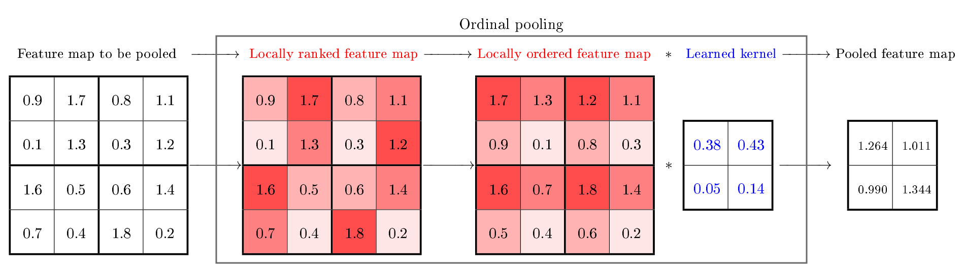
Figure 1: Example of $2\times 2$ ordinal pooling with stride 2 in each dimension for one feature map. The feature map to be pooled is sliced into $2\times 2$ regions, whose elements are ranked by decreasing order, i.e. in each region, the largest (resp. smallest) value has rank $1$ (resp. $4$) and is colored in dark (resp. light) red. Then, each region is reordered following the ranks of its elements and is convolved with the learned kernel associated with this feature map.

4 Experiments

4.1 Proof-of-concept

Setup.

We perform the following proof-of-concept experiment on MNIST. Let us consider a baseline network N comprising average pooling layers and its ordinal counterpart ON, wherein the average pooling layers are replaced by ordinal pooling layers. Since N and ON have the same structure, we initialize them exactly in the same way with the same weights for the non-pooling layers. The sole difference between N and ON is the additional weights required by ordinal pooling layers. These weights are initialized with “average pooling” initialization, i.e. for an ordinal pooling kernel of size $m\times n$, each weight is initialized as $1/(mn)$. This implies that, before starting the training of a baseline network N and its ON counterpart, the two networks are exactly in the same state, they produce the same output if they are fed with the same input. Moreover, we fix all the random seeds, so that the two networks will experience exactly the same batches of images, in the same order, the data augmentation is the same, at any time, over the course of their training. To guarantee the reproducibility of the experiments and avoid suffering from GPU-based non-determinism, these experiments are carried out on CPU. This setting allows us to compare the results of N and ON pairwise, for each run of the experiment, which provides a fairer and more significant insight on the intrinsic superiority of one network over the other.

Networks compared.

Three “baseline networks” are used in the experiment, described as follows with standard compact notations:

1. “Baseline”: $5\times 5$ Conv $\times 32$, $2\times 2$ pooling, $5\times 5$ Conv $\times 64$, $8\times 8$ global pooling, FC($10$), softmax.

2. “Baseline-2”: $3\times 3$ Conv $\times 16$ ZP, $2\times 2$ pooling, $3\times 3$ Conv $\times 32$ ZP, $2\times 2$ pooling, $3\times 3$ Conv $\times 64$ ZP, $7\times 7$ global pooling, FC($10$), softmax.

3. “LeNet5”: $5\times 5$ Conv $\times 6$ ZP, $2\times 2$ pooling, $5\times 5$ Conv $\times 16$, $2\times 2$ pooling, FC($120$), ReLU, FC($84$), ReLU, FC($10$), softmax.

These networks have their “ordinal” counterpart, e.g. “Ordinal baseline-2”, for which the layers “(global) pooling” are replaced by “(global) ordinal pooling”. As mentioned above, “(global) average pooling” are used as pooling layers in the classic pooling setting while “average pooling initialization” is used to instantiate the weights of the ordinal pooling kernels. More details about the training of these networks are provided in supplementary material.

Results.

Each network is run $100$ times, where the runs differ by their initial random seeds. Figure 2 shows the average learning curves for the network “Baseline” and its “Ordinal baseline” counterpart. It can be seen that ordinal pooling allows to reach better performances in terms of accuracy and loss, while it also speeds up the training process.

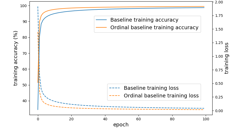
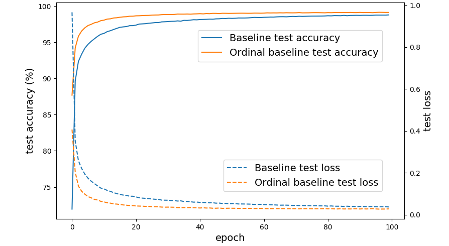
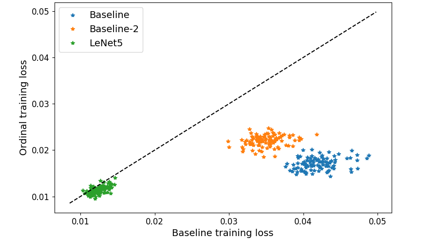
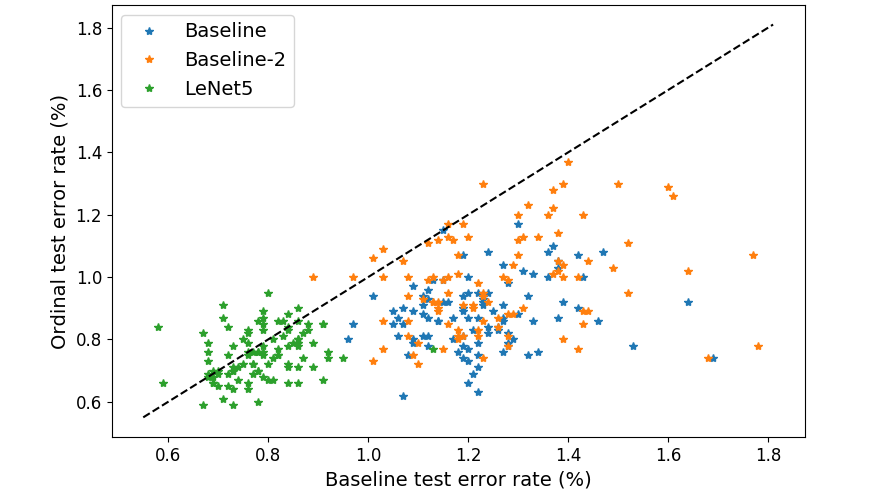
Figure 2: Average learning curves for the “Baseline” network and its “Ordinal baseline” counterpart and pairwise comparison of different runs (differing in random seeds initializations) of the networks with and without ordinal pooling having the same instantiation. Points under the black dotted line indicate better performances for networks with ordinal pooling.

The pairwise comparison of the performances of the networks versus their ordinal counterpart is represented in Figure 2. As can be seen, the “Baseline” and “Baseline-2” networks employing ordinal pooling always achieve smaller training loss at the end of the training. The same is also true for the “LeNet5” network $89\%$ of the time. Regarding test error rates, the ordinal pooling networks outperform the classic ones $100\%$, $94\%$, and $74\%$ of the time for the “Baseline”, “Baseline-2”, and “LeNet5” cases, respectively. Even though ordinal pooling seems less beneficial to LeNet5, the results have to be put in perspective with respect to the extra cost in parameters that the ordinal pooling layers require. In fact, as can be inferred from Table 1, LeNet5 has by far the best ratio between the relative improvement in performances (both in terms of average and variance in test error rate) and the number of additional parameters contained in the ordinal pooling layers. Table 1 suggests that overall, the performances of the networks are boosted with ordinal pooling by a comfortable margin through a reduced average test error rate, and that ordinal pooling provides a more consistent convergence between different runs, through a reduced variance in test error rate. These benefits come at a moderate cost in terms of number of parameters.

Relative variation in	Baseline	Baseline-2	LeNet5
average/variance of training loss	$-59\%/-70\%$	$-37\%/-66\%$	$-8\%/-25\%$
average/variance of test loss	$-25\%/-5\%$	$-21\%/-8\%$	$-5\%/-23\%$
average/variance of test error rate	$-28\%/-26\%$	$-22\%/-18\%$	$-4\%/-7\%$
number of parameters	$+8\%$	$+14\%$	$+0.14\%$

Table 1: Relative variation in some metrics when the avg-pooling layers of the baseline networks are replaced by ordinal pooling layers. Networks with ordinal pooling show a large decrease in the average and variance of the losses and error rates for a moderate increase in number of parameters.

Distribution of $2\times 2$ ordinal pooling kernels.

The use of ordinal pooling instead of a classic pooling operation allows to study the distributions of the weight kernels in the ordinal pooling layers, as learned by the networks, and helps discover how the trained networks chose to perform the pooling operations. For that purpose, we compare the learned kernels with some template kernels that characterize various categories of behaviors for the kernels, including avg- and max-pooling like behaviors. These template kernels are chosen based on the behavior that they induce as explained below.

In the case of a $2\times 2$ ordinal pooling layer, a weight kernel $w=\left[w_{1},w_{2},w_{3},w_{4}\right]$ leads to max-pooling if it converges to $[1,0,0,0]$ and to avg-pooling if each $w_{i}=1/4$. In the first case, the network “promotes” only the largest value of each pooling region, while in the second case, all the values are equally “promoted”. Nevertheless, a network may prefer to promote, for example, the lowest value of the regions (thus min-pooling behavior) by using the kernel $\left[0,0,0,1\right]$, or its first two largest values with $\left[1/2,1/2,0,0\right]$. The template kernels are determined based upon this idea of enumerating all the ways that some values can be promoted by the network. In fact, it has the possibility to promote any of the four ordered values of the regions by making $w$ converge to one of the following four template kernels:

$$\mathtt{w}_{\mathtt{1}}=\left[1,0,0,0\right],\ \mathtt{w}_{\mathtt{2}}=\left[0,1,0,0\right],\ \mathtt{w}_{\mathtt{3}}=\left[0,0,1,0\right],\ \mathtt{w}_{\mathtt{4}}=\left[0,0,0,1\right].$$

In the same spirit, it may prefer to promote equally two, three, or the four values of the ordered regions, making $w$ converge to

$$\mathtt{w}_{\mathtt{12}} =\left[\frac{1}{2},\frac{1}{2},0,0\right],\ \mathtt{w}_{\mathtt{13}}=\left[\frac{1}{2},0,\frac{1}{2},0\right],\ \mathtt{w}_{\mathtt{14}}=\left[\frac{1}{2},0,0,\frac{1}{2}\right],\ \mathtt{w}_{\mathtt{23}}=\left[0,\frac{1}{2},\frac{1}{2},0\right],\ \mathtt{w}_{\mathtt{24}}=\left[0,\frac{1}{2},0,\frac{1}{2}\right],\ \mathtt{w}_{\mathtt{34}}=\left[0,0,\frac{1}{2},\frac{1}{2}\right],$$

$$\mathtt{w}_{\mathtt{123}}=\left[\text{$\frac{1}{3}$},\text{$\frac{1}{3}$},\text{$\frac{1}{3}$},0\right],\ \mathtt{w}_{\mathtt{124}}=\left[\text{$\frac{1}{3}$},\text{$\frac{1}{3}$},0,\text{$\frac{1}{3}$}\right],\mathtt{w}_{\mathtt{134}}=\left[\text{$\frac{1}{3}$},0,\text{$\frac{1}{3}$},\text{$\frac{1}{3}$}\right],\ \mathtt{w}_{\mathtt{234}}=\left[0,\text{$\frac{1}{3}$},\text{$\frac{1}{3}$},\text{$\frac{1}{3}$}\right],\ \mathtt{w}_{\mathtt{1234}}=\left[\frac{1}{4},\frac{1}{4},\frac{1}{4},\frac{1}{4}\right].$$

We note $P_{i}$ the set of template kernels having $i$ non-zero values. After the training of a network, for each kernel of a $2\times 2$ ordinal pooling layer, we identify its closest template kernel, in term of Euclidean distance. We examine the distribution of the learned kernels by grouping them by “closest template kernels” to find out how the network chooses to perform the pooling operations. These distributions for ordinal pooling layers of “Baseline-2”, grouped by $P_{i}$ and aggregated for the $100$ runs, are displayed in Figure 3 (top left and top right).

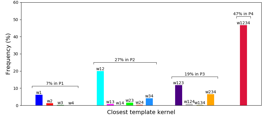
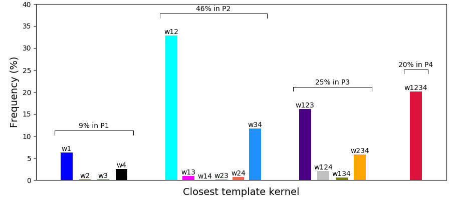
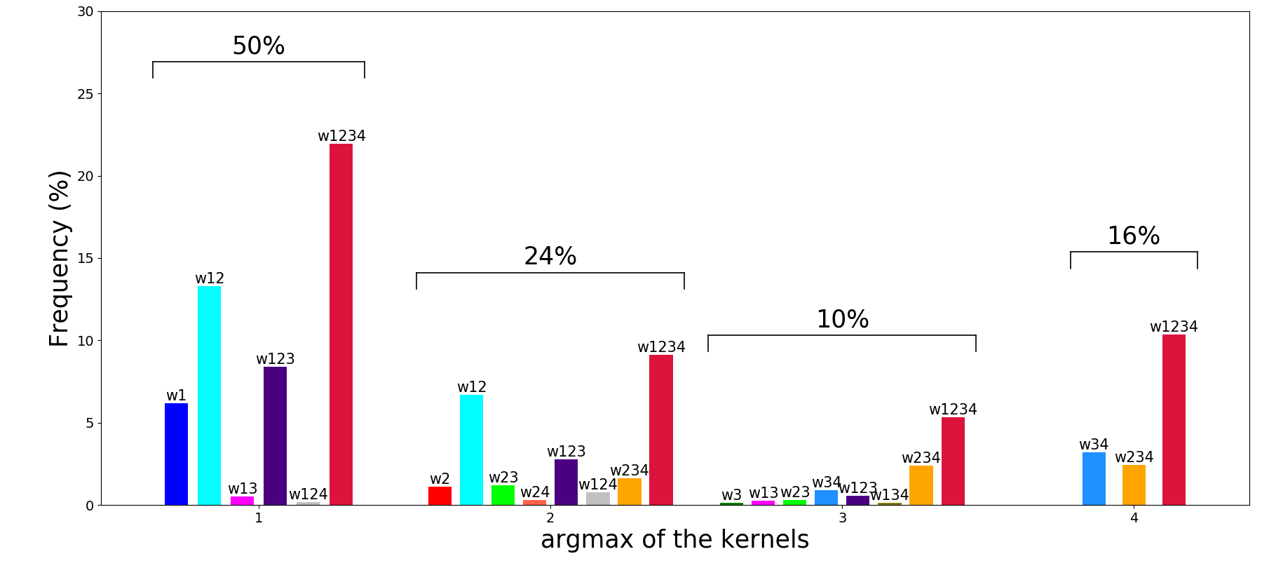
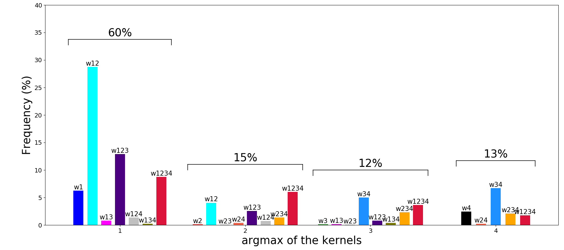
Figure 3: Distributions of the kernels of the first (left) and second (right) ordinal pooling layers of “Ordinal baseline-2” according to their closest template kernel, grouped by number of promoted values (top), and grouped by the index of their largest weight (bottom).

It can be seen that, even though all the kernels were initialized as $\mathtt{w}_{\mathtt{1234}},$ after the training less than half of them remain closer to $\mathtt{w}_{\mathtt{1234}}$ than to any other template kernel. Another observation is that the network seems to prefer promoting contiguous “extreme” (largest or smallest) values in the sorted regions, i.e. when $2$ (resp. $3$) values are promoted, the associated kernels are preferably closer to $\mathtt{w}_{\mathtt{12}}$ or $\mathtt{w}_{\mathtt{34}}$ (resp. $\mathtt{w}_{\mathtt{123}}$ or $\mathtt{w}_{\mathtt{234}}$). The “extreme” aspect is reinforced in the group $P_{1}$ of the top right plot, in which almost only $\mathtt{w}_{1}$ and $\mathtt{w}_{4}$ are present. Hence, some kernels actually display a “min-pooling” behavior.

Also, the network prefers to promote the largest value of the regions, which manifests by the fact that the argmax of a learned kernel is often $1$, thus indicating that a behavior between average pooling and max-pooling is often desired. This observation is illustrated in Figure 3 (bottom left and bottom right), where the kernels are first distributed according to their argmax, then sub-divided following their closest template kernel. Similar trends are also observed for “Ordinal baseline” and “Ordinal LeNet5” (provided in supplementary material). A complementary analysis of the kernels related to the global ordinal pooling layer is presented in supplementary material.

4.2 Influence of ordinal weights initialization

In this section, we examine the performances of the networks under various weight initializations in the ordinal pooling layers. As before, we report average test error rates over $100$ runs of each experiment to compare the results in Table 2.

For the $2\times 2$ ordinal pooling kernels, the initializations investigated are average, max, min. For the average (resp. max, min) case, each kernel is instantiated as $\mathtt{w}_{\mathtt{1234}}$ (resp. $\mathtt{w}_{\mathtt{1}}$,$\mathtt{w}_{\mathtt{4}}$). For the global $n\times n$ ordinal pooling layers, average pooling ($1/n^{2}$) is used.

Table 2 shows that the networks with ordinal pooling consistently outperform the classic ones. Also, the performances are less dependent on the initialization of the ordinal pooling kernels than they are in the classic setting. Ordinal pooling thus alleviates the problem of choosing the appropriate type of pooling layer to incorporate in the networks.

Max-pooling initialization performs better in this experiment. However, even with min-pooling initialization, the ordinal networks are still able to reach performances close to standard initializations, while it is not as clear for the classic networks. An explanation may reside in the use of ReLU activations before the pooling layers. In the classic setting, min-pooling forces the networks to select the lowest value of the pooled regions, hence it can be assumed that many zero values are propagated in the network, responsible for decreasing the amount of useful information and thus leading to lower performances. In the ordinal pooling setting, the network has enough flexibility to circumvent this fixed min-pooling behavior, and this only requires small variations in the ordinal weights. Indeed, we observed that the closest template kernel after the training was still most often $\mathtt{w}_{4}$.

We also examined a “uniform” initialization, where for each kernel, all the weights are randomly initialized with uniform distribution between $0$ and $1$ and are then normalized so as to sum to $1$. The results do not differ much from those obtained with “average” initialization and are discussed in supplementary material.

Pooling	$2\times 2$	glob.	Bas.	Bas.-2	LN5		Activation Bas.-2
							None	ReLU	tanh
classic	average	average	1.22	1.26	0.79		49.50	1.26	1.62
ordinal	average	average	0.89	1.00	0.75		1.13	1.00	0.99
classic	max	average	0.98	1.01	0.74		3.69	1.01	1.58
ordinal	max	average	0.82	0.89	0.71		1.01	0.89	0.90
classic	min	average	1.48	1.34	0.94		3.82	1.34	1.55
ordinal	min	average	0.97	1.02	0.84		1.05	1.02	0.90

Table 2: (Left) Average test error rates (in $\%$) for various weight initializations in the pooling layers. For classic pooling, the weights are not trainable. (Right) Corresponding average test error rates for “Baseline-2” and its ordinal counterpart with various activation functions.

4.3 Influence of activation functions

The case of the ordinal min-pooling initialization raises the question of the influence of the activation function used before the pooling operation. We thus compare the average test error rates of various initializations and three types of activation functions: “None” (no activation), “ReLU”, “tanh”. The results for the “Baseline-2” structure are reported in Table 2.

The results obtained for a given initialization with ordinal pooling are less sensitive to the choice of the activation function than those obtained in the networks with classic pooling schemes. Conversely, for a given activation, the results with ordinal pooling are less sensitive to the choice of initialization compared to the networks employing classic poolings.

One of the most striking results may be related to the performances obtained without any activation. Indeed, while it is well-known that CNNs need non-linear activations to achieve competitive performances, the networks with ordinal pooling layers still manage to obtain good performances without activation. In this case, some are even better than others obtained in the classic setting with activations. The sorting procedure in the ordinal pooling layer is itself a non-linearity, which explains these results. This is especially true for the avg-pooling case, where it is known that an avg-pooling layer without prior activation is useless. For better performances, it still appears that using an activation is beneficial even with ordinal pooling layers, but the choice of the function may not be as crucial as in the networks with classic pooling. Similar trends were observed with “Baseline” and “LeNet5” structures.

4.4 Results on other datasets and best use cases

Ordinal pooling can be used in any CNN architecture involving pooling layers. Its benefits vary from one use case to another, as indicated by the following additional results, reported as average test error rates on five trials. On CIFAR10, with a CNN made of five Conv(128)-ReLU-Pooling blocks and a FC layer, ordinal pooling outperforms avg-pooling ($13.16\%$ vs $14.21\%$). With DenseNet-BC-100-12 [9], the results are mostly equivalent with ordinal and avg-pooling ($5.53\%$ vs $5.45\%$ with ReLU, $6.35\%$ vs $6.85\%$ with tanh) except without activation ($12.51\%$ vs $59.39\%$), similarly to CIFAR100 ($24.73\%$ vs $24.74\%$ with ReLU, $27.01\%$ vs $27.05\%$ with tanh, $37.39\%$ vs $81.61\%$ without activation).

Even though exhaustive performance-related experiments still need to be carried out as future work, the present results are in line with those reported previously and confirm that ordinal pooling mainly helps on relatively simple architectures, as typically considered e.g. for embedded applications. To further support this statement, we performed experiments with quantized networks, as described in [15]. It appears that the more the model is quantized, the more ordinal pooling helps: with quantized versions of ResNet-14 (resp. ResNet-20), on CIFAR10, ordinal pooling performs up to $3.5$ (resp. $1.1\%$) better than max-pooling. It also reduces the gap between binary ResNet-14 and -20, which is of $0.7\%$, against $2.7\%$ with max-pooling, which certainly opens interesting prospects for ordinal pooling, as it helps simpler models achieve performances comparable with more complex models.

For the record, our experiments on MNIST and CIFAR10 with [13] lead to results comparable with those presented above with ordinal pooling ($<1\%$ difference). A comprehensive comparison with the pooling methods present in the literature could be the subject of a survey article (along with defining benchmark tests to assess the performances of a pooling method), and is thus beyond the scope of this work.

5 Conclusion

A novel trainable pooling scheme, Ordinal Pooling, is introduced in this work, which operates in two steps. In the first step, all the elements of a pooling region are reordered in decreasing sequence. Then, a trainable weight kernel is convolved with the rearranged pooling region to compute the output of the ordinal pooling operation. The usual avg- and max-pooling operations can be recovered as particular cases of ordinal pooling.

In our experiments, replacing classic avg- and max-pooling operations with ordinal pooling produces large relative improvements in classification performances at a moderate cost in additional parameters and also leads to a faster convergence. Ordinal pooling allows to perform the pooling operation differently in distinct feature maps. The analysis of the learned kernels reveals that the networks take advantage of this extra flexibility by using various types of pooling for different feature maps within the same pooling layer. A general trend is that a hybrid behavior between avg- and max-pooling is often desired, even though the lowest elements of the pooling regions are not always discarded. Moreover, the performances of the networks are less inclined to fluctuate when different initializations of the ordinal pooling kernels are used than when different classic pooling operations are imposed. Besides, even when no non-linear activation function is applied after the convolutional layers, the intrinsic non-linearity introduced by ordinal pooling alone generally suffices to produce performances which are better than either avg- and max-pooling used along with activation functions. Finally, our experiments suggest that ordinal pooling might be of particular interest for lightweight or quantized architectures, as typically considered in e.g. embedded resource-constrained systems.

As future work, as already mentioned, it will be interesting to perform more experiments with more datasets and various architectures to determine the configurations which best benefit from the ordinal pooling operation. From a technical point of view, the value of the elements of the pooling regions is chosen as the criterion for ordering the region. However, other criteria could also be envisioned to further extend the ordinal pooling scheme. Eventually, conducting experiments with our baseline models but with other types of pooling methods proposed in the literature is certainly our next step in order to rank ordinal pooling among available pooling operations.

Acknowledgements

This research is supported by the DeepSport project of the Walloon region, Belgium, C. De Vleeschouwer is funded by the F.R.S.-FNRS.

References

- [1] Y. Boureau, N. Le Roux, F. Bach, J. Ponce, and Y. Lecun. Ask the locals: Multi-way local pooling for image recognition. In IEEE Int. Conf. Comput. Vision (ICCV), pages 2651–2658, Barcelona, Spain, Nov. 2011.
- [2] Y. Boureau, J. Ponce, and Y. LeCun. A theoretical analysis of feature pooling in visual recognition. In Int. Conf. Mach. Learn. (ICML), pages 111–118, Haifa, Israel, June 2010.
- [3] B. Fernando, E. Gavves, M. Jose Oramas, A. Ghodrati, and T. Tuytelaars. Modeling video evolution for action recognition. In IEEE Int. Conf. Comput. Vision and Pattern Recogn. (CVPR), pages 5378–5387, Boston, MA, USA, June 2015.
- [4] B. Graham. Fractional max-pooling. CoRR, abs/1412.6071, Dec. 2014.
- [5] C. Gulcehre, K. Cho, R. Pascanu, and Y. Bengio. Learned-norm pooling for deep feedforward and recurrent neural networks. In Machine Learning and Knowledge Discovery in Databases, volume 8724 of Lecture Notes Comp. Sci., pages 530–546. Springer, 2014.
- [6] K. He, G. Gkioxari, P. Dollar, and R. Girshick. Mask R-CNN. In IEEE Int. Conf. Comput. Vision (ICCV), pages 2980–2988, Venice, Italy, Oct. 2017.
- [7] K. He, X. Zhang, S. Ren, and J. Sun. Deep residual learning for image recognition. In IEEE Int. Conf. Comput. Vision and Pattern Recogn. (CVPR), pages 770–778, Las Vegas, NV, USA, June 2016.
- [8] J. Hu, L. Shen, and G. Sun. Squeeze-and-excitation networks. CoRR, abs/1709.01507, 2017.
- [9] G. Huang, Z. Liu, L. van der Maaten, and K. Weinberger. Densely connected convolutional networks. In IEEE Int. Conf. Comput. Vision and Pattern Recogn. (CVPR), pages 2261–2269, Honolulu, HI, USA, July 2017.
- [10] A. Kolesnikov and C. Lampert. Seed, expand and constrain: Three principles for weakly-supervised image segmentation. In Eur. Conf. Comput. Vision (ECCV), volume 9908 of Lecture Notes Comp. Sci., pages 695–711. Springer, 2016.
- [11] A. Krizhevsky, I. Sutskever, and G. Hinton. ImageNet classification with deep convolutional neural networks. In Adv. in Neural Inform. Process. Syst. (NeurIPS), volume 25, pages 1097–1105, 2012.
- [12] Y. Lecun, L. Bottou, Y. Bengio, and P. Haffner. Gradient-based learning applied to document recognition. Proc. of IEEE, 86(11):2278–2324, Nov. 1998.
- [13] C.-Y. Lee, P. Gallagher, and Z. Tu. Generalizing pooling functions in CNNs: Mixed, gated, and tree. IEEE Trans. Pattern Anal. Mach. Intell., 40(4):863–875, Apr. 2018.
- [14] M. Lin, Q. Chen, and S. Yan. Network in network. CoRR, abs/1312.4400, Dec. 2013.
- [15] B. Moons, K. Goetschalckx, N. Van Berckelaer, and M. Verhelst. Minimum energy quantized neural networks. In Asilomar Conference on Signals, Systems, and Computers, pages 1921–1925, Pacific Grove, CA, USA, 2017.
- [16] P. O. Pinheiro and R. Collobert. From image-level to pixel-level labeling with convolutional networks. In IEEE Int. Conf. Comput. Vision and Pattern Recogn. (CVPR), jun 2015.
- [17] S. Ren, K. He, R. Girshick, and J. Sun. Faster R-CNN: Towards real-time object detection with region proposal networks. IEEE Trans. Pattern Anal. Mach. Intell., 39(6):1137–1149, June 2017.
- [18] D. Scherer, A. Müller, and S. Behnke. Evaluation of pooling operations in convolutional architectures for object recognition. In Int. Conf. Artificial Neural Networks (ICANN), volume 6354 of Lecture Notes Comp. Sci., pages 92–101. Springer, 2010.
- [19] Z. Shi, Y. Ye, and Y. Wu. Rank-based pooling for deep convolutional neural networks. Neural Networks, 83:21–31, Nov. 2016.
- [20] C. Szegedy, S. Ioffe, V. Vanhoucke, and A. Alemi. Inception-v4, Inception-ResNet and the impact of residual connections on learning. In AAAI Conf. Artificial Intell., pages 4278–4284, San Francisco, CA, USA, Feb. 2017.
- [21] M. Zeiler and R. Fergus. Stochastic pooling for regularization of deep convolutional neural networks. In Int. Conf. on Learn. Rep. (ICLR), Scottsdale, Arizona, May 2013.
- [22] S. Zhai, H. Wu, A. Kumar, Y. Cheng, Y. Lu, Z. Zhang, and R. Feris. S3Pool: Pooling with stochastic spatial sampling. In IEEE Int. Conf. Comput. Vision and Pattern Recogn. (CVPR), pages 4003–4011, Honolulu, HI, USA, July 2017.