Variational Bayes Algorithm and Posterior Consistency of Ising Model Parameter Estimation

Abstract

Ising models originated in statistical physics and are widely used in modeling spatial data and computer vision problems. However, statistical inference of this model remains challenging due to intractable nature of the normalizing constant in the likelihood. Here, we use a pseudo-likelihood instead to study the Bayesian estimation of two-parameter, inverse temperature, and magnetization, Ising model with a fully specified coupling matrix. We develop a computationally efficient variational Bayes procedure for model estimation. Under the Gaussian mean-field variational family, we derive posterior contraction rates of the variational posterior obtained under the pseudo-likelihood. We also discuss the loss incurred due to variational posterior over true posterior for the pseudo-likelihood approach. Extensive simulation studies validate the efficacy of mean-field Gaussian and bivariate Gaussian families as the possible choices of the variational family for inference of Ising model parameters.

, and

1 Introduction

A popular way of modeling a spatially dependent binary vector $\boldsymbol{x}=(x_{1},\dots,x_{n})^{\top}$ is to take advantage of Ising model named after the physicist Ernst Ising [17] which has been used in a wide range of applications including spatial data analysis and computer vision. Many different versions of Ising model have emerged in the literature. In this paper, we focus on two-parameter Ising model, which has an inverse temperature parameter $\beta>0$ and a magnetization parameter $B\neq 0$, with a symmetric coupling matrix $A_{n}\in\mathbb{R}^{n\times n}$. An Ising model is often represented by an undirected graph in which each vertex represents $x_{i}\in\{-1,1\}$ and the connections between $x_{i}$’s are determined by $A_{n}$. Here, $\beta$ characterizes the strength of interactions among $x_{i}$’s and $B$ represents external influence on $\boldsymbol{x}$. In the first place, Ising model has been introduced for the relations between atom spins [6] with the domain $\{-1,1\}^{n}$. While we work with the domain $\{-1,1\}^{n}$, in many current applications, Ising model has been defined with different domain $\{0,1\}^{n}$. One can read [15] for more details on two different domains.

Estimation of Ising model parameters has received considerable attention in statistics and computer science literature. The existing literature can be broadly divided into two groups. Some literature assume that i.i.d. (independently and identically distributed) copies of data ($\boldsymbol{x}$ vector) are available for inference, [1], [5], [22], [26], and [29]. Another category of literature assumes that only one sample is observable, [3], [8], [9], [10], [11], [12], and [13]. Under the assumption of only one observation, [10] showed that the MLE of $\beta>0$ for Curie-Weiss model is consistent if $B\neq 0$ is known, and vice versa. They also proved that the joint MLE does not exist when neither $\beta$ nor $B$ is given. In this regard, [11] addressed joint estimation of $(\beta,B)$ using pseudo-likelihood and showed that the pseudo-likelihood estimator is consistent under some conditions on coupling matrix $A_{n}$.

Some previous studies which utilized Bayesian methodology along with Ising model include those of [20] which explored Bayesian variable selection with Ising prior to capture structural information. [21] proposed a joint Ising and Dirichlet Process (Ising-DP) prior for simultaneous selection and clustering in Bayesian framework. In their PhD thesis, [30] dealt with estimation of parameters of Ising and Potts models using Bayesian approach. All these works assume replicated data and do not provide theoretical validation. In this article, we provide a Bayesian estimation methodology for model parameters in an Ising model when one observes the data only once.

Methodological Contribution: One of the main challenges in the Bayesian estimation of Ising models lies in the intractable nature of the normalizing constant in the likelihood. Following the works of [11], [3] and [24], we replace the true likelihood of the Ising model by a pseudo-likelihood. As a first contribution, we establish that the posterior based on the pseudo-likelihood is consistent for a suitable choice of the prior distribution. Further, we use variational Bayes (VB) approach which has recently become a popular and computationally powerful alternative to MCMC. In order to approximate the unknown posterior distribution using VB, we need to choose an appropriate variational family. We propose a Gaussian mean field family and general bivariate normal family with transformation of the parameters to $(\log\beta,B)$. For implementation of VB, we employ a black box variational inference (BBVI), [25]. In BBVI, we need to evaluate the likelihood to compute the gradient estimate. But the existence of an unknown normalizing constant in likelihood of Ising model prevents us using BBVI directly. So, we use pseudo-likelihood as in [11]. Replacing the true likelihood of Ising model with pseudo-likelihood, we are able to compute all the quantities needed for implementing BBVI.

Theoretical Contribution: The main theoretical contribution of this work lies in establishing the consistency of the variational posterior for the Ising model with the true likelihood replaced by the pseudo-likelihood. In this direction, we first establish the rates at which the true posterior based on the pseudo-likelihood concentrates around the $\varepsilon_{n}$- shrinking neighborhoods of the true parameter. With a suitable bound on the Kulback-Leibler distance between the true and the variational posterior, we next establish the rate of contraction for the variational posterior and demonstrate that the variational posterior also concentrates around $\varepsilon_{n}$-shrinking neighborhoods of the true parameter. These results have been derived under three set of assumptions on the coupling matrix $A_{n}$ (see section 3 for more details). Indeed, we demonstrate that the variational posterior consistency holds for the same set of assumptions on $A_{n}$ as those needed for the convergence of the maximum likelihood estimates based on the pseudo-likelihood. One of the main caveats in establishing the posterior contraction rates under the pseudo-likelihood structure is in ensuring that the concentration of the variational posterior occurs in $\mathbb{P}_{0}^{(n)}$ probability where $\mathbb{P}_{0}^{(n)}$ is the distribution induced by the true likelihood and not the pseudo-likelihood. Indeed, we could show that in $\mathbb{P}_{0}^{(n)}$ probability, the contraction of variational posterior happens at the rate $1-1/M_{n}$ in contrast to the faster rate $1-\exp(-Cn\varepsilon_{n}^{2}),C>0$ for the true posterior. As a final theoretical contribution, we establish that the variational Bayes estimator convergences to the true parameters at the rate $1/\varepsilon_{n}$ where $\varepsilon_{n}$ can be chosen $n^{-\delta}$, $0<\delta<1/2$ provided the $A_{n}$ matrix satisfies certain regularity assumptions.

The rest of the paper is organized as follows: Section 2 defines the likelihood and pseudo-likelihood of Ising model with two parameters $(\beta,B)$ and provides the details of our Bayesian estimation using variational inference approach. In Section 3 we discuss our main theoretical developments and sketch of the proof. The details of the proof are deferred to the Appendix. The numerical studies are provided in Section 4. We give a comparison of our variational Bayes estimates to existing maximum likelihood estimators based on pseudo-likelihood.

2 Model and methods

2.1 Ising model

For a representation of an Ising model with two parameters $\beta>0$ and $B\neq 0$, consider an undirected graph which has $n$ vertices $x_{i}$, $i=1,\dots,n$. Each vertex of the graph takes a value either -1 or 1, i.e., $x_{i}\in\{-1,1\}$. Then, we define a likelihood of Ising model as the probability of the vector $\boldsymbol{x}=(x_{1},\dots,x_{n})^{\top}\in\{-1,1\}^{n}$:

$$\mathbb{P}_{\beta,B}^{(n)}(\boldsymbol{X}=\boldsymbol{x})=\frac{1}{Z_{n}(\beta,B)}\exp\left(\frac{\beta}{2}\boldsymbol{x}^{\top}A_{n}\boldsymbol{x}+B\sum_{i=1}^{n}x_{i}\right),$$ (1)

where $Z_{n}(\beta,B)$ is a normalizing constant which makes sum of (1) over the support $\{-1,1\}^{n}$ equal to 1. $A_{n}$ is a coupling matrix of size $n\times n$ which determines the connections between the coordinates of $\boldsymbol{x}$. More precisely, let $\mathcal{E}=\{(i,j)\mid i\sim j,~{}1\leq i,j\leq n\}$ be the set of edges in the graph where $i\sim j$ denote that the vertices $i$ and $j$ are connected. Then $A_{n}$ is a symmetric matrix with $A_{n}(i,j)=0$ for all $(i,j)\notin\mathcal{E}$ and $A_{n}(i,j)>0$ for all $(i,j)\in\mathcal{E}$.

For the purpose of this paper, we work with a scaled adjacency matrix $A_{n}$ whose all diagonal elements are zeros and the other elements are non-negative.

Definition 2.1 (Scaled adjacency matrix).

A scaled adjacency matrix for a graph $G_{n}$ with $n$ vertices is defined as:

$$A_{n}(i,j):=\begin{cases}\frac{n}{2|G_{n}|}&\mbox{if }(i,j)\in\mathcal{E}\\ 0&\mbox{otherwise.}\end{cases},$$

where $|G_{n}|$ denotes the number of edges.

In our study, we assume that only one $\boldsymbol{x}\in\{-1,1\}^{n}$ is observed. In this regard, estimating all the elements of $A_{n}$ is impossible because $A_{n}$ has $n(n-1)/2$ distinct values. In this work, we primarily focus on the problem of estimation of the parameters $(\beta,B)$ under the assumption of a fully known coupling matrix $A_{n}$. The same set up considered by [3], [11], and [24].

2.2 Pseudo-likelihood

It is challenging to use the likelihood (1) directly because of the unknown normalizing constant $Z_{n}(\beta,B)$. Due to the intractable nature of the likelihood, the standard Bayesian implementation is computationally intractable. We thereby propose the use of the conditional probability of $x_{i}$ given others. It is easily calculated because $x_{i}$ is binary:

$$\mathbb{P}_{\beta,B}^{(n)}\big{(}X_{i}=1|X_{j},j\neq i\big{)}=\frac{e^{\beta m_{i}(\boldsymbol{x})+B}}{e^{\beta m_{i}(\boldsymbol{x})+B}+e^{-\beta m_{i}(\boldsymbol{x})-B}},$$

where $m_{i}(\boldsymbol{x})=\sum_{j=1}^{n}A_{n}(i,j)x_{j}$.

The pseudo-likelihood of Ising model corresponding to the likelihood in (1), is defined as the product of one dimensional conditional distributions (see [11], for further details):

$$\prod_{i=1}^{n}\mathbb{P}_{\beta,B}^{(n)}\left(X_{i}=x_{i}\mid X_{j},j\neq i\right)$$

$$=2^{-n}\exp\left(\sum_{i=1}^{n}\left(\beta x_{i}m_{i}(\boldsymbol{x})+Bx_{i}-\log\cosh(\beta m_{i}(\boldsymbol{x})+B)\right)\right).$$ (2)

Our subsequent Bayesian development will make use of the pseudo-likelihood (2.2) instead of the true likelihood (1). We shall establish that the posterior obtained by the use of the pseudo-likelihood allows for consistent estimation of the model parameters $\beta$ and $B$.

2.3 Bayesian formulation

Let $\theta=(\beta,B)$ be the parameter set of interest. We consider the following independent prior distribution $p(\theta)=p_{\beta}(\beta)p_{B}(B)$, with $p_{\beta}(\beta)$ as a log-normal prior for $\beta$ and $p_{B}(B)$ as a normal prior for $B$ as follows:

$$p_{\beta}(\beta) =\frac{1}{\beta\sqrt{2\pi}}e^{-\frac{(\log\beta)^{2}}{2}},\hskip 14.22636ptp_{B}(B)=\frac{1}{\sqrt{2\pi}}e^{-\frac{B^{2}}{2}}.$$ (3)

The assumption of log-normal prior on $\beta$ is to ensure the positivity of $\beta$. Let $L(\theta)$ be the pseudo-likelihood function given by (2.2), then the above prior structure leads to the following posterior distribution

$$\Pi(\mathcal{A}\mid X^{(n)})=\frac{\int_{\mathcal{A}}\pi(\theta,X^{(n)})d\theta}{m(X^{(n)})}=\frac{\int_{\mathcal{A}}L(\theta)p(\theta)d\theta}{\int L(\theta)p(\theta)d\theta},$$ (4)

for any set $\mathcal{A}\subseteq\Theta$ where $\Theta$ denotes the parameter space of $\theta$. Note, $\pi(\theta,X^{(n)})$ is the joint density of $\theta$ and the data $X^{(n)}$ and $m(X^{(n)})$ is the marginal density of $X^{(n)}$ which is free from the parameter set $\theta$.

2.4 Variational inference

Next, we need to provide a variational approximation to the posterior distribution (4). In this direction, we consider two choices of the variational family to obtain approximated posterior distribution. One candidate of our variational family, for the virtue of simplicity, is a mean-field (MF) Gaussian family:

$$\mathcal{Q}^{\bf MF}=\bigg{\{}q(\theta)\mid~{}q(\theta)=q_{\beta}(\beta)q_{B}(B),\log\beta\sim N(\mu_{1},\sigma_{1}^{2}),B\sim N(\mu_{2},\sigma_{2}^{2})\bigg{\}},$$ (5)

The above variational family is the same as a lognormal distribution on $\beta$ and normal distribution on $B$. Also, $\beta$ and $B$ are independent in $\mathcal{Q}^{\bf MF}$ and each $q(\theta)\in\mathcal{Q}^{\bf MF}$ is governed by its own parameter set $\nu^{\bf MF}=(\mu_{1},\mu_{2},\sigma_{1}^{2},\sigma_{2}^{2})^{\top}$. $\nu^{\bf MF}$ denote the set of variational parameters which will be updated to find the optimal variational distribution closest to the true posterior.

Beyond the mean field family, we suggest a bivariate normal (BN) family to exploit the interdependence among the parameters $(\beta,B)$:

$$\mathcal{Q}^{\bf BN}=\Bigg{\{}q(\theta)\mid~{}q(\theta)=q(\beta,B),(\log\beta,B)\sim MVN(\boldsymbol{\mu},\boldsymbol{\Sigma}),\boldsymbol{\mu}=\begin{pmatrix}\mu_{1}\\ \mu_{2}\end{pmatrix},\boldsymbol{\Sigma}=\begin{pmatrix}\sigma_{11}&\sigma_{12}\\ \sigma_{12}&\sigma_{22}\end{pmatrix}\Bigg{\}}$$ (6)

$\mathcal{Q}^{\bf MF}$ can also be represented as (independent) bivariate normal family. The variational parameters of BN family are $\nu^{\bf BN}=(\mu_{1},\mu_{2},\sigma_{11},\sigma_{22},\sigma_{12})^{\top}$.

Once a variational family is chosen, one can find the variational posterior by minimizing the Kullback-Leibler (KL) divergence between a variational distribution $q\in\mathcal{Q}$ and the true posterior (4). The variational posterior is thus given by

$$Q^{*}=\underset{Q\in\mathcal{Q}}{\arg\min}~{}{\rm KL}(Q,\Pi(\mid X^{(n)})),$$ (7)

where ${\rm KL}(Q,\Pi(\mid X^{(n)}))$ is the KL divergence given by

$${\rm KL}(Q,\Pi(\mid X^{(n)}))=\int\log(q(\theta)/\pi(\theta\mid X^{(n)}))q(\theta)d\theta,$$

where $q$ and $\pi(\mid X^{(n)})$ are the densities corresponding to $Q$ and $\Pi(\mid X^{(n)})$ respectively. Based on $\eqref{true_po}$, we re-write the KL divergence as:

$${\rm KL}(Q,\Pi(\mid X^{(n)})) =\int(\log q(\theta)-\log\pi(\theta,X^{(n)}))q(\theta)d\theta+\log m(X^{(n)})$$

$$=-{\rm ELBO}(Q,\Pi(,X^{(n)}))+\log m(X^{(n)}).$$

The first term is the negative Evidence Lower Bound (ELBO) and observe that the second term does not depend on $q$. Therefore, minimizing KL divergence is equivalent to maximizing the ELBO. So, we search for an optimal $q$ by maximizing the ELBO:

$$Q^{*}=\underset{Q\in\mathcal{Q}}{\arg\max}~{}{\rm ELBO}(Q,\Pi(,X^{(n)})).$$

To optimize the ELBO, we consider the ELBO as a function of variational parameters $\nu$:

$$\mathcal{L}(\nu):=\mathbb{E}_{Q}(\log\pi(\theta,X^{(n)})-\log q(\theta;\nu)).$$

[25] suggested black box variational inference (BBVI) to optimize $\mathcal{L}(\nu)$ using gradient descent method. The gradient of $\mathcal{L}(\nu)$ is:

$$\nabla_{\nu}\mathcal{L} =\nabla_{\nu}\mathbb{E}_{Q}(\log\pi(\theta,X^{(n)})-\log q(\theta;\nu))$$

$$=\int q(\theta;\nu)\nabla_{\nu}\log q(\theta;\nu)(\log\pi(\theta,X^{(n)})-\log q(\theta;\nu))d\theta$$

$$\enskip+\int q(\theta;\nu)\nabla_{\nu}(\log\pi(\theta,X^{(n)})-\log q(\theta;\nu))d\theta$$

$$=\mathbb{E}_{Q}(\nabla_{\nu}\log q(\theta;\nu)(\log\pi(\theta,X^{(n)})-\log q(\theta;\nu))).$$ (8)

The last equality holds because $\mathbb{E}_{Q}(\nabla_{\nu}\log q(\theta;\nu))=0$ and $\nabla_{\nu}\log\pi(\theta,X^{(n)})=0$. We cannot exactly compute the expectation form (2.4) of the gradient $\nabla_{\nu}\mathcal{L}$, which lead us to employ Monte Carlo estimates:

$$\widehat{\nabla}_{\nu}\mathcal{L}=\frac{1}{S}\sum_{s=1}^{S}\nabla_{\nu}\log q(\theta^{(s)};\nu)(\log\pi(\theta^{(s)},X^{(n)})-\log q(\theta^{(s)};\nu)),$$ (9)

where $\theta^{(1)},\dots,\theta^{(S)}$ are samples generated from $q(\theta;\nu)$. Using the estimate $\eqref{mc_grad}$, we iteratively update $\nu$ in the direction of increasing the objective function $\mathcal{L}(\nu)$. The summary of BBVI algorithm is shown in Algorithm 1:

Result: Optimal variational parameters $\nu^{*}$

1 Initialize $p(\theta)$, $q(\theta;\nu^{1})$ and learning rate sequence $\rho_{t}$.

2 while ELBO increases do

3       Draw $\theta^{(s)}\sim q(\theta;\nu^{t})$, $s=1,\dots,S$;

4       Get $\widehat{\nabla}_{\nu}\mathcal{L}$ based on the $S$ sample points ;

5       Update $\nu^{t+1}\leftarrow\nu^{t}+\rho_{t}\widehat{\nabla}_{\nu}\mathcal{L}$ ;

6      

7 end while

Algorithm 1 BBVI

In Algorithm 1, $\rho_{t}$, $t=1,2,\cdots$ denotes a sequence of learning rates which satisfy the Robbin-Monro conditions [27], i.e. $\sum_{t=1}^{\infty}\rho_{t}=\infty$ and $\quad\sum_{t=1}^{\infty}\rho_{t}^{2}<\infty$. Also, let $\sigma\in\nu$ be a variational parameter which must be positive. During the updating procedure, it may occur that $\sigma$ takes a negative value. In order to preclude this issue, we consider a reparametrization $\sigma=\log(1+e^{\eta})$ and update the quantity $\eta$, as a free parameter, instead of updating $\sigma$. We address more details of BBVI algorithm implementation in Supplement Section A.1.

3 Main Theoretical Results

In this section, we establish the posterior consistency of the variational posterior (7). In this direction, we establish the variational posterior contraction rates to evaluate how well the posterior distribution of $\beta$ and $B$ under the variational approximation concentrates around the true values $\beta_{0}$ and $B_{0}$. Towards the proof, we make the following assumptions

Assumption 1 (Bounded row sums of $A_{n}$).

The row sums of $A_{n}$ are bounded above

$$\max_{i\in[n]}\sum_{j=1}^{n}A_{n}(i,j)\leq\gamma,$$

for a constant $\gamma$ independent of $n$. Assumption 1 is the same as (1.2) in [11]. As a consequence of assumption 1, it can be shown $m_{i}(\boldsymbol{x})\leq\gamma$, $i=1\dots,n$.

Assumption 2 (Mean field assumption on $A_{n}$).

Let $\epsilon_{n}\rightarrow 0$ and $n\epsilon_{n}^{2}\rightarrow\infty$ such that

$$(i)\>\>\sum_{i=1}^{n}\sum_{j=1}^{n}A_{n}(i,j)=O(n\epsilon_{n}^{2}),\hskip 28.45274pt(ii)\>\>\sum_{i=1}^{n}\sum_{j=1}^{n}A_{n}(i,j)^{2}=o(n\epsilon_{n}^{2}).$$

Assumption 2-$(i)$ is the same as condition (1.4) in [11] on $A_{n}$ for $\epsilon_{n}=1$. Assumption 2-$(ii)$ is the same as (1.6) in [11] with $\epsilon_{n}=1$. For more details on the mean field assumption, we refer to Definition 1.3 in [2].

Assumption 3 (Bounded variance of $A_{n}$).

Let $\bar{A}_{n}=(1/n)\sum_{i=1}^{n}\sum_{j=1}^{n}A_{n}(i,j)$,

$$\liminf_{n\to\infty}\frac{1}{n}\sum_{i=1}^{n}(\sum_{j=1}^{n}A_{n}(i,j)-\bar{A}_{n})^{2}>0.$$

Finally, the Assumption 3 corresponds to (1.7) in [11]. The validity of Assumption 3 ensures that $T_{n}(\boldsymbol{x})=(1/n)\sum_{i=1}^{n}(m_{i}(\boldsymbol{x})-\bar{m}(\boldsymbol{x}))^{2}$ is bounded below and above in probability, an essential requirement towards the proof of contraction rates of the variational posterior.

Let $\theta=(\beta,B)$ be the model parameter and $\theta_{0}=(\beta_{0},B_{0})$ be the true parameter from which the data $X^{(n)}$ is generated. Let $L(\theta)$ and $L(\theta_{0})$ denote the pseudo-likelihood as in (2.2) under the model parameter and true parameter respectively. Further, let $L_{0}$ denote the true probability mass function from which $X^{(n)}$ is generated. Thus, $L_{0}$ is as in (1) with $\theta=\theta_{0}$. We shall use the notations $\mathbb{E}_{0}^{(n)}$ and $\mathbb{P}_{0}^{(n)}$ to denote expectation and probability mass function with respect to $L_{0}$.

We next present the main theorem which establishes the contraction rate for the variational posterior. Following the proof, we next establish the contraction rate of the variational Bayes estimator as a corollary. We shall use the term with dominating probability to imply that under $\mathbb{P}_{0}^{(n)}$, the probability of the event goes to 1 as $n\to\infty$.

Theorem 3.1 (Posterior Contraction).

Let $\mathcal{U}_{\varepsilon_{n}}=\{\theta:||\theta-\theta_{0}||_{2}\leq\varepsilon_{n}\}$ be neighborhood of the true parameters. Suppose $\epsilon_{n}$ satisfies assumption 2., then in $\mathbb{P}_{0}^{(n)}$ probability

$$Q^{*}(\mathcal{U}_{\varepsilon_{n}}^{c})\to 0,\>\>n\to\infty,$$

where $\varepsilon_{n}=\epsilon_{n}\sqrt{M_{n}\log n}$ for any slowly increasing sequence $M_{n}\to\infty$ satisfying $\varepsilon_{n}\to 0$.

The above result establishes that the posterior distribution of $\beta$ and $B$ concentrates around the true value $\beta_{0}$ and $B_{0}$ at a rate slight larger than $\epsilon_{n}$. The proof of the above theorem rests on following lemmas, whose proofs have been deferred to the appendix A.

Lemma 3.2.

There exists a constant $C_{0}>0$, such that for any $\epsilon_{n}\rightarrow 0$, $n\epsilon_{n}^{2}\rightarrow\infty$,

$$\mathbb{P}_{0}^{(n)}\left(\log\int_{\mathcal{U}_{\epsilon_{n}}^{c}}\frac{L(\theta)}{L(\theta_{0})}p(\theta)d\theta\leq-C_{0}n\epsilon_{n}^{2}\right)\rightarrow 1,\>\>n\to\infty.$$

Lemma 3.3.

Let $\epsilon_{n}$ be the sequence satisfying the Assumption 2, then for any $C>0$,

$$\mathbb{P}_{0}^{(n)}\left(\Big{|}\log\int\frac{L(\theta)}{L(\theta_{0})}p(\theta)d\theta\Big{|}\leq Cn\epsilon_{n}^{2}\log n\right)\rightarrow 1.$$

Lemma 3.4.

Let $\epsilon_{n}$ be the sequence satisfying Assumption 2, then for some $Q\in\mathcal{Q}^{\bf MF}$ and any $C>0$,

$$\mathbb{P}_{0}^{(n)}\left(\int\log\frac{L(\theta_{0})}{L(\theta)}q(\theta)d\theta\leq Cn\epsilon_{n}^{2}\log n\right)\rightarrow 1.$$

Lemma 3.2 and Lemma 3.3 taken together suffice to establish the posterior consistency of the true posterior based on the likelihood $L(\theta)$ as in (4). Lemma 3.4 on the other hand is the additional condition which needs to hold to ensure the consistency of the variational posterior. We next state an important result which relates the variational posterior to the true posterior.

Formula for KL divergence: By Corollary 4.15 in [4],

$${\rm KL}(P_{1},P_{2})=\sup_{f}\left[\int fdP_{1}-\log\int e^{f}dP_{2}\right].$$

Using the above formula in the context of variational distributions, we get

$$\int fdQ^{*}\leq{\rm KL}(Q^{*},\Pi(\mid X^{(n)}))+\log\int e^{f}d\Pi(\mid X^{(n)}).$$ (10)

The above relation serves as an important tool towards the proof of Theorem 3.1. Next, we provide a brief sketch of the proof. Further details on the proof have been deferred to appendix B.

Sketch of proof of Theorem 3.1:

Let $f=(C_{0}/2)n\varepsilon_{n}^{2}1[\theta\in\mathcal{U}_{\varepsilon_{n}}^{c}]$, then

$$(C_{0}/2)n\varepsilon_{n}^{2}Q^{*}(\mathcal{U}_{\varepsilon_{n}}^{c})\leq{\rm KL}(Q^{*},\Pi(\mid X^{(n)}))+\log(e^{(C_{0}/2)n\varepsilon_{n}^{2}}\Pi(\mathcal{U}_{\varepsilon_{n}}^{c}\mid X^{(n)})+\Pi(\mathcal{U}_{\varepsilon_{n}}\mid X^{(n)}))$$

$$\implies Q^{*}(\mathcal{U}_{{\varepsilon_{n}}}^{c})\leq\frac{2}{C_{0}n\varepsilon_{n}^{2}}{\rm KL}(Q^{*},\Pi(\mid X^{(n)}))+\frac{2}{C_{0}n\varepsilon_{n}^{2}}\log(1+e^{(C_{0}/2)n\varepsilon_{n}^{2}}\Pi(\mathcal{U}_{{\varepsilon_{n}}}^{c}\mid X^{(n)})).$$

By Lemma 3.3 and 3.4, it can be established with dominating probability for any $C>0$, as $n\to\infty$

$${\rm KL}(Q^{*},\Pi(\mid X^{(n)}))\leq Cn\epsilon_{n}^{2}\log n.$$

By Lemma 3.2 and 3.3, it can be established with dominating probability, as $n\to\infty$

$$\Pi(\mathcal{U}_{{\varepsilon_{n}}}^{c}\mid X^{(n)})\leq e^{-C_{1}n\varepsilon_{n}^{2}},$$ (11)

for any $C_{1}>C_{0}/2$. Therefore, with dominating probability

$$Q^{*}(\mathcal{U}_{{\varepsilon_{n}}}^{c})\leq\frac{2C}{C_{0}M_{n}}+\frac{2}{C_{0}n\varepsilon_{n}^{2}}\log(1+e^{-(C_{1}-C_{0}/2)n\varepsilon_{n}^{2}})\sim\frac{2C}{C_{0}M_{n}}+\frac{e^{-(C_{1}-C_{0}/2)n\varepsilon_{n}^{2}}}{C_{0}n\varepsilon_{n}^{2}}\to 0.$$ (12)

This completes the proof.

Note that (11) gives the statement for the contraction of the true posterior. Similarly the contraction rate for the variational posterior follows as a consequence of (12). An important difference to note is that $Q^{*}(\mathcal{U}_{\varepsilon_{n}}^{c})$ goes to 0 at the rate $1/M_{n}$ in contrast to the faster rate $e^{-C_{1}n\varepsilon_{n}^{2}}$ for the true posterior.

Note, Theorem 3.1 gives the contraction rate of the variational posterior. However, the convergence of the of variational Bayes estimator to the true values of $\beta_{0}$ and $B_{0}$ is not immediate. The following corollary gives the convergence rate for the variational Bayes estimate as long as assumptions 1, 2 and 3 hold.

Corollary 3.5 (Variational Bayes Estimator Convergence).

Let $\varepsilon_{n}$ be as in Theorem 3.1, then in $\mathbb{P}_{0}^{(n)}$ probability,

$$\frac{1}{\varepsilon_{n}}\mathbb{E}_{Q^{*}}(||\theta-\theta_{0}||_{2})\to 0,\>\>n\to\infty.$$

Next, we provide a brief sketch of the proof. Further details of the proof have been deferred to appendix B.

Sketch of proof of Corollary 3.5: Let $f=(C_{2}/2)n\varepsilon_{n}||\theta-\theta_{0}||_{2}$, then

$$(C_{2}/2) n\varepsilon_{n}\int||\theta-\theta_{0}||_{2}dQ^{*}(\theta)$$

$$\leq{\rm KL}(Q^{*},\Pi(|X^{(n)}))+\log(\int e^{C_{2}n\varepsilon_{n}||\theta-\theta_{0}||_{2}/2}d\Pi(\theta|X^{(n)})).$$

By Lemma 3.3 and 3.4, it can be established with dominating probability, for any $C>0$

$${\rm KL}(Q^{*},\Pi(|X^{(n)}))\leq Cn\epsilon_{n}^{2}\log n.$$

By Lemma 3.2, and 3.3, it can be established with dominating probability, for some $C_{2}>0$

$$\int e^{(C_{2}/2)n\varepsilon_{n}||\theta-\theta_{0}||_{2}}d\Pi(\theta|X^{(n)})\leq\frac{1}{(C_{2}/2)n\varepsilon_{n}^{2}}e^{Cn\epsilon_{n}^{2}\log n}.$$ (13)

Therefore, with dominating probability

$$\int||\theta-\theta_{0}||_{2}dQ^{*}(\theta)\leq\frac{2C\varepsilon_{n}}{C_{2}M_{n}}-\frac{2\log(C_{2}/2)}{C_{2}n\varepsilon_{n}}-\frac{2\varepsilon_{n}\log(n\varepsilon_{n}^{2})}{C_{2}n\varepsilon_{n}^{2}}+\frac{2C\varepsilon_{n}}{C_{2}M_{n}}\leq\varepsilon_{n}o(1).$$

This completes the proof.

(13) follows as a consequence of convergence of the true posterior. An important thing to note that if $\varepsilon_{n}$ can be made arbitrarily close to $n^{-\delta}$ for $0<\delta<1/2$, it guarantees close to $\sqrt{n}$ convergence.

4 Simulation Results

4.1 Generating observed data

For numerical implementation, we need a coupling matrix $A_{n}$ and an observed vector $\boldsymbol{x}$ from (1). First, for generating a random $d$-regular graph and its scaled adjacency matrix, we used a python package NetworkX. Using the scaled adjacency matrix as our coupling matrix $A_{n}$, we facilitate $Metropolis$–$Hastings$ algorithm to generate an observed vector $\boldsymbol{x}$ with true parameters $(\beta_{0},B_{0})$ as follows:

• Define $H(\boldsymbol{x})=\frac{\beta_{0}}{2}\boldsymbol{x}^{\top}A_{n}\boldsymbol{x}+B_{0}\sum_{i=1}^{n}x_{i}$ and start with a random binary vector $\boldsymbol{x}=(x_{1},\dots,x_{n})^{\top}$.

• Randomly choose a spin $x_{i}$, $i\in\{1,\dots,n\}$.

• Flip the chosen spin, i.e. $x_{i}=-x_{i}$, and calculate $\Delta H=H(\boldsymbol{x}_{new})-H(\boldsymbol{x}_{old})$ due to this flip.

• The probability that we accept $\boldsymbol{x}_{new}$ is:

  $$\mathbb{P}(\text{accept}~{}\boldsymbol{x}_{new})=\begin{cases}1,&\text{if}\,\Delta H>0,\\ \exp\left(\Delta H\right),&\text{otherwise}.\end{cases}$$

• If rejected, put the spin back, i.e. $x_{i}=-x_{i}$.

• Go to 1 until the maximum number of iterations ($L$) is reached.

• After $L=1,000,000$ iterations, the last result is a sample $\boldsymbol{x}$ we use.

One can read [18] for more details of sampling from Ising model.

4.2 Performance Comparison

We compare the performance of the parameter estimation methods for two-parameter Ising model (1) under various combinations of $(d,n)$ and $(\beta_{0},B_{0})$. $Mean~{}squared~{}error(MSE)$ is used as the measurement for assessing the performances. With the given coupling matrix $A_{n}$ for each scenario, we repeat following steps $R$ times:

• Generate an observed vector $\boldsymbol{x}$ from (1) with true parameters $(\beta_{0},B_{0})$.

• Using the proposed BBVI algorithm with MF family or BN family, obtain the optimal variational distribution $q^{*}$ .

• Get $\hat{\theta}=(\hat{\beta},\hat{B})^{\top}$ as the sample means based on the samples drawn from $q^{*}$.

We use $S=200$ or $S=2000$ as the Monte Carlo sample size. Figure 1. in the Supplement Section A.2 describes ELBO convergence for the two different sample sizes with MF family and BN family. The figure indicates that the ELBO converges well with a moderate choice of $S$. Further, for faster convergence, one might choose BN family over mean-field family for variational distributions.

After we get $R=100$ pairs of estimates $(\hat{\beta}_{1},\hat{B}_{1}),\dots,(\hat{\beta}_{R},\hat{B}_{R})$, $MSE$ is calculated as:

$$MSE=\frac{1}{R}\sum_{r=1}^{R}\left(\left(\hat{\beta}_{r}-\beta_{0}\right)^{2}+\big{(}\hat{B}_{r}-B_{0}\big{)}^{2}\right).$$ (14)

First, we choose moderate values of $\beta_{0}=0.2,0.7$ with $B_{0}=\pm 0.2$, $\pm 0.5,\pm 0.8$. For each pair of $(\beta_{0},B_{0})$ we take $d=10,50$. The simulation results show that the $MSE$ values of our BBVI algorithm are smaller than PMLE from [11] for most cases. The two numbers in each cell of Table 1, 2, and 3 represent $MSE$ values when $n=100$ and $n=500$ respectively.

Table 1: Mean squared errors and computation times for each pair of $(\beta_{0},B_{0})$ when $n=100$ (left numbers) and $n=500$ (right numbers) given the degree of underlying graph $(d)$.

Degree of	Method	Monte Carlo	$(0.2,0.2)$	$(0.2,-0.2)$	$(0.7,0.2)$	$(0.7,-0.2)$	Convergence
graph ($d$)		samples ($S$)					time (sec)
10	PMLE	-	0.116 / 0.051	0.090 / 0.022	0.512 / 0.074	0.555 / 0.083	1.5 / 3.3
	MF family	200	0.121 / 0.060	0.105 / 0.030	0.180 / 0.073	0.326 / 0.083	30.4 / 60.0
		2000	0.107 / 0.052	0.092 / 0.021	0.137 / 0.076	0.267 / 0.076	120.3 / 245.9
	BN family	200	0.100 / 0.047	0.084 / 0.019	0.204 / 0.075	0.324 / 0.084	32.8 / 68.0
		2000	0.095 / 0.045	0.077 / 0.016	0.202 / 0.071	0.305 / 0.073	122.9 / 251.2
50	PMLE	-	0.555 / 0.101	0.414 / 0.163	1.158 / 0.333	0.938 / 0.386	1.5 / 3.6
	MF family	200	0.187 / 0.079	0.168 / 0.161	0.065 / 0.183	0.075 / 0.182	30.7 / 60.2
		2000	0.155 / 0.072	0.144 / 0.107	0.070 / 0.144	0.080 / 0.155	120.1 / 246.6
	BN family	200	0.293 / 0.065	0.236 / 0.148	0.102 / 0.174	0.085 / 0.178	31.5 / 68.1
		2000	0.213 / 0.090	0.178 / 0.143	0.081 / 0.176	0.063 / 0.185	123.1 / 250.8

PMLE, pseudo maximum likelihood estimate [11]; MF, mean-field; BN, bivariate normal.

Table 2: Mean squared errors and computation times for each pair of $(\beta_{0},B_{0})$ when $n=100$ (left numbers) and $n=500$ (right numbers) given the degree of underlying graph $(d)$.

Degree of	Method	Monte Carlo	$(0.2,0.5)$	$(0.2,-0.5)$	$(0.7,0.5)$	$(0.7,-0.5)$	Convergence
graph ($d$)		samples ($S$)					time (sec)
10	PMLE	-	0.272 / 0.053	0.126 / 0.067	1.048 / 0.232	1.240 / 0.261	1.5 / 3.2
	MF family	200	0.194 / 0.055	0.116 / 0.072	0.130 / 0.150	0.141 / 0.146	30.1 / 60.1
		2000	0.144 / 0.041	0.098 / 0.051	0.126 / 0.151	0.122 / 0.132	120.5 / 244.3
	BN family	200	0.231 / 0.042	0.136 / 0.046	0.172 / 0.144	0.239 / 0.136	31.9 / 67.5
		2000	0.217 / 0.047	0.130 / 0.058	0.156 / 0.140	0.220 / 0.133	122.1 / 250.3
50	PMLE	-	1.282 / 0.196	0.777 / 0.239	1.900 / 0.765	1.923 / 1.216	1.4 / 3.1
	MF family	200	0.144 / 0.113	0.128 / 0.234	0.089 / 0.162	0.086 / 0.254	30.3 / 60.0
		2000	0.120 / 0.048	0.108 / 0.097	0.099 / 0.197	0.100 / 0.157	120.4 / 245.1
	BN family	200	0.320 / 0.105	0.296 / 0.138	0.053 / 0.138	0.070 / 0.194	32.0 / 67.9
		2000	0.296 / 0.126	0.274 / 0.183	0.053 / 0.107	0.065 / 0.135	123.4 / 251.7

PMLE, pseudo maximum likelihood estimate [11]; MF, mean-field; BN, bivariate normal.

Table 3: Mean squared errors and computation times for each pair of $(\beta_{0},B_{0})$ when $n=100$ (left numbers) and $n=500$ (right numbers) given the degree of underlying graph $(d)$.

Degree of	Method	Monte Carlo	$(0.2,0.8)$	$(0.2,-0.8)$	$(0.7,0.8)$	$(0.7,-0.8)$	Convergence
graph ($d$)		samples ($S$)					time (sec)
10	PMLE	-	0.240 / 0.136	0.123 / 0.124	1.502 / 0.667	1.125 / 0.828	1.5 / 3.0
	MF family	200	0.151 / 0.110	0.126 / 0.104	0.128 / 0.142	0.105 / 0.215	30.2 / 60.2
		2000	0.127 / 0.080	0.111 / 0.067	0.083 / 0.121	0.079 / 0.171	120.0 / 242.9
	BN family	200	0.274 / 0.120	0.210 / 0.106	0.337 / 0.211	0.244 / 0.303	32.0 / 67.1
		2000	0.264 / 0.123	0.213 / 0.111	0.294 / 0.134	0.225 / 0.219	121.8 / 251.0
50	PMLE	-	0.922 / 0.494	1.756 / 0.517	2.592 / 2.773	2.510 / 1.933	1.5 / 3.1
	MF family	200	0.157 / 0.142	0.170 / 0.120	0.275 / 0.125	0.283 / 0.119	30.3 / 60.0
		2000	0.138 / 0.049	0.140 / 0.044	0.288 / 0.138	0.292 / 0.156	120.5 / 242.5
	BN family	200	0.431 / 0.160	0.496 / 0.223	0.318 / 0.130	0.358 / 0.086	32.1 / 67.0
		2000	0.417 / 0.183	0.474 / 0.196	0.305 / 0.094	0.347 / 0.074	121.5 / 251.2

PMLE, pseudo maximum likelihood estimate [11]; MF, mean-field; BN, bivariate normal.

For moderate values of $\beta_{0}$ (Table 1, 2, and 3), there is no significant difference between MF family and BN family in terms of $MSE$. When the interaction parameter $\beta_{0}$ is large, BN family seems to perform better. Table 4 shows all results for $\beta_{0}=1.2$.

Table 4: Mean squared errors and computation times for each pair of $(\beta_{0},B_{0})$ when $n=100$ (left numbers) and $n=500$ (right numbers) given the degree of underlying graph $(d)$.

Degree of	Method	Monte Carlo	$(1.2,0.2)$	$(1.2,-0.2)$	$(1.2,0.5)$	$(1.2,-0.5)$	Convergence
graph ($d$)		samples ($S$)					time (sec)
10	PMLE	-	1.681 / 0.379	1.677 / 0.496	2.687 / 1.483	2.716 / 1.598	1.6 / 3.0
	MF family	200	0.544 / 0.315	0.578 / 0.428	0.501 / 0.627	0.498 / 0.737	30.1 / 60.2
		2000	0.573 / 0.417	0.625 / 0.534	0.532 / 0.700	0.514 / 0.814	120.8 / 241.8
	BN family	200	0.404 / 0.309	0.409 / 0.374	0.247 / 0.488	0.248 / 0.479	32.2 / 66.9
		2000	0.396 / 0.295	0.405 / 0.368	0.235 / 0.411	0.234 / 0.449	121.3 / 250.7
50	PMLE	-	2.941 / 2.302	3.252 / 1.509	2.830 / 3.190	5.631 / 3.526	1.5 / 3.1
	MF family	200	0.775 / 0.998	0.771 / 0.775	0.832 / 0.836	0.810 / 0.792	30.0 / 60.3
		2000	0.812 / 1.022	0.818 / 1.025	0.868 / 0.972	0.862 / 0.947	120.5 / 241.4
	BN family	200	0.308 / 0.580	0.286 / 0.518	0.376 / 0.336	0.369 / 0.294	31.9 / 67.0
		2000	0.321 / 0.644	0.285 / 0.496	0.380 / 0.272	0.376 / 0.208	121.0 / 250.1

PMLE, pseudo maximum likelihood estimate [11]; MF, mean-field; BN, bivariate normal.

The numerical studies validate the superiority of our proposed variational Bayes based method. For more practical applications, we used our algorithm to regenerate an image matrix in the next subsection.

4.3 Data Reconstruction

The Ising model can be used for constructing an image in computer vision problem. In particular, the Bayesian procedure facilitate the reconstruction easily by using the posterior predictive distribution [14]. Consider an image in which each pixel represents either $-1(white)$ or $1(black)$. For choice of coupling matrix $A_{n}$, we use four-nearest neighbor structure and construct corresponding scaled adjacency matrix [16]. Then, we can generate such images following the steps in the subsection 4.1 with a true parameter pair $(\beta_{0},B_{0})$ and use it as our given data $\boldsymbol{x}$. With the generated image $\boldsymbol{x}$ and coupling matrix $A_{n}$, we obtain $(\hat{\beta},\hat{B})$ after implementing the parameter estimation procedure based on BN family. The estimates $(\hat{\beta},\hat{B})$ are used for data regeneration following the steps in the subsection 4.1 again. In Figure 1, we plot two original images in left column. The first original image was generated with $\beta_{0}=1.2,B_{0}=0.2$ and we use $\beta_{0}=1.2,B_{0}=-0.2$ for the second one. Also, in the right column, there are two corresponding images regenerated. It seems that, using our two-parameter Ising model and VI method with BN family, we can reconstruct the overall tendency of black and white images fairly well. For more precise pixel-by-pixel reconstruction, one can utilize multiple external parameters, $\boldsymbol{B}=(B_{1},\dots,B_{n})^{\top}$.

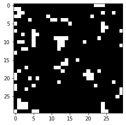
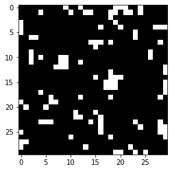
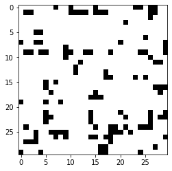
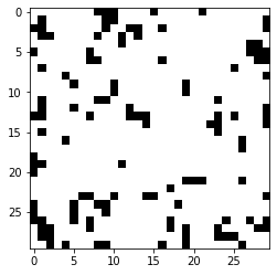
Figure 1: Figures showing that ELBO convergence.

5 Conclusion

In this article, we consider a two-parameter Ising model and proposed a variational Bayes estimation technique. The use of pseudo-likelihood helps to avoid the computation of normalizing constants. The VI procedure facilitates the computation further. We established the theoretical properties of the proposed procedure, which is quite challenging yet needed for statistical validation. The numerical investigation indicates the procedure can work well in applications. There are variations of the Ising models depending on applications. The framework developed in this work will facilitate further developments of this important statistical tool.

Appendix A

A.1 Preliminary notations and Lemmas

Let $\theta=(\beta,B)$. Define $W_{n}=(W_{1n},W_{2n})$

$$W_{1n}(\theta\mid\boldsymbol{x}) =\sum_{i=1}^{n}m_{i}(\boldsymbol{x})\left(x_{i}-\tanh(\beta m_{i}(\boldsymbol{x})+B)\right),$$

$$W_{2n}(\theta\mid\boldsymbol{x}) =\sum_{i=1}^{n}\left(x_{i}-\tanh(\beta m_{i}(\boldsymbol{x})+B)\right),$$ (15)

Define

$$H_{n}(\theta\mid\boldsymbol{x}) =\begin{bmatrix}\sum_{i=1}^{n}m_{i}(\boldsymbol{x})^{2}S_{i}(\theta\mid\boldsymbol{x})&\sum_{i=1}^{n}m_{i}(\boldsymbol{x})S_{i}(\theta\mid\boldsymbol{x})\vspace{2mm}\\ \sum_{i=1}^{n}m_{i}(\boldsymbol{x})S_{i}(\theta\mid\boldsymbol{x})&\sum_{i=1}^{n}S_{i}(\theta\mid\boldsymbol{x})\end{bmatrix}$$ (16)

where $S_{i}(\theta\mid\boldsymbol{x})=\text{sech}^{2}\left(\beta m_{i}(\boldsymbol{x})+B\right)$.

Define

$$R_{1n}(\theta\mid\boldsymbol{x}) :=\begin{bmatrix}\sum_{i=1}^{n}m_{i}(\boldsymbol{x})^{3}\left(h_{i}(\theta\mid\boldsymbol{x})-h_{i}^{3}(\theta\mid\boldsymbol{x})\right)&\sum_{i=1}^{n}m_{i}(\boldsymbol{x})^{2}\left(h_{i}(\theta\mid\boldsymbol{x})-h_{i}^{3}(\theta\mid\boldsymbol{x})\right)\vspace{2mm}\\ \sum_{i=1}^{n}m_{i}(\boldsymbol{x})^{2}\left(h_{i}(\theta\mid\boldsymbol{x})-h_{i}^{3}(\theta\mid\boldsymbol{x})\right)&\sum_{i=1}^{n}m_{i}(\boldsymbol{x})\left(h_{i}(\theta\mid\boldsymbol{x})-h_{i}^{3}(\theta\mid\boldsymbol{x})\right)\end{bmatrix},$$ (17)

and

$$R_{2n}(\theta\mid\boldsymbol{x}) :=\begin{bmatrix}\sum_{i=1}^{n}m_{i}(\boldsymbol{x})^{2}\left(h_{i}(\theta\mid\boldsymbol{x})-h_{i}^{3}(\theta\mid\boldsymbol{x})\right)&\sum_{i=1}^{n}m_{i}(\boldsymbol{x})\left(h_{i}(\theta\mid\boldsymbol{x})-h_{i}^{3}(\theta\mid\boldsymbol{x})\right)\vspace{2mm}\\ \sum_{i=1}^{n}m_{i}(\boldsymbol{x})\left(h_{i}(\theta\mid\boldsymbol{x})-h_{i}^{3}(\theta\mid\boldsymbol{x})\right)&\sum_{i=1}^{n}\left(h_{i}(\theta\mid\boldsymbol{x})-h_{i}^{3}(\theta\mid\boldsymbol{x})\right)\end{bmatrix}.$$ (18)

where $h_{i}(\theta\mid\boldsymbol{x})=\tanh\left(\beta m_{i}(\boldsymbol{x})+B\right)$.

Lemma A.1.

Let $W_{1n}$ and $W_{2n}$ be as in (A.1), then

$$\frac{1}{n}\mathbb{E}_{0}^{(n)}\left(W_{1n}(\theta_{0}\mid\boldsymbol{x})\right)^{2}<\infty\hskip 28.45274pt\frac{1}{n}\mathbb{E}_{0}^{(n)}\left(W_{2n}(\theta_{0}\mid\boldsymbol{x})\right)^{2}<\infty$$

Proof.

See the lemma 2.1 in [11]. ∎

Lemma A.2.

Let $p_{1}$ and $p_{2}$ be any two density functions. Then,

$$\mathbb{E}_{P_{1}}\left(\left|\log\frac{p_{1}}{p_{2}}\right|\right)\leq{\rm KL}(P_{1},P_{2})+\frac{2}{e}$$

Proof.

See the lemma 4 in [19]. ∎

Lemma A.3.

Let $T_{n}(\boldsymbol{x})=\frac{1}{n}\sum_{i=1}^{n}\left(m_{i}(\boldsymbol{x})-\frac{1}{n}\sum_{i=1}^{n}m_{i}(\boldsymbol{x})\right)^{2}$. Suppose Assumptions 1, 2 and 3 hold, then

$$T_{n}(\boldsymbol{x})=O_{p}(1),\hskip 14.22636pt1/T_{n}(\boldsymbol{x})=O_{p}(1)$$

Proof.

See the theorem 1.4 in [11]. ∎

A.2 Taylor expansion for $\log L(\theta)$

Lemma A.4.

Consider the term $(\theta-\theta_{0})^{\top}H_{n}(\theta_{0}\mid\boldsymbol{x})(\theta-\theta_{0})$ where $H_{n}$ is the same as in (16). Then, for some $C_{1},C_{2}>0$, we have

$$\mathbb{P}_{0}^{(n)}\left(C_{1}n\lVert\theta-\theta_{0}\rVert_{2}^{2}\leq(\theta-\theta_{0})^{\top}H_{n}(\theta_{0}\mid\boldsymbol{x})(\theta-\theta_{0})\leq C_{2}n\lVert\theta-\theta_{0}\rVert_{2}^{2}\right)\to 1,n\to\infty$$

Proof.

For some $M_{1},M_{2}>0$, let $\mathcal{A}_{1n}=\{\boldsymbol{x}:T_{n}(\boldsymbol{x})\leq M_{1}\}$, $\mathcal{A}_{2n}=\{\boldsymbol{x}:T_{n}(\boldsymbol{x})\geq M_{2}\}$.

Let $\mathcal{A}_{n}=\mathcal{A}_{1n}\cap\mathcal{A}_{2n}$, then $\mathbb{P}_{0}^{(n)}(\mathcal{A}_{n})\to 1$.

This is because by Lemma A.3, there exists $M_{1}$ and $M_{2}$ such that

$$\mathbb{P}_{0}^{(n)}(T_{n}>M_{1}) =\mathbb{P}_{0}^{(n)}(1/T_{n}<1/M_{1})\to 0$$

$$\mathbb{P}_{0}^{(n)}(T_{n}<M_{2}) =\mathbb{P}_{0}^{(n)}(1/T_{n}>1/M_{2})\to 0$$

The remaining part of the proof works with only $\boldsymbol{x}\in\mathcal{A}_{n}$. Let $e^{H}_{1}\geq e^{H}_{2}$ be the eigenvalues of $H_{n}(\theta_{0}\mid\boldsymbol{x})$. The trace of $H_{n}(\theta_{0}\mid\boldsymbol{x})$, is

$$tr\left(H_{n}(\theta_{0}\mid\boldsymbol{x})\right) =e^{H}_{1}+e^{H}_{2}=\sum_{i=1}^{n}\text{sech}^{2}\left(\beta_{0}m_{i}(\boldsymbol{x})+B_{0}\right)\left(m_{i}^{2}(\boldsymbol{x})+1\right)\leq n(1+\gamma^{2})$$

where we used $|m_{i}(\boldsymbol{x})|\leq\gamma$ based on Assumption 1. Note (2.7) in [11] gives a lower bound of $e^{H}_{2}$:

$$e^{H}_{2}\geq\frac{\text{sech}^{4}(\beta_{0}\gamma+|B_{0}|)}{1+\gamma^{2}}nT_{n}(\boldsymbol{x}),$$ (19)

where $T_{n}(\boldsymbol{x})$ is as in the Lemma A.3. By spectral decomposition of $H_{n}(\theta_{0}\mid\boldsymbol{x})$,

$$(\theta-\theta_{0})^{\top}H_{n}(\theta_{0}\mid\boldsymbol{x})(\theta-\theta_{0}) \leq e^{H}_{1}\left\{(\beta-\beta_{0})^{2}+(B-B_{0})^{2}\right\}$$

$$\leq\left(n(1+\gamma^{2})-e^{H}_{2}\right)\left\{(\beta-\beta_{0})^{2}+(B-B_{0})^{2}\right\}$$

$$\leq n\left((1+\gamma^{2})-\frac{\text{sech}^{4}(\beta_{0}\gamma+|B_{0}|)}{1+\gamma^{2}}T_{n}(\boldsymbol{x})\right)\left\{(\beta-\beta_{0})^{2}+(B-B_{0})^{2}\right\}$$ (20)

Also,

$$(\theta-\theta_{0})^{\top}H_{n}(\theta_{0}\mid\boldsymbol{x})(\theta-\theta_{0}) \geq e^{H}_{2}\left\{(\beta-\beta_{0})^{2}+(B-B_{0})^{2}\right\}$$

$$\geq\frac{\text{sech}^{4}(\beta_{0}\gamma+|B_{0}|)}{1+\gamma^{2}}nT_{n}(\boldsymbol{x})\left\{(\beta-\beta_{0})^{2}+(B-B_{0})^{2}\right\}$$ (21)

Since $M_{2}\leq T_{n}(\boldsymbol{x})\leq M_{1}$ for every $\boldsymbol{x}\in\mathcal{A}_{n}$, the proof follows. ∎

Lemma A.5.

For $R_{1n}$ and $R_{2n}$ as in (17) and (18) respectively, let

$$3R_{n}(\tilde{\theta},\theta-\theta_{0}\mid\boldsymbol{x})$$ (22)

$$=(\beta-\beta_{0})(\theta-\theta_{0})^{\top}R_{1n}(\tilde{\theta}\mid\boldsymbol{x})(\theta-\theta_{0})+(B-B_{0})(\theta-\theta_{0})^{\top}R_{2n}(\tilde{\theta}\mid\boldsymbol{x})(\theta-\theta_{0})$$ (23)

where $R_{n}=R_{n}(\tilde{\theta},\theta-\theta_{0}\mid\boldsymbol{x})$ and $\tilde{\theta}=\theta_{0}+c(\theta-\theta_{0})$ $0<c<1$.

Then, as $n\to\infty$ for some $C_{1},C_{2}>0$ we have

$$\mathbb{P}_{0}^{(n)}(M_{1}n\Delta^{*}\leq R_{n}\leq M_{2}n\Delta^{*})\to 1,\$$

where $\Delta^{*}=((\beta-\beta_{0})\gamma+(B-B_{0}))\lVert\theta_{0}-\theta\rVert_{2}^{2}$

Proof.

For some $M_{1},M_{2}>0$, let $\mathcal{A}_{1n}=\{\boldsymbol{x}:T_{n}(\boldsymbol{x})\leq M_{1}\}$, $\mathcal{A}_{2n}=\{\boldsymbol{x}:T_{n}(\boldsymbol{x})\geq M_{2}\}$.

Let $\mathcal{A}_{n}=\mathcal{A}_{1n}\cap\mathcal{A}_{2n}$, then $\mathbb{P}_{0}^{(n)}(\mathcal{A}_{n})\to 1$.

This is because by Lemma A.3, there exists $M_{1},M_{2}>0$ such that

$$\mathbb{P}_{0}^{(n)}(T_{n}>M_{1}) =\mathbb{P}_{0}^{(n)}(1/T_{n}<1/M_{1})\to 0$$

$$\mathbb{P}_{0}^{(n)}(T_{n}<M_{2}) =\mathbb{P}_{0}^{(n)}(1/T_{n}>1/M_{2})\to 0$$

The remaining part of the proof works with only $\boldsymbol{x}\in\mathcal{A}_{n}$.

The determinant of $R_{1n}(\tilde{\theta}\mid\boldsymbol{x})$ is:

$$det(R_{1n}(\tilde{\theta}\mid\boldsymbol{x}))$$

$$=\frac{1}{2}\sum_{i,j=1}^{n}m_{i}(\boldsymbol{x})m_{j}(\boldsymbol{x})\left(h_{i}(\boldsymbol{x})-h_{i}^{3}(\boldsymbol{x})\right)\left(h_{j}(\boldsymbol{x})-h_{j}^{3}(\boldsymbol{x})\right)\left(m_{i}(\boldsymbol{x})-m_{j}(\boldsymbol{x})\right)^{2}$$

where $h_{i}(\boldsymbol{x})=\tanh(\tilde{\beta}m_{i}(\boldsymbol{x})+\tilde{B})$. Since $\tanh(\cdot)-\tanh^{3}(\cdot)$ has maximum value $0.38$ at $\sqrt{3}/{3}$ and $m_{i}(\boldsymbol{x})\leq\gamma$ by Assumption 1. Therefore,

$$|det(R_{1n}(\tilde{\theta}\mid\boldsymbol{x}))| \leq\frac{1}{2}\gamma^{2}(0.38)^{2}\sum_{i=1}^{n}\sum_{j=1}^{n}\left(m_{i}(\boldsymbol{x})-m_{j}(\boldsymbol{x})\right)^{2}=\gamma^{2}(0.38)^{2}n^{2}T_{n}(\boldsymbol{x}).$$

The trace of $R_{1n}(\tilde{\theta}\mid\boldsymbol{x})$ is:

$$tr(R_{1n}(\tilde{\theta}\mid\boldsymbol{x})) =\sum_{i=1}^{n}m_{i}(\boldsymbol{x})(h_{i}(\boldsymbol{x})-h_{i}^{3}(\boldsymbol{x}))\left(m_{i}^{2}(\boldsymbol{x})+1\right)\leq n0.38\gamma(1+\gamma^{2}).$$

Let $e_{1}^{R_{1n}}\geq e_{2}^{R_{1n}}$ be eigenvalues of $R_{1n}(\tilde{\theta}\mid\boldsymbol{x})$.

$$e_{2}^{R_{1n}} \geq\frac{e_{1}^{R_{1n}}e_{2}^{R_{1n}}}{e_{1}^{R_{1n}}+e_{2}^{R_{1n}}}=\frac{det(R_{1n}(\tilde{\theta}\mid\boldsymbol{x}))}{tr(R_{1n}(\tilde{\theta}\mid\boldsymbol{x}))} \geq-\frac{\gamma^{2}(0.38)^{2}n^{2}T_{n}(\boldsymbol{x})}{n0.38\gamma(1+\gamma^{2})}=-\frac{0.38\gamma}{1+\gamma^{2}}nT_{n}(\boldsymbol{x}).$$

Therefore,

$$(\theta-\theta_{0})^{\top}R_{1n}(\tilde{\theta}\mid\boldsymbol{x})(\theta-\theta_{0}) \geq e_{2}^{R_{1n}}||\theta-\theta_{0}||_{2}^{2}\geq-\frac{0.38\gamma}{1+\gamma^{2}}nT_{n}(\boldsymbol{x})||\theta-\theta_{0}||_{2}^{2}$$ (24)

and

$$(\theta-\theta_{0})^{\top}R_{1n}(\tilde{\theta}\mid\boldsymbol{x})(\theta-\theta_{0}) \leq e_{1}^{R_{1n}}||\theta-\theta_{0}||_{2}^{2}=(tr(R_{1n}(\tilde{\theta}\mid\boldsymbol{x}))-e_{2}^{R_{1n}}))||\theta-\theta_{0}||_{2}^{2}$$

$$\leq 0.38\gamma n\left((1+\gamma^{2})+\frac{T_{n}(\boldsymbol{x})}{1+\gamma^{2}}\right)||\theta-\theta_{0}||_{2}^{2}.$$ (25)

With the same argument, we can get:

$$(\theta-\theta_{0})^{\top}R_{2n}(\tilde{\theta}\mid\boldsymbol{x})(\theta-\theta_{0}) \geq-\frac{0.38}{1+\gamma^{2}}nT_{n}(\boldsymbol{x})||\theta-\theta_{0}||_{2}^{2},$$ (26)

$$(\theta-\theta_{0})^{t}R_{2n}(\tilde{\theta}\mid\boldsymbol{x})(\theta-\theta_{0}) \leq 0.38n\left((1+\gamma^{2})+\frac{T_{n}(\boldsymbol{x})}{1+\gamma^{2}}\right)||\theta-\theta_{0}||_{2}^{2}$$ (27)

Using (24), (A.5), (26) and (27) and noting $M_{2}\leq T_{n}(\boldsymbol{x})\leq M_{1}$ for every $\boldsymbol{x}\in\mathcal{A}_{n}$, the proof follows. ∎

Lemma A.6.

Let $q(\theta)\in\mathcal{Q}^{MF}$ with $\mu_{1}=\log\beta_{0}$, $\mu_{2}=B_{0}$, and $\sigma_{1}^{2}=\sigma_{2}^{2}=1/n$, then

$$\frac{1}{n\epsilon_{n}^{2}\log n}{\rm KL}(Q,P)\to 0,\>\>n\to\infty$$

Proof.

Using the same notation in (5), the first term is:

$${\rm KL}(Q,P) =\mathbb{E}_{q_{\beta}(\beta)q_{B}(B)}\left(\log q_{\beta}(\beta)+\log q_{B}(B)-\log p_{\beta}(\beta)-\log p_{B}(B)\right)$$

$$={\rm KL}\left(Q_{\beta},P_{\beta}\right)+{\rm KL}\left(Q_{B},P_{B}\right)$$

$$=\frac{1}{2}\left((\log\beta_{0})^{2}+\frac{1}{n}+B_{0}^{2}+\frac{1}{n}-2\right)+\log n=o(n\epsilon_{n}^{2}\log n),\>\>\>\>\text{since $n\epsilon_{n}^{2}\to\infty$}$$

∎

A.3 Technical details of Lemma 3.2

Proof of Lemma 3.2.

Let $\mathcal{V}_{\epsilon_{n}}=\{|\beta-\beta_{0}|<\epsilon_{n},|B-B_{0}|<\epsilon_{n}\}$. Then $\mathcal{V}_{\epsilon_{n}}\subseteq\mathcal{U}_{\sqrt{2}\epsilon_{n}}$ which implies $\mathcal{U}_{\sqrt{2}\epsilon_{n}}^{c}\subseteq\mathcal{V}_{\epsilon_{n}}^{c}$ which further implies

$$\log\int_{\mathcal{U}_{\sqrt{2}\epsilon_{n}}^{c}}\frac{L(\theta)}{L(\theta_{0})}p(\theta)d\theta\leq\log\int_{\mathcal{V}_{\epsilon_{n}}^{c}}\frac{L(\theta)}{L(\theta_{0})}p(\theta)d\theta$$ (28)

We shall now establish for some $C_{0}>0$

$$\mathbb{P}_{0}^{(n)}\left(\log\int_{\mathcal{V}_{\epsilon_{n}}^{c}}\frac{L(\theta)}{L(\theta_{0})}p(\theta)d\theta\leq-C_{0}n\epsilon_{n}^{2}\right) \to 1,\>\>n\to\infty,$$

which in lieu of (28) completes the proof.

Define $\mathcal{A}_{1n}=\{\boldsymbol{x}:W_{1n}(\theta_{0}\mid\boldsymbol{x})^{2}+W_{1n}(\theta_{0}\mid\boldsymbol{x})^{2}\leq n^{2/3}\}$ and $\mathcal{A}_{2n}=\{\boldsymbol{x}:T_{n}(\boldsymbol{x})\geq M\}$ for some $M>0$. Define $\mathcal{A}_{n}=\mathcal{A}_{1n}\cap\mathcal{A}_{2n}$.

Here $\mathbb{P}_{0}^{(n)}(\mathcal{A}_{n})\to 1$. This because by Markov’s inequality and Lemma A.1,

$$\mathbb{P}_{0}^{(n)}\left(W_{1n}(\theta_{0}\mid\boldsymbol{x})^{2}+W_{2n}(\theta_{0}\mid\boldsymbol{x})^{2}>n^{2/3}\varepsilon\right)$$

$$\leq\frac{1}{n^{4/3}}\mathbb{E}_{0}^{(n)}\left(W_{1n}(\theta_{0}\mid\boldsymbol{x})^{2}+W_{2n}(\theta_{0}\mid\boldsymbol{x})^{2}\right)\to 0.$$

and by Lemma A.3 $\mathbb{P}_{0}^{(n)}(T_{n}<M)=\mathbb{P}_{0}^{(n)}(1/T_{n}>1/M)\to 0$.

We shall show for $\boldsymbol{x}\in\mathcal{A}_{n}$, $L(\theta)/L(\theta_{0})\leq e^{-C_{0}n\epsilon_{n}^{2}}$, $\forall$ $\theta\in\mathcal{V}_{\epsilon_{n}}^{c}$ which implies $\forall$ $\boldsymbol{x}\in\mathcal{A}_{n}$,

$$\log\int_{\mathcal{V}_{\epsilon_{n}}^{c}}(L(\theta)/L(\theta_{0}))p(\theta)d\theta =\log\int_{\mathcal{V}_{\epsilon_{n}}^{c}}(L(\theta)/L(\theta_{0}))p(\theta)d\theta$$

$$\leq\log(e^{-C_{0}n\epsilon_{n}^{2}}\int_{\mathcal{V}_{\epsilon_{n}}^{c}}p(\theta)d\theta)\leq-C_{0}n\epsilon_{n}^{2}$$ (29)

since $p(\mathcal{V}_{\epsilon_{n}^{c}})\leq 1$. This completes the proof since $\mathbb{P}_{0}^{(n)}(\mathcal{A}_{n})\to 1$ as $n\to\infty$.

Next, note that $\mathcal{V}_{\epsilon_{n}}^{c}$ is given by the union of the following terms

$$V_{1n} =\{(\beta,B):\beta-\beta_{0}\geq\epsilon_{n},B\geq B_{0}\},V_{2n}=\{(\beta,B):\beta-\beta_{0}\geq\epsilon_{n},B<B_{0}\}$$

$$V_{3n} =\{(\beta,B):\beta-\beta_{0}<-\epsilon_{n},B\geq B_{0}\},V_{4n}=\{(\beta,B):\beta-\beta_{0}<-\epsilon_{n},B<B_{0}\}$$

$$V_{5n} =\{(\beta,B):\beta\geq\beta_{0},B-B_{0}\geq\epsilon_{n}\},V_{6n}=\{(\beta,B):\beta<\beta_{0},B-B_{0}\geq\epsilon_{n}\}$$

$$V_{7n} =\{(\beta,B):\beta\geq\beta_{0},B-B_{0}<-\epsilon_{n}\},V_{8n}=\{(\beta,B):\beta<\beta_{0},B-B_{0}<-\epsilon_{n}\}$$

We shall now show for $\boldsymbol{x}\in\mathcal{A}_{n}$ and $\theta\in V_{1n}$, $L(\theta)/L(\theta_{0})\leq e^{-C_{0}n\epsilon_{n}^{2}}$. The proof of other parts follow similarly.

(a) Let $\theta=(\beta,B)$ and $\theta_{0}^{\prime}=(\beta_{0}+\epsilon,B_{0})$, where $\beta\geq\beta_{0}+\epsilon$ and $B\geq B_{0}$. Also, define

$$\theta_{t}=\theta_{0}^{\prime}+t(\theta-\theta_{0}^{\prime})~{}\text{where}~{}0<t<1.$$

Consider a function $g$:

$$g(t)=f(\theta_{t})=\log L(\theta_{t})-\log L(\theta_{0}^{\prime})-\Delta_{n}(\theta_{0}^{\prime})^{\top}(\theta_{t}-\theta_{0}^{\prime}),$$

where $\Delta_{n}(\theta)=\left(\nabla_{\beta}\log L(\theta),\nabla_{B}\log L(\theta)\right)^{\top}$. Note that $g(t)$ is a function of $t$. We want to show $g(t)\leq g(0)$ provided $t>0$. We shall instead show $g^{\prime}(t)\leq 0$. By Taylor expansion,

$$g^{\prime}(t)=g^{\prime}(0)+g^{\prime\prime}(\tilde{t})t.$$

for some $\tilde{t}\in[0,t]$. Here, $g^{\prime}(0)=0$ and $g^{\prime\prime}(\tilde{t})=-(\theta-\theta_{0}^{\prime})^{\top}H_{n}(\theta_{\tilde{t}}\mid\boldsymbol{x})(\theta-\theta_{0}^{\prime})\leq 0$ where $H_{n}$ as in (16) is a positive definite matrix (by (A.4) in A.4 and $T_{n}(\boldsymbol{x})\geq 0$). Since $g(t)$ is decreasing for $0<t<1$, thus

$$g(1)\leq g(0)\implies f(\theta)\leq f(\theta_{0}^{\prime})$$

(b) Similarly, let $\theta=(\beta,B)$ $\theta_{0}^{\prime\prime}=(\beta_{0},B_{0}+\epsilon)$, where $\beta\geq\beta_{0}$ and $B\geq B_{0}+\epsilon$. Define

$$\theta_{t}=\theta_{0}^{\prime}+t(\theta-\theta_{0}^{\prime\prime})~{}\text{where}~{}0<t<1.$$

$$h(t)=f(\theta_{t})=\log L(\theta_{t})-\log L(\theta_{0}^{\prime\prime})-\Delta_{n}(\theta_{0}^{\prime\prime})^{\top}(\theta_{t}-\theta_{0}^{\prime\prime}).$$

With similar argument in (a), we conclude that $h(1)\leq h(0)\implies f(\theta)\leq f(\theta_{0}^{\prime\prime})$. Therefore,

$$\sup_{\theta\in V_{1n}}(\log L(\theta)-\log L(\theta_{0}))$$

$$\leq\sup_{\{\beta-\beta_{0}\in[\epsilon_{n},\epsilon],B\geq B_{0}\}}(\log L(\theta)-\log L(\theta_{0}))+\sup_{\{\beta>\beta_{0}+\epsilon,B\geq B_{0}\}}(\log L(\theta)-\log L(\theta_{0}))$$

$$\leq\sup_{\{\beta-\beta_{0}\in[\epsilon_{n},\epsilon],B\geq B_{0}\}}(\log L(\theta)-\log L(\theta_{0}))+(\log L(\theta_{0}^{\prime})-\log L(\theta_{0}))$$

$$\leq\sup_{\{\beta-\beta_{0}\in[\epsilon_{n},\epsilon],B-B_{0}\in[0,\epsilon]\}}(\log L(\theta)-\log L(\theta_{0}))+\sup_{\{\beta-\beta_{0}\in[\epsilon_{n},\epsilon],B>B_{0}+\epsilon\}}(\log L(\theta)-\log L(\theta_{0}))$$

$$+\log L(\theta_{0}^{\prime})-\log L(\theta_{0}))$$

$$\leq\sup_{\{\beta-\beta_{0}\in[\epsilon_{n},\epsilon],B-B_{0}\in[0,\epsilon]\}}(\log L(\theta)-\log L(\theta_{0}))+\sup_{\{\beta\geq\beta_{0},B>B_{0}+\epsilon\}}(\log L(\theta)-\log L(\theta_{0}))$$

$$+\log L(\theta_{0}^{\prime})-\log L(\theta_{0}))$$

$$\leq\sup_{\{\beta-\beta_{0}\in[\epsilon_{n},\epsilon],B-B_{0}\in[0,\epsilon]\}}(\log L(\theta)-\log L(\theta_{0}))+\log L(\theta_{0}^{\prime\prime})-\log L(\theta_{0})$$

$$+\log L(\theta_{0}^{\prime})-\log L(\theta_{0})$$

$$\leq\sup_{\{\beta-\beta_{0}\in[\epsilon_{n},\epsilon],B-B_{0}\in[0,\epsilon]\}}3(\log L(\theta)-\log L(\theta_{0}))\leq-C_{0}n\epsilon_{n}^{2}$$ (30)

where the second inequality follows from (a) and fifth inequality follows from (b) above. Finally for the last inequality, consider Taylor expansion for $\log L(\theta)$ upto the second order

$$\log L(\theta)-\log L(\theta_{0}) =W_{n}(\theta_{0}\mid\boldsymbol{x})^{\top}(\theta-\theta_{0})-\frac{1}{2}(\theta-\theta_{0})^{\top}H_{n}(\tilde{\theta}\mid\boldsymbol{x})(\theta-\theta_{0})$$

where $\tilde{\theta}=\theta_{0}+c(\theta-\theta_{0})$, $0<c<1$ and $W_{n}$ and $H_{n}$ are as defined in (A.1) and (16) respectively.

By Cauchy Schwarz inequality,

$$|W_{n}(\theta_{0}\mid\boldsymbol{x})^{\top}(\theta-\theta_{0}))| \leq(\left(W_{1n}(\theta_{0}\mid\boldsymbol{x})^{2}+W_{2n}(\theta_{0}\mid\boldsymbol{x})^{2}\right)\lVert\theta-\theta_{0}\rVert_{2}^{2}+1)$$

$$\leq n^{2/3}\lVert\theta-\theta_{0}\rVert_{2}^{2}+1$$

for every $\boldsymbol{x}\in\mathcal{A}_{n}$. Further

$$\log L(\theta)-\log L(\theta_{0}) \leq n^{2/3}\lVert\theta-\theta_{0}\rVert_{2}^{2}+1-\frac{1}{2}(\theta-\theta_{0})^{\top}H_{n}(\tilde{\theta}\mid\boldsymbol{x})(\theta-\theta_{0})$$

$$\leq n^{2/3}\lVert\theta-\theta_{0}\rVert_{2}^{2}+1-\frac{\text{sech}^{4}(\tilde{\beta}\gamma+|\tilde{B}|)}{1+\gamma^{2}}nT_{n}(\boldsymbol{x})\lVert\theta-\theta_{0}\rVert_{2}^{2}$$

$$\leq\left(n^{2/3}+\frac{1}{||\theta-\theta_{0}||_{2}^{2}}-\frac{\text{sech}^{4}(\tilde{\beta}\gamma+|\tilde{B}|)}{1+\gamma^{2}}\frac{n}{M}\right)\lVert\theta-\theta_{0}\rVert_{2}^{2}$$

where the second inequality is a consequence of the lower bound (19) and the third inequality holds since $\boldsymbol{x}\in\mathcal{A}_{n}$. Taking $\sup$ over the set $\{\beta-\beta_{0}\in[\epsilon_{n},\epsilon],B-B_{0}\in[0,\epsilon]\}$ on both sides,

$$\sup_{\{\beta-\beta_{0}\in[\epsilon_{n},\epsilon],B-B_{0}\in[0,\epsilon]\}}(\log L(\theta)-\log L(\theta_{0}))$$

$$\leq\sup_{\{\beta-\beta_{0}\in[\epsilon_{n},\epsilon],B-B_{0}\in[0,\epsilon]\}}\left(n^{2/3}+\frac{1}{\epsilon_{n}^{2}}-\frac{\text{sech}^{4}((\beta_{0}+\epsilon)\gamma+(B_{0}+\epsilon))}{1+\gamma^{2}}\frac{n}{M}\right)\lVert\theta-\theta_{0}\rVert_{2}^{2}$$

$$\leq-C_{0}n\epsilon_{n}^{2}$$ (31)

for some $C_{0}>0$ as $n\to\infty$ since $n^{2/3}$ and $1/\epsilon_{n}^{2}=o(n)$.This completes the proof. ∎

A.4 Technical details of Lemma 3.3

Lemma A.7.

Let $L_{0}$ and $L(\theta_{0})$ represent the true likelihood (1) and the pseudo-likelihood (2.2) with the true parameters, respectively. Then,

$$\frac{1}{n\epsilon_{n}^{2}}\mathbb{E}_{0}^{(n)}(\log L_{0}-\log L(\theta_{0}))\to 0,\>\>n\to\infty$$

Proof.

$$L_{0}=\frac{e^{f_{\theta_{0}}(\boldsymbol{x})}}{\sum_{\boldsymbol{x}\in\{-1,1\}^{n}}e^{f_{\theta_{0}}(\boldsymbol{x})}}=\frac{e^{f_{\theta_{0}}(\boldsymbol{x})}}{Z_{n}(\theta_{0})}$$

where $f_{\theta_{0}}(\boldsymbol{x})=(\beta_{0}/2)\boldsymbol{x}^{\top}A_{n}\boldsymbol{x}+B_{0}\boldsymbol{x}^{\top}1$. Define $b(\boldsymbol{x};\theta)=(b_{1}(\boldsymbol{x};\theta),\cdots,b_{n}(\boldsymbol{x};\theta))$ where

$$b_{i}(\boldsymbol{x};\theta)=E(X_{i}|X_{j},j\neq i)=\tanh(\beta m_{i}(\boldsymbol{x})+B)$$

Then $L(\theta)=e^{g(\boldsymbol{x},b(\boldsymbol{x};\theta))}$ where the function $g$ for $\boldsymbol{v},\boldsymbol{w}\in[-1,1]^{n}$ is defined as

$$g(\boldsymbol{v},\boldsymbol{w})=\sum_{i=1}^{n}\frac{1+v_{i}}{2}\log\frac{1+w_{i}}{2}+\frac{1-v_{i}}{2}\log\frac{1-w_{i}}{2}$$

Also, define $I(\boldsymbol{v})=g(\boldsymbol{v},\boldsymbol{v})$. Now, observe that

$$\mathbb{E}_{0}^{(n)}(\log L_{0}-\log L(\theta_{0})) =\mathbb{E}_{0}^{(n)}(f_{\theta_{0}}(\boldsymbol{x})-g(\boldsymbol{x},b(\boldsymbol{x};\theta_{0}))-\log Z_{n}(\theta_{0}))$$

$$=\mathbb{E}_{0}^{(n)}(f_{\theta_{0}}(\boldsymbol{x})-f_{\theta_{0}}(b(\boldsymbol{x};\theta_{0}))+\mathbb{E}_{0}^{(n)}(f_{\theta_{0}}(b(\boldsymbol{x};\theta_{0}))-I(b(\boldsymbol{x};\theta_{0})))$$

$$+\mathbb{E}_{0}^{(n)}(I(b(\boldsymbol{x};\theta_{0}))-g(x,b(\boldsymbol{x};\theta_{0})))-\log Z_{n}(\theta_{0})$$

$$\leq(\mathbb{E}_{0}^{(n)}(f_{\theta_{0}}(\boldsymbol{x})-f_{\theta_{0}}(b(\boldsymbol{x};\theta_{0})))^{2})^{1/2}+(\mathbb{E}_{0}^{(n)}(I(b(\boldsymbol{x};\theta_{0}))-g(\boldsymbol{x},b(\boldsymbol{x};\theta_{0})))^{2})^{1/2}$$

$$+\mathbb{E}_{0}^{(n)}(f_{\theta_{0}}(b(\boldsymbol{x};\theta_{0}))-I(b(\boldsymbol{x};\theta_{0})))-\log Z_{n}(\theta_{0}),$$ (32)

where the last step is due to Hölder’s inequality.

Under Assumption 2, mimicking the proof of Lemmas 3.2 and 3.3 in [2] with $n$ replaced by $n\epsilon_{n}^{2}$, we get

$$(\mathbb{E}_{0}^{(n)}(f_{\theta_{0}}(\boldsymbol{x})-f_{\theta_{0}}(b(\boldsymbol{x};\theta_{0})))^{2})^{1/2}=o(n\epsilon_{n}^{2})$$ (33)

$$(\mathbb{E}_{0}^{(n)}(I(b(\boldsymbol{x};\theta_{0}))-g(\boldsymbol{x},b(\boldsymbol{x};\theta_{0})))^{2})^{1/2}=o(n\epsilon_{n}^{2})$$ (34)

Also for $r_{n}=\sup_{\boldsymbol{v}\in{[-1,1]}^{n}}(f_{\theta_{0}}(\boldsymbol{v})-I(\boldsymbol{v}))$, we have

$$\mathbb{E}_{0}^{(n)}(f_{\theta_{0}}(b(\boldsymbol{x},\theta_{0}))-I(b(\boldsymbol{x},\theta_{0})))\leq r_{n}$$

By Theorem 1.6 in [7] with the fact $\partial^{2}f_{\theta_{0}}/\partial x_{i}^{2}=0$, $i=1,\cdots,n$, we have $-\log Z_{n}(\theta_{0})\leq-r_{n}$. Therefore,

$$\mathbb{E}_{0}^{(n)}(f_{\theta_{0}}(b(\boldsymbol{x};\theta_{0}))-I(b(\boldsymbol{x};\theta_{0}))-\log Z_{n}(\theta_{0}))\leq 0.$$ (35)

Using (33), (34) and (35) in (A.4) completes the proof. ∎

Lemma A.8.

Note that $L(\theta)$ is not a valid density function. So, we consider $\tilde{L}(\theta)=L(\theta)/J_{n}(\theta)$ where $J_{n}(\theta)=\sum_{\boldsymbol{x}\in\{-1,1\}^{n}}L(\theta)$ such that $\sum_{\boldsymbol{x}\in\{-1,1\}^{n}}\tilde{L}(\theta)=1$. Then for every $\theta$,

$$J_{n}(\theta)\leq\beta\epsilon_{n}\sqrt{n(1+\gamma^{2})/2}+o(n\epsilon_{n}^{2})(\log 3\sqrt{2}-\log\epsilon_{n}).$$

Proof.

Let $N_{n}(\epsilon_{n}):=\{i\in[n]:|\lambda_{i}(A_{n})|>\epsilon_{n}/\sqrt{2}\}$ and with the mean field condition in the Assumption 2, it is easy to note that

$$\frac{\left|N_{n}(\epsilon_{n})\right|}{n}\leq\frac{2}{n\epsilon_{n}^{2}}\sum_{i\in[n]}\lambda_{i}\left(A_{n}\right)^{2}=\frac{2}{n\epsilon_{n}^{2}}\sum_{i,j=1}^{n}A_{n}(i,j)^{2}\rightarrow 0,\>\>n\rightarrow\infty$$ (36)

Set $k_{n}=|N_{n}(\epsilon_{n})|$ and let $D_{n,0}(\epsilon_{n})$ be a $\epsilon_{n}\sqrt{n/2}$ net of the set $\{\boldsymbol{f}\in\mathbb{R}^{k_{n}}:\sum f_{i}^{2}\leq n\}$ of size at most $(3\sqrt{2}/\epsilon_{n})^{k_{n}}$. The existence of such a net is standard (see for example Lemma 2.6 in [23]).

Let $\{\boldsymbol{p}_{1},\cdots,\boldsymbol{p}_{n}\}$ be the eigen vectors of $A_{n}$. Then setting

$$D_{n,1}(\epsilon_{n}):=\{\sum_{i\in N_{n}(\epsilon_{n})}c_{i}\lambda_{i}(A_{n})\boldsymbol{p}_{i},\boldsymbol{c}\in D_{n,0}(\epsilon_{n})\}$$

We claim $D_{n,1}(\epsilon_{n})$ is $\epsilon_{n}\sqrt{n(1+\gamma^{2})/2}$ of the set $\{A_{n}\boldsymbol{x}:\boldsymbol{x}\in\{-1,1\}^{n}\}$. Indeed any $\boldsymbol{x}\in\{-1,1\}^{n}$ can be written as $\sum_{i=1}^{n}f_{i}\boldsymbol{p}_{i}$ where $\sum_{i=1}^{n}f_{i}^{2}=\sum x_{i}^{2}=n$. In particular, it means $\sum_{i\in N_{n}(\epsilon_{n})}f_{i}\leq n$, which implies there exists a $\boldsymbol{c}\in D_{n,0}(\epsilon_{n})$ such that $||\boldsymbol{c}-\boldsymbol{f}||\leq\epsilon_{n}\sqrt{n/2}$.

Let $\sum_{i\in N_{n}(\epsilon_{n})}c_{i}\lambda_{i}(A_{n})\boldsymbol{p}_{i}\in D_{n,1}(\epsilon_{n})$, then

$$||A_{n}\boldsymbol{x}-\sum_{i\in N_{n}(\epsilon_{n})}c_{i}\lambda_{i}(A_{n})\boldsymbol{p}_{i}||_{2}^{2} =\sum_{i\in N_{n}(\epsilon_{n})}(c_{i}-f_{i})^{2}\lambda_{i}(A_{n})^{2}+\sum_{i\notin N_{n}(\epsilon_{n})}\lambda_{i}(A_{n})^{2}f_{i}^{2}$$

$$\leq\frac{\gamma^{2}n\epsilon_{n}^{2}}{2}+\frac{n\epsilon_{n}^{2}}{2}$$

where the last inequality is a consequence of $\max_{i\in[n]}|\lambda_{i}(A_{n})|\leq\max_{i\in[n]}\sum_{j=1}^{n}|A_{n}(i,j)|\leq\gamma$ and the definition of the set $N_{n}(\epsilon_{n})$.

In particular for any $\boldsymbol{x}\in\{-1,1\}^{n}$, there exists at least one $\boldsymbol{p}\in D_{n,1}(\epsilon_{n})$ such that $||\boldsymbol{p}-m(\boldsymbol{x})||\leq\epsilon_{n}\sqrt{n(1+\gamma^{2})/2}$. For any $\boldsymbol{p}\in D_{n,1}(\epsilon_{n})$, let

$$\mathcal{P}(\boldsymbol{p}):=\{\boldsymbol{x}\in\{-1,1\}^{n}:||\boldsymbol{p}-m(\boldsymbol{x})||\leq\epsilon_{n}\sqrt{n(1+\gamma^{2})/2}\}$$

Therefore,

$$\sum_{\boldsymbol{x}\in\{-1,1\}^{n}}e^{g(\boldsymbol{x},b(\boldsymbol{x};\theta))}=\sum_{\boldsymbol{p}\in D_{n,1}(\epsilon_{n})}\sum_{\boldsymbol{x}\in\mathcal{P}(\boldsymbol{p})}e^{g(\boldsymbol{x},b(\boldsymbol{x};\theta))}$$

Setting $\boldsymbol{u}(\boldsymbol{p}):=\tanh(\beta\boldsymbol{p}+B)$ if $||\boldsymbol{p}-m(\boldsymbol{x})||\leq\epsilon_{n}\sqrt{n(1+\gamma^{2})/2}$, then we have

$$|g(\boldsymbol{x},b(\boldsymbol{x};\theta))-g(\boldsymbol{x},\boldsymbol{u}(\boldsymbol{p}))|\leq 2\beta\sum_{i=1}^{n}|m_{i}(\boldsymbol{x})-p_{i}|\leq 2\beta\epsilon_{n}\sqrt{n(1+\gamma^{2})/2}$$

Finally,

$$\sum_{\boldsymbol{x}\in\{-1,1\}^{n}}e^{g(\boldsymbol{x},b(\boldsymbol{x};\theta))} \leq e^{\beta\sqrt{n}\epsilon_{n}}\sum_{\boldsymbol{p}\in D_{n,1}(\epsilon_{n})}\sum_{\boldsymbol{x}\in\mathcal{P}(\boldsymbol{p})}e^{g(\boldsymbol{x},u(\boldsymbol{p}))}$$

$$\leq e^{\beta\sqrt{n}\epsilon_{n}}\sum_{\boldsymbol{p}\in D_{n,1}(\epsilon_{n})}\sum_{\boldsymbol{x}\in\{-1,1\}^{n}}e^{g(\boldsymbol{x},u(\boldsymbol{p}))}=e^{\beta\epsilon_{n}\sqrt{n(1+\gamma^{2})/2}}|D_{n,1}(\epsilon_{n})|$$

where the last equality follows since $\sum_{\boldsymbol{x}\in\{-1,1\}^{n}}e^{g(x,u)}=1$ for any $u\in[-1,1]^{n}$. Therefore,

$$\log J_{n}(\theta)\leq\beta\epsilon_{n}\sqrt{n(1+\gamma^{2})/2}+\log|D_{n,1}(\epsilon_{n})|$$

Since $|D_{n,1}(\epsilon_{n})|=|D_{n,0}(\epsilon_{n})|$, therefore

$$\log|D_{n,1}(\epsilon_{n})|\leq|N_{n}(\epsilon_{n})|(\log 3\sqrt{2}-\log\epsilon_{n})$$

The proof follows since $|N_{n}(\epsilon_{n})|=o(n\epsilon_{n}^{2})$. ∎

Lemma A.9.

Define $\mathcal{V}_{\epsilon_{n}}:=\{\theta:|\beta-\beta_{0}|<\epsilon_{n},|B-B_{0}|<\epsilon_{n}\}$. Then,

$$\mathcal{V}_{\epsilon_{n}}\subseteq\mathcal{K}_{\epsilon_{n}},\>\>\text{for $n$ sufficiently large}$$

where $\mathcal{K}_{\epsilon_{n}}:=\{\theta:\mathbb{E}_{0}^{(n)}(\log(L(\theta_{0})/L(\theta)))<3n\epsilon_{n}^{2}\}$.

Proof.

For any $\theta\in\mathcal{V}_{\epsilon_{n}}$, using the decomposition in (A.5), we get

$$\mathbb{E}_{0}^{(n)}\left(\log L(\theta_{0})-\log L(\theta)\right) =\mathbb{E}_{0}^{(n)}\left(-\leavevmode\hbox to14.18pt{\vbox to14.18pt{\text{[drawing]}}}-\leavevmode\hbox to14.18pt{\vbox to14.18pt{\text{[drawing]}}}+\leavevmode\hbox to14.18pt{\vbox to14.18pt{\text{[drawing]}}}-\leavevmode\hbox to14.18pt{\vbox to14.18pt{\text{[drawing]}}}\right)\leq 3n\epsilon_{n}^{2}$$

where the last inequality is justified next.

For some $M>0$ using Lemma A.1, we get

$$-\mathbb{E}_{0}^{(n)}(\leavevmode\hbox to14.18pt{\vbox to14.18pt{\text{[drawing]}}}) =(\beta_{0}-\beta)\mathbb{E}_{0}^{(n)}(W_{1n}(\theta_{0}|\boldsymbol{x})\leq\sqrt{n}|\beta_{0}-\beta|\left(\frac{1}{n}\mathbb{E}_{0}^{(n)}\left(W_{1n}(\theta_{0}|\boldsymbol{x})\right)^{2}\right)^{1/2}$$

$$\leq M\sqrt{n}\epsilon_{n}$$

$$-\mathbb{E}_{0}^{(n)}(\leavevmode\hbox to14.18pt{\vbox to14.18pt{\text{[drawing]}}}) =(B_{0}-B)\mathbb{E}_{0}^{(n)}(W_{2n}(\theta_{0}|\boldsymbol{x})\leq\sqrt{n}|B_{0}-B|\left(\frac{1}{n}\mathbb{E}_{0}^{(n)}\left(W_{2n}(\theta_{0}|\boldsymbol{x})\right)^{2}\right)^{1/2}$$

$$\leq M\sqrt{n}\epsilon_{n}$$

By relation (A.4), we get

$$\mathbb{E}_{0}^{(n)}(\leavevmode\hbox to14.18pt{\vbox to14.18pt{\text{[drawing]}}})\leq n||\theta-\theta_{0}||_{2}^{2}\left((1+\gamma^{2})-\frac{\text{sech}^{4}(\beta_{0}\gamma+|B_{0}|)}{1+\gamma^{2}}\mathbb{E}_{0}^{(n)}\left(T_{n}(\boldsymbol{x})\right)\right)\leq 2(1+\gamma^{2})n\epsilon_{n}^{2}$$

By relation (43), we get

$$-\mathbb{E}_{0}^{(n)}(\leavevmode\hbox to14.18pt{\vbox to14.18pt{\text{[drawing]}}})\leq\frac{0.38n}{3(1+\gamma^{2})}\mathbb{E}_{0}^{(n)}\left(T_{n}(\boldsymbol{x})\right)||\theta-\theta_{0}||_{2}^{2}(|\beta-\beta_{0}|\gamma+|B-B_{0}|)\leq\frac{0.38\gamma^{2}(1+\gamma)}{3(1+\gamma^{2})}n\epsilon_{n}^{3}$$

∎

Lemma A.10.

With prior distribution $p(\theta)$ as in (3), we have

$$\int_{\mathcal{V}_{\epsilon_{n}}}p(\theta)d\theta\geq C\epsilon_{n}^{2},\hskip 14.22636pt\text{for some $C>0$}$$

Proof.

By mean value theorem with $\beta^{\star}\in[\beta_{0}-\epsilon_{n},\beta_{0}+\epsilon_{n}]$ and $B^{\star}\in[B_{0}-\epsilon_{n},B_{0}+\epsilon_{n}]$,

$$\int_{V_{\epsilon_{n}}}p(\theta)d\theta =\int_{\beta_{0}-\epsilon}^{\beta_{0}+\epsilon}\frac{1}{\beta\sqrt{2\pi}}e^{-\frac{(\log\beta)^{2}}{2}}d\beta\int_{B_{0}-\epsilon}^{B_{0}+\epsilon}\frac{1}{\sqrt{2\pi}}e^{-\frac{B^{2}}{2}}dB$$

$$=\frac{2\epsilon_{n}}{\beta^{\star}\sqrt{2\pi}}e^{-\frac{(\log\beta^{\star})^{2}}{2}}\frac{2\epsilon_{n}}{\sqrt{2\pi}}e^{-\frac{(B^{\star})^{2}}{2}}$$

$$=\exp\left(-(\log\pi-\log 2-2\log\epsilon_{n})-\frac{1}{2}\left(2\log\beta^{\star}+(\log\beta^{\star})^{2}+(B^{\star})^{2}\right)\right)$$

$$\geq\exp\left(-(\log\pi-\log 2-2\log\epsilon_{n})-\frac{1}{2}\left(2u_{1}+\tilde{u}_{1}+u_{2}\right)\right)$$

$$\geq Ce^{2\log\epsilon_{n}}=C\epsilon_{n}^{2}$$

where the above result follow since $\epsilon_{n}\to 0$ implies $u_{1}\leq\max(\log(\beta_{0}+1),\log(\beta_{0}+1))$, $\tilde{u}_{1}\leq\max((\log(\beta_{0}-1))^{2},(\log(\beta_{0}+1))^{2})$, and $u_{2}=\max((B_{0}-1)^{2},(B_{0}+1)^{2})$. ∎

Proof of Lemma 3.3.

Let $L^{*}=\int L(\theta)p(\theta)d\theta$, $J_{n}^{*}=\sum_{\boldsymbol{x}\in\{-1,1\}^{n}}L^{*}$. Then $J_{n}^{*}=\sum_{\boldsymbol{x}\in\{-1,1\}^{n}}\int L(\theta)p(\theta)d\theta$. Since $L(\theta)p(\theta)>0$, Tonelli’s theorem allows for interchange of the order of summation and integral. Using Lemma A.8 and $-\log\epsilon_{n}=O(\log n)$, we get

$$J_{n}^{*} =\int\sum_{\boldsymbol{x}\in\{-1,1\}^{n}}L(\theta)p(\theta)d\theta=\int J_{n}(\theta)p(\theta)d\theta$$

$$=\epsilon_{n}\sqrt{n(1+\gamma^{2})/2}E_{P}(\beta)+o(n\epsilon_{n}^{2})(\log 3\sqrt{2}-\log\epsilon_{n})$$

$$=\epsilon_{n}\sqrt{ne(1+\gamma^{2})/2}+o(n\epsilon_{n}^{2})(\log 3\sqrt{2}-\log\epsilon_{n})=o(n\epsilon_{n}^{2}\log n)$$ (37)

Also, by Lemma A.8 and $-\log\epsilon_{n}=O(\log n)$,

$$\log J_{n}(\theta_{0})=\beta_{0}\epsilon_{n}\sqrt{n(1+\gamma^{2})/2}+o(n\epsilon_{n}^{2})(\log 3\sqrt{2}-\log\epsilon_{n})=o(n\epsilon_{n}^{2}\log n)$$ (38)

$$P_{0}^{n}\left(\left|\log\int(L(\theta)/L(\theta_{0}))p(\theta)d\theta\right|>Cn\epsilon_{n}^{2}\log n\right)$$ (39)

$$\leq\frac{1}{Cn\epsilon_{n}^{2}\log n}\mathbb{E}_{0}^{(n)}\left(\left|\log\int(L(\theta)/L(\theta_{0}))p(\theta)d\theta\right|\right)$$

$$=\frac{1}{Cn\epsilon_{n}^{2}\log n}\mathbb{E}_{0}^{(n)}\left(\left|\log\left(L^{*}/L(\theta_{0})\right)\right|\right)$$

$$\leq\frac{1}{Cn\epsilon_{n}^{2}\log n}\left({\rm KL}(L_{0},\tilde{L}^{*})+{\rm KL}(L_{0},\tilde{L}(\theta_{0}))+\left|\log\frac{J_{n}^{*}}{J_{n}(\theta_{0})}\right|+\frac{4}{e}\right)$$

$$\leq\frac{2}{Cn\epsilon_{n}^{2}\log n}\Big{(}\mathbb{E}_{0}^{(n)}\left(\log L_{0}-\log L(\theta_{0})\right)+\mathbb{E}_{0}^{(n)}(\log L(\theta_{0})-\log L^{*})$$

$$+2(\log J_{n}^{*}+\log J_{n}(\theta_{0}))+\frac{4}{e}\Big{)}$$ (40)

where the second last step follows from Lemma A.2.

Then, using the set $\mathcal{K}_{\epsilon_{n}}$ in Lemma A.9, we get

$$\mathbb{E}_{0}^{(n)}(\log L(\theta_{0})-\log L^{*}))$$

$$=\mathbb{E}_{0}^{(n)}(\log L(\theta_{0})-\log\int L(\theta)p(\theta)d\theta)$$

$$\leq\mathbb{E}_{0}^{(n)}\left(\log(L(\theta_{0})/\int_{\mathcal{K}_{\epsilon_{n}^{2}}}L(\theta)p(\theta)d\theta)\right)$$

$$\leq\mathbb{E}_{0}^{(n)}\left(\log L(\theta_{0})-\log\left(\frac{p(\mathcal{K}_{\epsilon_{n}^{2}})}{p(\mathcal{K}_{\epsilon_{n}^{2})}}\int_{\mathcal{K}_{\epsilon_{n}^{2}}}L(\theta)p(\theta)d\theta))\right)\right)$$

$$\leq\mathbb{E}_{0}^{(n)}(\log L(\theta_{0}))-\log(p(\mathcal{K}_{\epsilon_{n}^{2}})+\mathbb{E}_{0}^{(n)}\left(E_{p|\mathcal{K}_{\epsilon_{n}^{2}}}(-\log L(\theta))\right)$$

$$\leq-\log(p(\mathcal{K}_{\epsilon_{n}^{2}}))+\mathbb{E}_{0}^{(n)}\left(\log L(\theta_{0})-\int_{\mathcal{K}_{\epsilon_{n}^{2}}}\log L(\theta)p|\mathcal{K}_{\epsilon_{n}^{2}}(\theta)d\theta\right)\>\>\text{Jensen's Inequality}$$

$$=-\log(p(\mathcal{K}_{\epsilon_{n}^{2}}))+\int_{\mathcal{K}_{\epsilon_{n}^{2}}}\mathbb{E}_{0}^{(n)}(\log(L(\theta_{0})-L(\theta))p|\mathcal{K}_{\epsilon_{n}^{2}}(\theta)d\theta$$

$$\leq-2\log(C^{\prime}\epsilon_{n}^{2})+3n\epsilon_{n}^{2}=o(n\epsilon_{n}^{2}\log n)$$ (41)

where the last line follows from Lemma A.9 and Lemma A.10. The final order is because $-\log\epsilon_{n}=O(\log n)$ and $n\epsilon_{n}^{2}\to\infty$ and $\log n\to\infty$.

The proof follows by using relations (A.4), (38) and (A.4) in (39). ∎

A.5 Technical details of Lemma 3.4

Lemma A.11.

Let $q(\theta)\in\mathcal{Q}^{MF}$ with $\mu_{1}=\log\beta_{0}$, $\mu_{2}=B_{0}$, and $\sigma_{1}^{2}=\sigma_{2}^{2}=1/n$, then

$$\frac{1}{n\epsilon_{n}^{2}}\int\mathbb{E}_{0}^{(n)}(\log L(\theta_{0})-\log L(\theta))q(\theta)d\theta\lesssim 0,\>\>n\to\infty$$

Proof.

Using the Taylor expansion of $\log L(\theta)$ around $\theta=\theta_{0}$, we get

$$\log L(\theta_{0})-\log L(\theta) =\log L(\theta_{0})-\log L(\theta_{0})-\underbrace{(\beta-\beta_{0})W_{1n}(\theta_{0}|\boldsymbol{x})}_{\leavevmode\hbox to11.75pt{\vbox to11.75pt{\text{[drawing]}}}}-\underbrace{W_{2n}(\theta_{0}|\boldsymbol{x})(B-B_{0})}_{\leavevmode\hbox to11.75pt{\vbox to11.75pt{\text{[drawing]}}}}$$

$$+\underbrace{\frac{1}{2}(\theta-\theta_{0})^{\top}H_{n}(\theta_{0}|\boldsymbol{x})(\theta-\theta_{0})}_{\leavevmode\hbox to11.75pt{\vbox to11.75pt{\text{[drawing]}}}}-\underbrace{R_{n}(\tilde{\theta},\theta-\theta_{0}|\boldsymbol{x})}_{\leavevmode\hbox to11.75pt{\vbox to11.75pt{\text{[drawing]}}}}$$ (42)

$W_{1n}$, $W_{2n}$ is as in (A.1), $H_{n}$ is as in (16) and $R_{n}(\tilde{\theta},\theta-\theta_{0}|\boldsymbol{x})$ is defined in (22). Therefore,

$$\int\mathbb{E}_{0}^{(n)}\left(\log L(\theta_{0})-\log L(\theta)\right)q(\theta)d\theta$$

$$=-\int\mathbb{E}_{0}^{(n)}\left(\leavevmode\hbox to14.18pt{\vbox to14.18pt{\text{[drawing]}}}\right)q(\theta)d\theta-\int\mathbb{E}_{0}^{(n)}\left(\leavevmode\hbox to14.18pt{\vbox to14.18pt{\text{[drawing]}}}\right)q(\theta)d\theta$$

$$+\int\mathbb{E}_{0}^{(n)}\left(\leavevmode\hbox to14.18pt{\vbox to14.18pt{\text{[drawing]}}}\right)q(\theta)d\theta-\int\mathbb{E}_{0}^{(n)}\left(\leavevmode\hbox to14.18pt{\vbox to14.18pt{\text{[drawing]}}}\right)q(\theta)d\theta,$$

$$-\frac{1}{n\epsilon_{n}^{2}}\int\mathbb{E}_{0}^{(n)}\left(\leavevmode\hbox to14.18pt{\vbox to14.18pt{\text{[drawing]}}}\right)q(\theta)d\theta =\frac{1}{n\epsilon_{n}^{2}}\int(\beta_{0}-\beta)\mathbb{E}_{0}^{(n)}\left(W_{1n}(\theta_{0}|\boldsymbol{x})\right)q(\theta)d\theta$$

$$\leq\frac{1}{n\epsilon_{n}^{2}}\int|\beta_{0}-\beta|\sqrt{n}\left(\frac{1}{n}\mathbb{E}_{0}^{(n)}\left(W_{1n}(\theta_{0}|\boldsymbol{x})\right)^{2}\right)^{1/2}q(\beta)d\beta,$$

$$\leq\frac{M\sqrt{n}}{n\epsilon_{n}^{2}}\int|\beta-\beta_{0}|q_{\beta}(\beta)d\beta$$

$$\leq\frac{M\sqrt{n}}{n\epsilon_{n}^{2}}(\int(\beta-\beta_{0})^{2}q_{\beta}(\beta)d\beta)^{1/2}$$

$$=\frac{M\sqrt{n}}{n\epsilon_{n}^{2}}(e^{2\log\beta_{0}}(e^{2/n}-2e^{1/2n}+1))^{1/2}\sim\frac{Me^{\log\beta_{0}}}{n\epsilon_{n}^{2}}\to 0$$

where the second inequality above above line holds by Hölder inequality and third inequality holds by Lemma A.1, for some constant $M$. Finally the last convergence to 0 is $n\epsilon_{n}^{2}\to\infty$. Similarly,

$$-\frac{1}{n\epsilon_{n}^{2}}\int\mathbb{E}_{0}^{(n)}\left(\leavevmode\hbox to14.18pt{\vbox to14.18pt{\text{[drawing]}}}\right)q(\theta)d\theta =\frac{1}{n\epsilon_{n}^{2}}\int(B_{0}-B)\mathbb{E}_{0}^{(n)}\left(W_{2n}(\theta_{0}|\boldsymbol{x})\right)q(\theta)d\theta$$

$$\leq\frac{\sqrt{n}}{n\epsilon_{n}^{2}}\left(\frac{1}{n}\mathbb{E}_{0}^{(n)}\left(W_{2n}(\theta_{0}|\boldsymbol{x})\right)^{2}\right)^{1/2}\int|B-B_{0}|q_{B}(B)dB$$

$$\frac{M\sqrt{n}}{n\epsilon_{n}^{2}}(\int(B-B_{0})^{2}q(B)dB)^{1/2}\sim\frac{M}{n\epsilon_{n}^{2}}\to 0$$

Using the upper bound (A.4) and $n\epsilon_{n}^{2}\to\infty$, we get

$$\frac{1}{n\epsilon_{n}^{2}}\int\mathbb{E}_{0}^{(n)}\left(\leavevmode\hbox to14.18pt{\vbox to14.18pt{\text{[drawing]}}}\right)q(\theta)d\theta$$

$$\leq\frac{1}{2\epsilon_{n}^{2}}\left((1+\gamma^{2})-\frac{\text{sech}^{4}(\beta_{0}\gamma+|B_{0}|)}{1+\gamma^{2}}\mathbb{E}_{0}^{(n)}\left(T_{n}(\boldsymbol{x})\right)\right)\int\left\{(\beta-\beta_{0})^{2}+(B-B_{0})^{2}\right\}q(\theta)d\theta$$

$$\leq\frac{(1+\gamma^{2})}{2\epsilon_{n}^{2}}\left(e^{2\log\beta_{0}}\left(e^{2/n}-2e^{1/2n}+1\right)+1/n\right)$$

$$\sim\frac{(e^{2\log\beta_{0}}+1)(1+\gamma^{2})}{2n\epsilon_{n}^{2}}\to 0$$

where the second inequality holds since $T_{n}(\boldsymbol{x})=(1/n)\sum_{i=1}^{n}\left(m_{i}(\boldsymbol{x})-(1/n)m_{i}(\boldsymbol{x})\right)^{2}\geq 0$.

For the remainder term, using relations (24) and (26) in relation (22), we get

$$-\mathbb{E}_{0}^{(n)} \left(\leavevmode\hbox to14.18pt{\vbox to14.18pt{\text{[drawing]}}}\right)\leq\frac{0.38n}{3(1+\gamma^{2})}\mathbb{E}_{0}^{(n)}\left(T_{n}(\boldsymbol{x})\right)\left\{(\beta-\beta_{0})^{2}+(B-B_{0})^{2}\right\}\left\{(\beta-\beta_{0})\gamma+(B-B_{0})\right\}$$ (43)

Further,

$$n\int\left\{(\beta-\beta_{0})^{2}+(B-B_{0})^{2}\right\}\left\{(\beta-\beta_{0})\gamma+(B-B_{0})\right\}q(\theta)d\theta$$

$$=\underbrace{n\int\left\{(e^{\log\beta}-e^{\log\beta_{0}})^{2}+(B-B_{0})^{2}\right\}\left\{(e^{\log\beta}-e^{\log\beta_{0}})\gamma+(B-B_{0})\right\}q(\theta)d\theta}_{\leavevmode\hbox to11.75pt{\vbox to11.75pt{\text{[drawing]}}}}$$

$$=n\int\left(e^{3\log\beta}-3e^{2\log\beta+\log\beta_{0}}+3e^{\log\beta+2\log\beta_{0}}-e^{3\log\beta_{0}}\right)q(\beta)d\beta$$ (44)

$$+n\int\left(B^{3}-3B_{0}B^{2}+3B_{0}^{2}B-B_{0}^{3}\right)q(B)dB$$ (45)

$$+n\int\left(e^{2\log\beta}-2e^{\log\beta+\log\beta_{0}}+e^{2\log\beta_{0}}\right)\left(B-B_{0}\right)q(\beta)q(B)d\beta dB$$ (46)

$$+n\gamma\int\left(B-B_{0}\right)^{2}\left(e^{\log\beta}-e^{\log\beta_{0}}\right)q(\beta)q(B)d\beta dB$$ (47)

$$\eqref{term1} =ne^{3\log\beta_{0}}\left(e^{9/2n}-3e^{2/n}+3e^{1/2n}-e^{0}\right)\sim 0$$

$$\eqref{term2} =n\left(B_{0}^{3}+3B_{0}/n-3B_{0}(B_{0}^{2}+1/n)+3B_{0}^{3}-B_{0}^{3}\right)=0,$$

$$\eqref{term3} =n\left(B_{0}e^{2\log\beta_{0}}\left(e^{2/n}-2e^{1/2n}+e^{0}\right)-B_{0}e^{2\log\beta_{0}}\left(e^{2/n}-2e^{1/2n}+e^{0}\right)\right)=0,$$

$$\eqref{term4} =ne^{\log\beta_{0}}\left(\frac{\gamma}{n}e^{1/2n}-\frac{\gamma}{n}e^{0}\right)=\gamma e^{\log\beta_{0}}(e^{1/2n}-e^{0})\sim 0$$

$$-\frac{1}{n\epsilon_{n}^{2}}\int\mathbb{E}_{0}^{(n)}\left(\leavevmode\hbox to14.18pt{\vbox to14.18pt{\text{[drawing]}}}\right)q(\theta)d\theta\lesssim 0$$

since $T_{n}(\boldsymbol{x})\leq\gamma^{2}$ (since by Assumption 1, $m_{i}(\boldsymbol{x})\leq\gamma$) and $n\epsilon_{n}^{2}\to\infty$. ∎

Poof of Lemma 3.4.

With the $q$ as in Lemma A.11, using Markov’s inequality,

$$P_{0}^{n}\left(\int q(\theta)\log(L(\theta_{0})/L(\theta))d\theta>Cn\epsilon_{n}^{2}\log n\right)$$ (48)

$$\leq\frac{1}{Cn\epsilon_{n}^{2}\log n}\mathbb{E}_{0}^{(n)}\left|\int q(\theta)\log(L(\theta_{0})/L(\theta))d\theta\right|$$

$$\leq\frac{1}{Cn\epsilon_{n}^{2}\log n}\mathbb{E}_{0}^{(n)}\left(\int q(\theta)\left|\log(L(\theta_{0})/L(\theta))\right|d\theta\right)$$

$$\leq\frac{1}{Cn\epsilon_{n}^{2}\log n}\int q(\theta)\mathbb{E}_{0}^{(n)}\left(\left|\log(L(\theta_{0})/L(\theta))\right|\right)d\theta\qquad\text{Fubini's theorem}$$

$$=\frac{1}{Cn\epsilon_{n}^{2}\log n}\int q(\theta)\mathbb{E}_{0}^{(n)}\left(\left|\log\left(\frac{L_{0}}{L(\theta)}\frac{L(\theta_{0})}{L_{0}}\right)\right|\right)d\theta$$

$$=\frac{1}{Cn\epsilon_{n}^{2}\log n}\int q(\theta)\mathbb{E}_{0}^{(n)}\left(\left|\log\left(\frac{L_{0}}{\tilde{L}(\theta)}\frac{\tilde{L}(\theta_{0})}{L_{0}}\frac{J_{n}(\theta_{0})}{J_{n}(\theta)}\right)\right|\right)d\theta$$

$$=\frac{1}{Cn\epsilon_{n}^{2}\log n}\int q(\theta)\mathbb{E}_{0}^{(n)}\left(\left|\log\left(\frac{L_{0}}{\tilde{L}(\theta)}\right)+\log\left(\frac{\tilde{L}(\theta_{0})}{L_{0}}\right)+\log\left(\frac{J_{n}(\theta_{0})}{J_{n}(\theta)}\right)\right|\right)d\theta$$

$$\leq\frac{1}{Cn\epsilon_{n}^{2}\log n}\int q(\theta)\mathbb{E}_{0}^{(n)}\left(\left|\log\left(\frac{L_{0}}{\tilde{L}(\theta)}\right)\right|+\left|\log\left(\frac{\tilde{L}(\theta_{0})}{L_{0}}\right)\right|+\left|\log\left(\frac{J_{n}(\theta_{0})}{J_{n}(\theta)}\right)\right|\right)d\theta$$

$$\leq\frac{1}{Cn\epsilon_{n}^{2}\log n}\int q(\theta)\left(\text{KL}\left(L_{0},\tilde{L}(\theta)\right)+\text{KL}\left(L_{0},\tilde{L}(\theta_{0})\right)+\left|\log\left(\frac{J_{n}(\theta_{0})}{J_{n}(\theta)}\right)\right|+\frac{4}{e}\right)d\theta$$ (49)

Therefore,

$$P_{0}^{n}\left(\int q(\theta)\log(L(\theta_{0})/L(\theta))d\theta>Cn\epsilon_{n}^{2}\log n\right)$$

$$=\frac{1}{Cn\epsilon_{n}^{2}\log n}\left(2\mathbb{E}_{0}^{(n)}(\log L_{0}-\log L(\theta_{0}))+\int q(\theta)\mathbb{E}_{0}^{(n)}(\log L(\theta_{0})-\log L(\theta))d\theta\right)$$

$$+\frac{1}{Cn\epsilon_{n}^{2}\log n}\left(2\log J_{n}(\theta_{0})+2\int q(\theta)\log J_{n}(\theta)d\theta+\frac{4}{e}\right)\to 0$$ (50)

where the inequality in second last step is due to Lemma A.2. The last convergence to 0 is explained next. By Lemma A.7 and Lemma A.11 respectively, we get

$$\mathbb{E}_{0}^{(n)}(\log L_{0}-\log L(\theta_{0})) =o(n\epsilon_{n}^{2})$$

$$\int q(\theta)\mathbb{E}_{0}^{(n)}(\log L(\theta_{0})-\log L(\theta))d\theta \leq o(n\epsilon_{n}^{2})$$

By (38), $\log J_{n}(\theta_{0})=o(n\epsilon_{n}^{2}\log n)$ and by Lemma A.8 and $-\log\epsilon_{n}=O(\log n)$

$$\int q(\theta)\log J_{n}(\theta)d\theta\leq\epsilon_{n}\sqrt{n(1+\gamma^{2})/2}\int\beta q(\beta)d\beta+o(n\epsilon_{n}^{2})(\log 3\sqrt{2}-\log\epsilon_{n})=o(n\epsilon_{n}^{2})$$

where we use $E_{Q}(\beta)=\exp(\log\beta_{0}+1/n)\to\beta_{0}$ ∎

Appendix B

B.1 Proof of Theorem 3.1

In this section, with dominating probability term is used to imply that under $\mathbb{P}_{0}^{(n)}$, the probability of the event goes to 1 as $n\to\infty$.

$${\rm KL}(Q,\Pi(|X^{(n)})) =\int q(\theta)\log q(\theta)d\theta-\int q(\theta)\log\pi(\theta|X^{(n)})d\theta$$

$$=\int q(\theta)\log q(\theta)d\theta-\int q(\theta)\log\frac{L(\theta)p(\theta)}{\int L(\theta)p(\theta)d\theta}d\theta$$

$$={\rm KL}(Q,P)-\int\log(L(\theta)/L(\theta_{0}))q(\theta)d\theta+\log\int(L(\theta)/L(\theta_{0}))p(\theta)d\theta$$

$$={\rm KL}(Q,P)+\int\log(L(\theta_{0})/L(\theta))q(\theta)d\theta+\log\int(L(\theta)/L(\theta_{0}))p(\theta)d\theta$$ (51)

By Lemma A.6, ${\rm KL}(Q,P)=o(n\epsilon_{n}^{2}\log n)\leq(C/3)n\epsilon_{n}^{2}\log n$. By Lemma 3.4, with dominating probability

$$\int\log(L(\theta_{0})/L(\theta))q(\theta)d\theta\leq(C/3)n\epsilon_{n}^{2}\log n$$

for any $C>0$. By Lemma 3.3, with dominating probability

$$\log\int(L(\theta)/L(\theta_{0}))p(\theta)d\theta\leq(C/3)n\epsilon_{n}^{2}\log n$$

Therefore, with dominating probability, for any $C>0$,

$${\rm KL}(Q,\Pi(|X^{(n)}))\leq Cn\epsilon_{n}^{2}$$

Further,

$$\Pi(\mathcal{U}_{\varepsilon_{n}}^{c}|X^{(n)}) =\frac{\int_{\mathcal{U}_{\varepsilon_{n}}^{c}}L(\theta)p(\theta)d\theta}{\int L(\theta)p(\theta)d\theta}=\frac{\int_{\mathcal{U}_{\varepsilon_{n}}^{c}}(L(\theta)/L(\theta_{0}))p(\theta)d\theta}{\int(L(\theta)/L(\theta_{0}))p(\theta)d\theta}$$

By Lemma 3.2, with dominating probability, for any $C>0$, as $n\to\infty$

$$\int_{\mathcal{U}_{\varepsilon_{n}}^{c}}(L(\theta)/L(\theta_{0}))p(\theta)d\theta\leq\exp(-C_{0}n\varepsilon_{n}^{2})$$

By Lemma 3.3, with dominating probability

$$\int(L(\theta)/L(\theta_{0}))p(\theta)d\theta\geq\exp(-Cn{\epsilon_{n}^{2}}\log n)$$

Therefore, with dominating probability

$$\Pi(\mathcal{U}_{\varepsilon_{n}}^{c}|X^{(n)}) \leq\exp(-C_{0}n\varepsilon_{n}^{2}(1-C/M_{n}))\leq\exp(-C_{1}n\varepsilon_{n}^{2})$$

for any $C_{0}>C_{1}/2$. This is because for $n$ sufficiently large $1-C/M_{n}>1/2$.

This completes the proof.

B.2 Proof of Corollary 3.5

By Lemma 3.2, with dominating probability, there exists $C_{0}(r)>0$ such that as $n\to\infty$,

$$\int_{\mathcal{U}_{r\varepsilon_{n}}^{c}}(L(\theta)/L(\theta_{0}))p(\theta)d\theta\leq\exp(-C_{0}(r)r^{2}n\varepsilon_{n}^{2})$$

Let us assume,

$$C_{0}(r)\geq C_{2}/r\hskip 14.22636pt\text{for all $r>0$ for some constant $C_{2}>0$}$$ (52)

Numerical evidence for validity of this assumption been provided in Supplement Section A.3. However, the explicit theoretical derivation is technically involved and has been avoided in this paper. By Lemma 3.3, with dominating probability

$$\int(L(\theta)/L(\theta_{0}))p(\theta)d\theta\geq\exp(-Cn{\epsilon_{n}^{2}}\log n)$$

Note, that

$$\Pi(\mathcal{U}_{r\varepsilon_{n}}^{c}|X^{(n)}) =\frac{\int_{\mathcal{U}_{r\varepsilon_{n}}^{c}}L(\theta)p(\theta)d\theta}{\int L(\theta)p(\theta)d\theta}=\frac{\int_{\mathcal{U}_{r\varepsilon_{n}}^{c}}(L(\theta)/L(\theta_{0}))p(\theta)d\theta}{\int(L(\theta)/L(\theta_{0}))p(\theta)d\theta}$$

Therefore, with dominating probability

$$\Pi(\mathcal{U}_{r\varepsilon_{n}}^{c}|X^{(n)}) \leq\exp(-C_{2}rn\varepsilon_{n}^{2})\exp(Cn\epsilon_{n}^{2}\log n)$$

Following steps of proof of proposition 11 on page 2111 in [28],

$$\int e^{(C_{2}/2)n\varepsilon_{n}||\theta-\theta_{0}||_{2}}d\Pi(\mathcal{U}_{\varepsilon_{n}}^{c}|X^{(n)}) =\int_{0}^{\infty}e^{(C_{2}/2)n\varepsilon_{n}^{2}r}\Pi(||\theta-\theta_{0}||_{2}\geq r\varepsilon_{n}|X^{(n)})dr$$

Therefore,

$$\int e^{(C_{2}/2)n\varepsilon_{n}||\theta-\theta_{0}||_{2}}d\Pi(\mathcal{U}_{\varepsilon_{n}}^{c}|X^{(n)})$$

$$=\exp(Cn\epsilon_{n}^{2}\log n)\int_{0}^{\infty}\exp((C_{2}/2)rn\varepsilon_{n}^{2})\exp(-C_{2}rn\varepsilon_{n}^{2})dr$$

$$=\exp(Cn\epsilon_{n}^{2}\log n)\int_{0}^{\infty}\exp(-(C_{2}/2)rn\varepsilon_{n}^{2})dr=\frac{2}{C_{2}n\varepsilon_{n}^{2}}\exp(Cn\epsilon_{n}^{2}\log n)$$

This completes the proof.

[Acknowledgments] The authors are grateful to Promit Ghosal and Sumit Mukherjee for their accomplishment in Ising model parameter estimation and kindly sharing codes of their work. The research is partially supported by NSF-DMS 1945824 and NSF-DMS 1924724.

Supplement Materials Appendix A. Contains implementation details of the BBVI algorithm, plots of ELBO convergence for the BBVI and proof of Relation (52).

References

• [1] {barticle}[author] \bauthor\bsnmAnandkumar, \bfnmAnimashree\binitsA., \bauthor\bsnmTan, \bfnmVincent YF\binitsV. Y., \bauthor\bsnmHuang, \bfnmFurong\binitsF., \bauthor\bsnmWillsky, \bfnmAlan S\binitsA. S. \betalet al. (\byear2012). \btitleHigh-dimensional structure estimation in Ising models: Local separation criterion. \bjournalThe Annals of Statistics \bvolume40 \bpages1346–1375. \endbibitem
• [2] {barticle}[author] \bauthor\bsnmBasak, \bfnmAnirban\binitsA. and \bauthor\bsnmMukherjee, \bfnmSumit\binitsS. (\byear2017). \btitleUniversality of the mean-field for the Potts model. \bjournalProbability Theory and Related Fields \bvolume168 \bpages557–600. \endbibitem
• [3] {barticle}[author] \bauthor\bsnmBhattacharya, \bfnmBhaswar B\binitsB. B., \bauthor\bsnmMukherjee, \bfnmSumit\binitsS. \betalet al. (\byear2018). \btitleInference in Ising models. \bjournalBernoulli \bvolume24 \bpages493–525. \endbibitem
• [4] {bbook}[author] \bauthor\bsnmBoucheron, \bfnmStéphane\binitsS., \bauthor\bsnmLugosi, \bfnmGábor\binitsG. and \bauthor\bsnmMassart, \bfnmPascal\binitsP. (\byear2013). \btitleConcentration inequalities: A nonasymptotic theory of independence. \bpublisherOxford university press. \endbibitem
• [5] {binproceedings}[author] \bauthor\bsnmBresler, \bfnmGuy\binitsG. (\byear2015). \btitleEfficiently learning Ising models on arbitrary graphs. In \bbooktitleProceedings of the forty-seventh annual ACM symposium on Theory of computing \bpages771–782. \endbibitem
• [6] {barticle}[author] \bauthor\bsnmBrush, \bfnmStephen G\binitsS. G. (\byear1967). \btitleHistory of the Lenz-Ising model. \bjournalReviews of modern physics \bvolume39 \bpages883. \endbibitem
• [7] {barticle}[author] \bauthor\bsnmChatterjee, \bfnmSourav\binitsS. and \bauthor\bsnmDembo, \bfnmAmir\binitsA. (\byear2016). \btitleNonlinear large deviations. \bjournalAdvances in Mathematics \bvolume299 \bpages396–450. \endbibitem
• [8] {barticle}[author] \bauthor\bsnmChatterjee, \bfnmSourav\binitsS. \betalet al. (\byear2007). \btitleEstimation in spin glasses: A first step. \bjournalThe Annals of Statistics \bvolume35 \bpages1931–1946. \endbibitem
• [9] {barticle}[author] \bauthor\bsnmComets, \bfnmFrancis\binitsF. (\byear1992). \btitleOn consistency of a class of estimators for exponential families of Markov random fields on the lattice. \bjournalThe Annals of Statistics \bpages455–468. \endbibitem
• [10] {barticle}[author] \bauthor\bsnmComets, \bfnmFrancis\binitsF. and \bauthor\bsnmGidas, \bfnmBasilis\binitsB. (\byear1991). \btitleAsymptotics of maximum likelihood estimators for the Curie-Weiss model. \bjournalThe Annals of Statistics \bpages557–578. \endbibitem
• [11] {barticle}[author] \bauthor\bsnmGhosal, \bfnmPromit\binitsP., \bauthor\bsnmMukherjee, \bfnmSumit\binitsS. \betalet al. (\byear2020). \btitleJoint estimation of parameters in Ising model. \bjournalAnnals of Statistics \bvolume48 \bpages785–810. \endbibitem
• [12] {bincollection}[author] \bauthor\bsnmGidas, \bfnmBasilis\binitsB. (\byear1988). \btitleConsistency of maximum likelihood and pseudo-likelihood estimators for Gibbs distributions. In \bbooktitleStochastic differential systems, stochastic control theory and applications \bpages129–145. \bpublisherSpringer. \endbibitem
• [13] {bincollection}[author] \bauthor\bsnmGuyon, \bfnmXavier\binitsX. and \bauthor\bsnmKünsch, \bfnmHans R\binitsH. R. (\byear1992). \btitleAsymptotic comparison of estimators in the Ising model. In \bbooktitleStochastic Models, Statistical Methods, and Algorithms in Image Analysis \bpages177–198. \bpublisherSpringer. \endbibitem
• [14] {barticle}[author] \bauthor\bsnmHalim, \bfnmSiana\binitsS. (\byear2007). \btitleModified ising model for generating binary images. \bjournalJurnal Informatika \bvolume8 \bpages115–118. \endbibitem
• [15] {barticle}[author] \bauthor\bsnmHaslbeck, \bfnmJonas MB\binitsJ. M., \bauthor\bsnmEpskamp, \bfnmSacha\binitsS., \bauthor\bsnmMarsman, \bfnmMaarten\binitsM. and \bauthor\bsnmWaldorp, \bfnmLourens J\binitsL. J. (\byear2020). \btitleInterpreting the Ising model: The input matters. \bjournalMultivariate behavioral research \bpages1–11. \endbibitem
• [16] {barticle}[author] \bauthor\bsnmHurn, \bfnmMerrilee A\binitsM. A., \bauthor\bsnmHusby, \bfnmOddvar K\binitsO. K. and \bauthor\bsnmRue, \bfnmHåvard\binitsH. (\byear2003). \btitleA tutorial on image analysis. \bjournalSpatial statistics and computational methods \bpages87–141. \endbibitem
• [17] {barticle}[author] \bauthor\bsnmIsing, \bfnmErnst\binitsE. (\byear1925). \btitleBeitrag zur theorie des ferromagnetismus. \bjournalZeitschrift für Physik \bvolume31 \bpages253–258. \endbibitem
• [18] {barticle}[author] \bauthor\bsnmIzenman, \bfnmAlan Julian\binitsA. J. (\byear2021). \btitleSampling algorithms for discrete markov random fields and related graphical models. \bjournalJournal of the American Statistical Association \bpages1–22. \endbibitem
• [19] {barticle}[author] \bauthor\bsnmLee, \bfnmHerbert KH\binitsH. K. (\byear2000). \btitleConsistency of posterior distributions for neural networks. \bjournalNeural Networks \bvolume13 \bpages629–642. \endbibitem
• [20] {barticle}[author] \bauthor\bsnmLi, \bfnmFan\binitsF. and \bauthor\bsnmZhang, \bfnmNancy R\binitsN. R. (\byear2010). \btitleBayesian variable selection in structured high-dimensional covariate spaces with applications in genomics. \bjournalJournal of the American statistical association \bvolume105 \bpages1202–1214. \endbibitem
• [21] {barticle}[author] \bauthor\bsnmLi, \bfnmFan\binitsF., \bauthor\bsnmZhang, \bfnmTingting\binitsT., \bauthor\bsnmWang, \bfnmQuanli\binitsQ., \bauthor\bsnmGonzalez, \bfnmMarlen Z\binitsM. Z., \bauthor\bsnmMaresh, \bfnmErin L\binitsE. L., \bauthor\bsnmCoan, \bfnmJames A\binitsJ. A. \betalet al. (\byear2015). \btitleSpatial Bayesian variable selection and grouping for high-dimensional scalar-on-image regression. \bjournalThe Annals of Applied Statistics \bvolume9 \bpages687–713. \endbibitem
• [22] {barticle}[author] \bauthor\bsnmLokhov, \bfnmAndrey Y\binitsA. Y., \bauthor\bsnmVuffray, \bfnmMarc\binitsM., \bauthor\bsnmMisra, \bfnmSidhant\binitsS. and \bauthor\bsnmChertkov, \bfnmMichael\binitsM. (\byear2018). \btitleOptimal structure and parameter learning of Ising models. \bjournalScience advances \bvolume4 \bpagese1700791. \endbibitem
• [23] {bmisc}[author] \bauthor\bsnmMilman, \bfnmVD\binitsV. and \bauthor\bsnmSchechtman, \bfnmG\binitsG. (\byear1986). \btitleAsymptotic theory of finite-dimensional normed spaces, lecture notes in mathematics 1200. \endbibitem
• [24] {barticle}[author] \bauthor\bsnmOkabayashi, \bfnmSaisuke\binitsS., \bauthor\bsnmJohnson, \bfnmLeif\binitsL. and \bauthor\bsnmGeyer, \bfnmCharles J\binitsC. J. (\byear2011). \btitleExtending pseudo-likelihood for Potts models. \bjournalStatistica Sinica \bpages331–347. \endbibitem
• [25] {binproceedings}[author] \bauthor\bsnmRanganath, \bfnmRajesh\binitsR., \bauthor\bsnmGerrish, \bfnmSean\binitsS. and \bauthor\bsnmBlei, \bfnmDavid\binitsD. (\byear2014). \btitleBlack box variational inference. In \bbooktitleArtificial Intelligence and Statistics \bpages814–822. \bpublisherPMLR. \endbibitem
• [26] {barticle}[author] \bauthor\bsnmRavikumar, \bfnmPradeep\binitsP., \bauthor\bsnmWainwright, \bfnmMartin J\binitsM. J. and \bauthor\bsnmLafferty, \bfnmJohn D\binitsJ. D. (\byear2010). \btitleHigh-dimensional Ising model selection using $\ell_{1}$-regularized logistic regression. \bjournalThe Annals of Statistics \bvolume38 \bpages1287–1319. \endbibitem
• [27] {barticle}[author] \bauthor\bsnmRobbins, \bfnmHerbert\binitsH. and \bauthor\bsnmMonro, \bfnmSutton\binitsS. (\byear1951). \btitleA stochastic approximation method. \bjournalThe annals of mathematical statistics \bpages400–407. \endbibitem
• [28] {barticle}[author] \bauthor\bsnmVan Der Vaart, \bfnmAad\binitsA. and \bauthor\bsnmVan Zanten, \bfnmHarry\binitsH. (\byear2011). \btitleInformation Rates of Nonparametric Gaussian Process Methods. \bjournalJournal of Machine Learning Research \bvolume12. \endbibitem
• [29] {barticle}[author] \bauthor\bsnmXue, \bfnmLingzhou\binitsL., \bauthor\bsnmZou, \bfnmHui\binitsH., \bauthor\bsnmCai, \bfnmTianxi\binitsT. \betalet al. (\byear2012). \btitleNonconcave penalized composite conditional likelihood estimation of sparse Ising models. \bjournalThe Annals of Statistics \bvolume40 \bpages1403–1429. \endbibitem
• [30] {barticle}[author] \bauthor\bsnmZhou, \bfnmXiang\binitsX. and \bauthor\bsnmSchmidler, \bfnmScott C\binitsS. C. (\byear2009). \btitleBayesian parameter estimation in Ising and Potts models: A comparative study with applications to protein modeling. \bjournalDepartment of Statistical Science, Duke University, Durham, NC. \endbibitem