Diffusion matrix associated with the diffusion processes of multiple conserved charges in a hot and dense hadronic matter

Abstract

Bulk matter produced in heavy ion collisions has multiple conserved quantum numbers like baryon number, strangeness and electric charge. The diffusion process of these charges can be described by a diffusion matrix describing the interdependence of diffusion of different charges. The diffusion coefficient matrix is estimated here from the Boltzmann kinetic theory for the hadronic phase within relaxation time approximation. In the derivation for the same, we impose the Landau-Lifshitz conditions of fit. This leads to e.g. the diagonal diffusion coefficients to be manifestly positive definite. The explicit calculations are performed within the ambit of hadron resonance gas model with and without excluded volume corrections. It is seen that the off-diagonal components can be significant to affect the charge diffusion in a fluid with multiple conserved charges. The excluded volume correction effects is seen to be not significant in the estimation of the elements of the diffusion matrix.

I Introduction

Relativistic heavy-ion collision experiments, e.g. the Relativistic Heavy Ion Collider (RHIC) and the Large Hadron Collider (LHC) give us an unique opportunity to understand the properties of strongly interacting matter governed by the laws of Quantum Chromodynamics (QCD). Experimental data at RHIC and LHC indicates a transient phase of deconfined quarks and gluons also known as the quark-gluon plasma (QGP). Quark-gluon plasma produced in the initial stage of high multiplicity heavy-ion collision undergoes subsequent space-time evolution and eventually results in a chemically and thermally equilibrated hadronic medium. The strongly interacting medium so produced shows collective motion and relativistic hydrodynamics along with a modeling of the early stage and freeze-out of hadrons have become the important tool for modeling relativistic heavy-ion collisions Romatschke:2017ejr ; Florkowski:2010zz ; Gale:2013da ; Jeon:2015dfa ; Jaiswal:2016hex . Various dissipative effects and the related transport coefficients, e.g., shear ($\eta$) and bulk ($\zeta$) viscosity, etc., can play a significant role in the hydrodynamical evolution of the strongly interacting medium. Indeed, it has been argued that a small value of the kinematic viscosity i.e. small value of shear viscosity to entropy density ratio $(\eta/s)$, which is in accordance with the Kovtun-Son-Starinet (KSS) bound of $(\eta/s)=1/(4\pi)$ obtained using gauge gravity duality (AdS/CFT correspondence), can explain the flow data  Heinz:2013th ; Romatschke:2017ejr ; Kovtun:2004de . It may be emphasized that QCD is not conformal in nature and the deviation of the conformality is encoded in the bulk viscosity $\zeta$ of the strongly interacting medium Gavin:1985ph ; Hosoya:1983xm ; Dobado:2012zf ; Sasaki:2008fg ; Sasaki:2008um ; Karsch:2007jc ; Finazzo:2014cna ; Wiranata:2009cz ; Jeon:1995zm . Similar to the shear viscosity, bulk viscosity also plays a very important role in the viscous hydrodynamic description of the QCD medium Noronha-Hostler:2013gga ; Ryu:2015vwa ; Ryu:2017qzn ; Vujanovic:2019yih . Other than the shear and bulk viscosities, electrical conductivity ($\sigma_{el}$) also becomes important in the magneto-hydrodynamic description of the QCD matter. This is due to the fact that in the noncentral heavy-ion collision, a large magnetic field of the order of $m_{\pi}^{2}$ is also expected to be produced. For phenomenological manifestation of such magnetic fields on the strongly interacting medium requires that a strong magnetic field survives for at least a few Fermi proper time in the plasma. The crucial parameter that determines the time evolution of magnetic field in the medium is the electrical conductivity Tuchin:2010gx ; Tuchin:2010vs ; Inghirami:2016iru ; Das:2017qfi ; Greif:2016skc ; Greif:2014oia ; Puglisi:2014pda ; Puglisi:2014sha ; Cassing:2013iz ; Steinert:2013fza ; Aarts:2014nba ; Aarts:2007wj ; Amato:2013naa ; Gupta:2003zh ; Burnier:2012ts ; Ding:2010ga ; Kaczmarek:2013dya ; Marty:2013ita . Therefore these transport coefficients play a very important role for a comprehensive understanding of the hot and dense QCD medium produced in heavy-ion collisions.

The study of the QCD phase structure both at finite temperature and chemical potential is the goal of ultra relativistic heavy-ion collisions. While lattice QCD (LQCD) studies indicate the phase transition from hadronic matter to quark gluon matter at high temperature and at vanishing or small values of baryon chemical potential is a crossover Aoki:2006we , it is expected that at large baryon densities and low temperatures such a transition is most likely a first order transition  Asakawa:1989bq ; Ejiri:2008xt . Therefore, in the phase diagram of strong interaction in the plane of baryon chemical potential and temperature, one expects the first order line ending in a critical end point (CEP). Fluctuation of the conserved charges plays an important role to find the critical point Stephanov:1999zu ; Hatta:2003wn ; Asakawa:2000wh ; Jeon:1999gr ; Ejiri:2005wq ; Kitazawa:2013bta ; Skokov:2012ds ; Pal:2020ucy . It has been argued that event-by-event fluctuations of conserved quantities such as net baryon number, net electric charge, and net strangeness are a possible signal of the QGP formation and quark-hadron phase transition Asakawa:2000wh ; Jeon:1999gr . Moreover, due to the rapid expansion of the fireball fluctuations originated in the QGP phase may survive until the freeze-out and can be used as a signal of the QGP formation in the early stages of the relativistic heavy ion collisions Asakawa:2000wh ; Jeon:1999gr . In the context of conserved charge fluctuations diffusion plays an important role as the time evolution of conserved charges is caused by diffusion process Asakawa:2015ybt ; Asakawa:2000wh ; Jeon:2000wg ; Shuryak:2000pd ; Pratt:2019pnd .

In nonrelativistic systems the diffusion process is described by Fick’s law which relates the diffusion current $(\Delta\vec{J}_{q})$ corresponding to charge $q$, originated from the spatial inhomogeneity of the related charge density $n_{q}(t,\vec{x})$. Explicitly, $\Delta\vec{J}_{q}=-\kappa_{q}\vec{\nabla}n_{q}(t,\vec{x})$. The diffusion coefficient ($\kappa_{q}$) is a dissipative transport coefficient that characterizes the reaction strength of this thermal force Fotakis:2019nbq . If we consider baryon number fluctuation associated with the baryon number conservation then the effect of diffusion is not expected to be significant due to almost vanishing net baryon density at mid rapidity region in ultra-relativistic heavy-ion collisions at RHIC and LHC Monnai:2012jc . However, with the Beam Energy Scan (BES) at RHIC, systematic low energy nuclear collisions have been going on to investigate the phase diagram of nuclear matter at finite net baryon density  STAR:2010vob ; Mohanty:2011nm ; Mitchell:2012mx . Furthermore, the heavy-ion collisions at Facility for Antiproton and Ion Research (FAIR) at Darmstadt and in Nuclotron-based Ion Collider fAcility (NICA) at Dubna one expects a baryon-rich medium Odyniec:2013kna ; STAR:2017sal ; Friman:2011zz . With the decreasing collision energy, the net baryon density increases and the diffusion processes are expected to play an increasingly important role in the dissipative dynamics of the evolution of hot and dense matter.

For a relativistic system the Fick’s law can be expressed as, $\Delta J^{i}_{q}=\kappa_{qq}D^{i}(\mu_{q}/T)$. Due to the presence of multiple conserved charges in QCD, i.e. baryon number ($B$), strangeness ($S$), electric charge ($Q$), etc., the simple Fick’s law as above, now gets modified. Since the strongly interacting particles, e.g. hadrons and quarks can carry more than one of these conserved charges, the diffusion current of each charge will no longer solely depends on the gradient of that specific charge. Since the gradients of every single charge density can generate a diffusion current of any other charge the diffusion currents of the conserved charges must get coupled to each other. Therefore, in the presence of multiple conserved charges, one has a generalized Fick’s law,

$$\begin{pmatrix}\Delta J^{i}_{B}\\ \Delta J^{i}_{Q}\\ \Delta J^{i}_{S}\end{pmatrix}=\begin{pmatrix}\kappa_{BB}&\kappa_{BQ}&\kappa_{BS}\\ \kappa_{QB}&\kappa_{QQ}&\kappa_{QS}\\ \kappa_{SB}&\kappa_{SQ}&\kappa_{SS}\end{pmatrix}\begin{pmatrix}D^{i}\alpha_{B}\\ D^{i}\alpha_{Q}\\ D^{i}\alpha_{S}\end{pmatrix}.$$

In the above, $\alpha_{q}=\mu_{q}/T$ with $q=B,S,Q$ and $D=u^{\mu}\partial_{\mu}$; $D^{\mu}=\partial^{\mu}-u^{\mu}D$ and $\Delta^{\mu\nu}=g^{\mu\nu}-u^{\mu}u^{\nu}$ is the projector orthogonal to fluid four velocity $u^{\mu}$. $\kappa_{qq^{\prime}}$ denotes the multicomponent diffusion matrix. The dynamics of the thermal potentials, i.e. $\alpha_{B}$, $\alpha_{Q}$, $\alpha_{S}$ and the corresponding currents in heavy-ion collisions are not often rigorously explored. It has been argued in Refs. Monnai:2012jc ; Greif:2017byw that for low collision energies the influence of diffusion currents on the hydrodynamical evolution of the net-charge currents can be significant. Therefore not only the estimation of the diagonal components of the diffusion matrix elements, i.e. $\kappa_{BB}$, $\kappa_{QQ}$, $\kappa_{SS}$, but also the estimation of the off-diagonal terms, i.e. $\kappa_{BQ}$, $\kappa_{QB}$, $\kappa_{BS}$, $\kappa_{SB}$, $\kappa_{QS}$, $\kappa_{SQ}$ are also very important. In the present investigation we estimate the diffusion matrix element for the hadronic medium modeled by the hadron resonance gas model.

At chemical freeze-out the hadron resonance gas (HRG) model describes quite well the hadronic phase of the strongly interacting medium created in heavy ion collisions Braun-Munzinger:2003pwq ; Andronic:2005yp . In its simplest form assuming the freezeout of strange and nonstrange particles on same footing, HRG model has only two parameters $T$ and $\mu_{B}$. In general the thermodynamics of interacting hadrons can be nontrivial, however, in the presence of narrow resonances it has been argued that the thermodynamics of interacting gas of hadrons can be approximated by the non-interacting gas of hadrons and resonances PhysRev.187.345 ; PhysRevD.10.694 . Due to the small number of parameters and simple structure HRG model and its various extensions have been well explored regarding the experimental result of the thermal abundance of different particle ratios in the heavy ion collisions  Braun-Munzinger:2001hwo ; Cleymans:1999st ; Becattini:2000jw ; Cleymans:2004pp ; Andronic:2008gu , thermodynamics Karsch:2003zq ; Braun-Munzinger:2015hba , conserved charge fluctuations  Nahrgang:2014fza ; Bhattacharyya:2013oya ; Garg:2013ata ; PhysRevD.86.034509 ; Begun:2006jf , as well as transport coefficients for hadronic matter  Greif:2016skc ; Puglisi:2014pda ; Puglisi:2014sha ; Prakash:1993bt ; Wiranata:2012br ; PhysRevC.83.014906 ; Khvorostukhin:2010aj ; PhysRevC.86.054902 ; PhysRevC.77.024911 ; PhysRevC.86.024913 ; PhysRevC.85.014908 ; PhysRevC.88.068201 ; PhysRevC.89.045201 ; Wiranata:2014kva ; Wiranata:2012vv ; Tawfik:2010mb ; PhysRevLett.103.172302 ; Kadam:2014cua ; Kadam:2014xka ; Ghosh:2014yea ; Demir:2014kda ; PhysRevC.90.025202 ; PhysRevC.97.055204 ; PhysRevC.84.054911 ; PhysRevD.90.094014 ; Bass:1998ca ; PhysRevC.92.035203 ; PhysRevD.99.014015 ; Das:2021qii ; Mohapatra:2019mcl .

Initial investigations on the diffusion matrix of the strongly interacting matter have been discussed in Refs. Greif:2017byw ; Fotakis:2021diq . Explicit expressions of the diffusion matrix have been derived within the classical kinetic theory approach, both in the first order Chapman-Enskog expansion as well as in the relaxation time approximation. In the present investigation, we also follow the classical kinetic theory approach to obtain the expression of the diffusion matrix ($\kappa_{qq^{\prime}}$), keeping in mind the Landau-Lifshitz matching condition in the local rest frame. The expression of the diffusion matrix so obtained in the present work is significantly different from the expression of $\kappa_{qq^{\prime}}$ as given in Refs. Greif:2017byw ; Fotakis:2021diq , e.g. the diagonal components of the diffusion matrix are not manifestly positive definite in Refs.  Greif:2017byw ; Fotakis:2021diq ; Fotakis:2019nbq . In the present work, we explicitly show that the diagonal component of the diffusion matrix ($\kappa_{qq}$) is positive definite. It should be noted that the positivity of various components is not so obvious. Signs of various transport coefficients in the context of dissipative hydrodynamics can be obtained by demanding entropy production.

The paper is organized in the following manner, in Sec. (II) we discuss the formalism of diffusion matrix element within the framework of the Boltzmann kinetic equation and attempt to solve for the distribution functions within relaxation time approximation. In Sec. (III) we briefly discuss the hadron resonance gas model including the ideal HRG model as well as its extension to the excluded volume HRG model. In Sec. (IV) we present the estimation of diffusion coefficient for the hadron resonance gas model. Finally, we summarize and draw the conclusion of our investigations in Sec. (V).

II Formalism

Let us consider the covariant Boltzmann equation in the absence of external force,

$$p_{a}\cdot\partial f_{a}(x,p)=\mathcal{C}_{a}=(u\cdot p_{a})\sum_{b,c,d}\int\frac{d^{3}p_{b}}{(2\pi)^{3}}\frac{d^{3}p_{c}}{(2\pi)^{3}}\frac{d^{3}p_{c}}{(2\pi)^{3}}$$

$$~{}~{}~{}~{}~{}~{}~{}~{}~{}~{}~{}~{}~{}~{}~{}~{}~{}\times\frac{1}{1+\delta_{cd}}\left(f_{c}f_{d}-f_{a}f_{b}\right)W(a,b|c,d),$$ (1)

where,

$$W(a,b|c,d)=\frac{(2\pi)^{4}\delta^{4}(p_{a}+p_{b}-p_{c}-p_{d})}{2E_{a}2E_{b}2E_{c}2E_{d}}|\mathcal{M}(a,b|c,d)|^{2}.$$ (2)

Here $f_{a}$ is the out of equilibrium distribution function of species $`a^{\prime}$, $\mathcal{C}$ is the collision term and $\mathcal{M}$ is the transition matrix element for the process $a+b\rightarrow c+d$. The factor $1/(1+\delta_{cd})$ takes into account the possibility of identical particles. The scalar product is the usual dot product $a\cdot b=a^{\mu}b_{\mu}=g_{\mu\nu}a^{\mu}b^{\nu}$; $g_{\mu\nu}$ is the flat space-time metric with signature $(+,-,-,-)$. Note that without introducing too many notations for momentum vector, throughout the manuscript we use the same notation for momentum four vector and the magnitude of the momentum three vector, i.e. $p^{\mu}\equiv(E_{p},\vec{p})$ is the momentum four vector with $E_{p}=\sqrt{p^{2}+m^{2}}$ where $p\equiv|\vec{p}|$ is the magnitude of the momentum three vector.

We consider the system under consideration to be initially in global equilibrium. Small perturbation of the single-particle distribution function from equilibrium is generated due to small gradients in the thermal potentials. This perturbation away from the equilibrium generates a diffusion current in the corresponding charges. To obtain a solution of the Boltzmann equation, we write the distribution function in powers of the Knudsen number and truncate such an expansion in the lowest order as Fotakis:2019nbq ; Fotakis:2021diq ; Chakraborty:2010fr ,

$$f_{a}(x,p)=f_{a}^{(0)}(p)\left(1+\phi^{a}(x,p)\right)$$ (3)

where we have pushed the space-time dependence to the fluctuating part through $\phi^{a}$, and the equilibrium distribution function is given by,

$$f_{a}^{(0)} =g_{a}\exp(-\beta u\cdot p_{a}+\beta\sum_{q}q_{a}\mu_{q})$$

$$=g_{a}\exp(-\beta u\cdot p_{a}+\alpha_{a}),$$ (4)

where $u^{\mu}$ is the fluid four velocity with respect to which the invariant $p\cdot u$ is measured, $\beta=1/T$ is the inverse of temperature of the medium in the rest frame and $g_{a}$ is the degeneracy factor. Here, $\alpha^{a}=\sum_{q}q_{a}\alpha_{q}\equiv\beta\sum_{q}q_{a}\mu_{q}$, $\alpha_{q}=\beta\mu_{q}$ and $\mu_{q}$ corresponding to different chemical potentials (e.g. $q=B,S,Q$).

Next, to identify the transport coefficients, we write down the structure of the energy-momentum tensor $T^{\mu\nu}$ and the conserved current $J_{q}^{\mu}$ corresponding to a conserved charge $q$. In terms of temperature $T$, chemical potential $\mu_{q}$ and flow velocity $u^{\mu}$, these are given as

$$T^{\mu\nu}=-Pg^{\mu\nu}+\omega u^{\mu}u^{\nu}+\Delta T^{\mu\nu},$$ (5)

and

$$J_{q}^{\mu}=n_{q}u^{\mu}+\Delta J_{q}^{\mu}.$$ (6)

We shall be taking $u^{\mu}$ as the velocity of energy flow normalized as $u_{\mu}u^{\mu}=1$. Further, in the above $P$, $\varepsilon$ is the pressure and energy density respectively and $\omega=\varepsilon+P$ is the enthalpy. $\Delta T^{\mu\nu}$ is the dissipative correction to the energy-momentum tensor due to viscosity,

$$\Delta T^{\mu\nu}=\eta\left(D^{\mu}u^{\nu}+D^{\nu}u^{\mu}+\frac{2}{3}\Delta^{\mu\nu}\theta\right)-\zeta\Delta^{\mu\nu}\theta$$ (7)

and, the dissipative contribution to the conserved current is given as,

$$\Delta J_{q}^{\mu}=\kappa_{qq^{\prime}}D^{\mu}\alpha_{q^{\prime}},$$ (8)

which is a relativistic form of Fick’s law generalised to different conserved charges $q$ with $\kappa_{qq^{\prime}}$ being the diffusion matrix coefficient. The diffusion current is generated by the gradient in the thermal potential $\alpha_{q}$. In the above, $\theta=\partial\cdot u$ is the expansion scalar; $D=u^{\mu}\partial_{\mu}$; $D^{\mu}=\partial^{\mu}-u^{\mu}D$ and $\Delta^{\mu\nu}=g^{\mu\nu}-u^{\mu}u^{\nu}$ is the projector orthogonal to $u^{\mu}$.

Having defined the transport coefficients from the structure of the energy-momentum tensor and the currents associated with the conserved charges, we next express these quantities in terms of the microscopic distribution functions obtained by solving the Boltzmann equation. The idea is to then identify the dissipation coefficients in terms of the distribution functions by comparing the corresponding tensor structures associated with the $T^{\mu\nu}$ and $J^{\mu}_{q}$. The energy-momentum tensor is written as,

$$T^{\mu\nu}=\sum_{a}\int\frac{d^{3}p_{a}}{(2\pi)^{3}}\frac{p^{\mu}_{a}p^{\nu}_{a}}{E_{a}}f_{a},$$ (9)

and the current corresponding to a conserved charge $q$ given as

$$J_{q}^{\mu}=\sum_{a}q_{a}\int\frac{d^{3}p_{a}}{(2\pi)^{3}}\frac{p^{\mu}_{a}}{E_{a}}f_{a}.$$ (10)

Before proceeding further, we make a comment here, that in the present case, we are not considering here, the possibility of including mean-field effects or the medium dependent masses which can be generalized easily using the methods used in e.g. Refs. Albright:2015fpa ; Albright:2015edp ; Deb:2016myz ; Chakraborty:2010fr .

Now, let us note that the non-equilibrium part $\phi_{a}$ of the distribution function $f_{a}$ leads to the non-equilibrium contributions $\Delta T^{\mu\nu}$ and $\Delta J^{\mu}_{q}$. This means $\phi_{a}$ should have the same tensor structure as $\Delta T^{\mu\nu}$ and $\Delta J^{\mu}_{q}$. Thus we take the form of $\phi_{a}$ as Albright:2015fpa ,

$$\phi_{a}=-A_{a}\theta-\sum_{q}B_{a}^{q}p_{a}^{\mu}D_{\mu}\alpha_{q}+C_{a}p_{a}^{\mu}p_{a}^{\nu}\Sigma_{\mu\nu}$$ (11)

where, the functions $A_{a}$, $B_{a}^{q}$ and $C_{a}$ are functions of magnitude of momentum and $\Sigma_{\mu\nu}=D_{\mu}u_{\nu}+D_{\nu}u_{\mu}+\frac{2}{3}\Delta_{\mu\nu}\theta$. This leads to,

$$\Delta J^{\mu}_{q}= \sum_{a}q_{a}\int\frac{d^{3}p_{a}}{(2\pi)^{3}}\frac{p_{a}^{\mu}}{E_{a}}f_{a}^{(0)}\phi_{a},$$

$$= \sum_{a}q_{a}\int\frac{d^{3}p_{a}}{(2\pi)^{3}}\frac{p_{a}^{\mu}}{E_{a}}f_{a}^{(0)}$$

$$\times\bigg{(}-A_{a}\theta-\sum_{q^{\prime}}B_{a}^{q^{\prime}}p_{a}^{\sigma}D_{\sigma}\alpha_{q^{\prime}}+C_{a}p_{a}^{\sigma}p_{a}^{\rho}\Sigma_{\sigma\rho}\bigg{)}.$$ (12)

In $\Delta J_{q}^{i}$, terms with $A_{a}$ and $C_{a}$ would give rise to odd momentum integration. Therefore,

$$\Delta J_{q}^{i}= \sum_{a}q_{a}\int\frac{d^{3}p_{a}}{(2\pi)^{3}}\frac{p_{a}^{i}}{E_{a}}f_{a}^{(0)}(-)B^{q^{\prime}}_{a}p_{a}^{\rho}D_{\rho}\alpha_{q^{\prime}}$$

$$= \sum_{a}q_{a}\int\frac{d^{3}p_{a}}{(2\pi)^{3}}\frac{p_{a}^{2}}{3E_{a}}f_{a}^{(0)}B^{q^{\prime}}_{a}D^{i}\alpha_{q^{\prime}}$$

$$= \kappa_{qq^{\prime}}D^{i}\alpha_{q^{\prime}},$$ (13)

here the diffusion matrix $\kappa_{qq^{\prime}}$ can be identified as,

$$\kappa_{qq^{\prime}}=\sum_{a}q_{a}\int\frac{d^{3}p_{a}}{(2\pi)^{3}}\frac{p_{a}^{2}}{3E_{a}}f_{a}^{(0)}B^{q^{\prime}}_{a}.$$ (14)

To solve for the functions $A_{a}$, $B_{a}^{q}$, and $C_{a}$, we use the Boltzmann equation within the Chapman-Enskog approximation. This corresponds to expanding both the sides of the Boltzmann equation to first order in $\phi_{a}$. Let us start with the L.H.S of the Boltzmann Eq. (1). Using $\partial_{\mu}=u_{\mu}D+D_{\mu}$, we have

$$p_{a}^{\mu}\partial_{\mu}f_{a}^{(0)}= p_{a}^{\mu}(u_{\mu}D+D_{\mu})f_{a}^{(0)}$$

$$= (E_{a}D+p^{\mu}_{a}D_{\mu})f_{a}^{(0)}.$$ (15)

Using the expression of the equilibrium distribution function as given in Eq. (4) we obtain,

$$Df_{a}^{(0)}=f_{a}^{(0)}\bigg{(}-E_{a}D\beta-\beta p_{a}^{\mu}Du_{\mu}+D\alpha^{a}\bigg{)}.$$ (16)

Furthermore, $Du_{\mu}$ can be estimated by considering the conservation of energy-momentum tensor in ideal hydrodynamics, i.e. $\partial_{\mu}T_{(0)}^{\mu\nu}=0$ where,

$$T^{\mu\nu}_{(0)}=(\varepsilon+P)u^{\mu}u^{\nu}-Pg^{\mu\nu}.$$ (17)

Taking the projection of $\partial_{\mu}T^{\mu\nu}_{(0)}=0$ in the direction orthogonal to $u^{\mu}$ one gets,

$$Du^{\alpha}=\frac{1}{\omega}D^{\alpha}P.$$ (18)

Further, using the thermodynamics we obtain Ollitrault:2007du ,

$$D_{\alpha}\varepsilon=TD_{\alpha}s+\sum_{q}\mu_{q}D_{\alpha}n_{q},$$ (19)

and,

$$P=-\varepsilon+Ts+\sum_{q}\mu_{q}n_{q},$$

$$\implies D_{\alpha}P=-D_{\alpha}\varepsilon+TD_{\alpha}s+(D_{\alpha}T)s$$

$$~{}~{}~{}~{}~{}~{}~{}+\sum_{q}\mu_{q}D_{\alpha}n_{q}+\sum_{q}(D_{\alpha}\mu_{q})n_{q}.$$ (20)

Using Eqs. (19) and (20) we get,

$$D_{\alpha}P =\frac{\omega}{T}D_{\alpha}T-\sum_{q}n_{q}\mu_{q}\frac{D_{\alpha}T}{T}+\sum_{q}n_{q}D_{\alpha}\mu_{q}.$$ (21)

Note that,

$$T\sum_{q}n_{q}D_{\alpha}\alpha_{q}=T\sum_{q}n_{q}D_{\alpha}(\mu_{q}/T)$$

$$~{}~{}~{}~{}~{}~{}~{}~{}~{}~{}~{}~{}=\sum_{q}\left(n_{q}D_{\alpha}\mu_{q}-n_{q}\frac{\mu_{q}}{T}D_{\alpha}T\right).$$ (22)

Therefore, Eqs. (21) and (22) gives us,

$$D_{\alpha}P=\frac{\omega}{T}D_{\alpha}T+\sum_{q}Tn_{q}D_{\alpha}\alpha_{q},$$ (23)

leading to,

$$\beta Du^{\alpha}=-D^{\alpha}\beta+\sum_{q}\frac{n_{q}}{\omega}D^{\alpha}\alpha_{q}.$$ (24)

Using the expression of $Du^{\alpha}$ as given in Eq. (24) in Eq. (16) we get,

$$Df_{a}^{(0)} =-f_{a}^{(0)}\bigg{(}E_{a}D\beta+p_{a}^{\mu}\bigg{(}-D_{\mu}\beta$$

$$~{}~{}~{}~{}~{}~{}~{}~{}~{}~{}~{}~{}~{}~{}+\sum_{q}\frac{n_{q}}{\omega}D_{\mu}\alpha_{q}\bigg{)}-D\alpha^{a}\bigg{)}.$$ (25)

Again,

$$D_{\mu}f_{a}^{(0)}=f_{a}^{(0)}\bigg{(}-D_{\mu}\beta(u\cdot p_{a})-\beta p^{\alpha}_{a}D_{\mu}u_{\alpha}+D_{\mu}\alpha^{a}\bigg{)}.$$ (26)

Therefore,

$$p_{a}^{\mu}D_{\mu}f_{a}^{(0)} =-f_{a}^{(0)}\bigg{(}E_{a}p_{a}^{\mu}D_{\mu}\beta+\beta p^{\mu}_{a}p^{\alpha}_{a}D_{\mu}u_{\alpha}$$

$$~{}~{}~{}~{}~{}~{}~{}~{}~{}~{}~{}~{}~{}~{}~{}~{}~{}-p^{\mu}_{a}D_{\mu}\alpha^{a}\bigg{)}.$$ (27)

The second term within the parenthesis on the right hand side can be expressed as,

$$p_{a}^{\mu}p_{a}^{\alpha}D_{\mu}u_{\alpha}$$

$$= \frac{1}{2}p_{a}^{\mu}p_{a}^{\alpha}\bigg{(}D_{\mu}u_{\alpha}+D_{\alpha}u_{\mu}-\frac{2}{3}\Delta_{\alpha\mu}\theta\bigg{)}+\frac{1}{3}p_{a}^{\mu}p_{a}^{\alpha}\Delta_{\alpha\mu}\theta$$

$$= \frac{1}{2}p_{a}^{\mu}p_{a}^{\alpha}\Sigma_{\mu\alpha}+\frac{1}{3}p_{a}^{\mu}p_{a}^{\alpha}\Delta_{\alpha\mu}\theta,$$ (28)

so that,

$$p_{a}^{\mu}D_{\mu}f_{a}^{(0)} =-f_{a}^{(0)}\bigg{(}E_{a}p_{a}^{\mu}D_{\mu}\beta+\frac{\beta}{2}p_{a}^{\mu}p_{a}^{\alpha}\Sigma_{\mu\alpha}$$

$$+\frac{\beta}{3}p_{a}^{\mu}p_{a}^{\alpha}\Delta_{\alpha\mu}\theta-p^{\mu}_{a}D_{\mu}\alpha^{a}\bigg{)},$$ (29)

using Eqs. (25) and (29), Eq. (15) can be simplified to,

$$p_{a}^{\mu}\partial_{\mu}f_{a}^{(0)} =E_{a}Df_{a}^{(0)}+p_{a}^{\mu}D_{\mu}f_{a}^{(0)}$$

$$=-f_{a}^{(0)}\bigg{[}E_{a}^{2}D\beta-E_{a}D\alpha^{a}$$

$$~{}~{}+\beta p_{a}^{\mu}p_{a}^{\alpha}\bigg{(}\frac{1}{2}\Sigma_{\mu\alpha}+\frac{1}{3}\Delta_{\mu\alpha}\theta\bigg{)}$$

$$~{}~{}+p_{a}^{\mu}\sum_{q}\bigg{(}\frac{E_{a}n_{q}}{\omega}-q_{a}\bigg{)}D_{\mu}\alpha_{q}\bigg{]}.$$ (30)

In the following, we shall confine our attention to diffusion only. In such a case, only the third term in the square bracket of Eq. (30) will be relevant and we write,

$$\frac{p_{a}^{\mu}\partial_{\mu}f_{a}^{(0)}}{E_{a}}\simeq-f_{a}^{(0)}\frac{p_{a}^{\mu}}{E_{a}}\sum_{q}\bigg{(}\frac{E_{a}n_{q}}{\omega}-q_{a}\bigg{)}D_{\mu}\alpha_{q}.$$ (31)

Next let us consider the R.H.S of the Boltzmann equation (Eq. (1)). In the Chapman-Enskog approximation, the collision term can be written as,

$$\mathcal{C}_{a}= E_{a}f_{a}^{(0)}\sum_{b,c,d}\frac{1}{1+\delta_{cd}}\int\frac{d^{3}p_{b}}{(2\pi)^{3}}\frac{d^{3}p_{c}}{(2\pi)^{3}}\frac{d^{3}p_{d}}{(2\pi)^{3}}f_{b}^{(0)}$$

$$W(a,b|c,d)\left(\phi_{c}+\phi_{d}-\phi_{a}-\phi_{b}\right).$$ (32)

Let us note that the collision term vanishes in equilibrium due to the detailed balance condition which follows from the energy momentum conserving delta function. Therefore in equilibrium $f_{a}^{(0)}f_{b}^{(0)}=f_{c}^{(0)}f_{d}^{(0)}$. As for the L.H.S, we shall confine our attention to diffusive process only so that $\phi_{a}\simeq-\sum_{q}B_{a}^{q}p_{a}^{\mu}D_{\mu}\alpha_{q}$. Equating the coefficients of $D_{\mu}\alpha_{q}$ from Eqs. (31) and (32) leads to,

$$\frac{p_{a}^{\mu}}{E_{a}}\left(\frac{E_{q}n_{q}}{\omega}-q_{a}\right)=\sum_{b,c,d}\int\frac{d^{3}p_{b}}{(2\pi)^{3}}\frac{d^{3}p_{c}}{(2\pi)^{3}}\frac{d^{3}p_{d}}{(2\pi)^{3}}f_{b}^{(0)}$$

$$~{}~{}~{}~{}~{}~{}~{}\frac{1}{1+\delta_{cd}}W(a,b|c,d)(B_{c}^{q}p^{\mu}_{c}+B_{d}^{q}p^{\mu}_{d}-B_{a}^{q}p^{\mu}_{a}-B_{b}^{q}p^{\mu}_{b}).$$ (33)

The above is an integral equation for the functions $B_{a}^{q}$’s which depend upon the magnitude of the momentum $p_{a}$.

Let us note that if we have a particular solution, denoted as $B_{a-part}^{q}$, we can generate another solution $B_{a-part}^{q}-b^{q}$, where $b_{q}$ is a constant independent of the species $a$. The reason is that the scattering term conserves the charge number. This can be easily seen by making a substitution $B_{a}^{q}=B_{a-part}^{q}-b^{q}$ in Eq.(33). This calls for additional constraints to select an unique solution. This arbitrariness is associated with the freedom to define the local rest frame or, equivalently, the flow velocity $u^{\mu}$. In the Landau Lifshitz definition, $u^{\mu}$ is the velocity of the flow of energy. On the other hand, the Eckart definition of flow velocity corresponds to flow of conserved charge. Choosing a specific frame is called the condition of fit. To choose the Landau Lifshitz frame, we impose the condition in the local rest frame as Albright:2015edp ; Albright:2015fpa

$$\Delta T^{0i}=0,\quad\quad\Delta J^{0}_{q}=0.$$ (34)

The second condition is trivially satisfied in the local rest frame, which can be understood from Eq. (12). In the local rest frame $u^{\mu}=(1,0,0,0)$, so that $\theta$ and $\Sigma^{\mu\nu}$ vanish in the local rest frame. Furthermore, in the local rest frame $D^{\mu}$ operator has only spatial components. This makes the integrand of $\Delta J^{0}_{q}$ an odd function of momentum. Therefore $\Delta J^{0}_{q}=0$ in the local rest frame.

The first condition, i.e. $\Delta T^{0i}=0$ means

$$\sum_{q}\sum_{a}\int\frac{d^{3}p_{a}}{(2\pi)^{3}}p_{a}^{i}(-)B_{a}^{q}p_{a}^{j}D_{j}\alpha_{q}f_{a}^{(0)}=0,$$ (35)

With $B_{a}^{q}=B_{a-part}^{q}-b^{q}$, the above condition reduces to,

$$\sum_{q}\sum_{a}\int\frac{d^{3}p_{a}}{(2\pi)^{3}}p_{a}^{i}(B_{a-part}^{q}-b^{q})p_{a}^{j}D_{j}\alpha_{q}f_{a}^{(0)}=0,$$

$$\implies \sum_{q}b_{q}\sum_{a}\int\frac{d^{3}p_{a}}{(2\pi)^{3}}p_{a}^{i}p_{a}^{j}D_{j}\alpha_{q}f_{a}^{(0)}$$

$$=\sum_{q}\sum_{a}\int\frac{d^{3}p_{a}}{(2\pi)^{3}}p_{a}^{i}p_{a}^{j}B_{a-part}^{q}D_{j}\alpha_{q}f_{a}^{(0)}$$ (36)

Comparing the coefficient of $D_{j}\alpha_{q}$ from both sides of the above equation we obtain,

$$b_{q}\sum_{a}\int\frac{d^{3}p_{a}}{(2\pi)^{3}}p_{a}^{2}f_{a}^{(0)}=\sum_{a}\int\frac{d^{3}p_{a}}{(2\pi)^{3}}p_{a}^{2}B_{a-part}^{q}f_{a}^{(0)}.$$ (37)

The quantity multiplying $b_{q}$ in the L.H.S of the above equation is just $3T\omega$ (for a detailed derivation see Appendix (A)). This leads to,

$$b^{q}=\frac{1}{3T\omega}\sum_{a}\int\frac{d^{3}p_{a}}{(2\pi)^{3}}p_{a}^{2}B_{a-part}^{q}f_{a}^{(0)}.$$ (38)

Now in Eq.(14), we substitute $B_{a}^{q}=B_{a-part}^{q}-b^{q}$, so that the diffusion coefficient is given by,

$$\kappa_{qq^{\prime}}= \sum_{a}q_{a}\int\frac{d^{3}p_{a}}{(2\pi)^{3}}\frac{p_{a}^{2}}{3E_{a}}f_{a}^{(0)}\left(B_{a-part}^{q^{\prime}}-b^{q^{\prime}}\right)$$

$$= \sum_{a}q_{a}\int\frac{d^{3}p_{a}}{(2\pi)^{3}}\frac{p_{a}^{2}}{3E_{a}}f_{a}^{(0)}B_{a-part}^{q^{\prime}}$$

$$-b^{q^{\prime}}\sum_{a}q_{a}\int\frac{d^{3}p_{a}}{(2\pi)^{3}}\frac{p_{a}^{2}}{3E_{a}}f_{a}^{(0)}.$$ (39)

Further, it can be shown that the factor multiplying $b^{q^{\prime}}$ in Eq. (39) is $n_{q}T$ (for a detailed derivation see Appendix (B)), i.e.

$$\sum_{a}q_{a}\int\frac{d^{3}p_{a}}{(2\pi)^{3}}\frac{p_{a}^{2}}{3E_{a}}f_{a}^{(0)}=n_{q}T.$$ (40)

Using Eqs. (38) and (40) in Eq. (39) we obtain,

$$\kappa_{qq^{\prime}}=\sum_{a}q_{a}\int\frac{d^{3}p_{a}}{(2\pi)^{3}}\frac{p_{a}^{2}}{3E_{a}}f_{a}^{(0)}B_{a-part}^{q^{\prime}}$$

$$~{}~{}~{}~{}~{}~{}~{}~{}-\frac{n_{q}}{3\omega}\sum_{a}q_{a}\int\frac{d^{3}p_{a}}{(2\pi)^{3}}p_{a}^{2}f_{a}^{(0)}B_{a-part}^{q^{\prime}}$$

$$=\sum_{a}\int\frac{d^{3}p_{a}}{(2\pi)^{3}}\frac{p_{a}^{2}}{3E_{a}}\left(q_{a}-\frac{n_{q}E_{a}}{\omega}\right)f_{a}^{(0)}B_{a-part}^{q^{\prime}}.$$ (41)

Thus once we know $B_{a-part}^{q^{\prime}}$, we have the expression for the diffusivity as above. In this study, we use the relaxation time approximation, where it is assumed that all particles are in equilibrium except for the species $`a^{\prime}$ in the Boltzmann equation for $f_{a}$, i.e $B_{b-part}=0=B_{c-part}=B_{d-part}$ in Eq. (33) then we have,

$$\bigg{(}q_{a}-\frac{E_{a}n_{q}}{\omega}\bigg{)}\frac{p_{a}^{\mu}}{E_{a}} =\frac{1}{1+\delta_{cd}}\int\frac{d^{3}p_{b}}{(2\pi)^{3}}\frac{d^{3}p_{c}}{(2\pi)^{3}}\frac{d^{3}p_{d}}{(2\pi)^{3}}$$

$$~{}~{}~{}\times f_{b}^{(0)}W(a,b|c,d)B_{a-part}^{q}p_{a}^{\mu}.$$ (42)

In the above equation, we can identify the energy-dependent relaxation time of particle $`a^{\prime}$ as,

$$\tau_{a}^{-1}(E_{a})=\frac{1}{1+\delta_{cd}}\int\frac{d^{3}p_{b}}{(2\pi)^{3}}\frac{d^{3}p_{c}}{(2\pi)^{3}}\frac{d^{3}p_{d}}{(2\pi)^{3}}f_{b}^{(0)}W(a,b|c,d).$$ (43)

Therefore from Eq. (42) we get,

$$B_{a-part}^{q}=\frac{\tau_{a}}{E_{a}}\bigg{(}q_{a}-\frac{E_{a}n_{q}}{\omega}\bigg{)}.$$ (44)

Substituting the above in the expression for $\kappa_{qq^{\prime}}$ as in Eq.(41) we have,

$$\kappa_{qq^{\prime}}=\sum_{a}\int\frac{d^{3}p_{a}}{(2\pi)^{3}}\frac{p_{a}^{2}}{3E_{a}^{2}}\left(q_{a}-\frac{n_{q}E_{a}}{\omega}\right)$$

$$~{}~{}~{}~{}~{}~{}~{}~{}~{}~{}~{}~{}~{}~{}~{}~{}~{}~{}~{}~{}\times\tau_{a}\left(q^{\prime}_{a}-\frac{n_{q}^{\prime}E_{a}}{\omega}\right)f_{a}^{(0)}.$$ (45)

This makes the expression of $\kappa_{qq}$ positive definite. Also note that $\kappa_{qq^{\prime}}$ is symmetric with respect to the change $q\leftrightarrow q^{\prime}$ PhysRev.37.405 ; PhysRev.38.2265 ; Fotakis:2019nbq . A few comments about the various approximation methods in the calculation of various transport coefficients are in order here. Several methods, e.g. the Relaxation Time Approximation (RTA), the Chapman-Enskog (CE) method, etc. have been discussed in the literature for the calculation of the transport coefficients. The Chapman-Enskog approach is a variational approach and in this method depending on the order of approximation used one can obtain solutions with an arbitrary accuracy Wiranata:2012br . The relaxation time approach on the other hand is based on an ansatz for the collision kernel in the Boltzmann equation. Such an ansatz for the collision kernel does not allow to have control of the precision of the approximation. The relaxation time approximation is incompatible with microscopic and macroscopic conservation laws. Novel approaches have been proposed to overcome such problems, e.g. PhysRev.94.511 ; Rocha:2021zcw . Nonetheless, the qualitative nature of various transport coefficients as obtain in the relaxation time approximation is similar to the Chapman-Enskog approach and the RTA approach has been even more often used due to its simplicity. Various quantities, e.g. enthalpy, number density, relaxation time that enters in the Eq. (45) can be obtained for the hadronic matter modeled by the hadron resonance gas model.

III Hadron resonance gas model

The ideal hadron resonance gas model (IHRG) model which is based on the Dashen, Ma, and Bernstein theorem PhysRev.187.345 ; PhysRevD.10.694 , indicates that a dilute system of strongly interacting matter can be described by a gas of free hadrons and resonances. It should be emphasized that the strong nuclear force has attractive as well as repulsive parts. Both the long-range attraction and the short-range repulsion are important for a consistent description of the strongly interacting matter PhysRevC.88.024902 . The attractive part of the interaction is taken care of by the resonances. This free gas of hadrons and resonances constitutes the ideal hadron resonance gas model (IHRG) model. However, the repulsive nature of the nuclear force is not manifested by the presence of resonances Andronic:2012ut . The repulsive part of the strong nuclear force is incorporated through the excluded-volume effects Rischke:1991ke ; Andronic:2012ut . The excluded-volume HRG (EVHRG) model has been used in the hydrodynamical models of nucleus-nucleus collision Hama:2004rr ; PhysRevC.82.044904 , to study the correlation and fluctuation of conserved charges Bhattacharyya:2013oya , viscous coefficients of hadronic matter Kadam:2015xsa , etc.

The grand canonical partition function of an ideal hadron resonance gas (IHRG) model can be written as Braun-Munzinger:1994ewq ; Braun-Munzinger:2003pwq

$$\ln Z^{id}=\sum_{a}\ln Z_{a}^{id},$$ (46)

where the sum $`a^{\prime}$ is over all the hadrons and resonances, $`id^{\prime}$ indicates the non interacting hadron resonance gas. The partition function of the $`a^{\prime}$th species,

$$\ln Z_{a}^{id}=\pm\frac{Vg_{a}}{2\pi^{2}}\int_{0}^{\infty}dp~{}p^{2}\ln[1\pm\exp(-\beta(E_{a}-\mu_{a}))].$$ (47)

Here $V$ is the volume of the system, $g_{a}$ is the degeneracy factor, $E_{a}$ is the single-particle energy, $\mu_{a}=\sum_{q}q_{a}\mu_{q}\equiv B_{a}\mu_{B}+S_{a}\mu_{S}+Q_{a}\mu_{Q}$ is the chemical potential, $B_{a},S_{a},Q_{a}$ are respectively the baryon number, strangeness number and electric charge. The $(+)$ and $(-)$ sign corresponds to fermions and bosons respectively. Note that we present our results only for the Boltzmann limit. Due to the conservation of different quantum numbers like baryon number, charge, and strangeness various chemical potentials, e.g. $\mu_{B}$, $\mu_{S}$, $\mu_{Q}$ are not independent. However, for simplicity, we assume $\mu_{S}=0=\mu_{Q}$. Once the partition function is known all the thermodynamic quantities of the system, e.g. pressure ($P^{id}$), net number density associated with conserved charges ($n_{q}^{id}$), energy density ($\varepsilon^{id}$) can be obtained using various thermodynamic relations Braun-Munzinger:1994ewq ; Braun-Munzinger:2003pwq ; Andronic:2012ut .

Let us now discuss the excluded volume HRG (EVHRG) model. To consider the short-range repulsive hadron-hadron interaction in the EVHRG model the geometrical size of the hadrons are explicitly incorporated as the excluded volume correction Hagedorn:1980kb ; Rischke:1991ke ; Cleymans:1992jz ; PhysRevC.56.2210 . A thermodynamically consistent excluded volume HRG model the pressure can be written as,

$$P^{ex}(T,\mu_{1},\mu_{2},...)=\sum_{a}P_{a}^{id}(T,\tilde{\mu}_{1},\tilde{\mu}_{2},..),$$ (48)

where the chemical potential of the $`a^{\prime}$th particle is,

$$\tilde{\mu}_{a}=\mu_{a}-V^{ex}_{a}P^{ex}(T,\mu_{1},\mu_{2},..)$$ (49)

where $V^{ex}_{a}=(16/3)\pi R_{a}^{3}$ is the excluded volume for the $`a^{\prime}$ th hadron. In an iterative procedure one can get the total pressure $P^{ex}(T,\mu_{1},\mu_{2},...)$. Other thermodynamic quantities which can be obtained from the pressure using appropriate thermodynamic relations can be given as,

$$n^{ex}=\sum_{a}\frac{n^{id}_{a}(T,\tilde{\mu}_{a})}{1+\sum_{b}V^{ex}_{b}n_{b}^{id}(T,\tilde{\mu}_{b})},$$ (50)

$$s^{ex}=\sum_{a}\frac{s^{id}_{a}(T,\tilde{\mu}_{a})}{1+\sum_{b}V^{ex}_{b}n_{b}^{id}(T,\tilde{\mu}_{b})},$$ (51)

$$\varepsilon^{ex}=\sum_{a}\frac{\varepsilon^{id}_{a}(T,\tilde{\mu}_{a})}{1+\sum_{b}V^{ex}_{b}n_{b}^{id}(T,\tilde{\mu}_{b})}.$$ (52)

In general, the hardcore radius of mesons and the baryons can be considered to be different. However, the thermodynamics of the EVHRG model is not strongly dependent on different values of the hardcore radius of the mesons and baryons  Bhattacharyya:2013oya . Therefore we consider here same hardcore radius for the mesons and baryons. The remaining unknown quantity in the expression of $\kappa_{qq^{\prime}}$ is the relaxation time. In general relaxation time depends on the energy and the momentum of the particles involved in the scattering process. However for simplicity, one can integrate energy-dependent relaxation time over equilibrium distribution functions to get the thermal averaged relaxation time PhysRevC.92.035203 ; Das:2021qii . Without going into the details of calculating the energy averaged relaxation time we give here the important equations only. The thermal averaged relaxation time $\tau_{a}$ of the hadron species $``a"$ in terms of the scattering cross-section can be expressed as,

$$\tau_{a}^{-1}=\sum_{b}n_{b}\langle\sigma_{ab}v_{ab}\rangle,$$ (53)

here $n_{b}$ denotes the number density of particle $``b"$ and $\langle\sigma_{ab}v_{ab}\rangle$ represents thermal averaged cross section. In Eq. (53) the sum is over all the hadrons and its resonances. For hard sphere scattering in the Boltzmann approximation the thermal averaged cross section can be expressed as PhysRevC.92.035203 ,

$$\langle\sigma_{ab}v_{ab}\rangle =\frac{\sigma}{8Tm_{a}^{2}m_{b}^{2}K_{2}(m_{a}/T)K_{2}(m_{b}/T)}$$

$$\times\int_{(m_{a}+m_{b})^{2}}^{\infty}ds\times\frac{[s-(m_{a}-m_{b})^{2}]}{\sqrt{s}}$$

$$\times[s-(m_{a}+m_{b})^{2}]K_{1}(\sqrt{s}/T),$$ (54)

here the hard sphere scattering cross section can be expressed as $\sigma=4\pi R^{2}$. $R$ is the radius of hadrons. Once the thermal averaged relaxation time is known for each hadron species, different components of the diffusion matrix can be obtained using Eq. (45).

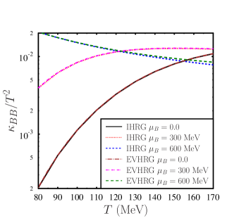
Figure 1: Variation of dimensionless ratio $\kappa_{BB}/T^{2}$ with temperature ($T$) and the baryon chemical potential ($\mu_{B}$). Here we have assumed $\mu_{Q}=0=\mu_{S}$. Physically $\kappa_{BB}$ is the measure of the baryon number current generation due to gradient in $\beta\mu_{B}$. Among all the hadrons baryonic contribution is dominant over mesonic contribution in $\kappa_{BB}/T^{2}$. Estimated values of $\kappa_{BB}/T^{2}$ are almost similar in IHRG and EVHRG models. Different curves are overlapping.

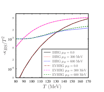
Figure 2: Variation of dimensionless ratio $-\kappa_{BS}/T^{2}$ with temperature ($T$) and the baryon chemical potential ($\mu_{B}$) for $\mu_{Q}=0=\mu_{S}$. For the range of thermodynamic parameters considered here $\kappa_{BS}$ is always negative. Physically $\kappa_{BS}$ is the measure of the diffusive coupling between the baryon number and the strangeness number. Among all the hadrons baryons contribute dominantly in $\kappa_{BS}/T^{2}$. Values of $\kappa_{BS}/T^{2}$ as obtained in IHRG and EVHRG models are very similar with overlapping curves.

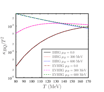
Figure 3: Variation of dimensionless ratio $\kappa_{BQ}/T^{2}$ with temperature ($T$) and the baryon chemical potential ($\mu_{B}$) for $\mu_{Q}=0=\mu_{S}$. $\kappa_{BQ}$ is the measure of the diffusive coupling between the baryon and electric charge. Among all the hadrons leading contribution in $\kappa_{BQ}/T^{2}$ comes from the baryons. Estimated values of $\kappa_{BQ}/T^{2}$ in IHRG and EVHRG models are very similar with overlapping curves.

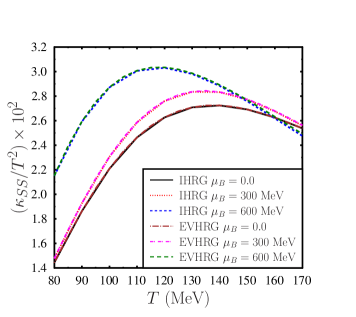
Figure 4: Variation of diagonal component $\kappa_{SS}/T^{2}$ with temperature ($T$) and the baryon chemical potential ($\mu_{B}$). Here also we consider the scenario with $\mu_{Q}=0=\mu_{S}$. $\kappa_{SS}$ is the measure of the strangeness number current due to the gradient in $\beta\mu_{S}$. Since the lightest strange hadrons are mesons, therefore mesonic contribution is dominant in $\kappa_{SS}/T^{2}$ with respect to the baryonic contribution. Estimated values of $\kappa_{SS}/T^{2}$ in IHRG and EVHRG models are very similar with overlapping curves.

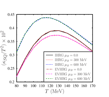
Figure 5: Variation of dimensionless ratio $\kappa_{SQ}/T^{2}$ with temperature ($T$) and the baryon chemical potential ($\mu_{B}$) for $\mu_{Q}=0=\mu_{S}$. $\kappa_{SQ}$ is the measure of the diffusive coupling between the strangeness charge and electric charge. Mesons contribute predominantly in $\kappa_{SQ}/T^{2}$. Different curves for IHRG and EVHRG are overlapping.

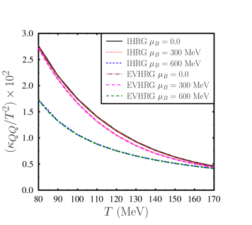
Figure 6: Variation of diagonal component $\kappa_{QQ}/T^{2}$ with temperature ($T$) and the baryon chemical potential ($\mu_{B}$). $\kappa_{QQ}$ is the measure of the electrical current due to the gradient in $\beta\mu_{Q}$. For the hadron resonance gas leading contribution to $\kappa_{QQ}/T^{2}$ comes from the mesons with respect to the hadrons. Similar to other elements of the diffusion matrix, $\kappa_{QQ}/T^{2}$ also has similar values in the IHRG and EVHRG model.

IV results and discussions

We present the results for the diffusion matrix elements $\kappa_{qq^{\prime}}$ with temperature and baryon chemical potential. For simplicity, we assume that electric chemical potential and the strangeness chemical potential is zero, i.e. $\mu_{Q}=0=\mu_{S}$. For HRG, we consider all the hadrons and their resonances up to a mass cutoff $\Lambda=2.6$ GeV, as is listed in Ref. ParticleDataGroup:2008zun . Also for a detailed list of hadrons and their resonances, we refer to Appendix A of Ref. PhysRevC.90.024915 . These apart radii of the hard spheres also enter in the calculation of relaxation time. We consider a uniform radius $R=0.5$ fm for all the hadrons PhysRevC.92.035203 ; Braun-Munzinger:1999hun .

In Fig. (1) we show the variation of the diagonal component of the diffusion matrix associated with the baryon number current, i.e. $\kappa_{BB}$ with temperature and baryon chemical potential. For $\mu_{B}=0$ and 300 MeV the dimensionless quantity $\kappa_{BB}/T^{2}$ increases with temperature. However for $\mu_{B}=600$ MeV, $\kappa_{BB}/T^{2}$ decreases with temperature. Since here we consider $\mu_{Q}=0=\mu_{S}$, for vanishing value of baryon chemical potential the variation of $\kappa_{BB}/T^{2}$ can be understood in the following manner. For $\mu_{B}=\mu_{Q}=\mu_{S}=0$, the net baryon number density vanishes, i.e. $n_{B}=0$. Note that with temperature the relaxation time of hadrons decreases. On the other hand with temperature the contribution coming from the distribution function increase due to the increase in the baryon numbers. This increase in the distribution function wins over the decrease in the relaxation time, giving rise to an increasing behavior of $\kappa_{BB}/T^{2}$ with temperature. However for $\mu_{B}\neq 0$, in the expression of $\kappa_{BB}$, $n_{B}/\omega$ increases with temperature Das:2019pqd along with the decreases in the relaxation time with temperature. For a sufficiently large value of the baryon chemical potential, this decrease in the relaxation time is predominant giving rise to a decreasing behavior of $\kappa_{BB}/T^{2}$ with temperature for $\mu_{B}=600$ MeV.

Further in the relatively low-temperature range $\kappa_{BB}/T^{2}$ increases with $\mu_{B}$. Note that for the hadron resonance gas with $\mu_{B}$, $n_{B}/\omega$ increases Das:2019pqd along with the increase in the distribution function. Again the relaxation time of various hadron species decreases with the baryon chemical potential. Such an increase in $n_{B}/\omega$ and distribution function dominates over the decreases in the relaxation time giving rise to an overall increasing trend. However, for a sufficiently high-temperature range, the variation of $\kappa_{BB}/T^{2}$ with the baryon chemical potential is nonmonotonic. This nonmonotonic variation is predominantly due to the decrease in the relaxation time with temperature and baryon chemical potential. Note that results for $\kappa_{BB}/T^{2}$ as obtained in the IHRG, as well as EVHRG, are almost similar. This is a generic feature for other components of the diffusion matrix. Various thermodynamic quantities, e.g. pressure, energy density, and number density are different in EVHRG as compared to the IHRG model. But the thermodynamic quantity that enters into the expression of $\kappa_{qq}$ is $n_{q}/\omega$. $n_{q}/\omega$ does not change significantly in the EVHRG as compared to the IHRG, giving rise to an almost similar variation of the diffusion matrix elements with temperature and baryon chemical potential.

In Fig. (2) we show the variation of $-\kappa_{BS}/T^{2}$ with temperature ($T$) and the baryon chemical potential ($\mu_{B}$). Physically a nonvanishing value of $\kappa_{BS}$ indicates the generation of baryon current due to the gradient in the number density of hadrons containing strangeness quantum number. Further note that $\kappa_{BS}$ is negative for the range of temperature and baryon chemical potential considered here. For $\mu_{B}=0$ this can be understood in the following way. For $\mu_{B}=\mu_{S}=\mu_{Q}=0$, $n_{B}=n_{S}=0$ and $\kappa_{BS}$ is proportional to the (baryon number $\times$ strangeness number). Now in the baryon sector, baryon number and strangeness number of various baryons are opposite in sign giving rise to a negative value of $\kappa_{BS}$. Also for finite $\mu_{B}$ baryon contributes dominantly in $\kappa_{BS}$ due to an increase in the number density of baryons. The opposite sign of the baryon number and the strangeness number for baryons give rise to an overall negative sign to $\kappa_{BS}$. Similar to $\kappa_{BB}/T^{2}$, the off-diagonal component $-\kappa_{BS}/T^{2}$ also shows strong temperature dependence for $\mu_{B}=0,300$ MeV. Such a behaviour is again predominantly due to increase in the equilibrium distribution function. The nonmonotonic variation of $-\kappa_{BS}/T^{2}$ with $\mu_{B}$ is again due to various $\mu_{B}$ dependent factors, e.g. relaxation time, $n_{B}/\omega$, $n_{S}/\omega$ and the equilibrium distribution function.

In Fig. (3) we show the variation $\kappa_{BQ}/T^{2}$ with temperature ($T$) and the baryon chemical potential ($\mu_{B}$). Similar to $\kappa_{BS}$ a nonvanishing value of $\kappa_{BQ}$ indicates gradient in the baryon number density can give rise to electric current. Further note that unlike $\kappa_{BS}$, $\kappa_{BQ}$ is positive for the range of temperature and baryon chemical potential considered here. Such behavior is easy to understand for $\mu_{B}=0$ case. As discussed earlier for $\mu_{B}=\mu_{S}=\mu_{Q}=0$, $n_{B}=n_{S}=0$ and $\kappa_{BQ}$ is proportional to the (baryon number $\times$ electric charge). Now in the baryon sector for the lightest baryon and antibaryons, baryon number and electric charge has the same sign giving rise to a positive value of $\kappa_{BQ}$. Similarly one can also explain the overall positive sign for $\kappa_{BQ}/T^{2}$at finite $\mu_{B}$. Variation of $\kappa_{BQ}/T^{2}$ with temperature and baryon chemical potential is very similar to $\kappa_{BB}/T^{2}$. Such variation of $\kappa_{BQ}/T^{2}$ with temperature and baryon chemical can be qualitatively understood by looking into the behavior of relaxation time, $n_{B}/\omega$, $n_{Q}/\omega$ and the equilibrium distribution function with $T$ and $\mu_{B}$.

In Figs. (4) and (5) we present the results for the diffusion coefficients associated with the strangeness current originated due to gradient in $\beta\mu_{S}$ and $\beta\mu_{Q}$ respectively. According to Eq. (45) the diagonal component $\kappa_{SS}/T^{2}$ is always positive. The off-diagonal component $\kappa_{SQ}/T^{2}$ is also positive for the range of temperature and baryon chemical potential considered here. Both $\kappa_{SS}/T^{2}$ and $\kappa_{SQ}/T^{2}$ shows nonmonotonic variation with temperature and baryon chemical potential. Such nonmontonic variation of $\kappa_{SS}/T^{2}$ and $\kappa_{SQ}/T^{2}$ is rather convoluted as various factors, e.g. the relaxation time, distribution function, $n_{S}/\omega$ and $n_{Q}/\omega$ depends upon temperature and baryon chemical potential. Although the behaviour of $\kappa_{BB}/T^{2}$, $\kappa_{BS}/T^{2}$ and $\kappa_{BQ}/T^{2}$ as presented in Figs. (1), (2) and (3) respectively, are similar to the results presented in the Refs. Fotakis:2019nbq ; Greif:2017byw , the nonmonotonic variation of $\kappa_{SS}/T^{2}$ and $\kappa_{SQ}/T^{2}$ is different from the results presented in the Refs. Fotakis:2019nbq ; Greif:2017byw .

Finally, in Fig. (6) we show the variation of $\kappa_{QQ}/T^{2}$ with $T$ and $\mu_{B}$. As argued in Refs. Fotakis:2019nbq ; Greif:2017byw , here also for $\mu_{B}=0$, $\kappa_{QQ}/T^{2}\equiv\sigma_{el}/T$. $\sigma_{el}$ is the electrical conductivity of the medium in the kinetic theory approach  Das:2019wjg . Although for non vanishing values of baryon chemical potential $\kappa_{QQ}/T^{2}\neq\sigma_{el}/T$, but the qualitative behaviour of $\kappa_{QQ}/T^{2}$ and $\sigma_{el}/T$ are similar even for $\mu_{B}\neq 0$ Das:2019wjg . Among all the other hadrons pions and protons contribute dominantly in $\sigma_{el}/T$ as well as in $\kappa_{QQ}/T^{2}$. As argued in Ref. Das:2019wjg among various temperature and baryon chemical potential dependent quantities, due to the decrease of the relaxation time of hadrons with $T$ and $\mu_{B}$, $\sigma_{el}/T$ or $\kappa_{QQ}/T^{2}$ also decreases.

V conclusion

In the present investigation, we discuss the diffusion matrix associated with the various conserved quantities. Using the classical kinetic theory within the relaxation time approximation we obtained an analytical expression of the diffusion matrix ($\kappa_{qq^{\prime}}$). The diagonal components of the diffusion matrix are always positive, on the other hand, the off-diagonal components can be negative as well as positive. Using the hadron resonance gas model within the hard-sphere scattering approximation we estimated various elements of $\kappa_{qq^{\prime}}$ for the hadronic medium produced in heavy-ion collisions. Knowledge of the diffusion processes and the diffusion currents is very important in the context of the bulk evolution of the strongly interacting plasma, e.g. the cross-coupling between the diffusion currents can dynamically generate non-zero net strangeness, even if it is initially zero Fotakis:2019nbq . Further, the order of magnitude values of the off-diagonal components of the diffusion matrix is not at all negligible as compared to the diagonal elements. Therefore, it is of paramount importance to computing the full table of diffusion coefficients for consistent fluid dynamical simulations where the diffusion is also taken under consideration. In this paper, we have ignored the effect of the mean-field or medium modification on the constituent of the plasma. Such mean-field effects should be included in the kinetic theory description as it might be quite important across the QCD transition scale.

Appendix A

Let us start with the following integration for a single species,

$$\mathcal{I}_{1} =\int\frac{d^{3}p}{(2\pi)^{3}}p^{2}\exp(-\beta\sqrt{p^{2}+m^{2}})$$

$$=\frac{m^{5}}{2\pi^{2}}\int_{0}^{\infty}dy~{}\cosh{y}~{}(\sinh{y})^{4}\exp(-\beta m\cosh{y})$$

$$=\frac{m^{5}}{2\pi^{2}}\int_{0}^{\infty}dy~{}((\cosh{y})^{5}-2(\cosh{y})^{3}+\cosh{y})$$

$$~{}~{}~{}~{}~{}~{}~{}~{}~{}~{}~{}~{}~{}~{}~{}~{}~{}~{}~{}~{}~{}~{}\times\exp(-\beta m\cosh{y})$$

$$=\frac{m^{5}}{2\pi^{2}}\bigg{(}\mathcal{I}_{1a}-2\mathcal{I}_{1b}+\mathcal{I}_{1c}\bigg{)},$$ (55)

here,

$$\mathcal{I}_{1a}=\int_{0}^{\infty}dy(\cosh{y})^{5}\exp(-\beta m\cosh{y}),$$ (56)

$$\mathcal{I}_{1b}=\int_{0}^{\infty}dy(\cosh{y})^{3}\exp(-\beta m\cosh{y}),$$ (57)

$$\mathcal{I}_{1c}=\int_{0}^{\infty}dy\cosh{y}\exp(-\beta m\cosh{y}).$$ (58)

Using the integral representation of the Modified Bessel Function of the second kind ($K_{n}(x)$) the integral it is easy to show that,

$$\mathcal{I}_{1c}=K_{1}(\beta m),$$ (59)

$$\mathcal{I}_{1b}=\frac{\partial^{2}K_{1}(\beta m)}{\partial(\beta m)^{2}}=\frac{1}{\beta m}K_{0}(\beta m)+\frac{2}{(\beta m)^{2}}K_{1}(\beta m)$$

$$~{}~{}~{}~{}~{}~{}~{}~{}~{}~{}~{}~{}~{}~{}~{}~{}~{}~{}~{}~{}~{}~{}~{}~{}~{}~{}~{}~{}~{}~{}~{}~{}~{}+K_{1}(\beta m)$$

$$~{}~{}~{}~{}~{}~{}~{}=\frac{1}{\beta m}K_{2}(\beta m)+K_{1}(\beta m),$$ (60)

$$\mathcal{I}_{1a}=\frac{\partial^{4}K_{1}(\beta m)}{\partial(\beta m)^{4}}$$

$$=\frac{12}{(\beta m)^{3}}K_{0}(\beta m)+\frac{2}{\beta m}K_{0}(\beta m)+\frac{24}{(\beta m)^{4}}K_{1}(\beta m)$$

$$~{}~{}~{}~{}~{}~{}~{}\frac{7}{(\beta m)^{2}}K_{1}(\beta m)+K_{1}(\beta m)$$

$$=\frac{3}{(\beta m)^{2}}K_{3}(\beta m)+\frac{2}{\beta m}K_{2}(\beta m)+K_{1}(\beta m).$$ (61)

Eqs. (59)-(61) allows us to write the integral $\mathcal{I}_{1}$ as,

$$\mathcal{I}_{1}=\frac{3m^{3}T^{2}}{2\pi^{2}}K_{3}(\beta m).$$ (62)

Now the energy density and pressure of a single particle species of mass $m$ at finite temperature $T$ can be expressed as Florkowski:2014sfa ,

$$\varepsilon=\frac{m^{2}T}{2\pi^{2}}\bigg{(}3TK_{2}(\beta m)+mK_{1}(\beta m)\bigg{)},$$ (63)

and,

$$P=\frac{m^{2}T^{2}}{2\pi^{2}}K_{2}(\beta m).$$ (64)

Therefore, the enthalpy ($\omega$) can be expressed as,

$$\omega =\varepsilon+P$$

$$=\frac{4m^{2}T^{2}}{2\pi^{2}}K_{2}(\beta m)+\frac{m^{3}T}{2\pi^{2}}K_{1}(\beta m)$$

$$=\frac{m^{3}T}{2\pi^{2}}K_{3}(\beta m)=\frac{1}{3T}\mathcal{I}_{1}.$$ (65)

The above expression can be generalized to multiple particle species.

Appendix B

We give here a short derivation of Eq.(40). Without loss of generality,let us consider only the baryon number conservation and a single baryon and it’s antibaryon species. In this case the integral,

$$\mathcal{I}_{2} =\sum_{a}q_{a}\int\frac{d^{3}p_{a}}{(2\pi)^{3}}\frac{p_{a}^{2}}{3E_{a}}\exp(-\beta\sqrt{p_{a}^{2}+m_{a}^{2}})\exp(\beta q_{a}\mu_{q})$$

$$=\int\frac{d^{3}p}{(2\pi^{3})}\frac{p^{2}}{3E}\exp(-\beta\sqrt{p^{2}+m^{2}})2\sinh(\beta\mu_{B})$$

$$=2\sinh(\beta\mu_{B})\frac{m^{4}}{6\pi^{2}}\int_{0}^{\infty}dy(\sinh{y})^{4}\exp(-\beta m\cosh{y})$$

$$=2\sinh(\beta\mu_{B})\frac{m^{4}}{6\pi^{2}}(\mathcal{I}_{2a}-2\mathcal{I}_{2b}+\mathcal{I}_{2c}),$$ (66)

here,

$$\mathcal{I}_{2a}=\int_{0}^{\infty}dy(\cosh{y})^{4}\exp(-\beta m\cosh{y}),$$ (67)

$$\mathcal{I}_{2b}=\int_{0}^{\infty}dy(\cosh{y})^{2}\exp(-\beta m\cosh{y}),$$ (68)

$$\mathcal{I}_{1c}=\int_{0}^{\infty}dy\exp(-\beta m\cosh{y}).$$ (69)

Using the integral representation of the Modified Bessel Function of the second kind ($K_{n}(x)$) it can be shown that,

$$\mathcal{I}_{2c}=K_{0}(\beta m),$$ (70)

$$\mathcal{I}_{2b}=K_{0}(\beta m)+\frac{1}{\beta m}K_{1}(\beta m),$$ (71)

$$\mathcal{I}_{2a}=\frac{3}{(\beta m)^{2}}K_{2}(\beta m)+K_{2}(\beta m).$$ (72)

Therefore,

$$\mathcal{I}_{2}=2\sinh(\beta\mu_{B})\frac{m^{2}T^{2}}{2\pi^{2}}K_{2}(\beta m).$$ (73)

Net baryon number density can be expressed as,

$$n_{B} =2\sinh{\beta\mu_{B}}\int\frac{d^{3}p}{(2\pi)^{3}}\exp(-\beta m\sqrt{p^{2}+m^{2}})$$

$$=2\sinh{\beta\mu_{B}}\frac{m^{2}T}{2\pi^{2}}K_{2}(\beta m).$$ (74)

Therefore,

$$\mathcal{I}_{2}=n_{B}T.$$ (75)

The above expression can be easily generalized to include other conserved charges.

References

- (1) P. Romatschke and U. Romatschke, Relativistic Fluid Dynamics In and Out of Equilibrium. Cambridge Monographs on Mathematical Physics. Cambridge University Press, 5, 2019. arXiv:1712.05815 [nucl-th].
- (2) W. Florkowski, Phenomenology of Ultra-Relativistic Heavy-Ion Collisions. 3, 2010.
- (3) C. Gale, S. Jeon, and B. Schenke, “Hydrodynamic Modeling of Heavy-Ion Collisions,” Int. J. Mod. Phys. A 28 (2013) 1340011, arXiv:1301.5893 [nucl-th].
- (4) S. Jeon and U. Heinz, “Introduction to Hydrodynamics,” Int. J. Mod. Phys. E 24 no. 10, (2015) 1530010, arXiv:1503.03931 [hep-ph].
- (5) A. Jaiswal and V. Roy, “Relativistic hydrodynamics in heavy-ion collisions: general aspects and recent developments,” Adv. High Energy Phys. 2016 (2016) 9623034, arXiv:1605.08694 [nucl-th].
- (6) U. Heinz and R. Snellings, “Collective flow and viscosity in relativistic heavy-ion collisions,” Ann. Rev. Nucl. Part. Sci. 63 (2013) 123–151, arXiv:1301.2826 [nucl-th].
- (7) P. Kovtun, D. T. Son, and A. O. Starinets, “Viscosity in strongly interacting quantum field theories from black hole physics,” Phys. Rev. Lett. 94 (2005) 111601, arXiv:hep-th/0405231.
- (8) S. Gavin, “TRANSPORT COEFFICIENTS IN ULTRARELATIVISTIC HEAVY ION COLLISIONS,” Nucl. Phys. A 435 (1985) 826–843.
- (9) A. Hosoya and K. Kajantie, “Transport Coefficients of QCD Matter,” Nucl. Phys. B 250 (1985) 666–688.
- (10) A. Dobado and J. M. Torres-Rincon, “Bulk viscosity and the phase transition of the linear sigma model,” Phys. Rev. D 86 (2012) 074021, arXiv:1206.1261 [hep-ph].
- (11) C. Sasaki and K. Redlich, “Bulk viscosity in quasi particle models,” Phys. Rev. C 79 (2009) 055207, arXiv:0806.4745 [hep-ph].
- (12) C. Sasaki and K. Redlich, “Transport coefficients near chiral phase transition,” Nucl. Phys. A 832 (2010) 62–75, arXiv:0811.4708 [hep-ph].
- (13) F. Karsch, D. Kharzeev, and K. Tuchin, “Universal properties of bulk viscosity near the QCD phase transition,” Phys. Lett. B 663 (2008) 217–221, arXiv:0711.0914 [hep-ph].
- (14) S. I. Finazzo, R. Rougemont, H. Marrochio, and J. Noronha, “Hydrodynamic transport coefficients for the non-conformal quark-gluon plasma from holography,” JHEP 02 (2015) 051, arXiv:1412.2968 [hep-ph].
- (15) A. Wiranata and M. Prakash, “Bulk Viscosity of Interacting Hadrons,” Nucl. Phys. A 830 (2009) 219C–222C, arXiv:0906.5592 [nucl-th].
- (16) S. Jeon and L. G. Yaffe, “From quantum field theory to hydrodynamics: Transport coefficients and effective kinetic theory,” Phys. Rev. D 53 (1996) 5799–5809, arXiv:hep-ph/9512263.
- (17) J. Noronha-Hostler, G. S. Denicol, J. Noronha, R. P. G. Andrade, and F. Grassi, “Bulk Viscosity Effects in Event-by-Event Relativistic Hydrodynamics,” Phys. Rev. C 88 no. 4, (2013) 044916, arXiv:1305.1981 [nucl-th].
- (18) S. Ryu, J. F. Paquet, C. Shen, G. S. Denicol, B. Schenke, S. Jeon, and C. Gale, “Importance of the Bulk Viscosity of QCD in Ultrarelativistic Heavy-Ion Collisions,” Phys. Rev. Lett. 115 no. 13, (2015) 132301, arXiv:1502.01675 [nucl-th].
- (19) S. Ryu, J.-F. Paquet, C. Shen, G. Denicol, B. Schenke, S. Jeon, and C. Gale, “Effects of bulk viscosity and hadronic rescattering in heavy ion collisions at energies available at the BNL Relativistic Heavy Ion Collider and at the CERN Large Hadron Collider,” Phys. Rev. C 97 no. 3, (2018) 034910, arXiv:1704.04216 [nucl-th].
- (20) G. Vujanovic, J.-F. Paquet, C. Shen, G. S. Denicol, S. Jeon, C. Gale, and U. Heinz, “Exploring the influence of bulk viscosity of QCD on dilepton tomography,” Phys. Rev. C 101 (2020) 044904, arXiv:1903.05078 [nucl-th].
- (21) K. Tuchin, “Photon decay in strong magnetic field in heavy-ion collisions,” Phys. Rev. C 83 (2011) 017901, arXiv:1008.1604 [nucl-th].
- (22) K. Tuchin, “Synchrotron radiation by fast fermions in heavy-ion collisions,” Phys. Rev. C 82 (2010) 034904, arXiv:1006.3051 [nucl-th]. [Erratum: Phys.Rev.C 83, 039903 (2011)].
- (23) G. Inghirami, L. Del Zanna, A. Beraudo, M. H. Moghaddam, F. Becattini, and M. Bleicher, “Numerical magneto-hydrodynamics for relativistic nuclear collisions,” Eur. Phys. J. C 76 no. 12, (2016) 659, arXiv:1609.03042 [hep-ph].
- (24) A. Das, S. S. Dave, P. S. Saumia, and A. M. Srivastava, “Effects of magnetic field on plasma evolution in relativistic heavy-ion collisions,” Phys. Rev. C 96 no. 3, (2017) 034902, arXiv:1703.08162 [hep-ph].
- (25) M. Greif, C. Greiner, and G. S. Denicol, “Electric conductivity of a hot hadron gas from a kinetic approach,” Phys. Rev. D 93 no. 9, (2016) 096012, arXiv:1602.05085 [nucl-th]. [Erratum: Phys.Rev.D 96, 059902 (2017)].
- (26) M. Greif, I. Bouras, C. Greiner, and Z. Xu, “Electric conductivity of the quark-gluon plasma investigated using a perturbative QCD based parton cascade,” Phys. Rev. D 90 no. 9, (2014) 094014, arXiv:1408.7049 [nucl-th].
- (27) A. Puglisi, S. Plumari, and V. Greco, “Shear viscosity to electric conductivity el ratio for the quark–gluon plasma,” Phys. Lett. B 751 (2015) 326–330, arXiv:1407.2559 [hep-ph].
- (28) A. Puglisi, S. Plumari, and V. Greco, “Electric Conductivity from the solution of the Relativistic Boltzmann Equation,” Phys. Rev. D 90 (2014) 114009, arXiv:1408.7043 [hep-ph].
- (29) W. Cassing, O. Linnyk, T. Steinert, and V. Ozvenchuk, “Electrical Conductivity of Hot QCD Matter,” Phys. Rev. Lett. 110 no. 18, (2013) 182301, arXiv:1302.0906 [hep-ph].
- (30) T. Steinert and W. Cassing, “Electric and magnetic response of hot QCD matter,” Phys. Rev. C 89 no. 3, (2014) 035203, arXiv:1312.3189 [hep-ph].
- (31) G. Aarts, C. Allton, A. Amato, P. Giudice, S. Hands, and J.-I. Skullerud, “Electrical conductivity and charge diffusion in thermal QCD from the lattice,” JHEP 02 (2015) 186, arXiv:1412.6411 [hep-lat].
- (32) G. Aarts, C. Allton, J. Foley, S. Hands, and S. Kim, “Spectral functions at small energies and the electrical conductivity in hot, quenched lattice QCD,” Phys. Rev. Lett. 99 (2007) 022002, arXiv:hep-lat/0703008.
- (33) A. Amato, G. Aarts, C. Allton, P. Giudice, S. Hands, and J.-I. Skullerud, “Electrical conductivity of the quark-gluon plasma across the deconfinement transition,” Phys. Rev. Lett. 111 no. 17, (2013) 172001, arXiv:1307.6763 [hep-lat].
- (34) S. Gupta, “The Electrical conductivity and soft photon emissivity of the QCD plasma,” Phys. Lett. B 597 (2004) 57–62, arXiv:hep-lat/0301006.
- (35) Y. Burnier and M. Laine, “Towards flavour diffusion coefficient and electrical conductivity without ultraviolet contamination,” Eur. Phys. J. C 72 (2012) 1902, arXiv:1201.1994 [hep-lat].
- (36) H. T. Ding, A. Francis, O. Kaczmarek, F. Karsch, E. Laermann, and W. Soeldner, “Thermal dilepton rate and electrical conductivity: An analysis of vector current correlation functions in quenched lattice QCD,” Phys. Rev. D 83 (2011) 034504, arXiv:1012.4963 [hep-lat].
- (37) O. Kaczmarek and M. Müller, “Temperature dependence of electrical conductivity and dilepton rates from hot quenched lattice QCD,” PoS LATTICE2013 (2014) 175, arXiv:1312.5609 [hep-lat].
- (38) R. Marty, E. Bratkovskaya, W. Cassing, J. Aichelin, and H. Berrehrah, “Transport coefficients from the Nambu-Jona-Lasinio model for ,” Phys. Rev. C 88 (2013) 045204, arXiv:1305.7180 [hep-ph].
- (39) Y. Aoki, G. Endrodi, Z. Fodor, S. D. Katz, and K. K. Szabo, “The Order of the quantum chromodynamics transition predicted by the standard model of particle physics,” Nature 443 (2006) 675–678, arXiv:hep-lat/0611014.
- (40) M. Asakawa and K. Yazaki, “Chiral Restoration at Finite Density and Temperature,” Nucl. Phys. A 504 (1989) 668–684.
- (41) S. Ejiri, “Canonical partition function and finite density phase transition in lattice QCD,” Phys. Rev. D 78 (2008) 074507, arXiv:0804.3227 [hep-lat].
- (42) M. A. Stephanov, K. Rajagopal, and E. V. Shuryak, “Event-by-event fluctuations in heavy ion collisions and the QCD critical point,” Phys. Rev. D 60 (1999) 114028, arXiv:hep-ph/9903292.
- (43) Y. Hatta and M. Stephanov, “Proton number fluctuation as a signal of the QCD critical endpoint,” Phys. Rev. Lett. 91 (2003) 102003, arXiv:hep-ph/0302002. [Erratum: Phys.Rev.Lett. 91, 129901 (2003)].
- (44) M. Asakawa, U. W. Heinz, and B. Muller, “Fluctuation probes of quark deconfinement,” Phys. Rev. Lett. 85 (2000) 2072–2075, arXiv:hep-ph/0003169.
- (45) S. Jeon and V. Koch, “Fluctuations of particle ratios and the abundance of hadronic resonances,” Phys. Rev. Lett. 83 (1999) 5435–5438, arXiv:nucl-th/9906074.
- (46) S. Ejiri, F. Karsch, and K. Redlich, “Hadronic fluctuations at the QCD phase transition,” Phys. Lett. B 633 (2006) 275–282, arXiv:hep-ph/0509051.
- (47) M. Kitazawa, M. Asakawa, and H. Ono, “Non-equilibrium time evolution of higher order cumulants of conserved charges and event-by-event analysis,” Phys. Lett. B 728 (2014) 386–392, arXiv:1307.2978 [nucl-th].
- (48) V. Skokov, B. Friman, and K. Redlich, “Volume Fluctuations and Higher Order Cumulants of the Net Baryon Number,” Phys. Rev. C 88 (2013) 034911, arXiv:1205.4756 [hep-ph].
- (49) S. Pal, G. Kadam, H. Mishra, and A. Bhattacharyya, “Effects of hadronic repulsive interactions on the fluctuations of conserved charges,” Phys. Rev. D 103 no. 5, (2021) 054015, arXiv:2010.10761 [hep-ph].
- (50) M. Asakawa and M. Kitazawa, “Fluctuations of conserved charges in relativistic heavy ion collisions: An introduction,” Prog. Part. Nucl. Phys. 90 (2016) 299–342, arXiv:1512.05038 [nucl-th].
- (51) S. Jeon and V. Koch, “Charged particle ratio fluctuation as a signal for QGP,” Phys. Rev. Lett. 85 (2000) 2076–2079, arXiv:hep-ph/0003168.
- (52) E. V. Shuryak and M. A. Stephanov, “When can long range charge fluctuations serve as a QGP signal?,” Phys. Rev. C 63 (2001) 064903, arXiv:hep-ph/0010100.
- (53) S. Pratt and C. Plumberg, “Determining the Diffusivity for Light Quarks from Experiment,” Phys. Rev. C 102 no. 4, (2020) 044909, arXiv:1904.11459 [nucl-th].
- (54) J. A. Fotakis, M. Greif, C. Greiner, G. S. Denicol, and H. Niemi, “Diffusion processes involving multiple conserved charges: A study from kinetic theory and implications to the fluid-dynamical modeling of heavy ion collisions,” Phys. Rev. D 101 no. 7, (2020) 076007, arXiv:1912.09103 [hep-ph].
- (55) A. Monnai, “Dissipative Hydrodynamic Effects on Baryon Stopping,” Phys. Rev. C 86 (2012) 014908, arXiv:1204.4713 [nucl-th].
- (56) STAR Collaboration, M. M. Aggarwal et al., “An Experimental Exploration of the QCD Phase Diagram: The Search for the Critical Point and the Onset of De-confinement,” arXiv:1007.2613 [nucl-ex].
- (57) STAR Collaboration, B. Mohanty, “STAR experiment results from the beam energy scan program at RHIC,” J. Phys. G 38 (2011) 124023, arXiv:1106.5902 [nucl-ex].
- (58) PHENIX Collaboration, J. T. Mitchell, “The RHIC Beam Energy Scan Program: Results from the PHENIX Experiment,” Nucl. Phys. A 904-905 (2013) 903c–906c, arXiv:1211.6139 [nucl-ex].
- (59) G. Odyniec, “The RHIC Beam Energy Scan program in STAR and what’s next …” J. Phys. Conf. Ser. 455 (2013) 012037.
- (60) STAR Collaboration, L. Adamczyk et al., “Bulk Properties of the Medium Produced in Relativistic Heavy-Ion Collisions from the Beam Energy Scan Program,” Phys. Rev. C 96 no. 4, (2017) 044904, arXiv:1701.07065 [nucl-ex].
- (61) B. Friman, C. Hohne, J. Knoll, S. Leupold, J. Randrup, R. Rapp, and P. Senger, eds., The CBM physics book: Compressed baryonic matter in laboratory experiments, vol. 814. 2011.
- (62) M. Greif, J. A. Fotakis, G. S. Denicol, and C. Greiner, “Diffusion of conserved charges in relativistic heavy ion collisions,” Phys. Rev. Lett. 120 no. 24, (2018) 242301, arXiv:1711.08680 [hep-ph].
- (63) P. Braun-Munzinger, K. Redlich, and J. Stachel, “Particle production in heavy ion collisions,” arXiv:nucl-th/0304013.
- (64) A. Andronic, P. Braun-Munzinger, and J. Stachel, “Hadron production in central nucleus-nucleus collisions at chemical freeze-out,” Nucl. Phys. A 772 (2006) 167–199, arXiv:nucl-th/0511071.
- (65) R. Dashen, S.-k. Ma, and H. J. Bernstein, “-matrix formulation of statistical mechanics,” Phys. Rev. 187 (Nov, 1969) 345–370.
- (66) R. F. Dashen and R. Rajaraman, “Narrow resonances in statistical mechanics,” Phys. Rev. D 10 (Jul, 1974) 694–708.
- (67) P. Braun-Munzinger, D. Magestro, K. Redlich, and J. Stachel, “Hadron production in Au - Au collisions at RHIC,” Phys. Lett. B 518 (2001) 41–46, arXiv:hep-ph/0105229.
- (68) J. Cleymans and K. Redlich, “Chemical and thermal freezeout parameters from 1-A/GeV to 200-A/GeV,” Phys. Rev. C 60 (1999) 054908, arXiv:nucl-th/9903063.
- (69) F. Becattini, J. Cleymans, A. Keranen, E. Suhonen, and K. Redlich, “Features of particle multiplicities and strangeness production in central heavy ion collisions between 1.7A-GeV/c and 158A-GeV/c,” Phys. Rev. C 64 (2001) 024901, arXiv:hep-ph/0002267.
- (70) J. Cleymans, B. Kampfer, M. Kaneta, S. Wheaton, and N. Xu, “Centrality dependence of thermal parameters deduced from hadron multiplicities in Au + Au collisions at s(NN)**(1/2) = 130-GeV,” Phys. Rev. C 71 (2005) 054901, arXiv:hep-ph/0409071.
- (71) A. Andronic, P. Braun-Munzinger, and J. Stachel, “Thermal hadron production in relativistic nuclear collisions: The Hadron mass spectrum, the horn, and the QCD phase transition,” Phys. Lett. B 673 (2009) 142–145, arXiv:0812.1186 [nucl-th]. [Erratum: Phys.Lett.B 678, 516 (2009)].
- (72) F. Karsch, K. Redlich, and A. Tawfik, “Thermodynamics at nonzero baryon number density: A Comparison of lattice and hadron resonance gas model calculations,” Phys. Lett. B 571 (2003) 67–74, arXiv:hep-ph/0306208.
- (73) P. Braun-Munzinger, V. Koch, T. Schäfer, and J. Stachel, “Properties of hot and dense matter from relativistic heavy ion collisions,” Phys. Rept. 621 (2016) 76–126, arXiv:1510.00442 [nucl-th].
- (74) M. Nahrgang, M. Bluhm, P. Alba, R. Bellwied, and C. Ratti, “Impact of resonance regeneration and decay on the net-proton fluctuations in a hadron resonance gas,” Eur. Phys. J. C 75 no. 12, (2015) 573, arXiv:1402.1238 [hep-ph].
- (75) A. Bhattacharyya, S. Das, S. K. Ghosh, R. Ray, and S. Samanta, “Fluctuations and correlations of conserved charges in an excluded volume hadron resonance gas model,” Phys. Rev. C 90 no. 3, (2014) 034909, arXiv:1310.2793 [hep-ph].
- (76) P. Garg, D. K. Mishra, P. K. Netrakanti, B. Mohanty, A. K. Mohanty, B. K. Singh, and N. Xu, “Conserved number fluctuations in a hadron resonance gas model,” Phys. Lett. B 726 (2013) 691–696, arXiv:1304.7133 [nucl-ex].
- (77) HotQCD Collaboration Collaboration, A. Bazavov, T. Bhattacharya, C. E. DeTar, H.-T. Ding, S. Gottlieb, R. Gupta, P. Hegde, U. M. Heller, F. Karsch, E. Laermann, L. Levkova, S. Mukherjee, P. Petreczky, C. Schmidt, R. A. Soltz, W. Soeldner, R. Sugar, and P. M. Vranas, “Fluctuations and correlations of net baryon number, electric charge, and strangeness: A comparison of lattice qcd results with the hadron resonance gas model,” Phys. Rev. D 86 (Aug, 2012) 034509.
- (78) V. V. Begun, M. I. Gorenstein, M. Hauer, V. P. Konchakovski, and O. S. Zozulya, “Multiplicity Fluctuations in Hadron-Resonance Gas,” Phys. Rev. C 74 (2006) 044903, arXiv:nucl-th/0606036.
- (79) M. Prakash, M. Prakash, R. Venugopalan, and G. Welke, “Nonequilibrium properties of hadronic mixtures,” Phys. Rept. 227 (1993) 321–366.
- (80) A. Wiranata and M. Prakash, “Shear Viscosities from the Chapman-Enskog and the Relaxation Time Approaches,” Phys. Rev. C 85 (2012) 054908, arXiv:1203.0281 [nucl-th].
- (81) P. Chakraborty and J. I. Kapusta, “Quasiparticle theory of shear and bulk viscosities of hadronic matter,” Phys. Rev. C 83 (Jan, 2011) 014906.
- (82) A. S. Khvorostukhin, V. D. Toneev, and D. N. Voskresensky, “Viscosity Coefficients for Hadron and Quark-Gluon Phases,” Nucl. Phys. A 845 (2010) 106–146, arXiv:1003.3531 [nucl-th].
- (83) S. Plumari, A. Puglisi, F. Scardina, and V. Greco, “Shear viscosity of a strongly interacting system: Green-kubo correlator versus chapman-enskog and relaxation-time approximations,” Phys. Rev. C 86 (Nov, 2012) 054902. https://link.aps.org/doi/10.1103/PhysRevC.86.054902.
- (84) M. I. Gorenstein, M. Hauer, and O. N. Moroz, “Viscosity in the excluded volume hadron gas model,” Phys. Rev. C 77 (Feb, 2008) 024911. https://link.aps.org/doi/10.1103/PhysRevC.77.024911.
- (85) J. Noronha-Hostler, J. Noronha, and C. Greiner, “Hadron mass spectrum and the shear viscosity to entropy density ratio of hot hadronic matter,” Phys. Rev. C 86 (Aug, 2012) 024913. https://link.aps.org/doi/10.1103/PhysRevC.86.024913.
- (86) S. K. Tiwari, P. K. Srivastava, and C. P. Singh, “Description of hot and dense hadron-gas properties in a new excluded-volume model,” Phys. Rev. C 85 (Jan, 2012) 014908. https://link.aps.org/doi/10.1103/PhysRevC.85.014908.
- (87) S. Ghosh, A. Lahiri, S. Majumder, R. Ray, and S. K. Ghosh, “Shear viscosity due to landau damping from the quark-pion interaction,” Phys. Rev. C 88 (Dec, 2013) 068201. https://link.aps.org/doi/10.1103/PhysRevC.88.068201.
- (88) S. Ghosh, G. a. Krein, and S. Sarkar, “Shear viscosity of a pion gas resulting from and interactions,” Phys. Rev. C 89 (Apr, 2014) 045201. https://link.aps.org/doi/10.1103/PhysRevC.89.045201.
- (89) A. Wiranata, V. Koch, M. Prakash, and X. N. Wang, “Shear viscosity of a multi-component hadronic system,” J. Phys. Conf. Ser. 509 (2014) 012049.
- (90) A. Wiranata, M. Prakash, and P. Chakraborty, “Comparison of Viscosities from the Chapman-Enskog and Relaxation Time Methods,” Central Eur. J. Phys. 10 (2012) 1349–1351, arXiv:1201.3104 [nucl-th].
- (91) A. Tawfik and M. Wahba, “Bulk and Shear Viscosity in Hagedorn Fluid,” Annalen Phys. 522 (2010) 849–856, arXiv:1005.3946 [hep-ph].
- (92) J. Noronha-Hostler, J. Noronha, and C. Greiner, “Transport coefficients of hadronic matter near ,” Phys. Rev. Lett. 103 (Oct, 2009) 172302. https://link.aps.org/doi/10.1103/PhysRevLett.103.172302.
- (93) G. P. Kadam and H. Mishra, “Bulk and shear viscosities of hot and dense hadron gas,” Nucl. Phys. A 934 (2014) 133–147, arXiv:1408.6329 [hep-ph].
- (94) G. Kadam, “Transport properties of hadronic matter in magnetic field,” Mod. Phys. Lett. A 30 no. 10, (2015) 1550031, arXiv:1412.5303 [hep-ph].
- (95) S. Ghosh, “A real-time thermal field theoretical analysis of Kubo-type shear viscosity: Numerical understanding with simple examples,” Int. J. Mod. Phys. A 29 (2014) 1450054, arXiv:1404.4788 [nucl-th].
- (96) N. Demir and A. Wiranata, “Hadronic Shear Viscosity: A Comparison between the Green-Kubo and Chapmann Enskog Methods,” J. Phys. Conf. Ser. 535 (2014) 012018.
- (97) S. Ghosh, “Nucleon thermal width owing to pion-baryon loops and its contributions to shear viscosity,” Phys. Rev. C 90 (Aug, 2014) 025202. https://link.aps.org/doi/10.1103/PhysRevC.90.025202.
- (98) J.-B. Rose, J. M. Torres-Rincon, A. Schäfer, D. R. Oliinychenko, and H. Petersen, “Shear viscosity of a hadron gas and influence of resonance lifetimes on relaxation time,” Phys. Rev. C 97 (May, 2018) 055204. https://link.aps.org/doi/10.1103/PhysRevC.97.055204.
- (99) C. Wesp, A. El, F. Reining, Z. Xu, I. Bouras, and C. Greiner, “Calculation of shear viscosity using green-kubo relations within a parton cascade,” Phys. Rev. C 84 (Nov, 2011) 054911. https://link.aps.org/doi/10.1103/PhysRevC.84.054911.
- (100) M. Greif, I. Bouras, C. Greiner, and Z. Xu, “Electric conductivity of the quark-gluon plasma investigated using a perturbative qcd based parton cascade,” Phys. Rev. D 90 (Nov, 2014) 094014. https://link.aps.org/doi/10.1103/PhysRevD.90.094014.
- (101) S. A. Bass et al., “Microscopic models for ultrarelativistic heavy ion collisions,” Prog. Part. Nucl. Phys. 41 (1998) 255–369, arXiv:nucl-th/9803035.
- (102) G. P. Kadam and H. Mishra, “Dissipative properties of hot and dense hadronic matter in an excluded-volume hadron resonance gas model,” Phys. Rev. C 92 (Sep, 2015) 035203. https://link.aps.org/doi/10.1103/PhysRevC.92.035203.
- (103) J. R. Bhatt, A. Das, and H. Mishra, “Thermoelectric effect and seebeck coefficient for hot and dense hadronic matter,” Phys. Rev. D 99 (Jan, 2019) 014015. https://link.aps.org/doi/10.1103/PhysRevD.99.014015.
- (104) A. Das and H. Mishra, “Thermoelectric transport coefficients of hot and dense QCD matter,” Eur. Phys. J. ST 230 no. 3, (2021) 607–634.
- (105) R. K. Mohapatra, H. Mishra, S. Dash, and B. K. Nandi, “Transport coefficients of hadronic matter in a van der Walls hadron resonance gas model,” arXiv:1901.07238 [hep-ph].
- (106) J. A. Fotakis, O. Soloveva, C. Greiner, O. Kaczmarek, and E. Bratkovskaya, “Diffusion coefficient matrix of the strongly interacting quark-gluon plasma,” arXiv:2102.08140 [hep-ph].
- (107) P. Chakraborty and J. I. Kapusta, “Quasi-Particle Theory of Shear and Bulk Viscosities of Hadronic Matter,” Phys. Rev. C 83 (2011) 014906, arXiv:1006.0257 [nucl-th].
- (108) M. Albright and J. I. Kapusta, “Quasiparticle Theory of Transport Coefficients for Hadronic Matter at Finite Temperature and Baryon Density,” Phys. Rev. C 93 no. 1, (2016) 014903, arXiv:1508.02696 [nucl-th].
- (109) M. Albright, Thermodynamics of Hot Hadronic Gases at Finite Baryon Densities. PhD thesis, Minnesota U., 2015.
- (110) P. Deb, G. P. Kadam, and H. Mishra, “Estimating transport coefficients in hot and dense quark matter,” Phys. Rev. D 94 no. 9, (2016) 094002, arXiv:1603.01952 [hep-ph].
- (111) J.-Y. Ollitrault, “Relativistic hydrodynamics for heavy-ion collisions,” Eur. J. Phys. 29 (2008) 275–302, arXiv:0708.2433 [nucl-th].
- (112) L. Onsager, “Reciprocal relations in irreversible processes. i.” Phys. Rev. 37 (Feb, 1931) 405–426.
- (113) L. Onsager, “Reciprocal relations in irreversible processes. ii.” Phys. Rev. 38 (Dec, 1931) 2265–2279.
- (114) P. L. Bhatnagar, E. P. Gross, and M. Krook, “A model for collision processes in gases. i. small amplitude processes in charged and neutral one-component systems,” Phys. Rev. 94 (May, 1954) 511–525. https://link.aps.org/doi/10.1103/PhysRev.94.511.
- (115) G. S. Rocha, G. S. Denicol, and J. Noronha, “Novel Relaxation Time Approximation to the Relativistic Boltzmann Equation,” arXiv:2103.07489 [nucl-th].
- (116) V. V. Begun, M. Gaździcki, and M. I. Gorenstein, “Hadron-resonance gas at freeze-out: Reminder on the importance of repulsive interactions,” Phys. Rev. C 88 (Aug, 2013) 024902.
- (117) A. Andronic, P. Braun-Munzinger, J. Stachel, and M. Winn, “Interacting hadron resonance gas meets lattice QCD,” Phys. Lett. B 718 (2012) 80–85, arXiv:1201.0693 [nucl-th].
- (118) D. H. Rischke, M. I. Gorenstein, H. Stoecker, and W. Greiner, “Excluded volume effect for the nuclear matter equation of state,” Z. Phys. C 51 (1991) 485–490.
- (119) Y. Hama, T. Kodama, and O. Socolowski, Jr., “Topics on hydrodynamic model of nucleus-nucleus collisions,” Braz. J. Phys. 35 (2005) 24–51, arXiv:hep-ph/0407264.
- (120) K. Werner, I. Karpenko, T. Pierog, M. Bleicher, and K. Mikhailov, “Event-by-event simulation of the three-dimensional hydrodynamic evolution from flux tube initial conditions in ultrarelativistic heavy ion collisions,” Phys. Rev. C 82 (Oct, 2010) 044904. https://link.aps.org/doi/10.1103/PhysRevC.82.044904.
- (121) G. P. Kadam and H. Mishra, “Dissipative properties of hot and dense hadronic matter in an excluded-volume hadron resonance gas model,” Phys. Rev. C 92 no. 3, (2015) 035203, arXiv:1506.04613 [hep-ph].
- (122) P. Braun-Munzinger, J. Stachel, J. P. Wessels, and N. Xu, “Thermal equilibration and expansion in nucleus-nucleus collisions at the AGS,” Phys. Lett. B 344 (1995) 43–48, arXiv:nucl-th/9410026.
- (123) R. Hagedorn and J. Rafelski, “Hot Hadronic Matter and Nuclear Collisions,” Phys. Lett. B 97 (1980) 136.
- (124) J. Cleymans, M. I. Gorenstein, J. Stalnacke, and E. Suhonen, “Excluded volume effect and the quark - hadron phase transition,” Phys. Scripta 48 (1993) 277–280.
- (125) G. D. Yen, M. I. Gorenstein, W. Greiner, and S. N. Yang, “Excluded volume hadron gas model for particle number ratios in collisions,” Phys. Rev. C 56 (Oct, 1997) 2210–2218. https://link.aps.org/doi/10.1103/PhysRevC.56.2210.
- (126) Particle Data Group Collaboration, C. Amsler et al., “Review of Particle Physics,” Phys. Lett. B 667 (2008) 1–1340.
- (127) M. Albright, J. Kapusta, and C. Young, “Matching excluded-volume hadron-resonance gas models and perturbative qcd to lattice calculations,” Phys. Rev. C 90 (Aug, 2014) 024915.
- (128) P. Braun-Munzinger, I. Heppe, and J. Stachel, “Chemical equilibration in Pb + Pb collisions at the SPS,” Phys. Lett. B 465 (1999) 15–20, arXiv:nucl-th/9903010.
- (129) A. Das, H. Mishra, and R. K. Mohapatra, “Transport coefficients of hot and dense hadron gas in a magnetic field: a relaxation time approach,” Phys. Rev. D 100 no. 11, (2019) 114004, arXiv:1909.06202 [hep-ph].
- (130) A. Das, H. Mishra, and R. K. Mohapatra, “Electrical conductivity and Hall conductivity of a hot and dense hadron gas in a magnetic field: A relaxation time approach,” Phys. Rev. D 99 no. 9, (2019) 094031, arXiv:1903.03938 [hep-ph].
- (131) W. Florkowski, E. Maksymiuk, R. Ryblewski, and M. Strickland, “Exact solution of the (0+1)-dimensional Boltzmann equation for a massive gas,” Phys. Rev. C 89 no. 5, (2014) 054908, arXiv:1402.7348 [hep-ph].