UnDeepLIO: Unsupervised Deep Lidar-Inertial Odometry

Abstract

Extensive research efforts have been dedicated to deep learning based odometry. Nonetheless, few efforts are made on the unsupervised deep lidar odometry. In this paper, we design a novel framework for unsupervised lidar odometry with the IMU, which is never used in other deep methods. First, a pair of siamese LSTMs are used to obtain the initial pose from the linear acceleration and angular velocity of IMU. With the initial pose, we perform the rigid transform on the current frame and align it to the last frame. Then we extract vertex and normal features from the transformed point clouds and its normals. Next a two-branch attention module is proposed to estimate residual rotation and translation from the extracted vertex and normal features, respectively. Finally, our model outputs the sum of initial and residual poses as the final pose. For unsupervised training, we introduce an unsupervised loss function which is employed on the voxelized point clouds. The proposed approach is evaluated on the KITTI odometry estimation benchmark and achieves comparable performances against other state-of-the-art methods.

1 Introduction

The task of odometry is to estimate 3D translation and orientation of autonomous vehicles which is one of key steps in SLAM. Autonomous vehicles usually collect information by perceiving the surrounding environment in real time and use on-board sensors such as lidar, Inertial Measurement Units (IMU), or camera to estimate their 3D translation and orientation. Lidar can provide high-precision 3D measurements but also has no requirement for light. The point clouds generated by the lidar can provide high-precision 3D measurements, but if it has large translation or orientation in a short time, the continuously generated point clouds will only get few matching points, which will affect the accuracy of odometry. IMU has advantages of high output frequency and directly outputting the 6DOF information to predict the initial translation and orientation that the localization failure phenomenon can be reduced when lidar has large translation or orientation.
The traditional methods [1, 19, 24, 20] are mainly based on the point registration and work well in ideal environments. However, due to the sparseness and irregularity of the point clouds, these methods are difficult to obtain enough matching points. Typically, ICP [1] and its variants [19, 14] iteratively find matching points which depend on nearest-neighbor searching and optimize the translation and orientation by matching points. This optimization procedure is sensitive to noise and dynamic objects and prone to getting stuck into the local minima.
Thanks to the recent advances in deep learning, many approaches adopt deep neural networks for lidar odometry, which can achieve more promising performance compared to traditional methods. But most of them are supervised methods [12, 25, 22, 13, 21, 10]. However, supervised methods require ground truth pose, which consumes a lot of manpower and material resources. Due to the scarcity of the ground truth, recent unsupervised methods are proposed [5, 15, 23], but some of them obtain unsatisfactory performance, and some need to consume a lot of video memory and time to train the network.
Two issues exist in these methods. First, these methods ignore IMU, which often bring fruitful clues for accurate lidar odometry. Second, those methods do not make full use of the normals, which only take the point clouds as the inputs. Normals of point clouds can indicate the relationship between a point and its surrounding points. And even if those approaches [12] who use normals as network input, they simply concatenate points and normals together and put them into network, but only orientation between two point clouds relates to normals, so normals should not be used to estimate translation.
To circumvent the dependence on expensive ground truth, we propose a novel framework termed as UnDeepLIO, which makes full use of the IMU and normals for more accurate odometry. We compare against various baselines using point clouds from the KITTI Vision Benchmark Suite [7] which collects point clouds using a $360^{\circ}$ Velodyne laser scanner.
Our main contributions are as follows:
$\bullet$ We present a self-supervised learning-based approach for robot pose estimation. our method can outperform [5, 15].
$\bullet$ We use IMU to assist odometry. Our IMU feature extraction module can be embedded in most network structures [12, 22, 5, 15].
$\bullet$ Both points and its normals are used as network inputs. We use feature of points to estimate translation and feature of both of them to estimate orientation.

2 Related Work

2.1 Model-based Odometry Estimation

Gauss-Newton iteration methods have a long-standing history in odometry task. Model-based methods solve odometry problems generally by using Newton’s iteration method to adjust the transformation between frames so that the ”gap” between frames keeps getting smaller. They can be categorized into two-frame methods [1, 19, 14] and multi-frame methods [24, 20].
Point registration is the most common skill for two-frame methods, where ICP [1] and its variants [19, 14] are typical examples. The ICP iteratively search key points and its correspondences to estimate the transformation between two point clouds until convergence. Moreover, most of these methods need multiple iterations with a large amount of calculation, which is difficult to meet the real-time requirements of the system.
Multi-frame algorithms [24, 20, 2] often relies on the two-frame based estimation. They improve the steps of selecting key points and finding matching points, and use additional mapping step to further optimize the pose estimation. Their calculation process is generally more complicated and runs at a lower frequency.

2.2 Learning-based Odometry Estimation

In the last few years, the development of deep learning has greatly affected the most advanced odometry estimation. Learning-based model can provide a solution only needs uniformly down sampling the point clouds without manually selecting key points. They can be classified into supervised methods and unsupervised methods.
Supervised methods appear relatively early, Lo-net [12] maps the point clouds to 2D ”image” by spherical projection. Wang et al. [22] adopt a dual-branch architecture to infer 3-D translation and orientation separately instead of a single network. Velas et al. [21] use point clouds to assist 3D motion estimation and regarded it as a classification problem. Differently, Li et al. [13] do not simply estimate 3D motion with fully connected layer but Singular Value Decomposition (SVD). Use Pointnet [18] as base net, Zheng et al. [25] propose a new approach for extracting matching keypoint pairs(MKPs) of consecutive LiDAR scans by projecting 3D point clouds into 2D spherical depth images where MKPs can be extracted effectively and efficiently.
Unsupervised methods appear later. Cho et al. [5] first apply unsupervised approach on deep-learning-based LiDAR odometry which is an extension of their previous approach [4]. The inspiration of its loss function comes from point-to-plane ICP [14]. Then, Nubert et al. [15] report methods with similarly models and loss function, but they use different way to calculate normals of each point in point clouds and find matching points between two continuous point clouds.

3 Methods

3.1 Data Preprocess

3.1.1 Data input

At every timestamp $k\in\mathbb{R}^{+}$, we can obtain one point clouds $P_{k}$ of $N*3$ dimensions and between every two timestamps we can get $S$ frames IMU $I_{k,k+1}$ of $S*6$ dimensions including 3D angular velocity and 3D linear acceleration . we take above data as the inputs.

3.1.2 Vertex map

In order to circumvent the disordered nature of point clouds, we project the point clouds into the 2D image coordinate system according to the horizontal and vertical angle. We employ projection function $\Pi:{\mathbb{R}}^{3}\mapsto{\mathbb{R}}^{2}$. Each 3D point $\bm{p}=(p_{x},p_{y},p_{z})$ in a point clouds $P_{k}$ is mapped into the 2D image plane $(w,h)$ represented as

$$\begin{split}\left(\begin{array}[]{c}w\\ h\\ \end{array}\right)=&\left(\begin{array}[]{c}(f_{w}-\arctan(\frac{p_{y}}{p_{x}}))/\eta_{w}\\ (f_{h}-\arcsin(\frac{p_{z}}{d}))/\eta_{h}\\ \end{array}\right),\\ &H>h\geq 0,W>w\geq 0,\end{split}$$ (1)

where depth is $d=\sqrt{{p_{x}}^{2}+{p_{y}}^{2}+{p_{z}}^{2}}$. $f_{w}$ and $f_{h}$ are the maximum horizontal and vertical angle. $H$ and $W$ are shape of vertex map. $f_{h}$ depends on the type of the lidar. $\eta_{w}$ and $\eta_{h}$ control the horizontal and vertical sampling density. If several 3D points correspond the same pixel values, we choose the point with minimum depth as the final result. If one pixel coordinate has no matching 3D points, the pixel value is set to $(0,0,0)$. We define the 2D image plane as vertex map $\bm{V}$.

3.1.3 Normal map

The normal vector of one point includes its relevance about the surrounding points, so we compute a normal map $\bm{N}$ which consists of normals $\bm{n}$ and has the same shape as corresponding vertex map $\bm{V}$. We adopt similar operations with Cho et al. [5] and Li et al. [12] to calculate the normal vectors. Each normal vector $\bm{n}$ corresponds to a vertex $\bm{v}$ with the same image coordinate. Due to sparse and discontinuous characteristics of point clouds, we pay more attention on the vertex with small Euclidean distance from the surrounding pixel via a pre-defined weight, which can be expressed as $w_{a,b}=e^{\{-0.5|d(v_{a})-d(v_{b})|\}}$. Each normal vector $\bm{n}$ is represented as

$$\bm{n}_{p}=\sum_{i\in[0,3]}w_{p_{i},p}(v_{p_{i}}-v_{p})\times w_{p_{i+1},p}(v_{p_{i+1}}-v_{p}),$$ (2)

where $p_{i}$ represents points in 4 directions of the central vertex $p$ (0-up, 1-right, 2-down, 3-left).

3.2 Network Structure

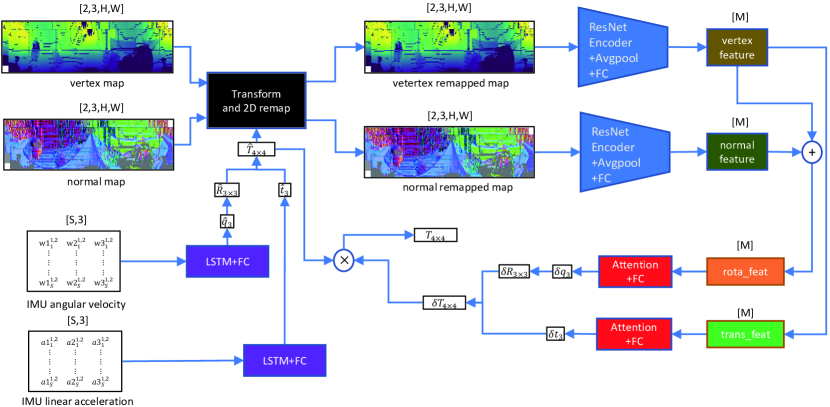
Figure 1: The proposed network and our unsupervised training scheme. FC represents fully connected layer. $t$ means translation and $q$ means Euler angle of orientation. LSTM takes continuous frames of IMU as inputs and output initial relative pose $\hat{T}$. $\hat{T}$ are used to transform two maps of current frame to last frame. Then we send the remapped maps into ResNet Encoder, which outputs feature maps, including vertex and normal features. From the features, we propose an attention layer to estimate residual pose $\delta T$. The final output is their sum $T=\delta T\hat{T}$.

3.2.1 Network input

Our pipeline is shown in the Fig. 1. Each point clouds associates with a vertex/normal map of $(3,H,W)$ dimensions, so we concatenate the vertex/normal map of $k$ and $k+1$ timestamp to get vertex/normal pair of $(2,3,H,W)$ dimensions. We take a pair of vertex/normal maps and IMU between $k$ and $k+1$ timestamp as the inputs of our model, where the IMU consists of the linear acceleration and angular velocity both of $(S,3)$ dimensions, and $S$ is the length of IMU sequence. Our model outputs relative pose $T_{k,k+1}$, where $R_{k,k+1}$ is orientation and $t_{k,k+1}$ is translation.

$$T_{k,k+1}^{4\times 4}=\left[\begin{array}[]{cc}R_{k,k+1}^{3\times 3}&t_{k,k+1}^{3\times 1}\\ 0&1\end{array}\right],$$ (3)

3.2.2 Estimating initial relative pose from IMU

Linear acceleration is used to estimate translation and angular velocity is used to estimate orientation. We employ LSTM on IMU to extract the features of IMU. Then the features are forwarded into the FC layer to estimate initial relative translation or orientation.

3.2.3 Mapping the point clouds of current frame to the last frame

Each vertex/normal pair consists of last and current frames. They are not in the same coordinate due to the transformation. The initial relative pose can map current frame in current coordinate to last coordinate, then we can obtain the remapped current map with the same size as the old one. The relationship between two maps are shown as formula (4). Take the $\bm{v}_{k+1,p}^{k}$ for example, it is the mapped vertex at timestamp $k$ from timestamp $k+1$ via the initial pose.

$$\bm{v}_{k+1,p}^{k}=R_{k,k+1}\bm{v}_{k+1,p}^{k+1}+t_{k,k+1},$$ (4)

$$\bm{n}_{k+1,p}^{k}=R_{k,k+1}\bm{n}_{k+1,p}^{k+1}.$$ (5)

3.2.4 Estimating residual relative pose from the remapped maps

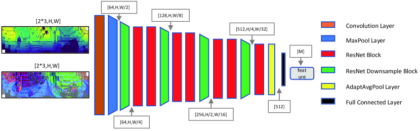
Figure 2: The detail structure of ResNet Encoder + Avgpool + FC part.

We use ResNet Encoder (see Fig. 2) as our map feature extractor. ResNet [8] is used in image recognition. Its input is the 2D images similar to us. Therefore, this structure can extract feature in our task as well. we send the remapping vertex/normal map pair into siamese ResNet Encoder, which outputs feature maps, including vertex and normal features. From the features, we propose an attention layer (by formula (6), $x$ is input) which is inspired by LSTM [9] to estimate residual pose $\delta T$ between last frame and the remapped current frame. . Among them, vertex and normal features are combined to estimate orientation, but only vertex is used to estimate translation because the change of translation does not cause the change of normal vectors. Together with initial relative pose, we can get final relative pose $T$.

$$\begin{split}&i=\sigma(W_{i}x+b_{i}),\\ &g=tanh(W_{g}x+b_{g}),\\ &o=\sigma(W_{o}x+b_{o}),\\ &out=o*tanh(i*g).\end{split}$$ (6)

3.3 Loss Function

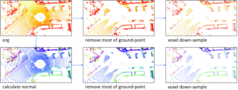
Figure 3: Point downsample process, including point (up) and normal (down).

For unsupervised training, we use a combination of geometric losses in our deep learning framework. Unlike Cho et al. [5] who use pixel locations as correspondence between two point clouds, we search correspondence on the whole point clouds. For speeding up calculation, we first calculate the normals $NP_{i}$ of whole point clouds $P_{i}$ by plane fitting $\Phi$ [17], and then remove its ground points by RANSAC [6], at last perform voxel grid filtering $\Downarrow$ (the arithmetic average of all points in voxel as its representation. The normal vectors of voxel are processed in the same way and standardized after downsample.) to downsample to about $K$ points (The precess is shown in Fig. 3). Given the predicted relative pose $T_{k,k+1}$, we apply it on preprocessed current point clouds $DP_{k+1}$ and its normals $NP_{k+1}$. For the correspondence search, we use KD-Tree [3] to find the nearest point in the last point clouds $DP_{k}$ of each point in the transformed current point clouds $\overline{DP}_{k+1}$.

$$\begin{split}&DP_{i}=\Downarrow(\mathsf{RANSAC}(P_{i})),\\ &NP_{i}=\Downarrow(\mathsf{RANSAC}(\Phi(P_{i})),\end{split}$$ (7)

$$\begin{split}&\overline{NP}_{k+1}=R_{k,k+1}NP_{k+1},\\ &\overline{DP}_{k+1}=R_{k,k+1}DP_{k+1}+t_{k,k+1}.\end{split}$$ (8)

3.3.1 Point-to-plane ICP loss

We use every point $\overline{dp}_{k+1}$ in current point clouds $\overline{DP}_{k+1}$, corresponding point of ${dp}_{k}$ and normal vector of ${np}_{k}$ in last point clouds ${DP}_{k}$ to compute the distance between point and its matching plane. The loss function $\mathcal{L}_{po2pl}$ is represented as

$$\mathcal{L}_{po2pl}=\sum_{\overline{dp}_{k+1}\in\overline{DP}_{k+1}}|{np}_{k}\centerdot(\overline{dp}_{k+1}-{dp}_{k})|_{1},$$ (9)

where $\centerdot$ denotes element-wise product.

3.3.2 Plane-to-plane ICP loss

Similarly to point-to-plane ICP, we use normal $\overline{np}_{k+1}$ of every point in $\overline{NP}_{k+1}$, corresponding normal vector of ${np}_{k}$ in ${NP}_{k}$ to compute the angle between a pair of matching plane. The loss function $\mathcal{L}_{pl2pl}$ is represented as

$$\mathcal{L}_{pl2pl}=\sum_{\overline{np}_{k+1}\in\overline{NP}_{k+1}}|\overline{np}_{k+1}-{np}_{k}|^{2}_{2}.$$ (10)

3.3.3 Overall loss

Finally, the overall unsupervised loss is obtained as

$$\mathcal{L}=\alpha\mathcal{L}_{po2pl}+\lambda\mathcal{L}_{po2pl},$$ (11)

where $\alpha$ and $\lambda$ are balancing factors.

4 Experiments

In this section, we first introduce implementation details of our model and benchmark dataset used in our experiments and the implementation details of the proposed model. Then, comparing to the existing lidar odometry methods, our model can obtain competitive results. Finally, we conduct ablation studies to verify the effectiveness of the innovative part of our model.

4.1 Implementation Details

The proposed network is implemented in PyTorch [16] and trained with a single NVIDIA Titan RTX GPU. We optimize the parameters with the Adam optimizer [11] whose hyperparameter values are $\beta_{1}=0.9$, $\beta_{2}=0.99$ and $w_{decay}=10^{-5}$. We adopt step scheduler with a step size of 20 and $\gamma=0.5$ to control the training procedure, the initial learning rate is $10^{-4}$ and the batch size is 20. The length $S$ of IMU sequence is 15. The maximum horizontal and vertical angle of vertex map are $f_{w}=180^{\circ}$ and $f_{h}=23^{\circ}$, and density of them are $\eta_{w}=\eta_{h}=0.5$. The shapes of input maps are $H=52$ and $W=720$. The loss weight of formula (11) is set to be $\alpha=1.0$ and $\lambda=0.1$. The initial side length of voxel downsample is set to 0.3m, it is adjusted according to the number of points after downsample, if points are too many, we increase the side length, otherwise reduce. The adjustment size is 0.01m per time. The number of points after downsample is controlled within $K\pm 100$ and $K=10240$.

4.2 Datasets

The KITTI odometry dataset [7] has 22 different sequences with images, 3D lidar point clouds, IMU and other data. Only sequences 00-10 have an official public ground truth. Among them, only sequence 03 does not provide IMU. Therefore, we do not use sequence 03 when there exists the IMU assist in our method.

4.3 Evaluation on the KITTI Dataset

We compare our method with the following methods which can be divided into two types. Model-based methods are: LOAM [24] and LeGO-LOAM [20]. Learning-based methods are: Nubert et al. [15], Cho et al. [5] and SelfVoxeLO [23].
In model-based methods, we show the lidar odometry results of them with mapping and without mapping.
In learning-based methods, we use two ways to divide the train and test set. First, we use sequences 00-08 for training and 09-10 for testing, as Cho et al. [5] and Nubert et al. [15] use Sequences 00-08 as their training set. We name it as ”Ours-easy”. Then, we use sequences 00-06 for training and 07-10 for testing, to compare with SelfVoxeLO which uses Sequences 00-06 as training set. We name it as ”Ours-hard”.
Table. 1 contains the details of the results: $t_{rel}$ means average translational RMSE (%) on length of 100m-800m and $r_{rel}$ means average rotational RMSE (^∘/100m) on length of 100m-800m. LeGO-LOAM is not always more precise by adding imu, traditional method is more sensitive to the accuracy of imu (In sequence 00, there exists some lack of IMU), which is most likely the reason for its accuracy drop. Even if the accuracy of the estimation is improved by the IMU, the effect is not obvious, especially after the mapping step. Our method gains a significant improvement by using IMU in test set, and has a certain advantage over traditional method without mapping, and is not much lower than with mapping. In the easy task (For trajectories results, see Fig. 4), our method without imu assist is also competitive compared to Cho et al. [5] and Nubert et al. [15] which also project the point clouds into the 2D image coordinate system. Our method can acquire a lot of improvements with imu. In the hard task, comparing to the most advanced method SelfVoxeLO [23] which uses 3D convolutions on voxels and consumes much video memory and training time, our method also can get comparable results with IMU. Since they did not publish the code, we are unable to conduct experiments on their method with imu.

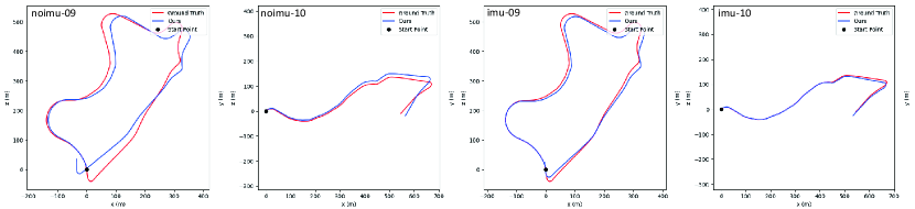
Figure 4: 2D estimated trajectories of our method on sequence 09 and 10.

Table 1: KITTI odometry evaluation.

$t_{rel}(\%)$	00	01	02	03	04	05	06	07	08	09	10	trainavg	testavg
LeGO-LOAM(w/ map)[20]	1.44	21.12	2.69	1.73	1.70	0.98	0.87	0.77	1.35	1.46	1.84	3.27
LeGO-LOAM(w/ map)+imu	7.24	20.07	2.56	x	1.68	0.82	0.86	0.67	1.29	1.49	1.75	3.84
LeGO-LOAM(w/o map)	6.98	26.52	6.92	6.16	3.64	4.57	5.16	4.05	6.01	5.22	7.73	7.54
LeGO-LOAM(w/o map)+imu	10.46	22.38	6.05	x	2.04	1.98	2.98	2.99	3.23	3.29	2.74	5.81
LOAM(w/ map)[24]	1.10	2.79	1.54	1.13	1.45	0.75	0.72	0.69	1.18	1.20	1.51	1.28
LOAM(w/o map)	15.99	3.43	9.40	18.18	9.59	9.16	8.91	10.87	12.72	8.10	12.67	10.82
Nubert et al.[15]	NA	NA	NA	NA	NA	NA	NA	NA	NA	6.05	6.44	3.00	6.25
Cho et al.[5]	NA	NA	NA	NA	NA	NA	NA	NA	NA	4.87	5.02	3.68	4.95
Ours-easy	1.33	3.40	1.53	1.43	1.26	1.22	1.19	0.97	1.92	3.87	2.69	1.58	3.28
Ours-easy+imu	1.50	3.44	1.33	x	0.94	0.98	0.90	1.00	1.63	2.24	1.83	1.46	2.03
SelfVoxelLO[23]	NA	NA	NA	NA	NA	NA	NA	3.09	3.16	3.01	3.48	2.50	3.19
Ours-hard	1.58	3.42	2.27	2.53	0.96	1.36	0.99	6.58	6.89	5.77	4.04	1.87	5.82
Ours-hard+imu	1.38	3.46	1.42	x	0.98	1.26	0.94	3.45	4.05	2.77	2.16	1.57	3.11
$r_{rel}(^{\circ}/100m)$	00	01	02	03	04	05	06	07	08	09	10	trainavg	testavg
LeGO-LOAM(w/ map)	0.65	2.17	0.99	0.99	0.69	0.47	0.45	0.51	0.58	0.64	0.74	0.81
LeGO-LOAM(w/ map)+imu	2.44	0.61	0.91	x	0.59	0.38	0.43	0.38	0.53	0.58	0.63	0.75
LeGO-LOAM(w/o map)	3.27	4.61	3.10	3.42	2.98	2.38	2.24	2.41	2.85	2.61	4.03	3.08
LeGO-LOAM(w/o map)+imu	3.72	1.79	2.12	x	0.88	0.88	1.24	1.64	1.23	1.75	1.57	1.68
LOAM(w/ map)	0.53	0.55	0.55	0.65	0.50	0.38	0.39	0.50	0.44	0.48	0.57	0.50
LOAM(w/o map)	6.25	0.93	3.68	9.91	4.57	4.10	4.63	6.76	5.77	4.30	8.79	5.43
Nubert et al.	NA	NA	NA	NA	NA	NA	NA	NA	NA	2.15	3.00	1.38	2.58
Cho et al.	NA	NA	NA	NA	NA	NA	NA	NA	NA	1.95	1.83	0.87	1.89
Ours-easy	0.69	0.97	0.68	1.04	0.73	0.66	0.64	0.58	0.78	1.67	1.97	0.75	1.82
Ours-easy+imu	0.70	0.99	0.59	x	0.78	0.56	0.45	0.54	0.78	1.13	1.14	0.67	1.14
SelfVoxelLO	NA	NA	NA	NA	NA	NA	NA	1.81	1.14	1.14	1.11	1.11	1.30
Ours-hard	0.91	1.09	1.19	1.42	0.61	0.78	0.64	4.56	2.86	2.34	2.89	0.95	3.16
Ours-hard+imu	0.62	0.98	0.67	x	0.67	0.64	0.56	2.17	1.63	1.25	1.11	0.69	1.54
NA: The result of other papers do not provide.
x: Do not use this sequence in method.
Trainavg and testavg of traditional methods are the average results of all 00-10 sequences.

4.4 Ablation Study

4.4.1 IMU

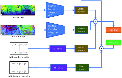
Figure 5: Use IMU only as feature.

Table 2: Comparison among different ways to preprocess imu and whether using imu.

$t_{rel}(\%)$	00	01	02	03	04	05	06	07	08	09	10	trainavg	testavg
imu(w preprocess)	1.50	3.44	1.33	x	0.94	0.98	0.90	1.00	1.63	2.24	1.83	1.58	2.03
imu(w/o preprocess)	1.35	3.56	1.57	x	1.07	1.21	1.03	0.90	1.59	2.46	1.87	1.66	2.17
noimu	1.33	3.40	1.53	1.43	1.26	1.22	1.19	0.97	1.92	3.87	2.69	1.89	3.28
$r_{rel}(^{\circ}/100m)$	00	01	02	03	04	05	06	07	08	09	10	trainavg	testavg
imu(w preprocess)	0.70	0.99	0.59	x	0.78	0.56	0.45	0.54	0.78	1.13	1.14	0.76	1.14
imu(w/o preprocess)	0.67	1.01	0.69	x	0.63	0.68	0.56	0.60	0.71	1.13	1.28	0.80	1.20
noimu	0.69	0.97	0.68	1.04	0.73	0.66	0.64	0.58	0.78	1.67	1.97	0.95	1.82

As mentioned earlier, IMU can greatly improve the accuracy of odometry, but the role played by different IMU utilization methods is also different. If only use IMU to extract features through the network, and directly merge with the feature of the point clouds, the effect is limited (see Fig. 5). Our method uses IMU and LSTM network to estimate a relative initial pose, project vertex image and normal vector image of the original current frame, and then send the projection images into the point clouds feature extraction network, so that the IMU can not only have a direct connection with the final odometry estimate network, but also make the coordinate of two consecutive frames closer. The comparison is shown in Table. 2.

4.4.2 Different operations to obtain the rotation and translation features

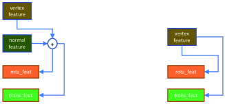
Figure 6: The network structure of learning translation and rotation features from concatenated vetex and normal features simultaneously (left) and the network structure without the normal feature (right).

Table 3: Comparison among whether distinguishing features (dist) and whether using normal.

$t_{rel}(\%)$	00	01	02	03	04	05	06	07	08	09	10	trainavg	testavg
imu(w normal, w dist)	1.50	3.44	1.33	x	0.94	0.98	0.90	1.00	1.63	2.24	1.83	1.58	2.03
imu(w normal, w/o dist)	1.45	3.68	2.03	x	0.72	1.11	1.15	0.68	1.67	3.44	1.86	1.78	2.65
imu(w/o normal, w/o dist)	2.54	3.81	4.13	x	0.95	1.77	0.99	1.25	1.93	2.72	2.21	2.23	2.47
noimu(w normal, w dist)	1.33	3.40	1.53	1.43	1.26	1.22	1.19	0.97	1.92	3.87	2.69	1.89	3.28
noimu(w normal, w/o dist)	1.49	3.95	2.49	2.27	0.88	1.19	0.90	1.47	2.02	4.93	4.34	2.36	4.64
noimu(w/o normal, w/o dist)	1.63	4.96	2.99	2.36	2.15	1.31	1.31	1.51	1.89	5.75	6.11	2.91	5.93
$r_{rel}(^{\circ}/100m)$	00	01	02	03	04	05	06	07	08	09	10	trainavg	testavg
imu(w normal, w dist)	0.70	0.99	0.59	x	0.78	0.56	0.45	0.54	0.78	1.13	1.14	0.76	1.14
imu(w normal, w/o dist)	0.65	1.04	0.96	x	0.53	0.56	0.58	0.46	0.64	1.45	1.15	0.80	1.30
imu(w/o normal, w/o dist)	1.31	1.05	1.60	x	0.52	0.88	0.48	0.87	0.93	1.15	1.21	1.00	1.18
noimu(w normal, w dist)	0.69	0.97	0.68	1.04	0.73	0.66	0.64	0.58	0.78	1.67	1.97	0.95	1.82
noimu(w normal, w/o dist)	0.88	1.24	1.20	1.38	0.66	0.70	0.58	1.03	0.95	1.92	2.06	1.15	1.99
noimu(w/o normal, w/o dist)	0.90	1.48	1.37	1.49	1.38	0.79	0.73	1.08	0.93	2.31	2.73	1.38	2.52

The normal vector contains the relationship between a point and its surrounding points, and can be used as feature of pose estimation just like the point itself. Through the calculation formula of the normal vector, we can know that the change of the normal vector is only related to the orientation, and the translation will not bring about the change of the normal vector. Therefore, we only use the feature of the point to estimate the translation. We compare the original method with the two strategies of not using normal vectors as the network input and not distinguishing feature of the normals and points (see Fig. 6). The comparison is shown in Table. 3.

4.4.3 Attention

Table 4: Comparison among whether using attention module.

$t_{rel}(\%)$	00	01	02	03	04	05	06	07	08	09	10	trainavg	testavg
imu(w attention)	1.50	3.44	1.33	x	0.94	0.98	0.90	1.00	1.63	2.24	1.83	1.58	2.03
imu(w fc+activation)	1.19	3.49	1.48	x	0.83	0.95	0.64	0.91	1.49	3.21	1.54	1.57	2.38
noimu(w attention)	1.33	3.40	1.53	1.43	1.26	1.22	1.19	0.97	1.92	3.87	2.69	1.89	3.28
noimu(w fc+activation)	1.65	3.59	1.67	1.88	0.87	1.34	1.10	1.23	1.76	6.64	3.25	2.27	4.95
$r_{rel}(^{\circ}/100m)$	00	01	02	03	04	05	06	07	08	09	10	trainavg	testavg
imu(w attention)	0.70	0.99	0.59	x	0.78	0.56	0.45	0.54	0.78	1.13	1.14	0.76	1.14
imu(w fc+activation)	0.62	0.97	0.64	x	1.02	0.54	0.42	0.55	0.70	1.20	1.07	0.77	1.13
noimu(w attention)	0.69	0.97	0.68	1.04	0.73	0.66	0.64	0.58	0.78	1.67	1.97	0.95	1.82
noimu(w fc+activation)	0.77	0.99	0.67	1.10	0.70	0.67	0.48	0.80	0.80	2.36	2.07	1.04	2.21

After extracting the features of the vertex map and the normal map, we add an additional self-attention module to improve the accuracy of pose estimation. The attention module can self-learn the importance of features, and give higher weight to more important features. We verify its effectiveness by comparing the result of the model which replaces the self-attention module with a single FC layer with activation function (as formula (12)). The comparison is show in Table. 4.

$$out=tanh(W_{2}(tanh(W_{1}x+b_{1}))+b_{2}).$$ (12)

4.4.4 Loss function

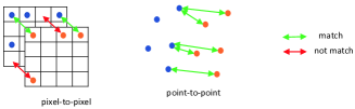
Figure 7: Matching points search strategy of Cho et al.(pixel-to-pixel), our and Nubert et al.(point-to-point).

Table 5: Comparison among different loss functions and matching point search strategy.

$t_{rel}(\%)$	00	01	02	03	04	05	06	07	08	09	10	trainavg	testavg
imu(w point-to-plane))+point-to-point	1.50	3.44	1.33	x	0.94	0.98	0.90	1.00	1.63	2.24	1.83	1.58	2.03
imu(w/o point-to-plane)+point-to-point	2.27	4.33	2.24	x	1.59	1.70	1.26	1.29	1.87	2.04	2.07	2.07	2.06
imu(w point-to-plane)+pixel-to-pixel	2.14	4.36	2.29	x	1.65	1.66	1.17	1.36	1.73	2.95	2.28	2.16	2.61
noimu(w point-to-plane)+point-to-point	1.33	3.40	1.53	1.43	1.26	1.22	1.19	0.97	1.92	3.87	2.69	1.89	3.28
noimu(w/o point-to-plane)+point-to-point	1.46	3.44	1.67	1.91	0.92	1.00	1.11	1.36	1.81	4.72	2.78	2.02	3.75
noimu(w point-to-plane))+pixel-to-pixel	2.76	4.43	2.73	2.07	1.71	1.50	1.32	1.32	1.95	3.68	3.65	2.47	3.67
$r_{rel}(^{\circ}/100m)$	00	01	02	03	04	05	06	07	08	09	10	trainavg	testavg
imu(w point-to-plane))+point-to-point	0.70	0.99	0.59	x	0.78	0.56	0.45	0.54	0.78	1.13	1.14	0.76	1.14
imu(w/o point-to-plane)+point-to-point	1.01	1.12	0.98	x	0.96	0.82	0.62	0.78	0.86	1.14	1.19	0.95	1.16
imu(w point-to-plane)+pixel-to-pixel	0.96	1.11	0.96	x	0.98	0.83	0.58	0.83	0.87	1.52	1.27	0.99	1.39
noimu(w point-to-plane)+point-to-point	0.69	0.97	0.68	1.04	0.73	0.66	0.64	0.58	0.78	1.67	1.97	0.95	1.82
noimu(w/o point-to-plane)+point-to-point	0.73	0.99	0.70	1.34	0.69	0.58	0.49	0.85	0.76	1.85	1.84	0.98	1.85
noimu(w point-to-plane))+pixel-to-pixel	1.10	1.16	1.11	1.40	1.03	0.76	0.62	0.78	0.89	1.56	2.05	1.13	1.80

Cho et al. [5] adopt the strategy of using the points with the same pixel in last and current vertex map as the matching points. Although the calculation speed is fast, the matching points found in this way are likely to be incorrect. Therefore, we and Nubert et al. [15] imitate ICP algorithm, using the nearest neighbor as the matching point(see Fig. 7). Although we use the same loss functions and the same matching point search strategy (nearest neighbor) as Nubert et al. [15], we search in the entire point clouds space, and maintain the number of points in search space not too large by removing most of the ground points and operating voxel grids downsample on point clouds. The number of points even is only 1/3 of the points sampled by the 2D projection which used in [15]. Table. 5 shows the necessity of two loss parts and strategy of searching matching points in the entire point clouds.

5 Conclusion

In this paper, we proposed UnDeepLIO, an unsupervised learning-based odometry network. Different from other unsupervised lidar odometry methods, we additionally used IMU to assist odometry task. There have been already many IMU and lidar fusion algorithms in the traditional field for odometry, and it has become a trend to use the information of both at the same time. Moreover, we conduct extensive experiments on kitti dataset and experiments verify that our method is competitive with the most advanced methods. In ablation study, we validated the effectiveness of each component of our model. In the future, we will study how to incorporate mapping steps into our network framework and conduct online tests.

References

- [1] Arun, K.S., Huang, T.S., Blostein, S.D.: Least-squares fitting of two 3-d point sets. TPAMI 9(5), 698–700 (1987)
- [2] Behley, J., Stachniss, C.: Efficient surfel-based slam using 3d laser range data in urban environments. In: Robotics: Science and Systems. vol. 2018 (2018)
- [3] Bentley, J.L.: Multidimensional binary search trees used for associative searching. Communications of the ACM 18(9), 509–517 (1975)
- [4] Cho, Y., Kim, G., Kim, A.: Deeplo: Geometry-aware deep lidar odometry. arXiv preprint arXiv:1902.10562 (2019)
- [5] Cho, Y., Kim, G., Kim, A.: Unsupervised geometry-aware deep lidar odometry. In: ICRA. pp. 2145–2152. IEEE (2020)
- [6] Fischler, M.A., Bolles, R.C.: Random sample consensus: a paradigm for model fitting with applications to image analysis and automated cartography. Communications of the ACM 24(6), 381–395 (1981)
- [7] Geiger, A., Lenz, P., Urtasun, R.: Are we ready for autonomous driving? the kitti vision benchmark suite. In: CVPR. pp. 3354–3361. IEEE (2012)
- [8] He, K., Zhang, X., Ren, S., Sun, J.: Deep residual learning for image recognition. In: CVPR. pp. 770–778 (2016)
- [9] Hochreiter, S., Schmidhuber, J.: Long short-term memory. Neural computation 9(8), 1735–1780 (1997)
- [10] Javanmard-Gh., A.: Deeplio: Deep lidar inertial odometry. https://github.com/ArashJavan/DeepLIO (2020)
- [11] Kingma, D.P., Ba, J.: Adam: A method for stochastic optimization. In: ICLR (2015)
- [12] Li, Q., Chen, S., Wang, C., Li, X., Wen, C., Cheng, M., Li, J.: Lo-net: Deep real-time lidar odometry. In: CVPR. pp. 8473–8482 (2019)
- [13] Li, Z., Wang, N.: Dmlo: Deep matching lidar odometry. In: IROS (2020)
- [14] Low, K.L.: Linear least-squares optimization for point-to-plane icp surface registration. Chapel Hill, University of North Carolina 4(10), 1–3 (2004)
- [15] Nubert, J., Khattak, S., Hutter, M.: Self-supervised learning of lidar odometry for robotic applications. In: ICRA (2021)
- [16] Paszke, A., Gross, S., Massa, F., Lerer, A., Bradbury, J., Chanan, G., Killeen, T., Lin, Z., Gimelshein, N., Antiga, L., et al.: Pytorch: An imperative style, high-performance deep learning library. In: NIPS (2019)
- [17] Pauly, M.: Point primitives for interactive modeling and processing of 3D geometry. Hartung-Gorre (2003)
- [18] Qi, C.R., Su, H., Mo, K., Guibas, L.J.: Pointnet: Deep learning on point sets for 3d classification and segmentation. In: CVPR. pp. 652–660 (2017)
- [19] Segal, A., Haehnel, D., Thrun, S.: Generalized-icp. Robotics: science and systems 2(4), 435 (2009)
- [20] Shan, T., Englot, B.: Lego-loam: Lightweight and ground-optimized lidar odometry and mapping on variable terrain. In: IROS. pp. 4758–4765. IEEE (2018)
- [21] Velas, M., Spanel, M., Hradis, M., Herout, A.: Cnn for imu assisted odometry estimation using velodyne lidar. In: ICARSC. pp. 71–77. IEEE (2018)
- [22] Wang, W., Saputra, M.R.U., Zhao, P., Gusmao, P., Yang, B., Chen, C., Markham, A., Trigoni, N.: Deeppco: End-to-end point cloud odometry through deep parallel neural network. In: IROS (2019)
- [23] Xu, Y., Huang, Z., Lin, K.Y., Zhu, X., Shi, J., Bao, H., Zhang, G., Li, H.: Selfvoxelo: Self-supervised lidar odometry with voxel-based deep neural networks. In: CoRL (2020)
- [24] Zhang, J., Singh, S.: Loam: Lidar odometry and mapping in real-time. Robotics: Science and Systems 2(9) (2014)
- [25] Zheng, C., Lyu, Y., Li, M., Zhang, Z.: Lodonet: A deep neural network with 2d keypoint matching for 3d lidar odometry estimation. In: ACM MM. pp. 2391–2399 (2020)