Ghost Loss to Question the Reliability of Training Data

Abstract

Supervised image classification problems rely on training data assumed to have been correctly annotated; this assumption underpins most works in the field of deep learning. In consequence, during its training, a network is forced to match the label provided by the annotator and is not given the flexibility to choose an alternative to inconsistencies that it might be able to detect. Therefore, erroneously labeled training images may end up “correctly” classified in classes which they do not actually belong to. This may reduce the performances of the network and thus incite to build more complex networks without even checking the quality of the training data. In this work, we question the reliability of the annotated datasets. For that purpose, we introduce the notion of ghost loss, which can be seen as a regular loss that is zeroed out for some predicted values in a deterministic way and that allows the network to choose an alternative to the given label without being penalized. After a proof of concept experiment, we use the ghost loss principle to detect confusing images and erroneously labeled images in well-known training datasets (MNIST, Fashion-MNIST, SVHN, CIFAR10) and we provide a new tool, called sanity matrix, for summarizing these confusions.

How to cite this work? This is the authors’ preprint version of a paper published in IEEE Access in 2020. Please cite it as follows: A. Deliège, A. Cioppa and M. Van Droogenbroeck, "Ghost Loss to Question the Reliability of Training Data", in IEEE Access, vol. 8, pp. 44774-44782, 2020, doi: 10.1109/ACCESS.2020.2978283.

1 Introduction

Large amounts of publicly available labeled training images are at the root of some of the most impressive breakthroughs made in deep supervised learning in recent years. From several thousands of images (e.g. MNIST [9], CIFAR10 [8], SVHN [12]) to millions (e.g. ImageNet [3], Quick Draw [5]), such datasets are often used as a basis upon which new techniques are developed and compared to keep track of the advances in the field. However, both the collection and the annotation of such large datasets can be time-consuming and are thus often computer-aided, if not completely automated. This results in the production of datasets that have not been manually checked by humans, which is a practically impossible task in many cases. Consequently, one cannot exclude the possibility that annotation errors or irrelevant images are present in the final datasets released publicly. These are generally randomly split into a training set from which a network learns to classify the images and a test set used to measure the performances of the network on unseen images, both of which may thus contain misleading images. By construction of these two sets, some errors can be consistent between them, which makes them difficult to detect and may reduce the performances when the network is deployed in a real application. The other errors in the training and test sets contribute to decrease the performances on the test set, which might thus appear artificially challenging since top performances are out of reach. In all cases, rather than questioning the reliability of the data, the usual approach to improve the results is to design larger and deeper networks, or networks that are able to deal with label noise [4, 13]. We believe that a careful prior examination of the dataset is more important, since it could greatly help solving the classification task.

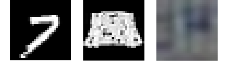
Figure 1: Training images of MNIST, Fashion-MNIST, SVHN officially labeled as “4”, “shirt”, “9”. The ghost loss helps detecting such problematic training images.

In this work, we introduce the principle of a “ghost loss” to help analyzing four widely used training sets (MNIST, Fashion-MNIST [16], SVHN, CIFAR10) without requiring a manual inspection of thousands of images. First, we detail the notion of ghost loss, which allows the network to choose an alternative to the label provided by the annotator without being penalized during the training phase. This way, when an image is mislabeled, the network is given the possibility to report that it has detected a potentially misleading image. This is done by zeroing out the loss associated with the "most likely" wrong prediction. A proof of concept experiment is presented in order to properly illustrate its usefulness in a basic case. Then, the ghost loss is used to examine the four previously mentioned training sets. We show that some confusions are indeed present, such as those displayed in Figure 1, and we define a new tool, called sanity matrix, to summarize them. We also show that different types of confusions can be detected. They may originate from annotation errors, irrelevant images, or from images that are intrinsically ambiguous and deserve multiple labels. Let us emphasize that, in this work, we focus on using the notion of ghost to analyze datasets. Further developments will be envisioned in future works. Codes will be released in due time.

2 Related work

Dealing with label noise in the context of supervised machine learning is a well-known issue that challenges researchers since the early developments of classifiers, as detailed in [1]. A vast corpus of techniques has been developed, most of which are listed in a recent exhaustive survey [7], where even the latest methods related to general deep learning algorithms are indexed. Interestingly, in [7], authors propose to classify techniques for handling label noise into six (possibly overlapping) categories. In the following, we briefly describe those that are related to our work.

1. Loss functions. Many works focus on designing loss functions that are more robust to label noise than usual losses, such as [18, 17]. In this category, our work is somehow close to [18], which allows the network to refrain from making a prediction at the cost of receiving a penalty. A difference is that in our case, the network has to make a prediction for each class, but we zero out the loss for one of them. This principle is also close to [19], where the loss ignores the training samples with the largest loss values. However, in our case, only the prediction for one class is ignored (almost based on the loss value as well), not the training sample itself. Besides, works focusing on designing robust loss functions generally do not attempt to identify which training samples are mislabeled, contrary to our work.

2. Consistency. Some works (including ours) are based on the hypothesis that samples of the same class share similar features. Hence, the features of a mislabeled sample are not correlated with the features of the samples of its assigned class. For instance, this idea is used in [20] through a Siamese network trained to predict the similarity between faces, via the distance between their features in a lower-dimensional space. In comparison, our work can be seen as comparing the features with a fixed prototype of reference and thus does not need pairwise training.

3. Data re-weighting. These techniques attempt to down-weight the importance of the training samples that might be mislabeled during the learning process. The method previously mentioned [19] is a particular case of this class, as some training samples are assigned a null weight. In our case, a null weight is assigned on the predictions level, hence a training sample is never completely discarded. In [21], authors propose to re-weight the gradients computed from the predictions of the network to accomodate for the noisy labels. The weights depend on the type of loss function used and on the prediction values themselves. In our case, zeroing out the loss for one prediction also modifies the gradients but is loss-agnostic.

4. Label cleaning. Some works attempt to clean the labels on-the-fly during training. For instance, [22] use transfer learning strategies to compare the features of an image with features of reference (as for method 2.) before deciding to accept the label as is or to modify it. However, this method requires a clean subset of data, which requires careful prior examination. Our work does not require that and does not modify the labels directly. It rather helps analyzing the dataset after a network has been trained.

Finally, let us note that no paper actually provides a way to assess the quality of a dataset as we do in this work, nor really aims at exposing mislabeled images. Besides, related works focus on reaching high performances, while we intentionnally reduce the discriminative power of our network to achieve our objectives.

3 Method

We assume to have a $K$-classes classification network which outputs, for each input image, $K$ feature vectors of a given size $n$. The $k\text{-th}$ feature vector is associated with the $k\text{-th}$ class and can be seen as a vector of class-specific features used to compute a prediction value $y_{\text{pred},\,k}$ that determines whether the input image belongs to that $k\text{-th}$ class or not. For instance, in [14], the length of the $k\text{-th}$ feature vector is used to compute $y_{\text{pred},\,k}$, but other choices can be made, such as its distance from a fixed reference vector, as in [2]. Most standard architectures can be seen as using $n=1$ and the $k$-th “feature vector” is $y_{\text{pred},\,k}$ itself. As for any network, the prediction vector $y_{\text{pred}}$ made of the $K$ values obtained from the $K$ feature vectors is compared with a one-hot encoded ground-truth vector $y_{\text{true}}$ through a loss function $L(y_{\text{true}},y_{\text{pred}})$. The $k\text{-th}$ component of $y_{\text{true}}$ is noted $y_{\text{true},\,k}$. We assume that the loss can be decomposed as the sum of $K$ losses, in a multiple binary classifiers fashion:

$$L(y_{\text{true}},y_{\text{pred}})=\sum_{k=1}^{K}y_{\text{true},\,k}\,L_{1}^{k}(y_{\text{pred},\,k})\\ +(1-y_{\text{true},\,k})\,L_{0}^{k}(y_{\text{pred},\,k})\enspace\mbox{,}$$ (1)

where $L_{1}^{k}(y_{\text{pred},\,k})$ (resp. $L_{0}^{k}(y_{\text{pred},\,k})$) is the loss generated by $y_{\text{pred},\,k}$ when $y_{\text{true},\,k}=1$ (resp. $0$). One generally chooses the same $L_{1}^{k}(.)$ for all the values of $k$, up to class-specific multiplicative factors used to handle class imbalance; the same principle holds for $L_{0}^{k}(.)$. For example, in the case of the categorical cross-entropy loss preceded by a softmax activation, one has $n=1$, $L_{1}^{k}(.)=-\log(.)$ for all $k$ and $L_{0}^{k}(.)=0$ for all $k$.

In this configuration, the network is not allowed to question the true labels $y_{\text{true}}$ provided by the annotator. Indeed, in the back-propagation process, in order to minimize the loss, it is forced to update all the feature vectors towards given target zones, i.e. zones where their associated prediction values are close to (or far from) target values such as $0$, $0.5$, $1$, … . However, this can be problematic in some cases. For example, if an image of a horse is erroneously labeled as a truck, then the network has to find a way to produce a feature vector “horse” whose prediction value indicates that the image is not of a horse and a feature vector “truck” whose prediction value indicates that the image represents a truck. Now, considering that the network has many other training images of horses and trucks correctly labeled at its disposal, it will be able to detect their characteristics and to produce discriminative “horse” feature vectors for horses and “truck” feature vectors for trucks. Therefore, despite being labeled as truck, the erroneously labeled image of a horse is still likely to exhibit a horse feature vector giving a prediction value which is much “more significant” than the prediction values of the airplane, frog, or any other class. By “more significant”, we mean closer to the aforementioned target value, e.g. “more likely” in a probabilistic setting. In such a case, it would be more appropriate not to penalize the horse feature vector, which conveniently already appears to be associated with “the most significant non true class”. This is the motivation behind the present work.

Definitions.

In order to give the network the capacity to opt for an alternative to the labels provided by the annotator, we introduce the notions of “ghost feature vector” and “ghost loss”. The ghost feature vector of an image is the feature vector corresponding to the most significant prediction value among the $K-1$ feature vectors not corresponding to the feature vector of the true class. The contribution to $L$ engendered by the ghost feature vector is zeroed out and is called a ghost loss:

$$L_{0}^{k_{\text{ghost}}}(y_{\text{pred},\,k_{\text{ghost}}})\leftarrow 0\enspace\mbox{.}$$ (2)

This means that, during the training phase, the ghost feature vector is not forced to target any particular zone, and is not involved in the update of the weights from one batch to the next; it is essentially invisible in the back-propagation, hence its name. The concept of ghost vector is illustrated in Figure 2.

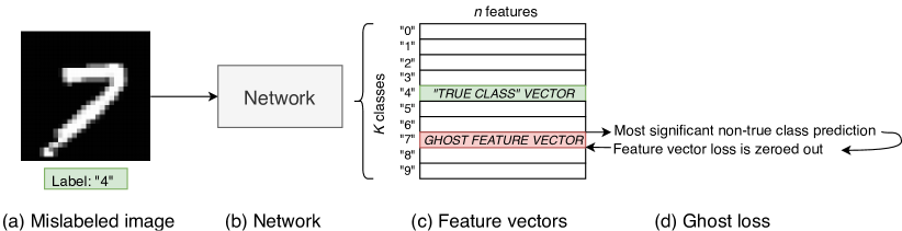
Figure 2: Illustration of the ghost feature vector and ghost loss principle. A training image (a) of a digit “7” is mislabeled as “4”. The network (b) outputs feature vectors (c). The feature vector leading to the most significant prediction value among those different from the feature vector “4” is selected as the ghost feature vector. Here, the feature vector “7” is expected to be the ghost feature vector. The loss generated by this ghost feature vector is then zeroed out (d).

From an implementation point of view, training a network with ghost feature vectors and a ghost loss is similar to training it without, only the loss defined in Equation 1 needs to be adjusted. Given a one-hot encoded label $y_{\text{true}}$ and the prediction vector of the network $y_{\text{pred}}$, the loss $L_{\text{ghost}}$ can be written as:

$$L_{\text{ghost}}(y_{\text{true}},y_{\text{pred}})=\sum_{k=1}^{K}y_{\text{true},\,k}\,L_{1}^{k}(y_{\text{pred},\,k})\\ +{\color[rgb]{0,0,1}\gamma}_{{\color[rgb]{0,0,1}k}}(1-y_{\text{true},\,k})\,L_{0}^{k}(y_{\text{pred},\,k})\enspace\mbox{,}$$ (3)

where $\gamma_{k}=0$ if $k=k_{\text{ghost}}$, and $\gamma_{k}=1$ otherwise.

Two important characteristics are thus associated with a ghost feature vector: its class $k_{\text{ghost}}$, which is always one of the $K-1$ classes not corresponding to the true class of the input image, which we call the ghost class, and its associated prediction value $y_{\text{pred},\,k_{\text{ghost}}}$, that we call ghost prediction. The ghost class $k_{\text{ghost}}$ of an image is obtained in a deterministic way, at each epoch, as the class of the most significant non true class prediction; it is not a Dropout [15], nor a learned Dropout variant (as e.g. [10]). The ghost class of an image can change from one epoch to the next as the network trains. Ideally, a ghost feature vector will have a significant ghost prediction when its ghost class is a plausible alternative to the true class or if the image deserves an extra label, and will not otherwise. The evolution of a ghost feature vector during the training is dictated by the overall evolution of the network.

Subsequently, in the situation described above, at the end of the training, the image of a horse labeled as a truck should actually display two significant prediction values: one for the feature vector corresponding to the “truck” class since the network was forced to do so, and one for the feature vector corresponding to the “horse” class. Indeed, the network probably selected the “horse” feature vector as ghost feature vector because the image displays the features needed to identify a horse and it was not forced to give it a non significant prediction value. Looking at the images with significant prediction values at the end of the training allows to detect the images for which the network suspects an error in the label, or for which assigning two labels might be relevant.

We can derive a new tool from the notions defined above that helps aggregating information on the number of training images that might be considered as suspicious. This tool takes the form of a matrix, which we call “sanity matrix”, in which the counts of the pairs (true class, ghost class) are reported when the ghost prediction is sufficiently significant with respect to a given threshold.

Let us note that the ghost loss principle should not be used along with the categorical cross-entropy loss preceded by a softmax activation. Indeed, in such a case, the use of $L_{0}^{k}$ is obsolete since the cross-entropy loss can be seen as a particular case of Equation 1 in which $L_{1}^{k}(.)=-\log(.)$ for all $k$ and $L_{0}^{k}(.)=0$ for all $k$. Therefore, the introduction of $\gamma_{k}$ in Equation 3 has no impact on the loss.

4 Experiments

4.1 Network used

The network used in the following experiments comes from [2]. It is a simplified and adapted version of the network introduced in [14]. The network that we use for the experiments is represented in Figure 3 and is composed of the following elements, as in [2].

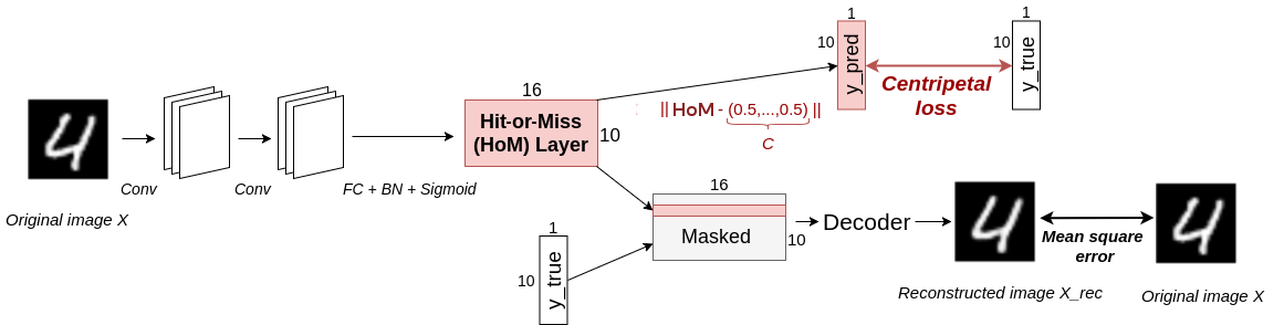
Figure 3: Graphical representation of the network structure used for the experiments in this paper.

First, two $9\times 9$ (with strides (1,1) then (2,2)) convolutional layers with 256 channels and ReLU activations are applied, to obtain feature maps. Then, we use a fully connected layer to a $K\times n$ matrix, followed by a BatchNormalization and an element-wise sigmoid activation, which produces what we call the Hit-or-Miss (HoM) layer composed of $K$ feature vectors of size $n$. We set $n=16$ as in [2]. The Euclidean distance with the central feature vector $C:(0.5,\,\ldots,\,0.5)$ is computed for each feature vector of HoM, which gives the prediction vector of the model $y_{\text{pred}}$. This is done such that, for a given image, the feature vector of the true class is close to $C$ (prediction value $y_{\text{pred},\,k}$ close to $0$) and the feature vectors of the other classes are far from $C$ (prediction value $y_{\text{pred},\,k}$ close to $\sqrt{n}/2=2$). In this spirit, regarding the loss defined in Equation 3, we choose $L_{0}^{k}(y_{\text{pred},\,k})$ and $L_{1}^{k}(y_{\text{pred},\,k})$ such that, for all $k$:

$$L_{0}^{k}(y_{\text{pred},\,k})=0.5\,\max(0,y^{2}_{\text{pred},\,k}-1.9\,y_{\text{pred},\,k}+0.9)\enspace\mbox{,}$$ (4)

and

$$L_{1}^{k}(y_{\text{pred},\,k})=\max(0,y^{2}_{\text{pred},\,k}-0.1\,y_{\text{pred},\,k})\enspace\mbox{.}$$ (5)

The loss associated with the feature vector of the true class ($L_{1}$) and the loss associated with the other feature vectors ($L_{0}$) are represented in Figure 4 in the case where $n=2$. The zones where the losses equal zero are called hit zones (for $L_{1}$) and miss zones (for $L_{0}$) and are reached when $y_{\text{pred},\,k}<0.1$ and $y_{\text{pred},\,k}>0.9$ respectively. The network has to try to place the feature vector of the true class in the hit zone of its own space, and the feature vectors of the other classes in the miss zones of their respective spaces. For the classification task, the label predicted by our network is the index of the lowest entry of $y_{\text{pred}}$.

Besides, a decoder follows the HoM layer to help visualize the results, as represented in Figure 3, but is not mandatory for the ghost loss to work. During the training, all the feature vectors of HoM are masked (set to $0$) except the one related to the true class, then they are concatenated and sent to the decoder, which produces an output image $X_{\text{rec}}$, that aims at reconstructing the initial image $X$. The decoder consists in two fully connected layers of size $512$ and $1024$ with ReLU activations, and one fully connected layer to a tensor with the same dimensions as the input image, with a sigmoid activation. The quality of the reconstructed image $X_{\text{rec}}$ is evaluated through the mean squared error with $X$. This error is down-weighted with a multiplicative factor $\alpha$ set to $0.392$ and is then added to $L_{\text{ghost}}$ to produce the final composite loss.

In the following, the networks are run during $250$ epochs with the Adam optimizer with a constant learning rate of $0.001$, with batches of $128$ images.

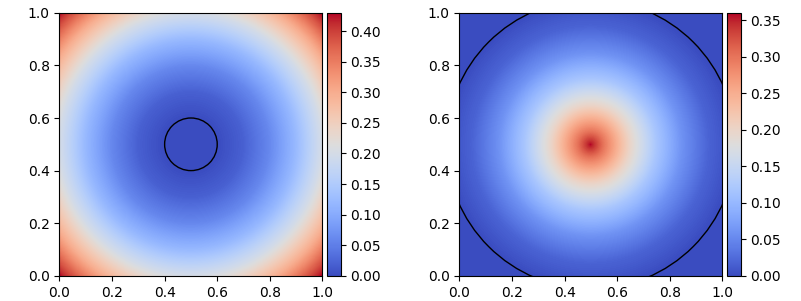
(a)(b)

Figure 4: Illustration of the type of loss used in our experiments, in the 2-dimensional case ($n=2$). The loss associated with the feature vector of the true class is given by plot (a). The loss-free hit zone is the area within the black circle. The loss generated by the other feature vectors is given by plot (b). The loss-free miss zone is the area outside the black circle.

4.2 Proof of concept

In order to illustrate the principle of the ghost loss detailed above, we perform the following “proof of concept” experiment. We consider the MNIST training set for clearer visual representations. We assign the label “0” to the first image, which actually depicts a digit “5”, as shown in Figure 5. Then, we run our network without using the ghost feature vectors nor the ghost loss. At the end of the training, we compute the prediction values of that image. In the present setting, let us recall that we expect small prediction values for the more legitimate classes and large prediction values for the non plausible classes. As expected, the lowest prediction value corresponds to the class “0”, with $y_{\text{pred},\,0}=0.22$; the image is thus ‘correctly’ classified by the network, which is an obvious case of overfitting.

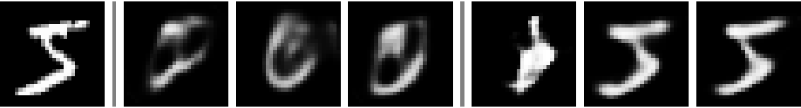
(1)  (2)  (3)      (4)    (5)     (6)      (7)

Figure 5: (1) Initial image of a digit “5”, that we mislabel as “0”. Then, the reconstructions from feature vector “0” when no ghost feature vector is allowed (2), one ghost feature vector is allowed for this image only (3), one ghost feature vector is allowed for each training image (4). None of the reconstructions based on the feature vector of the “true class 0” matches the initial image. Then, the corresponding reconstructions from feature vector “5” (5,6,7). When ghost feature vectors are allowed, the network is able to reconstruct the initial image from the feature vector “5”, which corresponds to a non-true class, while it is not the case when no ghost feature vector is allowed. This indicates that the introduction of ghost feature vectors enables the network to learn representative features of non-true classes, when necessary.

The second lowest prediction value corroborates our hypothesis since it corresponds to the class “5”, with $y_{\text{pred},\,5}=1.10$. Given that $y_{\text{pred},\,5}>0.9$, the network managed to place the feature vector “5” in the miss zone, despite the fact that the image actually represents a “5”. The decoder can be used to visualize the information contained in feature vectors “0” and “5”, as shown in Figure 5. It appears that, even though the image is correctly classified as a “0” and the network was trained to reconstruct the image from feature vector “0”, the reconstruction based on feature vector “0” does not match the initial image. Of course, the reconstruction based on feature vector “5” does not represent a proper “5” either. The experiment is repeated several times. In total, $20$ runs of our network are performed, consistently leading to similar conclusions, as it can be visualized in Figure 6(a).

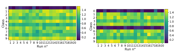
(a) no ghost feature vector(b) one ghost feature vector

Figure 6: Prediction values of the $20$ runs for the erroneously labeled image when (a) no ghost feature vector is allowed (the network is confident that the image is a “0” and nothing else), and when (b) a ghost feature vector is allowed for this image. For (b), the network consistently suspects that the image might actually display the digit “5”.

Then, we run the same experiment, but we allow one ghost feature vector via the ghost loss only for that erroneously labeled image. We do not impose that this ghost feature vector has to be feature vector “5”; we simply allow the network, at each epoch, to choose one feature vector per image that will not generate any loss. At the end of the training, we compute the prediction values of that image. In this case, we obtain $y_{\text{pred},\,0}=0.10$ and $y_{\text{pred},\,5}=0.14$, which indicates that the network does not trust the label provided since feature vector “5”, obviously chosen as ghost feature vector, is close to the hit zone (prediction $<0.1$). All the remaining feature vectors are in the miss zone (prediction $>0.9$) as expected. In this case, reconstructing the image from the information contained in feature vector “0” is again far from the initial image, while the reconstruction from feature vector “5” is close to the initial image (see Figure 5). Again, the experiment is run $20$ times. It appears that the ghost feature vector selected by the network is feature vector “5” for the $20$ runs and that it is consistently close to (and occasionally inside) the hit zone, with a mean prediction value of $0.17$, as reflected in Figure 6(b). In fact, the feature vector “5” is even closer to the hit zone than the feature vector “0” in $10$ runs.

Finally, we run the same experiment, but we allow one ghost feature vector per training image, as if we were in the realistic situation of not being aware of that erroneous label. The results are similar to the previous case. The reconstruction from feature vector “0” is bad while the one from feature vector “5” is good (see Figure 5). Among $20$ runs, the ghost feature vector is always feature vector “5”, with a mean prediction value of $0.14$, and it is closer to the hit zone than the feature vector “0” in $7$ runs.

4.3 Automatic detection of abnormalities in well-known training sets

In the following experiments, we allow one ghost feature vector for each image of the training set via the ghost loss. This enables us to analyze the dataset and detect possibly mislabeled images by examining the ghost feature vectors, their associated ghost classes and ghost predictions. Let us recall that, for each experience, we trained our network $20$ times, which gives us as many models, and we examine the $20$ ghost feature vectors associated with each image by these models.

4.3.1 Analysis of MNIST

First, we study the agreement between the models about the $20$ ghost classes selected for each image on the MNIST dataset, which is composed of images representing handwritten digits from “$0$” to “$9$”. For that purpose, we examine the distribution of the number of different ghost classes given to each image. It appears that the $20$ models all agree on the same ghost class for $16.859$ training images, which represents $28\%$ of the training images. These images have a pair (true class, ghost class) and their distribution suggests that some pairs are more likely to occur, such as $(3,5)$ for $2333$ images, $(4,9)$ for $2580$ images, $(7,2)$ for $1360$ images, $(9,4)$ for $2380$ images, which gives a glimpse of the classes that might be likely to be mixed up by the models. Confusions may occur because of errors in the true labels, but since these numbers are obtained on the basis of an agreement of $20$ models trained from the same network structure, this may also indicate the limitations of the network structure itself in its ability to identify the different classes. However, a deeper analysis is needed to determine if these numbers indicate a real confusion or not, that is, which of them make hits (ghost prediction $<0.1$) and which do not. We can examine if the $20$ models agree on the ghost predictions of the corresponding feature vectors. For that purpose, for each image, we compute the mean and the standard deviation of its $20$ ghost predictions. An interesting and important observation is that when the mean ghost prediction gets closer to the hit zone threshold $m$, then the standard deviation decreases, which indicates that all the models tend to agree on the fact that a hit is needed.

We can now narrow down the analysis to the images that are the most likely to be mislabeled, that is, those with a mean ghost prediction smaller than $0.1$; there are $71$ such images left, which provides the sanity matrix given in Table 1. From the expected confusions mentioned above, that is $(3,5)$, $(4,9)$, $(7,2)$, $(9,4)$, we can see that $(7,2)$ is not so much represented in the present case, while $(1,7)$ and $(7,1)$ subsisted in a larger proportion, and that $(4,9)$ and $(9,4)$ account for almost half of the images. A last refinement to our analysis consists of looking at the number of hits among the $20$ ghost vectors of these $71$ images. It appears that all these images have at least $55\%$ $(11/20)$ of their ghost feature vectors in the hit zone and that more than $75\%$ $(55/71)$ of the images have a hit for at least $75\%$ $(15/20)$ of the models, which indicates that when the ghost prediction is smaller than $0.1$, it is the result of a strong agreement between the models.

		True class
		0	1	2	3	4	5	6	7	8	9
Ghost class	0	0	0	0	0	0	0	0	0	0	0
	1	0	0	0	0	2	0	0	6	0	0
	2	0	0	0	0	0	0	0	1	0	0
	3	0	0	0	0	0	2	0	0	0	0
	4	0	0	0	0	0	0	1	0	0	20
	5	0	0	0	8	0	0	1	0	0	0
	6	0	0	0	0	0	2	0	0	0	0
	7	0	7	2	0	1	0	0	0	0	2
	8	0	0	0	1	0	0	0	0	0	0
	9	0	0	0	1	13	0	0	1	0	0

Table 1: Sanity matrix for MNIST training images having a unique ghost class and their mean ghost prediction smaller than the hit zone threshold.

Finally, the $71$ images, sorted by number of hits, are represented in Figure 7. The number of hits, the ghost class, and the true class are indicated for each image. Some of these images are clearly mislabeled, such as the image with the first $[16,5,3]$ tag and the one with the $[20,7,4]$ tag. Others are terribly confusing by looking almost the same but having different true classes, such as the images with the $[12,2,7]$ and $[18,7,2]$ tags, which explains the ghost classes selected. While pursuing a different purpose, the DropMax technique used in [10] allowed the authors to identify “hard cases” of the training set which are among the $71$ images represented in Figure 7. Some misleading images in the test set, presenting similar errors as those shown in Figure 7, are displayed in e.g.  [11]. All in all, MNIST training set appears to be globally reliable, even though a few images could be either removed or relabeled.

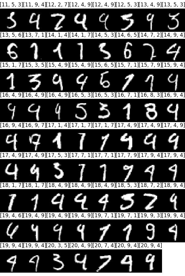
Figure 7: The $71$ images of MNIST training set whose $20$ ghost feature vectors have a mean ghost prediction smaller than the hit zone threshold, sorted by increasing number of hits. A triplet $[\mathtt{a},\mathtt{b},\mathtt{c}]$ indicates that $\mathtt{a}$ hits have been observed in the ghost class $\mathtt{b}$ whereas the true class is $\mathtt{c}$.

4.3.2 Analysis of Fashion-MNIST

Zalando’s Fashion-MNIST dataset is a MNIST-like dataset in the fashion domain. The images are divided in ten classes: T-shirt/top (0), trouser (1), pullover (2), dress (3), coat (4), sandal (5), shirt (6), sneaker (7), bag (8), ankle boot (9). We proceed exactly as above to analyze this dataset with ghost feature vectors. It appears that the $20$ models all agree on the same ghost class for $39074$ training images, which represents $65\%$ of the training images. This large percentage can be seen as a first warning sign of frequent confusions between classes. Among them, $7848$ have a mean ghost prediction smaller than $0.1$, which still represents more than $13\%$ of the training set. The sanity matrix can be found in Table 2 and a few of these images are displayed in Figure 8. Let us also note that $1123$ of them display $20$ hits in their ghost class. These results indicate that the classes of Fashion-MNIST may not be as well separated as in the case of MNIST. For example, from Table 2, it can be inferred that the classes “T-shirt/top” and “shirt” are likely to be mixed up by the network, the same observation holds for “sandal” and “sneaker” or “ankle boot” and “sneaker” quite rightly. Such proposed alternatives are not particularly surprising when looking at the images displayed in Figure 8, which are hardly distinguishable with the naked eye. Interestingly, many “trouser” images have their ghost feature vectors in the “dress” class, which comes from the fact that many images of dresses are simply represented by a white vertical pattern, as for some trousers. These observations raise the question of the quality of the dataset. While it is possible that some confusions can be handled with larger and deeper networks, a visual inspection of the images identified as misleading in this first study reveals that this classification problem might be partially ill-posed, in the sense that several categories could be merged or two labels could be assigned to many images. Alternatively, one can argue that the resolution of the images is simply too low to properly identify the correct class, and that a much more interesting problem would be the classification of higher resolution images of fashion items. In any case, artificial difficulties arise with Fashion-MNIST dataset, which are probably present in the test set as well. Fashion-MNIST may thus not necessarily be used as a “direct drop-in replacement for the original MNIST dataset for benchmarking machine learning algorithms” as openly intended; it may rather serve as a valuable complementary dataset.

		True class
		0	1	2	3	4	5	6	7	8	9
Ghost class	0	0	0	4	45	0	0	994	0	0	0
	1	0	0	0	83	0	0	0	0	0	0
	2	0	0	0	0	138	0	46	0	0	0
	3	35	1004	4	0	156	0	9	0	0	0
	4	0	0	185	33	0	0	95	0	1	0
	5	0	0	0	0	0	0	0	1220	0	13
	6	1131	0	60	0	51	0	0	0	0	0
	7	0	0	0	0	0	1105	0	0	0	801
	8	2	0	0	0	0	0	2	0	0	0
	9	0	0	0	0	0	34	0	597	0	0

Table 2: Sanity matrix for Fashion-MNIST training images having a unique ghost class and their mean ghost prediction smaller than the hit zone threshold. The classes are: T-shirt/top (0), trouser (1), pullover (2), dress (3), coat (4), sandal (5), shirt (6), sneaker (7), bag (8), ankle boot (9).

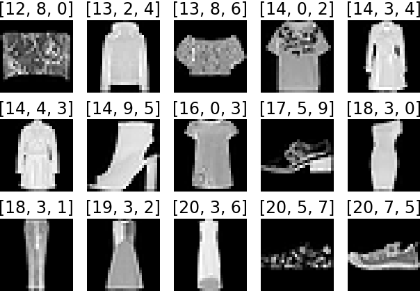
Figure 8: A selection of training images of Fashion-MNIST whose $20$ ghost feature vectors have a mean ghost prediction smaller than the hit zone threshold. The classes are: T-shirt/top (0), trouser (1), pullover (2), dress (3), coat (4), sandal (5), shirt (6), sneaker (7), bag (8), ankle boot (9).

4.3.3 Analysis of SVHN

Following the same process as above, we use ghost feature vectors to analyze the SVHN dataset. It appears that the $20$ models all agree on the same ghost class for $15516$ training images, which represents $21\%$ of the training images. Among them, $121$ have a mean ghost prediction smaller than $0.1$. A few of them are displayed in Figure 9. Several types of abnormalities can be detected with ghost feature vectors in this case. First, we are able to detect training images that are clearly mislabeled as in MNIST, regardless of the number of digits actually displayed in the image, as shown in the first row of Figure 9. These errors may originate from the automatic annotation process [12]. For example, the images with the tags $[16,0,2]$ and $[19,2,5]$ are actually crops of a same larger image, which presumably had the correct full house number encoded but for which the cropping procedure may have accidentally missed a digit, resulting in a shift of the labels of individual digits. Then, the use of ghost feature vectors allows to detect images that may deserve multiple labels since multiple digits are present in the images, as seen in the second row of Figure 7. It is important to note that the true label of most of the training images displaying at least two digits corresponds to the most centered digit. Hence, when several digits are present and that the label does not correspond to the most centered one, it is not surprising to observe that our network suggests ghost classes corresponding to these centered digits, as in Figure 9. Therefore, one could also consider these images as cases of mislabeled images rather than images deserving multiple labels if only one label is allowed. Again, the automatic procedure used to crop and label the images can be responsible of these anomalies. Finally, ghost feature vectors allow to pinpoint some training images that do not seem to actually represent any digit, as shown in the third row of Figure 9. Such images may rather correspond to some kind of background, possibly cropped close to actual digits that have been missed in the automatic annotation process. In the cases displayed in Figure 9, we hypothesize that the $20$ models all agree on the ghost class “1” because of the kind of change of surface that generates a vertical pattern in the middle of the images. Several similar images can also be found among the images whose $20$ ghost feature vectors are distributed in more than one ghost class. It is important to note that there are also confusing images among those whose mean ghost prediction is slightly larger than $0.1$, which extends the number of debatable training images. Given the fact that the test set commonly used for assessing the performances of models comes from the same database, it is likely to contain similar misleading images as well, which somehow sets an upper bound on the best performance achievable on this dataset. Consequently, if one only looks at test error rates reported by the models, this dataset might actually present an artificial apparent difficulty. The test set should thus be carefully examined and maybe corrected to have a better idea of the true performance of the models.

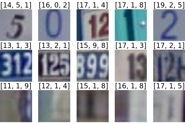
Figure 9: A selection of training images of SVHN whose $20$ ghost feature vectors have a mean ghost prediction smaller than the hit zone threshold. The three rows represent images with different types of peculiarities. A triplet $[\mathtt{a},\mathtt{b},\mathtt{c}]$ indicates that $\mathtt{a}$ hits have been observed in the ghost class $\mathtt{b}$ whereas the true class is $\mathtt{c}$.

4.3.4 Analysis of CIFAR10

Among the training sets analyzed with the use of ghost feature vectors, CIFAR10 seems to be the most reliable. Indeed, using our network, it appears that the $20$ models all agree on the same ghost class for $10728$ training images, which represents $21\%$ of the training images. However, among them, only $15$ have a mean ghost prediction smaller than $0.1$, and a manual check showed that these images are correctly labeled. Most of them $(11)$ are birds or boats whose ghost feature vectors correspond to the airplane class, which is presumably due to their common blue background. We also extended the threshold and checked dozens of images with a mean ghost prediction smaller than $0.2$ (there are $1812$ of them) but we did not find any clearly mislabeled images. Among the images with several ghost classes, those with the most significant predictions did not appear controversial either. Our tests, with the limitations of the architecture of our network, tend to indicate that the dataset is correctly annotated. For the record, using ghost feature vectors in the same way but with a DenseNet-40-12 [6] backbone network before the HoM layer does not reveal misleading images either. It even appears that the $20$ models do not agree on a single ghost class for any image, which tends to confirm that CIFAR10 is a reliable dataset.

5 Conclusion

We introduce the notion of “ghost”, which allows the network to select an alternative choice to the label provided in a classification task without being penalized during the training phase and thus helps detecting abnormalities in training images. This is done by zeroing out the loss associated with the most likely incorrect prediction, which enables the network to build features in line with the correct label of mislabeled samples. After illustrating the use of the ghost loss in a proof of concept experiment, we use it as a tool for analyzing well-known training sets (MNIST, Fashion-MNIST, SVHN, CIFAR10) and detect possible anomalies therein via the novel concept of “sanity matrix”. As far as MNIST is concerned, a few training images that are clearly mislabeled are detected, as well as pairs of images that are almost identical but have different labels, which indicates that the dataset is globally reliable. Regarding Fashion-MNIST, it appears that a large number of training data is considered misleading in some way by the network, suggesting that some classes could be merged, or that some images could deserve multiple labels or that higher resolution images could be provided to define a better classification problem. In SVHN, we find that several dozens of images are either mislabeled, deserve multiple labels, or do not represent any digit, presumably because of the automatic cropping-based labelling process. The CIFAR10 dataset appears to be the most reliable since no particular anomaly is detected. The ghost loss, in combination with a dedicated neural network, could thus be used in the design of a reliability measure for the images of a training set.

Acknowledgements.

This work was supported by the DeepSport project of the Walloon region (Belgium). A. Cioppa has a grant funded by the FRIA (Belgium).

References

- [1] C. Brodley and M. Friedl. Identifying mislabeled training data. Journal of Artificial Intelligence Research, 11:131–167, August 1999.
- [2] A. Deliège, A. Cioppa, M. Van Droogenbroeck. HitNet: a neural network with capsules embedded in a Hit-or-Miss layer, extended with hybrid data augmentation and ghost capsules. CoRR, abs/1806.06519, 2018.
- [3] J. Deng, W. Dong, R. Socher, L. Li, K. Li, and L. Fei-Fei. ImageNet: A large-scale hierarchical image database. In IEEE International Conference on Computer Vision and Pattern Recognition (CVPR), pages 248–255, Miami, Florida, USA, June 2009.
- [4] B. Frenay and M. Verleysen. Classification in the presence of label noise: A survey. IEEE Transactions on Neural Networks and Learning Systems, 25(5):845–869, May 2014.
- [5] Google Creative Lab. Quick, draw! https://quickdraw.withgoogle.com/data, 2017.
- [6] G. Huang, Z. Liu, L. van der Maaten, and K. Weinberger. Densely connected convolutional networks. In IEEE International Conference on Computer Vision and Pattern Recognition (CVPR), pages 2261–2269, Honolulu, Hawaii, USA, July 2017.
- [7] D. Karimi, H. Dou, S. K. Warfield, A. Gholipour. Deep learning with noisy labels: exploring techniques and remedies in medical image analysis CoRR, abs/1912.02911 (v2), 2020.
- [8] A. Krizhevsky. Learning multiple layers of features from tiny images, 2009. Technical report, University of Toronto.
- [9] Y. Lecun, L. Bottou, Y. Bengio, and P. Haffner. Gradient-based learning applied to document recognition. Proceedings of IEEE, 86(11):2278–2324, November 1998.
- [10] H. Lee, J. Lee, S. Kim, E. Yang, and S. Hwang. DropMax: Adaptive variational softmax. CoRR, abs/1712.07834, December 2017.
- [11] G. Mayraz and G. E. Hinton. Recognizing handwritten digits using hierarchical products of experts. IEEE Transactions on Pattern Analysis and Machine Intelligence, 24(2):189–197, February 2002.
- [12] Y. Netzer, T. Wang, A. Coates, A. Bissacco, B. Wu, and A. Ng. Reading digits in natural images with unsupervised feature learning. In Advances in Neural Information Processing Systems (NIPS), volume 2011, Granada, Spain, December 2011.
- [13] G. Patrini, A. Rozza, A. Menon, R. Nock, and L. Qu. Making deep neural networks robust to label noise: A loss correction approach. In IEEE International Conference on Computer Vision and Pattern Recognition (CVPR), pages 2233–2241, Honolulu, Hawaii, USA, July 2017.
- [14] S. Sabour, N. Frosst, and G. Hinton. Dynamic routing between capsules. CoRR, abs/1710.09829, October 2017.
- [15] N. Srivastava, G. Hinton, A. Krizhevsky, I. Sutskever, and R. Salakhutdinov. Dropout: A simple way to prevent neural networks from overfitting. Journal of Machine Learning Research, 15(1):1929–1958, January 2014.
- [16] H. Xiao, K. Rasul, and R. Vollgraf. Fashion-MNIST: a novel image dataset for benchmarking machine learning algorithms. CoRR, abs/1708.07747, 2017.
- [17] Z. Zhang, M. Sabuncu. Generalized cross entropy loss for training deep neural networks with noisy labels. In Advances in Neural Information Processing Systems (NIPS), pages 8778-8788, 2018.
- [18] S. Thulasidasan, T. Bhattacharya, J. Bilmes, G. Chennupati, J. Mohd-Yusof. Combating Label Noise in Deep Learning Using Abstention. In International Conference on Machine Learning (ICML), 2019.
- [19] A. Rusiecki. Trimmed robust loss function for training deep neural networks with label noise. In International Conference on Artificial Intelligence and Soft Computing, 2019.
- [20] J. Speth, E. M. Hand. Automated label noise identification for facial attribute recognition. In IEEE International Conference on Computer Vision and Pattern Recognition Workshops (CVPRW), 2019.
- [21] X. Wang, Y. Hua, E. Kodirov, and N.= M. Robertson. Emphasis Regularisation by Gradient Rescaling for Training Deep Neural Networks with Noisy Labels. CoRR, abs/1905.11233, 2019.
- [22] K.-H. Lee, X. He, L. Zhang, and L. Yang. CleanNet: Transfer Learning for Scalable Image Classifier Training with Label Noise. In IEEE International Conference on Computer Vision and Pattern Recognition (CVPR), pages 5447–5456, Salt Lake City, Utah, USA, June 2018.