A mixed method for 3D nonlinear elasticity using finite element exterior calculus

Abstract

This article discusses a mixed finite element technique for 3D nonlinear elasticity using a Hu-Washizu (HW) type variational principle. In this method, the deformed configuration and sections from its cotangent bundle are the input arguments. The critical points of the proposed HW functional enforce compatibility of these sections with the configuration, in addition to mechanical equilibrium and constitutive relations. This finite element (FE) approximation distinguishes a vector from a 1-from, a feature not commonly found in mixed FE approximations for nonlinear elasticity. This point of view permits us to construct finite elements with vastly superior performance. Discrete approximations for the differential forms appearing in the variational principle are constructed with ideas borrowed from finite element exterior calculus. These are in turn used to construct a discrete approximation to our HW functional. The discrete equations describing mechanical equilibrium, compatibility and constitutive rule, are obtained by extemizing the discrete functional with respect to appropriate degrees of freedom. The discrete extremization problem is then solved using a numerical search technique; we use Newton’s method for this purpose. This mixed FE technique is then applied to a few benchmark problems wherein conventional displacement based approximations encounter locking and checker boarding. These studies help establish that our mixed FE approximation, which requires no artificial stabilising terms, is free of these numerical bottlenecks.

Keywords: Hu-Washizu principle; differential forms; non-linear elasticity; finite element exterior calculus

1 Introduction

Constructing well performing numerical discretization schemes for non-linear elasticity is a challenging research area, having attracted enormous attention over the years because of their usefulness in engineering design and simulation. Earlier efforts in this area were mostly to develop finite element (FE) techniques to approximate the deformation field alone. However, it was soon realised that such approximations were plagued with instabilities such as shear locking, volumetric locking and checker boarding. Techniques based on reduced integration, enhanced and assumed strain techniques [29, 28] were introduced to circumvent these difficulties. Assumed and enhanced strain techniques introduce additional stabilization terms in the variational formulation, the motivation for which is purely numerical. From the literature, it may be gathered that constructing numerical approximations for 3-dimensional non-linear elasticity that takes only the elasticity parameters and works well for quite a broad range of material models, loading and applied constraints is still work in progress. This article is an attempt, perhaps a first of its kind, to address this problem by adopting tools from geometry. Often in mechanics, the distinction between a vector and a 1-form is understated. This blurs the geometric meaning bought about by these ’vectors’. For example, in particle dynamics, both force and velocity may be represented as vectors, even though this representation is physically incorrect; it prevents us from talking about the existence of a potential for a force. If force were to be represented as a 1-form, one could talk about its integrability in the sense of Poincaré, leading to the possible existence of a potential for the force. Moreover, the natural action of a force (a 1-form) on velocity (a vector) yields power without the need for an inner-product. Considering force as a 1-form is common in geometric mechanics [20] and electrodynamics [15]. However, such a description is rare in elasticity and, in general, continuum mechanics of solids.

In an effort to mimic the force-velocity pairing in particle dynamics, Frankel [14] gave a differential form based description of Cauchy and Piola stresses (See Appendix A in [14]). His idea was to decompose stress into area and force components, where the area component was represented by a 2-form and the force component by a 1-form. He also suggested the use of Cartan’s moving frame to describe the equation of non-linear elasticity in arbitrary curvilinear coordinates. However this suggestion went mostly unnoticed. Kanso et al. also gave a description of stress tensor using bundle valued differential forms, their description being very similar to that of Frankel. Building on the work of Frankel and Kanso et al., Dhas and Roy [13] have presented a Hu-Washizu (HW) type mixed variational principle for nonlinear elasticity, which can accommodate a geometric description of deformation and stresses. An important feature of this formulation is its accommodation of the frame fields as an additional input argument making it suitable for problems in which the affine connection evolves, an example being Kirchhoff type shells.

For a deformable solid, the HW functional takes variables from the base space (configuration) and fibre (tangent/ cotangent space) of the deformed configurations tangent bundle as independent. The HW principle then ties these variables together with conditions which establish compatibility between the base space and the fibre to form a tangent bundle. These conditions often reflect certain integrability issues, whose origin can be traced to the geometric hypothesis placed on the configuration of the body. The simplest form of the HW variational principle is the one that takes the Jacobian of deformation as input to the functional [30]. This well known mixed formulation enforces the compatibility between the Jacobian computed from deformation and the independent Jacobian field by introducing pressure as a Lagrange multiplier. Geometrically, the Jacobian of deformation is a volume-form; the compatibility of these volume-forms require them to be equal. In the literature, numerical techniques based on these formulations are often referred to as $p-\Theta$. It is also well understood that constructing a numerical technique by arbitrary interpolations of $p$ and $\Theta$ leads to instability. This example highlights the need for a numerical method that respects the geometric structure imposed on the fields.

Constructing finite dimensional approximations to fields that respect the geometric structure placed on them has a long history. H Whitney [33] discussed a family of finite dimensional approximations for differential forms on a simplicial manifold. In the modern parlance, such approximations correspond to the lowest order FE scheme for differential forms. These FE spaces were developed much before the advent of the finite element method itself. Whitney used these approximations to study the Hodge-Laplacian. This family of finite elements is called the Whitey forms or Whitney elements. The geometric underpinning of this family of finite elements went unnoticed in the literature for quite some time. Recently, these finite elements have come into prominence due to the effort of the computational electromagnetics community [10]. In the finite element literature, the FE spaces constructed by Whitey have been reinvented as the vector finite elements of Raviart-Thomas [24] and Nedelec [21, 22]. The vector finite elements have been developed to approximate mixed variational principles. Arnold and co-workers [3] have however unified these finite elements under the common umbrella of finite element exterior calculus, using the language of differential forms. The last authors interpret these finite elements as polynomial subspaces of differential forms over $\mathbb{R}^{n}$. An introduction to finite element exterior calculus may be found in [4]. Arnold and Logg [6] have presented a classification of finite elements using differential forms; they called this classification the finite element periodic table. It takes into account the geometry of the cell, the degree of the polynomial space and the degree of the differential form. Finite elements featured in the periodic table are complete up to a given polynomial degree. Well known finite elements like Lagrange, Raviart-Thomas, Nedelec, Brezzi-Douglas-Marini (BDM) etc. are all featured in the finite element periodic table alongside the newer ones.

Apart from finite elements for differential forms, numerical approximations based on finite difference techniques that preserve the conservation laws exactly at the discrete level have been developed by Hyman and Shashkov [17]; see [11] for an analysis of these techniques. In the literature, these methods are now called mimetic techniques. Similar efforts have been made by Hirani [16], who discusses a discrete version of exterior calculus on a simplicial mesh. In a discrete setting, Smale [31] has studied electrical circuits using ideas from algebraic topology. Yavari [34] has presented a discretization for elasticity using discrete exterior calculus. A numerical implementation of these ideas for the equations of incompressible linearised elasticity may be found in Angoshtari and Yavari [2]. Schrodër et al. [26] have presented a mixed finite element technique by independently approximating deformation gradient, its cofactor and its determinant along with the displacement field. The motivation for considering the above variables as independent derives from the observation that these quantities relate infinitesimal line, area and volume elements between the reference and deformed configurations. Being mutually dependent, their dependencies are resolved by introducing additional kinetic variables, which enforce the compatibility. The last authors have combined the kinematic and kinetic variables using a HW type functional, which has all the above kinematic and kinetic quantities as arguments. In line with the work of Schrodër et al.[26], Bonet et al. [9] have discussed a formulation for elastic solids under finite deformation using a cross product defined between tensors. They claim that such an approach would lead to simpler expressions for the first and second derivatives of the stored energy function. Based on this algebraic construction, Bonet et al. [8] have discussed a mixed finite element technique for non-linear elastic solids. This mixed finite element technique utilizes the area and volume forms obtained using the cross product definition of tensors as addition kinematic unknowns. Conjugate generalized forces associated with these new kinematic unknowns have been also identified. From the perspective of the present work, the cross product algebra of tensors introduced by Bonet et al. is just a specialization of the exterior algebra used in the study of differentiable manifolds.

In a recent study, Shojaei and Yavari [27] present a mixed finite element technique for non-linear elasticity, based on the HW variational principle. The authors refer to their technique as the ’compatible strain mixed finite element method (CSMFEM)’. In CSMFEM, one independently approximates deformation, deformation gradient and Piola stress. They base their finite element approximation by constructing suitable finite dimensional projection operators for a differential complex describing the equations of non-linear elasticity. The differential complex they use is very similar to the de Rham complex in differential topology. A difficulty with the CSMFEM is the need for a stabilization term which penalises the incompatibility of deformation. Building on the idea of non-linear elasticity complex, Angoshtari and Matin [1] present an FE technique by identifying the approximation spaces for deformation gradient and stress as subspaces of $H(\text{Curl})$ and $H(\text{Div})$ respectively. However, their discrete equilibrium, compatibility and constitutive rules cannot be obtained as critical points of a functional. This implies that the authors are not exploiting an important property of non-linear elasticity which is the existence of a potential. The absence of a variational structure may pose serious difficulties to analyse the approximation technique and place restrictions on the numerical implementation.

In the present work, we build a finite element solution scheme for non-linear elasticity based on a geometric description of the HW variational principle discussed in Dhas and Roy [13]. This finite element technique can be classified as mixed, as it seeks independent approximations for both kinetic and kinematic fields. The principal novelty of our work is that it uses a discretization that respects the geometric information encoded in both stress and strain fields. Instead of treating the right Cauchy-Green deformation tensor as a single geometric object, we think of it as a composite object given by three 1-forms. Such a point of view has the advantage of describing the invariants of the right Cauchy-Green deformation tensor in terms of the exterior product of the 1-forms. Similarly, the first Piola stress may also be understood as a composite object described by the pulled-back area-form and a traction 1-form. Such a description of stress has never been used in computations before.

The rest of the article is organised as follows. Section 2 introduces a geometric approach to the HW variational principle. Instead of taking deformation gradient as the input, we take three 1-forms as input arguments. Retrospectively, three additional 1-forms which represent the force acting on an infinitesimal area are also taken as input. These force 1-forms enforce compatibility between 1-forms representing deformation and the deformation field. In Section 3, we introduce finite element exterior calculus and the finite element spaces $\mathcal{P}_{r}\Lambda^{n}$ and $\mathcal{P}_{r}^{-}\Lambda^{n}$ on a 3-simplex. Using these finite elements, we find a discrete approximation to the HW variational principle introduced in Section 2. Newton’s method is then used to find the extremum of the discrete HW functional. The residue and tangent operators required for Newton’s method is also presented in Section 4. Numerical simulations to validate the finite element approximation is presented in Section 5; problems presented in this section examine the efficiency of our numerical technique against shear locking, volume locking and checker boarding. Finally, Section 6 concludes the article with a brief discussion of the future prospects of the present work.

2 Differential forms and Hu-Washizu variational principle

Our present goal is to describe the HW variational principle using differential forms. The description here will be brief; for complete details on the kinetics and kinematics in terms of differential forms, see [13]. We denote the reference and deformed configurations of the body by $\mathcal{B}$ and $\mathcal{S}$ respectively. Both these configurations can be identified with subsets of three dimensional Euclidean space. The placements or position vectors of a material point in the reference and deformed configurations are denoted by $X$ and $x$ respectively. Under a curvilinear coordinate system, coordinates of the respective position vectors are denoted as $(X^{1},...,X^{3})$ and $(x^{1},...,x^{3})$. The deformation map relating the position vectors of a material point in the reference and deformed configurations is denotes by $\varphi$. In a particular coordinate system, we may denote deformation using its components $\varphi^{i}$. At each tangent space of $\mathcal{B}$ and $\mathcal{S}$, we choose a set of orthonormal vectors and denote them as $\{E_{1},...,E_{3}\}$ and $\{e_{1},...,e_{3}\}$ respectively. We refer to these sets as frames for the reference and deformed configuration. The orthogonality noted above is with respect to the metric tensor of the Euclidean space. The algebraic duals associated with the frame fields of the reference and deformed configurations are denoted by $\{E^{1},...,E^{3}\}$ and $\{e^{1},...,e^{3}\}$; these sets are called co-frames of the reference and deformed configurations. These frame and co-frame fields satisfy the duality relation $E^{i}(E_{j})=\delta^{i}_{j}$ and $e^{i}(e_{j})=\delta^{i}_{j}$. Using the frame and co-frame fields, differentials of the position vector in reference and deformed configurations may be written as,

$${\text{d}}X=E_{i}\otimes E^{i};\quad{\text{d}}x=e_{i}\otimes e^{i}.$$ (1)

The deformation gradient denoted by $F$ is obtained by pulling the co-vector part of ${\text{d}}x$ back to the reference configuration, $F=e^{i}\otimes\varphi^{*}(e_{i})$. $\varphi^{*}(.)$ denotes the pull-back map induced by deformation. Since we extensively employ the pull-back of deformed configuration co-frame, we reserve the notation $\theta^{i}:=\varphi^{*}(e^{i})$ and call them deformation 1-forms. In terms of deformation 1-forms, the deformation gradient can be written as,

$$F=e_{i}\otimes\theta^{i}.$$ (2)

The area-forms of the reference and deformed configurations are denoted by $A^{i}$ and $a^{i}$ respectively. Since the dimension of these two configurations is 3, there are three linearly independent area-forms on each. These area-forms are given by,

$$A^{1} =E^{2}\wedge E^{3};\;A^{2}=E^{3}\wedge E^{1};\;A^{3}=E^{1}\wedge E^{2}$$ (3)

$$a^{1} =e^{2}\wedge e^{3};\;a^{2}=e^{3}\wedge e^{1};\;a^{3}=e^{1}\wedge e^{2}.$$ (4)

The symbol $(.\wedge.)$ denotes the wedge product between two differential forms. In addition to the area-forms of the reference configuration, one may also pull-back the area-form of the deformed configuration to the reference configuration, $\textsf{A}^{i}=\varphi^{*}(a^{i})$. These pulled-back area-forms may be written as,

$$\textsf{A}^{1}=\theta^{2}\wedge\theta^{3};\;\textsf{A}^{2}=\theta^{3}\wedge\theta^{1};\;\textsf{A}^{3}=\theta^{1}\wedge\theta^{2}.$$ (5)

Note that, the pulled-back area-forms span the same linear space spanned by $A^{i}$. Volume-forms on the reference and deformed configurations are denoted by $V$ and $v$ respectively. Similar to the area-forms, one may also pull the volume-form of the deformed configuration back to the reference; we denote the pulled-back volume-form by $\textsf{V}=\varphi^{*}(v)$. In terms of deformation 1-forms, V may be written as,

$$\textsf{V}=\theta^{1}\wedge\theta^{2}\wedge\theta^{3}.$$ (6)

In terms of deformation 1-forms and pulled-back area forms, the invariants of the right Cauchy-Green deformation tensor may be written as,

$$I_{1} =\left\langle\theta^{i},\theta^{i}\right\rangle$$ (7)

$$I_{2} =\left\langle\textsf{A}^{i},\textsf{A}^{i}\right\rangle$$ (8)

$$I_{3} ={}_{\star}(\theta^{1}\wedge\theta^{2}\wedge\theta^{3})$$ (9)

In (9), ${}_{\star}(.)$ denotes the Hodge star operator, which defines an isometry between the spaces of $n$ and $m-n$ differential forms. In defining $I_{1}$ and $I_{2}$, we have used the inner-product induced by the Euclidean metric on the spaces of 1- and 2-forms.

2.1 Hu-Washizu variational principle

In its original form, the HW functional for a hyperelastic elastic solid takes the deformation field, deformation gradient and first Piola stress as inputs. However, in keeping with our setting, we adopt a HW type functional whose input arguments are deformation field and differential forms describing deformation and stress. In terms of these variables, the HW functional may be written as,

$$\Pi(\theta^{i},t^{i},\varphi)=\int_{\mathcal{B}}W(\theta^{i}){\text{d}}V-(t^{i}\otimes\mathsf{A}^{i})\dot{\wedge}(e_{j}\otimes(\theta^{j}-{\text{d}}\varphi^{j}))+\int_{\partial\mathcal{B}_{t}}\left\langle t^{\sharp},\varphi\right\rangle$$ (10)

In the above equation, $t^{i}$ denotes the traction 1-form. Instead of working with the conventional definition of stress, we use a geometric approach to stress originally put fourth by Frankel (see Appendix-C of the book) [14] and later explored by Kanso et al. [18]. The idea behind this construction is to decompose the stress tensor into traction and area forms. This construction is also intuitive, in line with the understanding of stress as traction (force) acting on an infinitesimal area. Using this, the first Piola stress may be defined as the partial pull-back of the Cauchy stress, where the pull-back is applied only to the area leg, leaving the traction undisturbed (for more details see [19] and [18]). Thus the first Piola stress is related to the traction 1-from and pulled-back area-from in the following way,

$$P =t^{i}\otimes\varphi^{*}(a^{i})$$

$$=t^{i}\otimes\textsf{A}^{i}.$$ (11)

In (10), $\partial\mathcal{B}_{t}$ denotes the traction boundary on with $t$ is applied and $(.)^{\sharp}$ denotes the sharp operator introduced to make the contraction consistent. In writing the functional given in (10), we have assumed that the response of the body is described by a stored energy density function $W$. Conventionally, $W$ depends on the right Cauchy-Green deformation tensor. In the present work, we assume the stored energy function to be a function of $\theta^{i}$. However, the dependence is only through the invariants of the right Cauchy-Green deformation tensor described in (7), (8) and (9). The symbol $\dot{\wedge}$ used in (10) denotes the bilinear product, whose definition is somewhat similar to the one given in by Kanso et al.[18]. This algebraic operation is useful in writing the work done by the Piola stress on deformation. For differential forms $a,b,c$ and the vector field $v$, we define $\dot{\wedge}$ as $(a\otimes b)\dot{\wedge}(v\otimes c)=a(v)(b\wedge c)$. Our definition of $\dot{\wedge}$ does not rely on the metric tensor. The definition of $\dot{\wedge}$ given by Kanso et al. uses the metric tensor, which implies that work done by stress is dependent on the metric structure placed on the configuration manifold. However, from classical dynamics, it is well known that one can compute power or work without the metric tensor.

Instead of postulating the relationship between these differential forms, we follow a variational route to obtain these relations, which are obtained as the critical points of the HW functional. The critical points of the HW energy functional (10) are thus given as,

$$\delta_{t^{i}}\Pi :\theta^{i}-{\text{d}}\varphi^{i}=0;\quad i=1,...,3$$ (12)

$$\delta_{\theta^{1}}\Pi :\frac{\partial W}{\partial\theta^{1}}-[t^{1}(e_{1}){}_{\star}(\theta^{2}\wedge\theta^{3})+t^{2}(e_{1}){}_{\star}(\theta^{3}\wedge\theta^{1})+t^{3}(e_{1}){}_{\star}(\theta^{2}\wedge\theta^{1})]^{\sharp}=0$$ (13)

$$\delta_{\theta^{2}}\Pi :\frac{\partial W}{\partial\theta^{2}}-[t^{1}(e_{2}){}_{\star}(\theta^{2}\wedge\theta^{3})+t^{2}(e_{2}){}_{\star}((\theta^{3}\wedge\theta^{1})+t^{3}(e_{2}){}_{\star}(\theta^{1}\wedge\theta^{2})]^{\sharp}=0$$ (14)

$$\delta_{\theta^{3}}\Pi :\frac{\partial W}{\partial\theta^{3}}-[t^{1}(e_{3}){}_{\star}(\theta^{2}\wedge\theta^{3})+t^{2}(e_{3}){}_{\star}(\theta^{3}\wedge\theta^{1})+t^{3}(e_{3}){}_{\star}(\theta^{1}\wedge\theta^{2})]^{\sharp}=0$$ (15)

$$\delta_{\varphi^{i}}\Pi :{\text{d}}(t^{j}(e_{k}))\wedge\mathsf{A}^{j}=0;\quad i=1,...,3.$$ (16)

In the above equation, $\delta_{(.)}W$ denotes the Gateaux derivative of $W$ in the direction of an input argument. Eq. (12) describes the compatibility between the deformation 1-forms and deformation, Eqs. (13) (14) and (15) are the constitutive rules relating the deformation 1-forms and traction 1-forms and Eq. (16) describes mechanical equilibrium. For more details on the variational principle and calculation of critical points of the HW functional, the reader may see [13].

3 Finite element approximation of differential forms

In this section, we discuss a finite dimensional approximation for differential forms using finite element spaces; these approximation spaces can be neatly dealt within the classical definition of finite elements provided by Cairlet [12]. Recall that a finite element is a triplet denoted by $(K,\mathcal{P}(K),\Sigma)$, where $K$ denotes a triangulation or a cell approximation of a given domain, $\mathcal{P}(K)$ denotes the space of piecewise polynomials of degree less than or equal to $n$ defined on $K$ and $\Sigma$ denotes the degrees of freedom, whose values are from the dual space of $\mathcal{P}(K)$. By choosing the degrees of freedom, one prescribes how the piecewise polynomial spaces are glued together globally. The choice of degrees of freedom also provides a basis for the finite element space. Lagrange, Raviart-Thomas and Nédelec finite elements are common examples of finite elements that may be discussed using the definition given above. In this work, we use a simplicial approximation for the domain. The finite element spaces are constructed on a reference simplex and then mapped back to the actual simplex using an affine map. Notations used in this section closely follow those developed by Arnold and co-workers [3, 4].

3.1 Spaces $\mathcal{P}_{r}\Lambda^{n}$ and $\mathcal{P}_{r}^{-}\Lambda^{n}$

We denote the space of $m$-variable polynomials of degree $r$ in $\mathbb{R}^{m}$ by $\mathcal{P}_{r}(\mathbb{R}^{m})$. The space of polynomial differential forms with form degree $n$ and polynomial degree $r$ is denoted by $\mathcal{P}_{r}\Lambda^{n}(\mathbb{R}^{m})$. Often we suppress $\mathbb{R}^{m}$ from our notation and simply denote these spaces by $\mathcal{P}_{r}$ and $\mathcal{P}_{r}\Lambda^{n}$ respectively. By a polynomial differential form, we mean the following: for $v_{1},...,v_{n}\in$ $T\mathbb{R}^{m}$,

$$\mathcal{P}_{r}\Lambda^{n}=\{\omega\in\Lambda^{n}(\mathbb{R}^{m})|\omega(v_{1},...,v_{n})\in\mathcal{P}_{r}\}.$$ (17)

In other words, the coefficient functions of $\omega$ are polynomials of degree $r$. The space $\mathcal{P}_{r}$ has dimension $\binom{r+m}{m}$. The space $\mathcal{P}_{r}\Lambda^{n}$ can be constructed as a product of $m-$ variable polynomials and $n-$degree differential forms. From this construction, the dimension of $\mathcal{P}_{r}\Lambda^{n}$ can be computed as $\binom{m+r}{m}\binom{n}{m}$.

We denote the Koszul operator by $\kappa$; the action of $\kappa$ on a differential form $\omega$ is given by,

$$\kappa\omega=\omega(v_{X},v_{1},...,v_{m-1})$$ (18)

where, $v_{X}$ denotes the vector which translates the point $X\in\mathbb{R}^{m}$ to the origin. Note that $\kappa$ decreases the degree of a differential form by one; in other words, the operator $\kappa$ has degree $-1$. It also increases the polynomial degree of $\omega$ by one. It is readily verifiable that the operator $\kappa$ commutes with affine pull-back; if $L:\mathbb{R}^{n}\rightarrow\mathbb{R}^{n}$ is an affine linear map, then $L^{*}\kappa\omega=\kappa L^{*}\omega$.

Another important subspace of polynomial differential forms discussed by Arnold and co-workers is $\mathcal{P}_{r}^{-}\Lambda^{n}$. The dimension of this space is larger than $\mathcal{P}_{r-1}\Lambda^{n}$, but smaller than $\mathcal{P}_{r}\Lambda^{n}$. The space $\mathcal{P}_{r}^{-}\Lambda^{n}$ is defined as,

$$\mathcal{P}_{r}^{-}\Lambda^{n}=\{\omega\in\mathcal{P}_{r}\Lambda^{k}|\kappa\omega\in\mathcal{P}_{r}\Lambda^{n-1}\}.$$ (19)

The dimension of the space $\mathcal{P}_{r}^{-}\Lambda(\mathbb{R}^{m})$ can be computed as $\binom{r+k-1}{k}\binom{m+r}{m-k}$. For differential form of degrees 0 and $m$, we have $\mathcal{P}_{r}^{-}\Lambda^{0}=\mathcal{P}_{r}\Lambda^{0}$ and $\mathcal{P}_{r}^{-}\Lambda^{m}=\mathcal{P}_{r}\Lambda^{m}$. The spaces $\mathcal{P}_{r}\Lambda^{n}$ and $\mathcal{P}_{r}^{-}\Lambda^{n}$ are both affine invariant. When restricted to a simplex of dimension $m$, these spaces contain well known finite element spaces as special cases for the specific choice of polynomial degree and form degree.

3.2 Simplicial approximations for $\mathcal{B}$ and $\mathcal{S}$

An $n$-simplex in $\mathbb{R}^{m}$, $m\geq n$ is the closed convex-hull generated by $n+1$ points (vertices) in $\mathbb{R}^{m}$. We may also refer to an $n-$simplex by a set containing $n+1$ integers indexing the $n+1$ points. A simplicial complex $K$ of dimension $n$ is a collection of $n$ simplicies such that every face of $K$ is also a simplex in $K$ and if two simplices in $K$ intersect, the intersection is also a simplex in $K$. A three dimensional finite element mesh, constructed using tetrahedra is an example of simplicial complex. The simplicial approximation for the reference and deformed configurations are denoted by $K_{\mathcal{B}}$ and $K_{\mathcal{S}}$ respectively. The finite element basis functions are constructed on a reference tetrahedron, which we denote by $T_{R}$. These basis functions are then pulled-back to the actual tetrahedron using an affine map. The barycentric coordinates of $T_{R}$ are denoted by $\lambda^{i}$, $0\leq i\leq 3$. These coordinates satisfy the well known constraint $\sum_{i=0}^{n}\lambda^{i}=1$. Fig. 1 shows the reference tetrahedron and the numbering used to index the $0-$ and $1-$ simplices. Table 3.2 lists the coordinates of the 0-simplex and the vertices that make up the 1-simplices.

Table 1: Sub-simplices of dimension zero and one for a $3-$ simplex(tetrahedron)

Vertex index	coordinate	Edge index	[$v_{1}$,$v_{2}$]
1	(0,0,0)	1	[1,2]
2	(1,0,0)	2	[1,3]
3	(0,1,0)	3	[1,4]
4	(0,0,1)	4	[2,3]
		5	[2,4]
		6	[3,4]

3.3 Orientation of simplices

The idea of orientation is crucial in defining the global degrees of freedom for a finite element differential form. We say that a manifold is orientable if it admits a global volume form. In the present context, we define a simplex to have a positive orientation if the order of the vertices follow the lexicographic order or an even permutation of the lexicographic order. Using this definition, it follows that there are only two orientations possible for a simplex of any dimension. However, the scenario is quite different when one turns to a simplicial complex constructed using simplices. Orientation is a global property; it may turn out that a simplicial complex may not admit an orientation. We refer to such complexes as non-orientable. A triangulation placed on a Möbious strip is an example of a simplicial complex which does not admit an orientation. We exclude these non-orientable simplicial complexes from further discussions. Figure 1 shows the numbering scheme we use for a 3-simplex; an arrow placed along an edge indicates positive orientation.

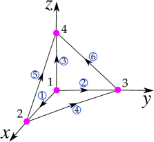
Figure 1: Reference tetrahedron used to construct the basis for the finite element spaces. Edge numbers are marked with circles, while an arrow along an edge indicates a positive orientation.

3.4 Bases for space $\mathcal{P}_{r}\Lambda^{n}(T_{R})$ and $\mathcal{P}_{r}^{-}\Lambda^{n}(T_{R})$

In the previous subsections, we have introduced the simplicial approximation for a configuration and the spaces $\mathcal{P}_{r}\Lambda^{n}$ and $\mathcal{P}_{r}^{-}\Lambda^{n}$. Presently, we discuss finite element basis functions for the spaces $\mathcal{P}_{r}\Lambda^{n}(T_{R})$ and $\mathcal{P}_{r}^{-}\Lambda^{n}(T_{R})$. For differential forms $\omega,\eta\in\Lambda^{n}$, the $L^{2}$ inner product between them is defined as,

$$\left\langle\omega,\eta\right\rangle_{L^{2}}=\int\omega\wedge{}_{*}\eta$$ (20)

The space $L^{2}\Lambda^{n}$ is obtained by completing the space $\Lambda^{n}$ in the norm induced by the inner product $\left\langle.,.\right\rangle_{L^{2}}$. We denote the Hilbert space of differential forms with form degree $n$ by $H\Lambda^{n}$, which is defined as,

$$H\Lambda^{n}=\{\omega\in L^{2}\Lambda^{n}|{\text{d}}\omega\in L^{2}\Lambda^{n+1}\}.$$ (21)

The polynomial spaces $\mathcal{P}_{r}\Lambda^{n}(K)$ and $\mathcal{P}_{r}^{-}\Lambda^{n}(K)$ are constructed by restricting the spaces $\mathcal{P}_{r}\Lambda^{n}(\mathbb{R}^{m})$ and $\mathcal{P}_{r}^{-}\Lambda^{n}(\mathbb{R}^{m})$ to $K$. However, within a finite element framework, the spaces $\mathcal{P}_{r}^{-}{\Lambda}^{n}(K)$ and $\mathcal{P}_{r}{\Lambda}^{n}(K)$ are obtained by gluing together polynomial spaces defined on each simplex $T\in K$. Since we use an affine map to pull the finite element basis from the reference simplex, we need to make sure that the pulled back differential forms are elements in $H\Lambda^{n}$. The following condition is used to enforce this requirement. If $\omega\in H\Lambda^{n}(K)$, $T_{1},T_{2}$ are simplices in $K$ with a common face $f$ of dimension $m-1$, then $\omega|_{f\in T_{1}}=\omega|_{f\in T_{2}}$.

Arnold et al. [5] proposed a geometric decomposition for the dual space of the polynomial spaces $\mathcal{P}_{r}\Lambda^{n}$ and $\mathcal{P}_{r}^{-}\Lambda^{n}$ by mimicking the geometric decomposition for the degrees of freedom for the Lagrange finite element space, leading to the Bernstein basis. For a polynomial differential form with a given degree, they distributed the degrees of freedom on all sub-simplices with dimension greater than or equal to the form degree. This decomposition of the degrees of freedom affords a convenient computational basis index by the sub-simplices. Table 3.4 gives the basis functions for finite element differential forms of degree 0 and 1, in terms of the barycentric coordinates of the 3-simplex.

Table 2: FE basis functions with form degree 0 and 1 and polynomial degree 1

FE spaces	# DoF	Node [i]	Edge $[i,j]$
$\mathcal{P}_{1}\Lambda^{0}(\mathcal{T})$	4	$\lambda^{i}$	-
$\mathcal{P}^{-}_{1}\Lambda^{1}(\mathcal{T})$	6	-	$\lambda^{i}{\text{d}}\lambda^{j}-\lambda^{j}{\text{d}}\lambda^{i}$
$\mathcal{P}_{1}\Lambda^{1}(\mathcal{T})$	12	-	$\lambda^{i}{\text{d}}\lambda^{j},\lambda^{j}{\text{d}}\lambda^{i}$

It should be mentioned that the above basis functions do not take into account the orientation of the simplex; multiplying the basis function by a -1 corrects it for orientation.

4 Discretization of HW variational principle

We now construct a discrete approximation to the HW functional developed in Section 2. To do this we replace the input arguments of the HW functional by their discrete approximation. Given a simplicial approximation for the reference configuration of an elastic body, our objective is to find a simplicial approximation for the deformed configuration, such that the approximation extremizes the discrete HW functional. In addition to this, one also needs to find approximations for the traction and deformation 1-forms. In this work, we use finite element spaces with polynomial degree 1 to approximate deformation and traction 1-forms; displacements are also approximated by polynomials of the same degree. In Section 2, we interpreted traction 1-form as a Lagrange multiplier enforcing the constraint between deformation and deformation 1-forms. This understanding guides us to choose the finite dimensional approximation for traction 1-forms to come from an FE space that is smaller than the FE space for deformation 1-forms. We use the finite element space $\mathcal{P}_{1}\Lambda^{1}$ to interpolate deformation 1-forms and $\mathcal{P}_{1}^{-}\Lambda^{1}$ to approximate traction 1-forms; the dimension of these spaces may be found in 3.4. In our present theory, each displacement component is understood as a zero-form and hence approximated using the FE space $\mathcal{P}_{1}\Lambda^{0}$. Table 4 gives a summary of the FE spaces used to approximate different fields involved in the HW functional. Table 3: Fields and FE spaces used to approximate them Field FE space # Dof Displacement $\mathcal{P}_{1}\Lambda^{0}$ 4 Traction 1-form $\mathcal{P}^{-}_{1}\Lambda^{1}$ 6 Deformation 1-form $\mathcal{P}_{1}\Lambda^{1}$ 12 We introduce the following notations so that the calculations to follow are more readable. The basis functions from the spaces $\mathcal{P}_{1}^{-}\Lambda^{1}$ and $\mathcal{P}_{1}\Lambda^{1}$ are denoted by $\phi^{i}$ and $\psi^{i}$ respectively. Using this new notation, the discrete approximation for different fields involved in the HW functional may be written as,

$$\theta^{i}_{h} :=\sum_{j=1}^{12}\phi^{j}\bar{\theta}_{j}^{i};\quad\phi^{j}\in\mathcal{P}_{1}\Lambda^{1}(T_{\mathcal{B}}),$$ (22)

$$t^{i}_{h} :=\sum_{j=1}^{6}\psi^{j}\bar{t}_{j}^{i};\quad\psi^{j}\in\mathcal{P}_{1}^{-}\Lambda^{1}(T_{\mathcal{B}}),$$ (23)

$$u^{i}_{h} :=\sum_{j=1}^{4}\lambda^{j}\bar{u}^{i}_{j};\quad\lambda^{j}\in\mathcal{P}_{1}\Lambda^{0}(T_{\mathcal{B}}).$$ (24)

In the above equations, the subscript $h$ is introduced to indicate that the right hand side only approximates the actual field. $\bar{\theta}^{i}$, $\bar{t}$ and $\bar{u}^{i}$ denote the degrees of freedom associated with the $i$th deformation and traction 1-form and displacement field respectively. The differential to the displacement approximation can be written as,

$${\text{d}}u^{i}_{h}=\sum_{j=1}^{4}{\text{d}}\lambda^{j}\bar{u}^{i}_{j}.$$ (25)

From Table 4, one may evaluate our present approximation to have 66 DoFs on a 3-simplex. Out of these, 54 are identified with the edges (1 dimensional subsimplices) and the remaining 12 with vertices (0 dimensional subsimplices). In the matrix notation, (22), (23), (24) and (25) may be written as,

$$\theta^{i}_{h}=\boldsymbol{\phi}\boldsymbol{\theta}^{i};\quad t^{i}_{h}=\boldsymbol{\psi}\textbf{t}^{i};\quad u^{i}_{h}=\textbf{N}\textbf{u}^{i};\quad{\text{d}}u^{i}_{h}={\text{d}}\textbf{N}\textbf{u}^{i}.$$ (26)

where, $\boldsymbol{\phi}$, $\boldsymbol{\psi}$, N and dN are matrices with sizes 3 x 12, 3 x 6, 1 x 4 and 3 x 4 respectively. These matrices have the shape functions of the associated FE space as their columns, i.e. $\boldsymbol{\phi}$ has $\phi^{i}$ as its $i$th column and so on. These matrices act on the DoF vector to produce the discrete approximation for the field. The DoF vectors $\boldsymbol{\theta}^{i}$, $\textbf{t}^{i}$ and $\textbf{u}^{i}$ are obtained by stacking the DoFs of the $i$th field one over the other. Using these approximations, the discrete HW functional may be written as,

$$I^{h}=\int_{\mathcal{T}_{\mathcal{B}}}W^{h}{\text{d}}V-(t^{i}_{h}\otimes\textsf{A}^{i}_{h})\dot{\wedge}(e_{j}\otimes(\theta^{j}_{h}-{\text{d}}\varphi^{j}_{h}))+\int_{(\partial\mathcal{T}_{\mathcal{B}})_{t}}\left\langle t^{\sharp},\varphi^{h}\right\rangle.$$ (27)

As usual, we have introduced $h$ as a superscript to indicate that the above functional is only an approximation to the original. Throughout the computations, we assume that the frames $e_{i}$ are fixed and rectilinear.

4.1 Newton’s method

Given a simplicial approximation for the reference configuration of the elastic body, we use Newton’s method to extremize the discrete HW variational functional. The discrete approximation to displacement determines a simplicial approximation for the deformed configuration, while those for deformation and traction 1-forms determine stress and strain states of the body. Newton’s method is a quadratic search technique requiring the first and the second derivatives of the objective functional. In computational mechanics literature, these derivatives are often called residue vector and tangent operator. We now compute the first and second derivatives of the discrete HW functional using the notion of Gateaux derivative. Since we are working in a finite dimensional setting, the Gateaux derivative is much simpler than the one discussed in the previous section. To highlight this difference, we denote the finite dimensional version of the Gateaux derivative by $\textsf{D}_{(.)}I^{h}$. Similarly the second derivatives are denoted by $\textsf{D}_{(.)(.)}I^{h}$, where $(.)$ denotes the DoF vector with respect to which the derivative is calculated. The scheme we use to extremize the discrete HW functional is presented in Algorithm 1. At each Newton iteration, incremental DoFs computed are denoted by prefixing a $\Delta$ before the respecting DoF. These incremental DoFs are obtained by solving the system of linear equations $\mathcal{K}X=-\mathcal{R}$, where $X$ denotes the incremental DoF vector given by, $X=[\Delta\boldsymbol{\theta}^{1},\Delta\boldsymbol{\theta}^{2},\Delta\boldsymbol{\theta}^{3},\Delta\textbf{t}^{1},\Delta\textbf{t}^{2},\Delta\textbf{t}^{3},\Delta\textbf{u}^{1},\Delta\textbf{u}^{2},\Delta\textbf{u}^{3}]^{t}$. The components of the residue vector may be formally written as,

$$\mathcal{R}:=[\textsf{D}_{\boldsymbol{\theta}^{1}}I^{h},\;\textsf{D}_{\boldsymbol{\theta}^{2}}I^{h},\;\textsf{D}_{\boldsymbol{\theta}^{3}}I^{h},\;\textsf{D}_{\textbf{t}^{1}}I^{h},\;\textsf{D}_{\textbf{t}^{2}}I^{h},\;\textsf{D}_{\textbf{t}^{3}}I^{h},\;\textsf{D}_{\textbf{u}^{1}}I^{h},\;\textsf{D}_{\textbf{u}^{2}}I^{h},\;\textsf{D}_{\textbf{u}^{3}}I^{h}]^{t}.$$ (28)

Data:

1. Simplicial approximation for $\mathcal{B}$;

2. Displacement $\textbf{u}^{i}_{prev}$ from the previous load-step;

3. Traction 1-form $\textbf{t}^{i}_{prev}$ from the previous load-step;

4. Deformation 1-form $\boldsymbol{\theta}^{i}_{prev}$ from the previous load-step;

5. Displacement and traction boundary conditions for the current load step;

Result: $\boldsymbol{\theta}^{i},\textbf{t}^{i}$ and $\textbf{u}^{i}$ for the prescribed displacement and traction conditions

Initialize $\mathcal{K}$ as a sparse matrix and $\mathcal{R}$ as a sparse vector;

Initialize $TOL$;

$\textbf{u}^{i}\leftarrow\textbf{u}^{i}_{prev}$;

$\textbf{t}^{i}\leftarrow\textbf{t}^{i}_{prev}$;

$\boldsymbol{\theta}^{i}\leftarrow\boldsymbol{\theta}^{i}_{prev}$;

Modify $\mathcal{R}$ to incorporate traction and displacement conditions;

while $\left\lVert\mathcal{R}\right\rVert\geq TOL$ do

       Initialization: $itEl=1$

      

      while itEl $\leq$ # Elements do

             Compute element $K$ using (38);

             Compute element $R$ using (28);

             Assemble $\mathcal{K}:\mathcal{K}\leftarrow K$;

             Assemble $\mathcal{R}:\mathcal{R}\leftarrow R$;

            

       end while

      Apply displacement boundary conditions to $\mathcal{K}$;

       Solve: $\mathcal{K}X=-\mathcal{R}$;

       $\boldsymbol{\theta}^{i}\leftarrow\boldsymbol{\theta}^{i}+\Delta\boldsymbol{\theta}^{i}$;

       $\textbf{t}^{i}\leftarrow\textbf{t}^{i}+\Delta\textbf{t}^{i}$;

       $\textbf{u}^{i}\leftarrow\boldsymbol{u}^{i}+\Delta\boldsymbol{u}^{i}$;

      

end while

Algorithm 1 Newton’s method for extremising the discrete HW functional

The first derivative of the discrete HW functional with respect to the DoFs associated with the deformation 1-forms can be computed as,

$$\textsf{D}_{\boldsymbol{\theta}^{1}}I^{h} =\int_{\mathcal{T}_{\mathcal{B}}}\textsf{D}_{\boldsymbol{\theta}^{1}}W^{h}-(t^{1}(e_{1})+t^{2}(e_{2})+t^{3}(e_{3}))\boldsymbol{\phi}\wedge\theta^{2}\wedge\theta^{3}$$

$$-t^{2}(e_{1})(\boldsymbol{\phi}\wedge\theta^{3}\wedge{\text{d}}\varphi^{1})-t^{2}(e_{2})(\boldsymbol{\phi}\wedge\theta^{3}\wedge{\text{d}}\varphi^{2})-t^{2}(e_{3})(\boldsymbol{\phi}\wedge\theta^{3}\wedge{\text{d}}\varphi^{3})$$

$$+t^{3}(e_{1})(\boldsymbol{\phi}\wedge\theta^{2}\wedge{\text{d}}\varphi^{1})+t^{3}(e_{2})(\boldsymbol{\phi}\wedge\theta^{2}\wedge{\text{d}}\varphi^{2})+t^{3}(e_{3})(\boldsymbol{\phi}\wedge\theta^{2}\wedge{\text{d}}\varphi^{3}),$$ (29)

$$\textsf{D}_{\boldsymbol{\theta}^{2}}I^{h} =\int_{\mathcal{T}_{\mathcal{B}}}\textsf{D}_{\boldsymbol{\theta}^{2}}W^{h}+(t^{1}(e_{1})+t^{2}(e_{2})+t^{3}(e_{3}))\boldsymbol{\phi}\wedge\theta^{1}\wedge\theta^{3}$$

$$+t^{1}(e_{1})(\boldsymbol{\phi}\wedge\theta^{3}\wedge{\text{d}}\varphi^{1})+t^{1}(e_{2})(\boldsymbol{\phi}\wedge\theta^{3}\wedge{\text{d}}\varphi^{2})+t^{1}(e_{3})(\boldsymbol{\phi}\wedge\theta^{3}\wedge{\text{d}}\varphi^{3})$$

$$-t^{3}(e_{1})(\boldsymbol{\phi}\wedge\theta^{1}\wedge{\text{d}}\varphi^{1})-t^{3}(e_{2})(\boldsymbol{\phi}\wedge\theta^{1}\wedge{\text{d}}\varphi^{2})-t^{3}(e_{3})(\boldsymbol{\phi}\wedge\theta^{1}\wedge{\text{d}}\varphi^{3}),$$ (30)

$$\textsf{D}_{\boldsymbol{\theta}^{3}}I^{h} =\int_{\mathcal{T}_{\mathcal{B}}}\textsf{D}_{\boldsymbol{\theta}^{3}}W^{h}-(t^{1}(e_{1})+t^{2}(e_{2})+t^{3}(e_{3}))\boldsymbol{\phi}\wedge\theta^{1}\wedge\theta^{2}$$

$$-t^{1}(e_{1})(\boldsymbol{\phi}\wedge\theta^{2}\wedge{\text{d}}\varphi^{1})-t^{1}(e_{2})(\boldsymbol{\phi}\wedge\theta^{2}\wedge{\text{d}}\varphi^{2})-t^{1}(e_{3})(\boldsymbol{\phi}\wedge\theta^{2}\wedge{\text{d}}\varphi^{3})$$

$$+t^{2}(e_{1})(\boldsymbol{\phi}\wedge\theta^{1}\wedge{\text{d}}\varphi^{1})+t^{2}(e_{2})(\boldsymbol{\phi}\wedge\theta^{1}\wedge{\text{d}}\varphi^{2})+t^{2}(e_{3})(\boldsymbol{\phi}\wedge\theta^{1}\wedge{\text{d}}\varphi^{3}).$$ (31)

In the above equations, $\boldsymbol{\phi}\wedge\theta^{i}\wedge\theta^{j}:=\sum_{k=1}^{12}\phi^{k}\wedge\theta^{i}\wedge\theta^{j}$. Similarly, $\boldsymbol{\phi}\wedge\theta^{i}\wedge{\text{d}}\varphi^{j}:=\sum_{k=1}^{12}\phi^{k}\wedge\theta^{i}\wedge{\text{d}}\varphi^{j}$. The first derivatives of the discrete HW functional with respect to the DoFs assocaitated with the traction 1-form are given as,

$$\textsf{D}_{\textbf{t}^{1}}I^{h} =\int_{\mathcal{T}_{\mathcal{B}}}-(\boldsymbol{\psi}e_{1})(\theta^{1}\wedge\theta^{2}\wedge\theta^{3})+(\boldsymbol{\psi}e_{1})(\theta^{2}\wedge\theta^{3}\wedge{\text{d}}\varphi^{1})+(\boldsymbol{\psi}e_{2})(\theta^{2}\wedge\theta^{3}\wedge{\text{d}}\varphi^{2})+(\boldsymbol{\psi}e_{3})(\theta^{2}\wedge\theta^{3}\wedge{\text{d}}\varphi^{3}),$$ (32)

$$\textsf{D}_{\textbf{t}^{2}}I^{h} =\int_{\mathcal{T}_{\mathcal{B}}}-(\boldsymbol{\psi}e_{2})(\theta^{1}\wedge\theta^{2}\wedge\theta^{3})+(\boldsymbol{\psi}e_{1})(\theta^{3}\wedge\theta^{1}\wedge{\text{d}}\varphi^{1})+(\boldsymbol{\psi}e_{2})(\theta^{3}\wedge\theta^{1}\wedge{\text{d}}\varphi^{2})+(\boldsymbol{\psi}e_{3})(\theta^{3}\wedge\theta^{1}\wedge{\text{d}}\varphi^{3}),$$ (33)

$$\textsf{D}_{\textbf{t}^{3}}I^{h} =\int_{\mathcal{T}_{\mathcal{B}}}-(\boldsymbol{\psi}e_{3})(\theta^{1}\wedge\theta^{2}\wedge\theta^{3})+(\boldsymbol{\psi}e_{1})(\theta^{1}\wedge\theta^{2}\wedge{\text{d}}\varphi^{1})+(\boldsymbol{\psi}e_{2})(\theta^{1}\wedge\theta^{2}\wedge{\text{d}}\varphi^{2})+(\boldsymbol{\psi}e_{3})(\theta^{1}\wedge\theta^{2}\wedge{\text{d}}\varphi^{3}).$$ (34)

In the above equations, $\boldsymbol{\psi}e_{i}$ is a vector whose components are $\psi^{i}(e_{i})$. The first derivatives of $I^{h}$ with respect to the displacement DoFs may be computed as,

$$\textsf{D}_{\textbf{u}^{1}}I^{h} =\int_{\mathcal{T}_{\mathcal{B}}}t^{1}(e_{1})({\text{d}}\textbf{N}\wedge\theta^{2}\wedge\theta^{3})+t^{2}(e_{1})({\text{d}}\textbf{N}\wedge\theta^{3}\wedge\theta^{1})+t^{3}(e_{1})({\text{d}}\textbf{N}\wedge\theta^{1}\wedge\theta^{2}),$$ (35)

$$\textsf{D}_{\textbf{u}^{2}}I^{h} =\int_{\mathcal{T}_{\mathcal{B}}}t^{1}(e_{2})({\text{d}}\textbf{N}\wedge\theta^{2}\wedge\theta^{3})+t^{2}(e_{2})({\text{d}}\textbf{N}\wedge\theta^{3}\wedge\theta^{1})+t^{3}(e_{2})({\text{d}}\textbf{N}\wedge\theta^{1}\wedge\theta^{2}),$$ (36)

$$\textsf{D}_{\textbf{u}^{3}}I^{h} =\int_{\mathcal{T}_{\mathcal{B}}}t^{1}(e_{3})({\text{d}}\textbf{N}\wedge\theta^{2}\wedge\theta^{3})+t^{2}(e_{3})({\text{d}}\textbf{N}\wedge\theta^{3}\wedge\theta^{1})+t^{3}(e_{3})({\text{d}}\textbf{N}\wedge\theta^{1}\wedge\theta^{2}).$$ (37)

The tangent operator associated with the discrete HW functional may be formally written as,

$$\mathcal{K}=\begin{bmatrix}\textsf{D}_{\boldsymbol{\theta}^{i}}\textsf{D}_{\boldsymbol{\theta}^{j}}I^{h}&\textsf{D}_{\boldsymbol{\theta}^{i}}\textsf{D}_{\textbf{t}^{j}}I^{h}&\textsf{D}_{\boldsymbol{\theta}^{i}}\textsf{D}_{\textbf{u}^{j}}I^{h}\\ &\textsf{D}_{\textbf{t}^{i}}\textsf{D}_{\textbf{t}^{j}}I^{h}&\textsf{D}_{\textbf{t}^{i}}\textsf{D}_{\textbf{u}^{j}}I^{h}\\ \text{Symm}&&\textsf{D}_{\textbf{u}^{i}}\textsf{D}_{\textbf{u}^{j}}I^{h}\end{bmatrix};\quad i,j=1,...,3.$$ (38)

The components of the tangent operator may thus be computed as,

$$\textsf{D}_{\boldsymbol{\theta}^{1}\boldsymbol{\theta}^{1}}I^{h} =\int_{\mathcal{T}_{\mathcal{B}}}\textsf{D}_{\boldsymbol{\theta}^{1}\boldsymbol{\theta}^{1}}W{\text{d}}V;\quad\textsf{D}_{\boldsymbol{\theta}^{2}\boldsymbol{\theta}^{2}}I^{h}=\int_{\mathcal{T}_{\mathcal{B}}}\textsf{D}_{\boldsymbol{\theta}^{2}\boldsymbol{\theta}^{2}}W{\text{d}}V;\quad\textsf{D}_{\boldsymbol{\theta}^{3}\boldsymbol{\theta}^{3}}I^{h}=\int_{\mathcal{T}_{\mathcal{B}}}\textsf{D}_{\boldsymbol{\theta}^{3}\boldsymbol{\theta}^{3}}W{\text{d}}V$$ (39)

$$\textsf{D}_{\boldsymbol{\theta}^{1}\boldsymbol{\theta}^{2}}I^{h} =\int_{\mathcal{T}_{\mathcal{B}}}\textsf{D}_{\boldsymbol{\theta}^{1}\boldsymbol{\theta}^{2}}W{\text{d}}V+(t^{1}(e_{1})+t^{2}(e_{2})+t^{3}(e_{3}))(\boldsymbol{\phi}\wedge\boldsymbol{\phi}\wedge\theta^{3})$$

$$-t^{3}(e_{1})(\boldsymbol{\phi}\wedge\boldsymbol{\phi}\wedge{\text{d}}\varphi^{1})-t^{3}(e_{2})(\boldsymbol{\phi}\wedge\boldsymbol{\phi}\wedge{\text{d}}\varphi^{2})-t^{3}(e_{3})(\boldsymbol{\phi}\wedge\boldsymbol{\phi}\wedge{\text{d}}\varphi^{3})$$ (40)

$$\textsf{D}_{\boldsymbol{\theta}^{1}\boldsymbol{\theta}^{3}}I^{h} =\int_{\mathcal{T}_{\mathcal{B}}}\textsf{D}_{\boldsymbol{\theta}^{1}\boldsymbol{\theta}^{3}}W{\text{d}}V+(t^{1}(e_{1})+t^{2}(e_{2})+t^{3}(e_{3}))(\boldsymbol{\phi}\wedge\boldsymbol{\phi}\wedge\theta^{2})$$

$$-t^{2}(e_{1})(\boldsymbol{\phi}\wedge\boldsymbol{\phi}\wedge{\text{d}}\varphi^{1})-t^{2}(e_{2})(\boldsymbol{\phi}\wedge\boldsymbol{\phi}\wedge{\text{d}}\varphi^{2})-t^{2}(e_{3})(\boldsymbol{\phi}\wedge\boldsymbol{\phi}\wedge{\text{d}}\varphi^{3})$$ (41)

$$\textsf{D}_{\boldsymbol{\theta}^{2}\boldsymbol{\theta}^{3}}I^{h} =\int_{\mathcal{T}_{\mathcal{B}}}\textsf{D}_{\boldsymbol{\theta}^{2}\boldsymbol{\theta}^{3}}W{\text{d}}V+(t^{1}(e_{1})+t^{2}(e_{2})+t^{3}(e_{3}))(\boldsymbol{\phi}\wedge\boldsymbol{\phi}\wedge\theta^{1})$$

$$-t^{1}(e_{1})(\boldsymbol{\phi}\wedge\boldsymbol{\phi}\wedge{\text{d}}\varphi^{1})-t^{1}(e_{2})(\boldsymbol{\phi}\wedge\boldsymbol{\phi}\wedge{\text{d}}\varphi^{2})-t^{1}(e_{3})(\boldsymbol{\phi}\wedge\boldsymbol{\phi}\wedge{\text{d}}\varphi^{3})$$ (42)

$$\textsf{D}_{\boldsymbol{\theta}^{1}\textbf{t}^{1}}I^{h} =\int_{\mathcal{T}_{\mathcal{B}}}-\boldsymbol{\psi}e_{1}\otimes\boldsymbol{\phi}\wedge\theta^{2}\wedge\theta^{3};\textsf{D}_{\boldsymbol{\theta}^{2}\textbf{t}^{2}}I^{h}=\int_{\mathcal{T}_{\mathcal{B}}}-\boldsymbol{\psi}e_{2}\otimes\boldsymbol{\phi}\wedge\theta^{3}\wedge\theta^{1};\textsf{D}_{\boldsymbol{\theta}^{3}\textbf{t}^{3}}I^{h}=\int_{\mathcal{T}_{\mathcal{B}}}-\boldsymbol{\psi}e_{3}\otimes\boldsymbol{\phi}\wedge\theta^{1}\wedge\theta^{2}$$ (43)

$$\textsf{D}_{\textbf{t}^{i}\textbf{t}^{j}}I^{h} =0;\quad\textsf{D}_{\textbf{u}^{i}\textbf{u}^{j}}I^{h}=0$$ (44)

$$\textsf{D}_{\textbf{u}^{1}\textbf{t}^{1}}I^{h} =\int_{\mathcal{T}_{\mathcal{B}}}\boldsymbol{\psi}e_{1}\otimes{\text{d}}\textbf{N}\wedge\theta^{2}\wedge\theta^{3};\quad\textsf{D}_{\textbf{u}^{2}\textbf{t}^{1}}I^{h}=\int_{\mathcal{T}_{\mathcal{B}}}\boldsymbol{\psi}e_{2}\otimes{\text{d}}\textbf{N}\wedge\theta^{2}\wedge\theta^{3};\quad\textsf{D}_{\textbf{u}^{3}\textbf{t}^{1}}I^{h}=\int_{\mathcal{T}_{\mathcal{B}}}\boldsymbol{\psi}e_{3}\otimes{\text{d}}\textbf{N}\wedge\theta^{2}\wedge\theta^{3}$$ (45)

$$\textsf{D}_{\textbf{u}^{1}\textbf{t}^{2}}I^{h} =\int_{\mathcal{T}_{\mathcal{B}}}\boldsymbol{\psi}e_{1}\otimes{\text{d}}\textbf{N}\wedge\theta^{3}\wedge\theta^{1};\quad\textsf{D}_{\textbf{u}^{2}\textbf{t}^{2}}I^{h}=\int_{\mathcal{T}_{\mathcal{B}}}\boldsymbol{\psi}e_{2}\otimes{\text{d}}\textbf{N}\wedge\theta^{3}\wedge\theta^{1};\quad\textsf{D}_{\textbf{u}^{3}\textbf{t}^{2}}I^{h}=\int_{\mathcal{T}_{\mathcal{B}}}\boldsymbol{\psi}e_{3}\otimes{\text{d}}\textbf{N}\wedge\theta^{3}\wedge\theta^{1}$$ (46)

$$\textsf{D}_{\textbf{u}^{1}\textbf{t}^{3}}I^{h} =\int_{\mathcal{T}_{\mathcal{B}}}\boldsymbol{\psi}e_{1}\otimes{\text{d}}\textbf{N}\wedge\theta^{1}\wedge\theta^{2};\quad\textsf{D}_{\textbf{u}^{2}\textbf{t}^{3}}I^{h}=\int_{\mathcal{T}_{\mathcal{B}}}\boldsymbol{\psi}e_{2}\otimes{\text{d}}\textbf{N}\wedge\theta^{1}\wedge\theta^{2};\quad\textsf{D}_{\textbf{u}^{3}\textbf{t}^{3}}I^{h}=\int_{\mathcal{T}_{\mathcal{B}}}\boldsymbol{\psi}e_{3}\otimes{\text{d}}\textbf{N}\wedge\theta^{1}\wedge\theta^{2}$$ (47)

$$\textsf{D}_{\boldsymbol{\theta}^{1}\textbf{t}^{2}}I^{h} =\int_{\mathcal{T}_{\mathcal{B}}}-\boldsymbol{\psi}e_{2}\otimes(\boldsymbol{\phi}\wedge\theta^{2}\wedge\theta^{3})-\boldsymbol{\psi}e_{1}\otimes(\boldsymbol{\phi}\wedge\theta^{3}\wedge{\text{d}}\varphi^{1})-\boldsymbol{\psi}e_{2}\otimes(\boldsymbol{\phi}\wedge\theta^{3}\wedge{\text{d}}\varphi^{2})-\boldsymbol{\psi}e_{3}\otimes(\boldsymbol{\phi}\wedge\theta^{3}\wedge{\text{d}}\varphi^{3})$$ (48)

$$\textsf{D}_{\boldsymbol{\theta}^{1}\textbf{t}^{3}}I^{h} =\int_{\mathcal{T}_{\mathcal{B}}}-\boldsymbol{\psi}e_{3}\otimes(\boldsymbol{\phi}\wedge\theta^{2}\wedge\theta^{3})+\boldsymbol{\psi}e_{1}\otimes(\boldsymbol{\phi}\wedge\theta^{2}\wedge{\text{d}}\varphi^{1})+\boldsymbol{\psi}e_{2}\otimes(\boldsymbol{\phi}\wedge\theta^{2}\wedge{\text{d}}\varphi^{2})+\boldsymbol{\psi}e_{3}\otimes(\boldsymbol{\phi}\wedge\theta^{2}\wedge{\text{d}}\varphi^{3})$$ (49)

$$\textsf{D}_{\boldsymbol{\theta}^{2}\textbf{t}^{1}}I^{h} =\int_{\mathcal{T}_{\mathcal{B}}}+\boldsymbol{\psi}e_{1}\otimes(\boldsymbol{\phi}\wedge\theta^{1}\wedge\theta^{3})+\boldsymbol{\psi}e_{1}\otimes(\boldsymbol{\phi}\wedge\theta^{3}\wedge{\text{d}}\varphi^{1})+\boldsymbol{\psi}e_{2}\otimes(\boldsymbol{\phi}\wedge\theta^{3}\wedge{\text{d}}\varphi^{2})+\boldsymbol{\psi}e_{3}\otimes(\boldsymbol{\phi}\wedge\theta^{3}\wedge{\text{d}}\varphi^{3})$$ (50)

$$\textsf{D}_{\boldsymbol{\theta}^{2}\textbf{t}^{3}}I^{h} =\int_{\mathcal{T}_{\mathcal{B}}}-\boldsymbol{\psi}e_{3}\otimes(\boldsymbol{\phi}\wedge\theta^{3}\wedge\theta^{1})-\boldsymbol{\psi}e_{1}\otimes(\boldsymbol{\phi}\wedge\theta^{1}\wedge{\text{d}}\varphi^{1})-\boldsymbol{\psi}e_{2}\otimes(\boldsymbol{\phi}\wedge\theta^{1}\wedge{\text{d}}\varphi^{2})-\boldsymbol{\psi}e_{3}\otimes(\boldsymbol{\phi}\wedge\theta^{1}\wedge{\text{d}}\varphi^{3})$$ (51)

$$\textsf{D}_{\boldsymbol{\theta}^{3}\textbf{t}^{1}}I^{h} =\int_{\mathcal{T}_{\mathcal{B}}}-\boldsymbol{\psi}e_{1}\otimes(\boldsymbol{\phi}\wedge\theta^{1}\wedge\theta^{2})-\boldsymbol{\psi}e_{1}\otimes(\boldsymbol{\phi}\wedge\theta^{2}\wedge{\text{d}}\varphi^{1})-\boldsymbol{\psi}e_{2}\otimes(\boldsymbol{\phi}\wedge\theta^{2}\wedge{\text{d}}\varphi^{2})-\boldsymbol{\psi}e_{3}\otimes(\boldsymbol{\phi}\wedge\theta^{2}\wedge{\text{d}}\varphi^{3})$$ (52)

$$\textsf{D}_{\boldsymbol{\theta}^{3}\textbf{t}^{2}}I^{h} =\int_{\mathcal{T}_{\mathcal{B}}}\boldsymbol{\psi}e_{2}\otimes(\boldsymbol{\phi}\wedge\theta^{1}\wedge\theta^{2})+\boldsymbol{\psi}e_{1}\otimes(\boldsymbol{\phi}\wedge\theta^{1}\wedge{\text{d}}\varphi^{1})+\boldsymbol{\psi}e_{2}\otimes(\boldsymbol{\phi}\wedge\theta^{1}\wedge{\text{d}}\varphi^{2})+\boldsymbol{\psi}e_{3}\otimes(\boldsymbol{\phi}\wedge\theta^{1}\wedge{\text{d}}\varphi^{3})$$ (53)

$$\textsf{D}_{\boldsymbol{\theta}^{1}\boldsymbol{u}^{1}}I^{h} =\int_{\mathcal{T}_{\mathcal{B}}}-t^{2}(e_{1})({\text{d}}\textbf{N}\wedge\boldsymbol{\phi}\wedge\theta^{3})+t^{3}(e_{1})({\text{d}}\textbf{N}\wedge\boldsymbol{\phi}\wedge\theta^{2})$$ (54)

$$\textsf{D}_{\boldsymbol{\theta}^{1}\boldsymbol{u}^{2}}I^{h} =\int_{\mathcal{T}_{\mathcal{B}}}-t^{2}(e_{2})({\text{d}}\textbf{N}\wedge\boldsymbol{\phi}\wedge\theta^{3})+t^{3}(e_{2})({\text{d}}\textbf{N}\wedge\boldsymbol{\phi}\wedge\theta^{2})$$ (55)

$$\textsf{D}_{\boldsymbol{\theta}^{1}\boldsymbol{u}^{3}}I^{h} =\int_{\mathcal{T}_{\mathcal{B}}}-t^{2}(e_{3})({\text{d}}\textbf{N}\wedge\boldsymbol{\phi}\wedge\theta^{3})+t^{3}(e_{3})({\text{d}}\textbf{N}\wedge\boldsymbol{\phi}\wedge\theta^{2})$$ (56)

$$\textsf{D}_{\boldsymbol{\theta}^{2}\boldsymbol{u}^{1}}I^{h} =\int_{\mathcal{T}_{\mathcal{B}}}+t^{1}(e_{1})({\text{d}}\textbf{N}\wedge\boldsymbol{\phi}\wedge\theta^{3})-t^{3}(e_{1})({\text{d}}\textbf{N}\wedge\boldsymbol{\phi}\wedge\theta^{1})$$ (57)

$$\textsf{D}_{\boldsymbol{\theta}^{2}\boldsymbol{u}^{2}}I^{h} =\int_{\mathcal{T}_{\mathcal{B}}}+t^{1}(e_{2})({\text{d}}\textbf{N}\wedge\boldsymbol{\phi}\wedge\theta^{3})-t^{3}(e_{2})({\text{d}}\textbf{N}\wedge\boldsymbol{\phi}\wedge\theta^{1})$$ (58)

$$\textsf{D}_{\boldsymbol{\theta}^{2}\boldsymbol{u}^{3}}I^{h} =\int_{\mathcal{T}_{\mathcal{B}}}+t^{1}(e_{3})({\text{d}}\textbf{N}\wedge\boldsymbol{\phi}\wedge\theta^{3})-t^{3}(e_{3})({\text{d}}\textbf{N}\wedge\boldsymbol{\phi}\wedge\theta^{1})$$ (59)

$$\textsf{D}_{\boldsymbol{\theta}^{3}\boldsymbol{u}^{1}}I^{h} =\int_{\mathcal{T}_{\mathcal{B}}}+t^{2}(e_{1})({\text{d}}\textbf{N}\wedge\boldsymbol{\phi}\wedge\theta^{1})-t^{1}(e_{1})({\text{d}}\textbf{N}\wedge\boldsymbol{\phi}\wedge\theta^{2})$$ (60)

$$\textsf{D}_{\boldsymbol{\theta}^{3}\boldsymbol{u}^{2}}I^{h} =\int_{\mathcal{T}_{\mathcal{B}}}+t^{2}(e_{2})({\text{d}}\textbf{N}\wedge\boldsymbol{\phi}\wedge\theta^{1})-t^{1}(e_{2})({\text{d}}\textbf{N}\wedge\boldsymbol{\phi}\wedge\theta^{2})$$ (61)

$$\textsf{D}_{\boldsymbol{\theta}^{3}\boldsymbol{u}^{3}}I^{h} =\int_{\mathcal{T}_{\mathcal{B}}}+t^{2}(e_{3})({\text{d}}\textbf{N}\wedge\boldsymbol{\phi}\wedge\theta^{1})-t^{1}(e_{3})({\text{d}}\textbf{N}\wedge\boldsymbol{\phi}\wedge\theta^{2})$$ (62)

5 Numerical study

We now demonstrate the working of the present finite element method through a few benchmark problems in non-linear elasticity. These test problems are carefully designed so as to bring out any pathological behaviour like locking and checker boarding. There are only a few finite element techniques in the literature that can successfully predict the deformation of all the test problems presented in this section. To measure the convergence of the deformation 1-forms, we use the functional norm given by, $\int_{\mathcal{B}}\sum_{i=1}^{3}\left\lVert\theta^{i}\right\rVert^{2}{\text{d}}V$. Similarly the convergence of the first Piola stress is measured using $\int_{\mathcal{B}}\left\lVert P\right\rVert^{2}{\text{d}}V$. Here $P$ is understood as a two tensor by applying a Hodge star on the area leg.

5.1 Cook’s membrane

Cook’s membrane problem is a standard benchmark to test the performance an FE formulation against shear locking. It is now well understood that standard displacement based FE formulations suffer from severe shear locking. Reduced integration and enhanced strain techniques are commonly employed to alleviate this locking, even though these techniques work well under small deformation linear elastic assumptions. Their performance deteriorates in large deformation regimes [7]. We test the performance of our present FE formulation by applying it to Cook’s membrane problem. Our objective here is to study the convergence of the finite element solution for a non-uniform cantilever beam subjected to end shear. The dimensions of the beam, loading arrangement and boundary conditions are is shown in Fig. 2. A maximum load of 100 $N/mm^{2}$ is applied on the loading face, which is reached in 10 loading increments.

Figure 2: Dimensions of the beam, loading arrangement and boundary conditions for Cook’s membrane problem

A Mooney-Rivlin material model with the following stored energy density function is used to describe the stress-strain relation,

$$W=a(I_{1}-3)+b(I_{2}-3)+\frac{c}{2}(J-1)^{2}-d\log(J).$$ (63)

In the numerical simulation, the material parameters $a$, $b$, and $c$ were set as 126, 252, 81661, while the parameter $d$ is given by the relation $d=2a+4b$. These material parameters correspond to a nearly incompressible isotropic elastic material with elastic modulus 2261 and Poisson’s ratio 0.4955 at the reference configuration. The contribution of the stored energy function to the residue vector and tangent operator is thus given by,

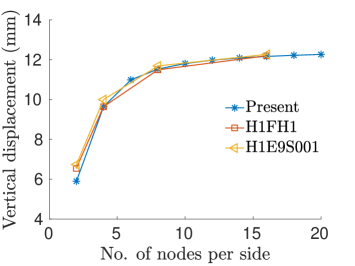
Figure 3: Convergence of tip displacement for Cook’s membrane problem; data for finite elements H1FH1 and H1E9S001 are from Pfefferkorn and Betsch[23]

$$\textsf{D}_{\boldsymbol{\theta}^{i}}W^{h} =a\textsf{D}_{\boldsymbol{\theta}^{i}}I_{1}^{h}+b\textsf{D}_{\boldsymbol{\theta}^{i}}J^{h}+c(J^{h}-1)\textsf{D}_{\boldsymbol{\theta}^{i}}J^{h}-\frac{d}{J^{h}}\textsf{D}_{\boldsymbol{\theta}^{i}}J^{h},$$ (64)

$$\textsf{D}_{\boldsymbol{\theta}^{j}}\textsf{D}_{\boldsymbol{\theta}^{i}}W^{h} =a\textsf{D}_{\boldsymbol{\theta}^{j}}\textsf{D}_{\boldsymbol{\theta}^{i}}I_{1}^{h}+b\textsf{D}_{\boldsymbol{\theta}^{j}}\textsf{D}_{\boldsymbol{\theta}^{i}}I_{2}^{h}+c\textsf{D}_{\boldsymbol{\theta}^{j}}J\otimes\textsf{D}_{\boldsymbol{\theta}^{i}}J^{h}+c(J^{h}-1)\textsf{D}_{\boldsymbol{\theta}^{j}}\textsf{D}_{\boldsymbol{\theta}^{i}}J^{h}$$

$$-d\left[\frac{-1}{J^{h}}\textsf{D}_{\boldsymbol{\theta}^{j}}J^{h}\otimes\textsf{D}_{\boldsymbol{\theta}^{i}}J^{h}+\frac{1}{J^{h}}\textsf{D}_{\boldsymbol{\theta}^{j}}\textsf{D}_{\boldsymbol{\theta}^{i}}J^{h}\right].$$ (65)

The deformed configurations (for 100 $N/mm^{2}$ loading) predicted by our method for different finite element meshes are shown in Fig. 4. To study the convergence of tip displacement, we use a regular mesh with $n+1$ nodes along both $x$ and $y$ directions. Fig. 3 shows the convergence of the tip displacement for different levels of mesh refinement. Our choice of a regular mesh is dictated by the mesh used to generate the convergence plots for the finite elements H1FH1 and H1E9S001, as given in Pfefferkorn and Betsch [23]; these finite elements use a cuboidal mesh to construct the FE spaces. In addition, H1FH1 uses an enhancement for the deformation gradient and H1E9S001 uses an enrichment for the cofactor of the deformation gradient. It should also be emphasised that, for solid mechanics problems, cuboidal finite elements are preferred over simplicial finite elements due to their superior performance for given number of nodes in the FE mesh. Moreover, it may be seen from Fig. 3, our simplicial finite element has comparable performance vis-á-vis the cuboidal finite elements.

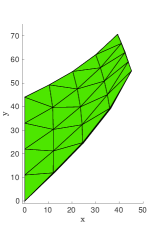
(a) Mesh-1, $n=4$

(b) Mesh-2, $n=8$

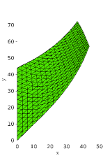
(c) Mesh-3, $n=16$

Figure 4: Deformation of Cook’s membrane predicted by our FE simulation

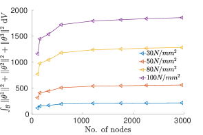
(a) Convergence of deformation 1-forms

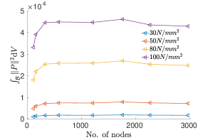
(b) Convergence of first Piola stress

Figure 5: Convergence of deformation 1-forms and first Piola stress for Cook’s membrane problem

The convergence of deformation 1-forms and first Piola stress are shown in Fig. 5. To generate these convergence plots, FE meshes with refinement near the root of the beam were used. Regular meshes with uniform refinement used to study the convergence of displacements required a prohibitively large computational cost to resolve the higher gradients near the root.

5.2 Cube compression

This problem is designed to test the efficiency of the FE approximation against numerical instabilities like hour glassing [25, 27] under extremely large deformation. Conventional displacement based finite elements suffer from such instabilities when subjected to large deformation. In the literature, enhanced strain techniques – again a family of numerical fixes – have been suggested to alleviate such instabilities. We now apply the proposed FE formulation to a cuboid subjected to extremely large compression. The cuboid has a side of length 2 units. To reduce the computational effort, we model only a quarter of the domain. A quarter of the domain along with the loading condition is shown in Fig. 6. This simplification is facilitated by the symmetry of the loading and the boundary conditions. A uniform load is applied on a square region whose side is 1 unit on the top face of the cuboid. This translates to a square of side 0.5 units for the quarter domain. The bottom face of the cuboid is constrained to move vertically, while the loaded region is prevented to move horizontally. A maximum load of $320N/mm^{2}$ was applied in the loaded region, which was reached in multiple load increments. In addition to these, zero displacement boundary conditions are imposed to enforce symmetry of deformation. A Neo-Hookean stored energy function is adopted to represent the stress-strain behaviour of the block. The stored energy function of the material model is given by,

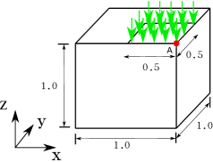
Figure 6: Quarter model of an elastic cube under compression

$$W=\frac{\mu}{2}(I_{1}-3)-\frac{\mu}{2}\log(J)+\frac{\kappa}{8}\log(J)^{2}.$$ (66)

In the numerical simulation, the material parameters $\lambda$ and $\mu$ were set as 400889.806 and 80.194 respectively. These material constants correspond to an isotropic quasi-incompressible material in the reference configuration. The first and the second derivatives of the stored energy function with respect to the degrees of freedom associated with deformation 1-forms may be computed as,

$$\textsf{D}_{\boldsymbol{\theta}^{i}}W^{h} =\frac{\mu}{2}\textsf{D}_{\boldsymbol{\theta}^{i}}I_{1}^{h}-\frac{\mu}{2J^{h}}\textsf{D}_{\boldsymbol{\theta}^{i}}J^{h}+\frac{\kappa}{4J^{h}}\log J^{h}\textsf{D}_{\boldsymbol{\theta}^{i}}J^{h},$$ (67)

$$\textsf{D}_{\boldsymbol{\theta}^{i}}\textsf{D}_{\boldsymbol{\theta}^{j}}W^{h} =\frac{\mu}{2}\textsf{D}_{\boldsymbol{\theta}^{i}}\textsf{D}_{\boldsymbol{\theta}^{j}}I_{1}^{h}+\left(\frac{\mu}{2(J^{h})^{2}}+\frac{\kappa}{4(J^{h})^{2}}-\frac{\kappa\log J^{h}}{4(J^{h})^{2}}\right)\textsf{D}_{\boldsymbol{\theta}^{i}}J^{h}\otimes\textsf{D}_{\boldsymbol{\theta}^{j}}J^{h}+\left(-\frac{\mu}{2J^{h}}+\frac{\kappa}{4J^{h}}\right)\textsf{D}_{\boldsymbol{\theta}^{i}}\textsf{D}_{\boldsymbol{\theta}^{j}}J^{h}.$$ (68)

The deformation predicted by our FE formulation for different simplicial meshes is shown in Fig. 7. For a quantitative comparison, we show the convergence of displacement in the $z$ direction at point A in Fig. 8, where the prediction of our FE formulation is plotted along with those by Reese et al. [25] and Shojaei and Yavari [27]. The solution technique adopted by Shojaei and Yavari is a mixed finite element technique with an additional stabilization term which vanishes at the equilibrium point. Reese et al., on the other hand, have used an enhanced strain based stabilisation technique to arrive at their prediction. From the displacement convergence plots, it is seen that our formulation performs comparable to previously mentioned techniques. However, the main advantage of out formulation is that no additional parameters (like stabilisation parameters) other that the material constants are required in the numerical procedure. Convergence plots of deformation 1-forms and the first Piola stress are given in Fig. 9. A near monotonic convergence is observed.

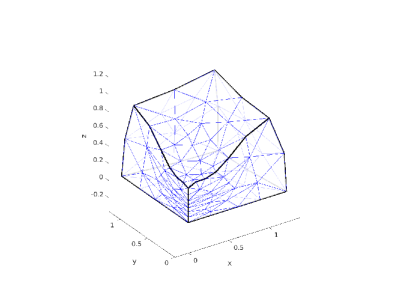
(a) Mesh-1

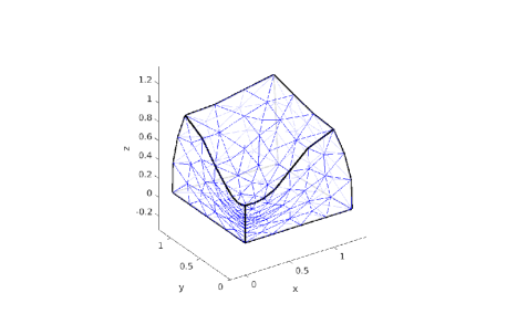
(b) Mesh-2

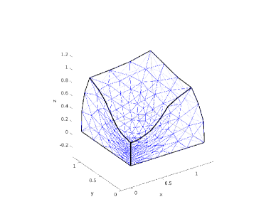
(c) Mesh-3

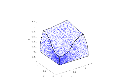
(d) Mesh-4

Figure 7: Deformed shapes of the cube predicted by our FE approximation for different finite element meshes

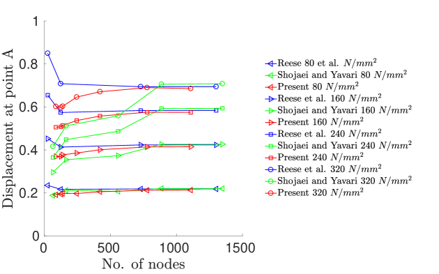
Figure 8: Convergence of displacement at the centre of the loading face

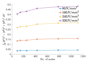
(a) Convergence of deformation 1-forms

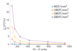
(b) Convergence of Stress

Figure 9: Convergence of deformation 1-form and first Piola stress for the cube compression problem

5.3 Torsion

We now study the effect of extreme mesh distortion during the deformation process. A solid shaft with 1 x 1 cross section and length 10 units is held at one end and subjected to a twist on the other. Fig 10 shows the domain of the problem along with the boundary conditions. The left end of the shaft is constrained in all directions, while on the twisting face all out-of-plane motions are constrained. Instead of applying a twisting moment at the twisting face, displacements are prescribed. In other words, the simulation is performed by rotation control (of the twisting face) and not by a twisting moment. A maximum of 2$\pi$ rotation is applied at the twisting face; this rotation is reached in multiple rotation increments. A compressible isotropic Mooney-Rivilin type material model is used to describe the stress strain relation, whose stored energy function is given by,

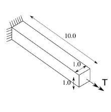
Figure 10: Dimensions, boundary conditions and loading arrangement of a square rod subjected to torsion

$$W=\frac{\alpha}{2}I_{1}^{2}+\frac{\beta}{2}(I_{2})^{2}-\nu\log(J)$$ (69)

The material constants $\alpha$ and $\beta$ were chosen as 24 and 84 respectively and $\nu=(6\alpha+12\beta)$. The contributions of the stored energy function to the residue vector and tangent operator are given by,

$$\textsf{D}_{\boldsymbol{\theta}^{i}}W^{h}= \alpha I_{1}^{h}\textsf{D}_{\boldsymbol{\theta}^{1}}I_{1}^{h}+\beta I_{2}^{h}\textsf{D}_{\boldsymbol{\theta}^{i}}-\frac{\nu}{J^{h}}\textsf{D}_{\boldsymbol{\theta}^{i}}J^{h},$$ (70)

$$\textsf{D}_{\boldsymbol{\theta}^{i}}\textsf{D}_{\boldsymbol{\theta}^{j}}W^{h}= \alpha(\textsf{D}_{\boldsymbol{\theta}^{i}}I_{1}^{h}\otimes\textsf{D}_{\boldsymbol{\theta}^{j}}I_{1}^{h}+I_{1}\textsf{D}_{\boldsymbol{\theta}^{i}}\textsf{D}_{\boldsymbol{\theta}^{j}}I_{1}^{h})+\beta(\textsf{D}_{\boldsymbol{\theta}^{j}}I_{2}^{h}\otimes\textsf{D}_{\boldsymbol{\theta}^{j}}I_{2}^{h}+I_{2}^{h}\textsf{D}_{\boldsymbol{\theta}^{i}}\textsf{D}_{\boldsymbol{\theta}^{j}}I_{1}^{h})$$

$$-\nu\left(-\frac{1}{(J^{h})^{2}}\textsf{D}_{\boldsymbol{\theta}^{i}}J^{h}\otimes\textsf{D}_{\boldsymbol{\theta}^{j}}J^{h}+\frac{1}{J^{h}}\textsf{D}_{\boldsymbol{\theta}^{i}}\textsf{D}_{\boldsymbol{\theta}^{j}}J^{h}\right).$$ (71)

The deformed configurations predicted by our FE procedure for different FE meshes and for a twist angle of $2\pi$ are shown in Fig. 11. The convergence of deformation 1-form and the first Piola stress for different twist angles is shown in Fig. 12.

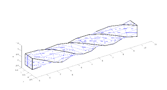
(a) Mesh-1

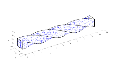
(b) Mesh-2

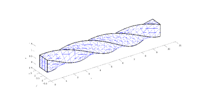
(c) Mesh-3

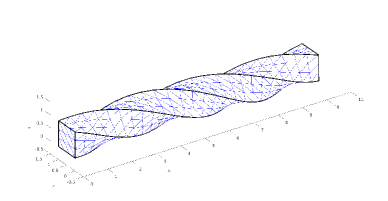
(d) Mesh-4

Figure 11: Deformed shapes of the cube computed using four different finite element meshes

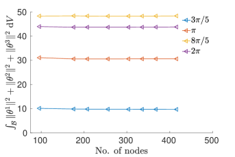
(a) Convergence of deformation 1-form

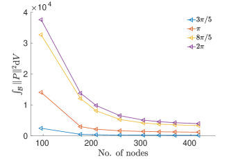
(b) Convergence of traction 1-form

Figure 12: Convergence of deformation and traction 1-forms for the torsion problem

5.4 Shearing of split ring

Finally, we assess the performance of our formulation for a problem where the domain is a little complicated and the deformation is extremely large, even though strains are small (large rotations in some parts of the domain). The domain is an incomplete annulus, obtained by revolving an I shaped cross section to 359 degree about the $y$-axis (the cross section at 0 degree revolution is contained in the $x-z$ plane). The cross section of the annulus at zero degree revolution angle is constrained against all motion. A shear force along the $y$-direction is applied at the centroid of the cross section located at a revolution angle of 359 degree. The cross section and boundary conditions are illustrated in Fig. 13. Wackerfuß and Gruttmann [32] used a rod formulation to study the deformation of this problem. For the geometry and loading conditions, it may be observed that cross sections along the length of the ring undergo a combination of bending, twisting, shearing and extension. In addition, a large segment of the ring undergoes rigid rotation with small strains. A maximum shear force of 12 kN is applied which is reached in multiple loading increments. A Neo-Hookian type material model is used where the stored energy function is given by,

$$W=\frac{\mu}{2}(I_{1}-3)-\mu\ln J+\frac{\lambda}{4}(J^{2}-1-2\ln J)$$ (72)

The material parameters are takes as $\mu=0.4$ and $\lambda=4\alpha$. For the assumed stored energy function, contributions to the residue vector and tangent operator are given by,

$$\textsf{D}_{\boldsymbol{\theta}^{i}}W^{h} =\frac{\mu}{2}\textsf{D}_{\boldsymbol{\theta}^{1}}I_{1}-\frac{\mu}{J}\textsf{D}_{\boldsymbol{\theta}^{i}}+\frac{\lambda}{4}(2J^{h}\textsf{D}_{\boldsymbol{\theta}^{i}}J^{h}-\frac{2}{J}\textsf{D}_{\boldsymbol{\theta}^{i}}J^{h})$$ (73)

$$\textsf{D}_{\boldsymbol{\theta}^{i}}\textsf{D}_{\boldsymbol{\theta}^{j}}W^{h} =\frac{\mu}{2}\textsf{D}_{\boldsymbol{\theta}^{i}}\textsf{D}_{\boldsymbol{\theta}^{j}}I^{h}_{1}-\mu\left(-\frac{1}{(J^{h})^{2}}\textsf{D}_{\boldsymbol{\theta}^{i}}J^{h}\otimes\textsf{D}_{\boldsymbol{\theta}^{j}}J^{h}+\frac{1}{J}\textsf{D}_{\boldsymbol{\theta}^{i}}\textsf{D}_{\boldsymbol{\theta}^{j}}J^{h}\right)$$

$$+\frac{\lambda}{4}\left[2\textsf{D}_{\boldsymbol{\theta}^{i}}J^{h}\otimes\textsf{D}_{\theta^{i}}J^{h}+2J^{h}\textsf{D}_{\theta^{i}}\textsf{D}_{\theta^{j}}J^{h}-2\left(-\frac{1}{(J^{h})^{2}}\textsf{D}_{\boldsymbol{\theta}^{i}}J^{h}\otimes\textsf{D}_{\boldsymbol{\theta}^{j}}J^{h}+\frac{1}{J}\textsf{D}_{\boldsymbol{\theta}^{i}}\textsf{D}_{\boldsymbol{\theta}^{j}}J^{h}\right)\right]$$ (74)

The deformed shapes of the ring for loads of 4, 8 and 12 $kN$ are shown in Fig.15 for different finite element meshes. From the deformed shapes, we see that the ring has undergone extremely large deformation, an evidence for the efficacy of our modelling-cum-discretization approach. The convergence plots of deformation 1-forms and first Piola stress are in Fig. 14.

Figure 13: Geometry and loading condition for a split ring under shear

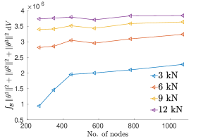
(a) Convergence of deformation 1-forms

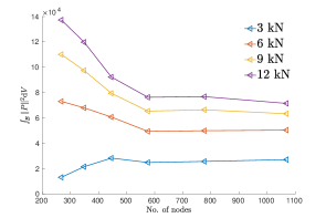
(b) Convergence of traction 1-forms

Figure 14: Convergence of deformation and traction 1-forms for the split ring problem

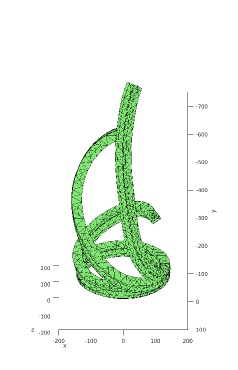
(a) Mesh-2

(b) Mesh-3

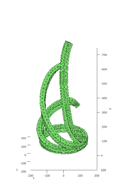
(c) Mesh-3

Figure 15: Deformed shapes of the split ring at different load steps

6 Conclusions

In this article, we have discussed an advanced discretization scheme for non-linear elasticity by bringing together ideas from geometry and finite dimensional approximations of differential forms. The numerical technique is based on a mixed variational principle, whose input arguments are differential forms. We have applied our discretization scheme to certain benchmark problems and, in the process, assessed its performance against shear and volume locking as well as hour-glassing. The numerical study confirms that our FE formulation is free of such numerical difficulties. In the literature, almost all numerical methods which avoid these numerical instabilities use some form of stabilization. The absence of any such stablization term in our variational formulation highlights the superiority of the proposed formulation as well as the discretization technique.

An interesting extension of the present method would be to include inertia in the formulation, wherein schemes based on variational integrators may be used to develop approximations that conserve energy and momenta. An important aspect of Cartan’s moving frame that was not explored in our variational principle is the evolution of the affine connection. For a three dimensional elastic body, such an evolution is redundant since the Euclidean hypothesis on the geometry of the deformed configuration completely fixes it. However, for an elastic shell, the scenario is different. Here the affine connection has to be sought as a solution along with the deformed configuration, when formulated as a mixed problem. We believe that constructing variational principles that take the affine connection as an input is an important direction of future research. These variational principles may then be exploited to build numerical techniques for problems in shell theory and defect mechanics. An equally important research direction is the inclusion of other kinds of interactions like electromagnetism. For the case of electromagnetism, the present formulation is advantageous since electromagnetic fields may also be described as differential forms.

Appendix A Discrete approximation of pulled-back area-forms

The discrete HW principle presented in (27) requires the pulled-back area-forms for their description. Here we present a discretization for the pulled-back area-form in terms of the discrete deformation $1-$ forms given in (22). Formally, the discrete approximation to the pulled-back area forms may be written as,

$$\mathsf{A}^{1}_{h}=\theta^{2}_{h}\wedge\theta^{3}_{h};\quad\mathsf{A}^{2}_{h}=\theta^{3}_{h}\wedge\theta^{1}_{h};\quad\mathsf{A}^{3}_{h}=\theta^{1}_{h}\wedge\theta^{2}_{h}.$$ (75)

The anti-symmetry of the area-forms along with the finite dimensionality of the approximation permits us to find a matrix representation for the discrete area-forms. However, the entries of this matrix are not real numbers but 2-form. Using a finite dimensional approximation (22) for $\theta^{i}$ in (75), we have,

$$\theta^{i}\wedge\theta^{j}=\begin{bmatrix}\bar{\theta}^{i}_{1}\\ \bar{\theta}^{i}_{2}\\ \vdots\\ \bar{\theta}^{i}_{m}\end{bmatrix}^{t}\begin{bmatrix}0&\phi^{1}\wedge\phi^{2}&\ldots&\phi^{1}\wedge\phi^{m}\\ -\phi^{1}\wedge\phi^{2}&0&\ldots&\phi^{2}\wedge\phi^{m}\\ \vdots&\vdots&\ddots&\vdots\\ -\phi^{1}\wedge\phi^{m}&-\phi^{2}\wedge\phi^{m}&\ldots&0\end{bmatrix}\begin{bmatrix}\bar{\theta}^{j}_{1}\\ \bar{\theta}^{j}_{2}\\ \vdots\\ \bar{\theta}^{j}_{m}\end{bmatrix}$$ (76)

The above relationship can be formally written as $\textsf{A}^{k}_{h}=(\boldsymbol{\theta}^{i})^{t}\textbf{W}\boldsymbol{\theta}^{j}$, where the matrix W is skew-symmetric. The matrix W will retain its skew-symmetry as long as the FE spaces used to approximate $\theta^{i}$ and $\theta^{j}$ are the same. The definition of discrete area-form given in (76) can be understood as a discrete wedge operator between two 1-forms. The wedge operator is now given by a skew symmetric matrix W, which depends on the approximation space for $\theta^{i}$. Using the definition of the discrete wedge operator, it is now easy to compute the first derivative of discrete area form which can be written as,

$$\textsf{D}_{\boldsymbol{\theta}^{i}}\mathsf{A}^{k}=\textbf{W}\boldsymbol{\theta}^{j};\quad i\neq j\neq k$$ (77)

Similarly, the second derivative of the area forms can be written as,

$$\textsf{D}_{\boldsymbol{\theta}^{j}\boldsymbol{\theta}^{i}}\mathsf{A}^{k}=\textbf{W};\quad i\neq j\neq k$$ (78)

Appendix B Discrete approximation of stored energy density function

In Section 4, we introduced the discrete approximation to the stored energy function. In the numerical simulations, we assumed that the stored energy function depends on the invariants of the pulled-back metric tensor $C$. We first discretize the invariants of $C$. A discrete approximation to the stored energy function may be constructed by taking the discrete invariants as the input arguments. The discrete stored energy function can thus be written as,

$$W^{h}:=W(I_{1}^{h},I^{h}_{2},J^{h}).$$ (79)

In the above definition, $I_{1}^{h}$, $I_{2}^{h}$ and $J^{h}$ denote the discrete approximations for the invariants of the pulled-back metric tensor.

B.1 Discrete approximation of $I_{1}$ and its derivatives

Using the definition of $I_{1}$ given in (7), its discrete approximation may be written as,

$$I_{1}^{h}:=\sum_{i=1}^{3}\left\langle\theta^{i}_{h},\theta^{i}_{h}\right\rangle$$ (80)

The right hand side of the above definition is a real valued bilinear form. In terms of the shape functions, this bilinear form can be written as,

$$I_{1}^{h}:=\sum_{i=1}^{3}(\boldsymbol{\theta}^{i})^{t}\boldsymbol{\phi}^{t}\boldsymbol{\phi}\boldsymbol{\theta}^{i}$$ (81)

The first derivative of $I_{1}^{h}$ with respect to the DoF vector may now be computed as,

$$\textsf{D}_{\boldsymbol{\theta}^{i}}I_{1}^{h}=2\boldsymbol{\phi}^{t}\boldsymbol{\phi}\boldsymbol{\theta}^{i}$$ (82)

The second derivative with respect to the DoF’s may be evaluated as,

$$\textsf{D}_{\boldsymbol{\theta}^{j}\boldsymbol{\theta}^{i}}I_{1}=\left\{\begin{array}[]{ll}2\boldsymbol{\phi}^{t}\boldsymbol{\phi};&\quad i=j\\ \textbf{0};&\quad i\neq j\end{array}\right.$$ (83)

B.2 Discrete approximation of $I_{2}$ and its derivatives

The discrete approximation of the second invariant of $C$ may be written as,

$$I_{2}^{h}:=\sum_{i=1}^{3}\left\langle\textsf{A}^{i}_{h},\textsf{A}^{i}_{h}\right\rangle$$ (84)

where the discrete approximations for $\textsf{A}^{i}$ are given in (75).

$$\textsf{D}_{\boldsymbol{\theta}^{1}}I_{2}^{h} =-2(\boldsymbol{\phi}\wedge\theta^{3}_{h})\textsf{A}^{2}_{h}+2(\boldsymbol{\phi}\wedge\theta^{2}_{h})\textsf{A}^{3}_{h}$$ (85)

$$\textsf{D}_{\boldsymbol{\theta}^{2}}I_{2}^{h} =2(\boldsymbol{\phi}\wedge\theta^{3}_{h})\textsf{A}^{1}_{h}-2(\boldsymbol{\phi}\wedge\theta^{1}_{h})\textsf{A}^{3}_{h}$$ (86)

$$\textsf{D}_{\boldsymbol{\theta}^{3}}I_{2}^{h} =-2(\boldsymbol{\phi}\wedge\theta^{2}_{h}){\text{d}}\textsf{A}^{1}_{h}+2(\boldsymbol{\phi}\wedge\theta^{1}_{h})\textsf{A}^{2}_{h}$$ (87)

The second derivatives of $I_{2}$ with respect to the DoFs may be computed as,

$$\textsf{D}_{\boldsymbol{\theta}^{1}\boldsymbol{\theta}^{1}}I_{2}^{h} =2(\boldsymbol{\phi}\wedge\theta^{2})^{t}(\boldsymbol{\phi}\wedge\theta^{2})+2(\boldsymbol{\phi}\wedge\theta^{3})^{t}(\boldsymbol{\phi}\wedge\theta^{3})$$ (88)

$$\textsf{D}_{\boldsymbol{\theta}^{2}\boldsymbol{\theta}^{2}}I_{2}^{h} =2(\boldsymbol{\phi}\wedge\theta^{3})^{t}(\boldsymbol{\phi}\wedge\theta^{3})+2(\boldsymbol{\phi}\wedge\theta^{1})^{t}(\boldsymbol{\phi}\wedge\theta^{1})$$ (89)

$$\textsf{D}_{\boldsymbol{\theta}^{3}\boldsymbol{\theta}^{3}}I_{2}^{h} =2(\boldsymbol{\phi}\wedge\theta^{1})^{t}(\boldsymbol{\phi}\wedge\theta^{1})+2(\boldsymbol{\phi}\wedge\theta^{2})^{t}(\boldsymbol{\phi}\wedge\theta^{2})$$ (90)

$$\textsf{D}_{\boldsymbol{\theta}^{1}\boldsymbol{\theta}^{2}}I_{2}^{h} =-2[\boldsymbol{\phi}^{t}(\boldsymbol{\phi}\wedge\textsf{A}^{3})+(\boldsymbol{\phi}\wedge\theta^{1})^{t}(\boldsymbol{\phi}\wedge\theta^{2})]$$ (91)

$$\textsf{D}_{\boldsymbol{\theta}^{2}\boldsymbol{\theta}^{3}}I_{2}^{h} =-2[\boldsymbol{\phi}^{t}(\boldsymbol{\phi}\wedge\textsf{A}^{1})+(\boldsymbol{\phi}\wedge\theta^{2})^{t}(\boldsymbol{\phi}\wedge\theta^{3})]$$ (92)

$$\textsf{D}_{\boldsymbol{\theta}^{3}\boldsymbol{\theta}^{2}}I_{2}^{h} =-2[\boldsymbol{\phi}^{t}(\boldsymbol{\phi}\wedge\textsf{A}^{2})+(\boldsymbol{\phi}\wedge\theta^{3})^{t}(\boldsymbol{\phi}\wedge\theta^{1})]$$ (93)

B.3 Discrete approximation of $J$ and its derivatives

Using the definition of $J$ and FE approximation of deformation 1-forms, the discrete approximation for $J$ can be written as,

$$J^{h}:=\theta^{1}_{h}\wedge\theta^{2}_{h}\wedge\theta^{3}_{h}.$$

The relationship between the deformation 1-form DoFs and $J^{h}$ is trilinear and anti-symmetric. Using the definition of $\theta^{1}_{h}$ in the above expression, we have,

$$J^{h}=(\boldsymbol{\phi}\boldsymbol{\theta}^{1})\wedge(\boldsymbol{\phi}\boldsymbol{\theta}^{2})\wedge(\boldsymbol{\phi}\boldsymbol{\theta}^{3}).$$ (94)

The first derivative can thus be computed as,

$$\textsf{D}_{\theta^{k}}J^{h}=-1^{k+1}\boldsymbol{\phi}\wedge\theta^{i}_{h}\wedge\theta^{j}_{h};\quad i\neq j\neq k;\quad i<j.$$ (95)

Similarly, the second derivative with respect to the DoFs can be computed as,

$$\textsf{D}_{\boldsymbol{\theta}^{1}\boldsymbol{\theta}^{2}}J^{h} =\boldsymbol{\phi}\wedge\boldsymbol{\phi}\wedge\theta^{3}$$

$$\textsf{D}_{\boldsymbol{\theta}^{1}\boldsymbol{\theta}^{3}}J^{h} =-\boldsymbol{\phi}\wedge\boldsymbol{\phi}\wedge\theta^{2}$$ (96)

$$\textsf{D}_{\boldsymbol{\theta}^{2}\boldsymbol{\theta}^{3}}J^{h} =-\boldsymbol{\phi}\wedge\boldsymbol{\phi}\wedge\theta^{1},$$

We also have $\textsf{D}_{\boldsymbol{\theta}^{i}\boldsymbol{\theta}^{i}}J^{h}=\textbf{0}$.

References

- [1] A. Angoshtari and A. G. Matin. A conformal three-field formulation for nonlinear elasticity: From differential complexes to mixed finite element methods. arXiv preprint arXiv:1910.09025, 2019.
- [2] A. Angoshtari and A. Yavari. A geometric structure-preserving discretization scheme for incompressible linearized elasticity. Computer Methods in Applied Mechanics and Engineering, 259:130–153, 2013.
- [3] D. Arnold, R. Falk, and R. Winther. Finite element exterior calculus: from hodge theory to numerical stability. Bulletin of the American mathematical society, 47(2):281–354, 2010.
- [4] D. N. Arnold. Finite Element Exterior Calculus. Society for Industrial and Applied Mathematics, Philadelphia, PA, 2018.
- [5] D. N. Arnold, R. S. Falk, and R. Winther. Geometric decompositions and local bases for spaces of finite element differential forms. Computer Methods in Applied Mechanics and Engineering, 198(21-26):1660–1672, 2009.
- [6] D. N. Arnold and A. Logg. Periodic table of the finite elements. SIAM News, 47(9):212, 2014.
- [7] F. Auricchio, L. B. Da Veiga, C. Lovadina, A. Reali, R. L. Taylor, and P. Wriggers. Approximation of incompressible large deformation elastic problems: some unresolved issues. Computational Mechanics, 52(5):1153–1167, 2013.
- [8] J. Bonet, A. J. Gil, and R. Ortigosa. A computational framework for polyconvex large strain elasticity. Computer Methods in Applied Mechanics and Engineering, 283:1061–1094, 2015.
- [9] J. Bonet, A. J. Gil, and R. Ortigosa. On a tensor cross product based formulation of large strain solid mechanics. International Journal of Solids and Structures, 84:49–63, 2016.
- [10] A. Bossavit. Whitney forms: A class of finite elements for three-dimensional computations in electromagnetism. IEE Proceedings A (Physical Science, Measurement and Instrumentation, Management and Education, Reviews), 135(8):493–500, 1988.
- [11] F. Brezzi, A. Buffa, and G. Manzini. Mimetic scalar products of discrete differential forms. Journal of Computational Physics, 257:1228–1259, 2014.
- [12] P. G. Ciarlet. The finite element method for elliptic problems. SIAM, 2002.
- [13] B. Dhas and D. Roy. A geometric approach to hu-washizu variational principle in nonlinear elasticity. arXiv preprint arXiv:2009.00275, 2020.
- [14] T. Frankel. The geometry of physics: an introduction. Cambridge university press, 2011.
- [15] F. W. Hehl and Y. N. Obukhov. Foundations of classical electrodynamics: Charge, flux, and metric, volume 33. Springer Science & Business Media, 2012.
- [16] A. N. Hirani. Discrete exterior calculus. PhD thesis, California Institute of Technology, 2003.
- [17] J. M. Hyman and M. Shashkov. Adjoint operators for the natural discretizations of the divergence, gradient and curl on logically rectangular grids. Applied Numerical Mathematics, 25(4):413–442, 1997.
- [18] E. Kanso, M. Arroyo, Y. Tong, A. Yavari, J. G. Marsden, and M. Desbrun. On the geometric character of stress in continuum mechanics. Zeitschrift für angewandte Mathematik und Physik, 58(5):843–856, 2007.
- [19] J. E. Marsden and T. J. Hughes. Mathematical foundations of elasticity. Courier Corporation, 1994.
- [20] J. E. Marsden and T. S. Ratiu. Introduction to mechanics and symmetry: a basic exposition of classical mechanical systems, volume 17. Springer Science & Business Media, 2013.
- [21] J.-C. Nédélec. Mixed finite elements in . Numerische Mathematik, 35(3):315–341, 1980.
- [22] J.-C. Nédélec. A new family of mixed finite elements in . Numerische Mathematik, 50(1):57–81, 1986.
- [23] R. Pfefferkorn and P. Betsch. Extension of the enhanced assumed strain method based on the structure of polyconvex strain-energy functions. International Journal for Numerical Methods in Engineering, 121(8):1695–1737, 2020.
- [24] P.-A. Raviart and J.-M. Thomas. A mixed finite element method for 2-nd order elliptic problems. In Mathematical aspects of finite element methods, pages 292–315. Springer, 1977.
- [25] S. Reese, P. Wriggers, and B. Reddy. A new locking-free brick element technique for large deformation problems in elasticity. Computers & Structures, 75(3):291–304, 2000.
- [26] J. Schröder, P. Wriggers, and D. Balzani. A new mixed finite element based on different approximations of the minors of deformation tensors. Computer Methods in Applied Mechanics and Engineering, 200(49-52):3583–3600, 2011.
- [27] M. F. Shojaei and A. Yavari. Compatible-strain mixed finite element methods for 3d compressible and incompressible nonlinear elasticity. Computer Methods in Applied Mechanics and Engineering, 357:112610, 2019.
- [28] J. Simo, F. Armero, and R. Taylor. Improved versions of assumed enhanced strain tri-linear elements for 3d finite deformation problems. Computer methods in applied mechanics and engineering, 110(3-4):359–386, 1993.
- [29] J. C. Simo and M. Rifai. A class of mixed assumed strain methods and the method of incompatible modes. International journal for numerical methods in engineering, 29(8):1595–1638, 1990.
- [30] J. C. Simo and R. L. Taylor. Quasi-incompressible finite elasticity in principal stretches. continuum basis and numerical algorithms. Computer methods in applied mechanics and engineering, 85(3):273–310, 1991.
- [31] S. Smale et al. On the mathematical foundations of electrical circuit theory. Journal of Differential Geometry, 7(1-2):193–210, 1972.
- [32] J. Wackerfuß and F. Gruttmann. A nonlinear hu–washizu variational formulation and related finite-element implementation for spatial beams with arbitrary moderate thick cross-sections. Computer Methods in Applied Mechanics and Engineering, 200(17-20):1671–1690, 2011.
- [33] H. Whitney. Geometric integration theory. Courier Corporation, 2012.
- [34] A. Yavari. On geometric discretization of elasticity. Journal of Mathematical Physics, 49(2):022901, 2008.