A random-supply Mean Field Game price model

Abstract.

We consider a market where a finite number of players trade an asset whose supply is a stochastic process. The price formation problem consists of finding a price process that ensures that when agents act optimally to minimize their trading costs, the market clears, and supply meets demand. This problem arises in market economies, including electricity generation from renewable sources in smart grids. Our model includes noise on the supply side, which is counterbalanced on the consumption side by storing energy or reducing the demand according to a dynamic price process. By solving a constrained minimization problem, we prove that the Lagrange multiplier corresponding to the market-clearing condition defines the solution of the price formation problem. For the linear-quadratic structure, we characterize the price process of a continuum population using optimal control techniques. We include numerical schemes for the price computation in the finite and infinite games, and we illustrate the model using real data.

1. introduction

Mean-field game theory (MFG) is an approach to study the evolution of a population of competitive rational players. Each player solves an optimal control problem that depends on statistical features of the population rather than one-to-one interactions. The statistical features inform the objective of each agent, determining their dynamics. Adopting a MFG approach, the authors in [24] addressed a deterministic price formation model with a market-clearing condition in which the objectives of a continuum of agents are coupled to the price. In this paper, we study a price formation model where $N$ agents interact in a market via the price, $\varpi$, of the commodity they trade and whose supply is random. The agents meet a balance condition that guarantees the supply, $Q$, of the commodity equals its demand. The novelty of our model consists of considering a random supply, such as electricity generation from sustainable sources.

The randomness in price formation has potential applications in renewable energy production on smart grids. Small devices in the grid can store energy that can be sold back to the grid. Changes in weather conditions and network load cause fluctuations in the available supply. Because the agents can sell the surplus of power, they can benefit from load-adaptive pricing ([25], [3]).

To model price formation, there are two different approaches. One approach assumes that the price is a function of the variables in the model. In this setting, [29] compared different pricing policies under partially incomplete, complete, and totally complete information. Their model consisted of a reverse Stackelberg game with non-linear dependence on the price, and price formation is obtained by optimizing the producer’s revenue. The work [14] presented a Cournot model that specified the log-price dynamics, including a Brownian motion and a jump process as common noise. In [3], the spot price is given as a strictly increasing function of the exogenous demand function and the mean energy trading rates. The optimal trading rates were determined by solving a forward-backward system that characterizes the mean-field equilibria. The same authors extended this model in [4] to include penalty terms at random jump times in the state variables. The spot price is an inverse demand function of the expected consumption. They used forward-backward and Riccati equations with jumps to characterize the mean-field equilibrium. The work [2] considered a MFG of optimal stopping to model the switch between traditional and renewable means of energy production. They considered a MFG where the market price couples the agents dynamics, and it is prescribed as a function of a price cap, the exogenous demand, and the supply of both the conventional and the renewable means of production. In their model, the market price is prescribed as a function of a price cap, the exogenous demand, and the supply of both the conventional and the renewable means of production. Recent works have examined the case of intraday electricity markets. [18] studied a linear-quadratic model in the presence of a major player. They distinguished the fundamental price (with no market impact) from the market price. The market price has an explicit form in terms of the average position of the agents, the position of the major agent, and the fundamental price, which is an exogenous variable for the model. The same approach was taken in their consecutive work [19], where the market price depends on the fundamental price and the average position of the agents. They derived a MFG formulation using conditional expectations w.r.t. the common noise and presented a convergence result between the finite model equilibrium to the mean-field model equilibrium as the number of players goes to infinity. They illustrated their results for the EPEX intraday electricity market.

Our work follows a second approach, which was first introduced in [23] and [24]. In this approach, the price is unknown and determined by a balance condition. For instance, [6] proposed a Stackelberg game for revenue-maximization with a linear dependence on the price. The price is obtained using the first-order conditions for the optimization problem. A model for Solar Renewable Energy Certificate Markets (SREC) was presented in [30], where the supply of the energy being priced is controlled. They obtained the SREC price using a market clearing condition and a first-order optimality condition for the optimal planned generation and energy trading. [20] obtained the equilibrium price using a market clearing condition and a forward-backward system of the McKean-Vlasov type characterizing the optimal trading rate for the agents. The same authors studied in [21] a further extension that considers a Major player in the market. The market price is characterized by the solution to a forward-backward stochastic differential equation (SDE) system and a market-clearing condition. In [1], the authors presented a model of $N$ agents with demand forecasts subjected to common noise. In their model, agents meet the demand by selecting controls on their production and trading rate, satisfying an equilibrium condition. The price is obtained using the existence result for a forward-backward coupled system. [16] studied the convergence of a finite-population game to a MFG for a model where traders control their turnover rates with noise in the inventory. They considered a market clearing condition between the aggregated inventory and the supply. The price was obtained by characterizing the Nash equilibrium of the finite-population game using a forward-backward SDE. They illustrated their results using real high-frequency data.

Because the works [30], [20], and [1] deal with a model similar to the one we consider, let us emphasize the novelty in our work. The model in [30] is specialized in the SREC markets, which provides further structure to the model formulation, such as a quadratic cost structure. They used a forward-backward system and variational techniques to formulate a fixed-point problem to prove the existence of a mean-field distribution, from which they get the price. In contrast, we deal with a general convex cost, illustrate our results for the quadratic case, and prove existence using a variational approach. In [20], the authors approximated the equilibrium price by conditioning a stochastic process to the filtration induced by the common noise. They showed that this approximation satisfies the market clearing condition when the number of players increases. In distinction, we obtain a price for which the balance condition for the $N$-players hold. Lastly, [1] derived the price equilibrium using the existence and uniqueness result for a forward-backward coupled system. In contrast, our existence results rely on the calculus of variations approach, whereas we derive forward-backward systems as necessary conditions for such existence. These conditions allow us to identify the price as the Lagrange multiplier for a $N$-agent minimization problem with constraints in which the price is no longer present.

The case of a finite number of players with a deterministic supply was addressed in [5], where only existence and uniqueness were proved, and no numerical approximation scheme was considered. The model we present here generalizes the deterministic supply case. In [22], we addressed the stochastic supply case from the optimal control perspective, and we provided numerical results for a quadratic Lagrangian depending on the trading rate only. The main contribution of this paper is the proof of existence and uniqueness of solutions for the price formation model with a finite number of players in the stochastic case under a general cost function. We adopt a variational approach to obtain our results, and we elaborate on the numerical approximation of solutions.

Next, we introduce our model. Let $T>0$ be the time horizon. In the following, we fix a complete filtered probability space $(\Omega,{\mathcal{F}},\mathds{F},\mathds{P})$; that is, $\mathds{F}=({\mathcal{F}}_{t})_{0\leqslant t\leqslant T}$ is the standard filtration generated by $t\mapsto W_{t}$, a Brownian motion in ${\mathbb{R}}$ (see [28], Definition 3.1.3, and [15], Section 2, for additional details). Here, $W$ plays the role of the common noise in the sense that the supply follows the stochastic differential equation (SDE)

$$dQ_{t}=b^{S}(Q_{t},t)dt+\sigma^{S}(Q_{t},t)dW_{t}.$$ (1.1)

In our model, the agent’s interaction determines the market equilibrium price of the commodity. All of this commodity produced is consumed entirely. Let $N$ be the number of agents and let the state variable $X^{i}_{t}$ account for the quantity of the commodity held by agent $i$ at time $t$. Each agent controls its trading rate according to

$$dX_{t}=v_{t}dt,~{}t\in[0,T],$$ (1.2)

where $v:[0,T]\times\Omega\to{\mathbb{R}}$, the control variable, is progressively measurable with respect to $\mathds{F}$. The optimization problem we consider reads:

Problem 1.

Let $N$ be the number of agents. Let the supply, $Q$, be a stochastic process adapted to $\mathds{F}$ solving (1.1). Let $L\in C^{1}({\mathbb{R}}^{2};{\mathbb{R}})$ be a non-negative Lagrangian, and $\Psi\in C^{1}({\mathbb{R}})$ be a non-negative terminal cost. Assume that at time $t=0$, each agent $i$ owns a quantity $x_{0}^{i}\in{\mathbb{R}}$ of the commodity.

Find a price process $\varpi$ and control processes $v^{i}$, all adapted to $\mathds{F}$, such that for each $i$, with $1\leqslant i\leqslant N$, $X^{i}$ solves (1.2) with the initial condition $X^{i}_{0}=x^{i}_{0}$, and minimizes the cost functional

$${\mathds{E}}\left[\int_{0}^{T}L(X^{i}_{t},v^{i}_{t})+\varpi_{t}v_{t}^{i}~{}dt+\Psi(X^{i}_{T})\right],$$ (1.3)

subject to the balance condition

$$\frac{1}{N}\sum_{i=1}^{N}v_{t}^{i}=Q_{t},\quad\mbox{\emph{ for }}0\leqslant t\leqslant T.$$ (1.4)

The functional (1.3) represents the expected cost for a representative agent on $[0,T]$. This cost consists of three parts: the trading at the current price through the linear term $\varpi v$, the charges related to storage or market impact encoded in $L$, and the terminal cost; the terminal cost reflects the preferences of players at the terminal time. The balance condition (1.4) guarantees demand consumes all supply. For this problem, we obtain the following result:

Theorem 1.1.

Let $Q\in\mathds{H}_{\mathds{F}}$ and suppose that Assumptions 1-5 hold. Then, there exists control processes ${v^{*}}^{i}$, for $1\leqslant i\leqslant N$, and a price process $\varpi$ that solve Problem 1. Furthermore, under Assumption 6, the price $\varpi$ and the control processes ${v^{*}}^{i}$, for $1\leqslant i\leqslant N$, solving Problem 1, are unique.

We prove this theorem in Section 4, where we formulate a problem independent of the price, but the constraint imposed by the balance condition is still present. Existence for this problem is obtained by the direct method in the calculus of variations, and we obtain a forward-backward characterization of optimizers, which allows identifying the price as the Lagrange multiplier corresponding to the balance constraint.

The outline of the paper is as follows: In Section 2, we introduce the main assumptions for the model as well as the notation for the function spaces. In Section 3, we study the optimization problem that a representative agent solves under the assumption that the price is known, which corresponds to the optimization problem that all agents solve simultaneously in the the $N$-agent problem. Using the representative agent result, we prove the existence of a solution to the $N$ agent price formation problem, Problem 1, in Section 4. We specialize our results for a linear-quadratic structure of the model in Section 5. Using optimal control techniques and an extended-state space approach, we obtain semi-explicit expressions for the price with finite $N$ agents and infinite agents. We discuss the convergence as $N\to\infty$ of the former to the latter. The general case is beyond the scope of this paper. The numerical computation of the price is discussed in Section 6, where we present numerical results for a generic model of Section 5 and a calibrated model based on real data from the electricity grid in Spain.

2. Assumptions and notation

We consider natural assumptions in the context of the calculus of variations (see [13]). The following conditions are used to prove the existence of minimizers of (3.2), (4.2), and (4.4). In the following, we suppose the Lagrangian $L$ is non-negative.

Assumption 1.

The Lagrangian $L\in C^{1}({\mathbb{R}}^{2};{\mathbb{R}}^{+}\cup\{0\})$ is convex in $(x,v)$; that is, $(x,v)\mapsto L(x,v)$ is convex.

Assumption 2.

The terminal cost $\Psi\in C^{1}({\mathbb{R}};{\mathbb{R}}^{+}\cup\{0\})$ is convex.

Because we consider integrals w.r.t. measure spaces, we require compositions of processes with functions to remain in the same class where the process is taken. The following growth conditions guarantee this.

Assumption 3.

$\Psi\in C^{1}({\mathbb{R}};{\mathbb{R}}^{+}\cup\{0\})$ satisfies, for some $C>0$,

$$\Psi(x)\leqslant C(1+|x|^{2}),\quad\mbox{for all }x\in{\mathbb{R}}.$$

Moreover, its derivative, which we denote by $\Psi^{\prime}$, satisfies, for some $\tilde{C}>0$,

$$|\Psi^{\prime}(x)|\leqslant\tilde{C}(1+|x|).$$

Assumption 4.

$L\in C^{1}({\mathbb{R}}^{2};{\mathbb{R}}^{+}\cup\{0\})$, and there exists $\tilde{\beta},C>0$ such that

$$L(x,v) \leqslant\tilde{\beta}(1+|v|^{2}),\quad\mbox{ for all }x\in{\mathbb{R}},$$

$$|L_{x}(x,v)|,|L_{v}(x,v)| \leqslant C(1+|v|),\quad\mbox{for all }(x,v)\in{\mathbb{R}}^{2}.$$

In convex optimization, a natural assumption to obtain the existence of minimizers is the coercivity condition.

Assumption 5.

(Coercivity) For some $\alpha>0$ and $\beta\geqslant 0$

$$\alpha|v|^{2}-\beta\leqslant L(x,v),\quad\mbox{ for all }x,v\in{\mathbb{R}}.$$

To guarantee the uniqueness of minimizers, we consider next a strong form of convexity. In turn, this assumption implies the coercivity condition ([7], Corollary 11.17).

Assumption 6.

(Uniform convexity) For some $\theta>0$

$$v\mapsto L(x,v)-\frac{\theta}{2}|v|^{2}\quad\mbox{ is convex for all }x\in{\mathbb{R}}.$$

We introduce the Hamiltonian, $H$, the Legendre transform of $L$, by

$$H(x,p)=\sup_{v\in{\mathbb{R}}}\left\{-pv-L(x,v)\right\}.$$ (2.1)

Recall that when the map $v\mapsto L(x,v)$ is convex, $H(x,p)$ is well defined. Furthermore, if $v\mapsto L(x,v)$ is strictly convex, $L\in C^{2}({\mathbb{R}}^{2};{\mathbb{R}})$, and Assumption 5 holds, there exists a unique value $v^{*}$ where the supremum is attained. In addition,

$$v^{*}=-H_{p}(x,p)~{}\mbox{if and only if}~{}p=-L(x,v^{*}),\mbox{ and hence }H(x,p)=-pv^{*}-L(x,v^{*}).$$ (2.2)

See [11], Theorem A. 2.5, for the proof of the previous results. For the Hamiltonian, we additionally require no more than linear growth of the gradient in the $p$ component, as we state next.

Assumption 7.

The Hamiltonian $H$ satisfies, for some $C>0$,

$$|H_{p}(x,p)|\leqslant C(1+|p|),\quad\mbox{for all }(x,p)\in{\mathbb{R}}^{2}.$$

Now, we set up the notation. Define the space $\mathds{H}_{\mathds{F}}$ as the set of processes $v:[0,T]\times\Omega\to{\mathbb{R}}$, that are measurable and adapted w.r.t. $\mathds{F}$, and satisfy $\|v\|_{\mathds{H}_{\mathds{F}}}^{2}<\infty$, where

$$\langle v,w\rangle_{\mathds{H}_{\mathds{F}}}:={\mathds{E}}\left[\int_{0}^{T}v_{t}w_{t}dt\right],\quad\|v\|_{\mathds{H}_{\mathds{F}}}^{2}:=\langle v,v\rangle_{\mathds{H}_{\mathds{F}}}.$$

This expectation is w.r.t. the measure induced by the Brownian motion. $\mathds{H}_{\mathds{F}}$ is a Hilbert space ([12], Remark 2.2.). Given $v\in\mathds{H}_{\mathds{F}}$, the solution to (1.2) with the initial condition $x_{0}\in{\mathbb{R}}$ is

$$X_{t}=x_{0}+\int_{0}^{t}v_{s}ds.$$

Notice that $X\in\mathds{H}_{\mathds{F}}$ because $\|X\|_{\mathds{H}_{\mathds{F}}}^{2}\leqslant 2T|x_{0}|^{2}+2T^{2}\|v\|_{\mathds{H}_{\mathds{F}}}^{2}$. For our purposes, we consider trajectories with initial condition $x_{0}\in{\mathbb{R}}$.

For $N\in{\mathbb{N}}$, we define $\mathds{H}_{\mathds{F}}^{N}$, where ${\bf v}=(v^{1},\ldots,v^{N})\in\mathds{H}_{\mathds{F}}^{N}$ provided $v^{i}\in\mathds{H}_{\mathds{F}}$, and

$$\langle{\bf v},{\bf w}\rangle_{\mathds{H}_{\mathds{F}}^{N}}:=\sum_{i=1}^{N}\langle v^{i},w^{i}\rangle_{\mathds{H}_{\mathds{F}}},\quad\|{\bf v}\|_{\mathds{H}_{\mathds{F}}^{N}}^{2}:=\sum_{i=1}^{N}\|v^{i}\|_{\mathds{H}_{\mathds{F}}}^{2}.$$

The analysis of Problem 1 relies on the results for the optimization problem faced by a representative agent, which we consider in the next section.

3. The optimization problem for a representative agent

In this section, we assume that a price, $\varpi$, is given. We derive a weak formulation for the Euler-Lagrange equation associated with the optimal control problem for a representative agent. We use this result in Section 4 to study how the collective actions of the agents determine the price.

Let $x_{0}\in{\mathbb{R}}$. Given $v\in\mathds{H}_{\mathds{F}}$, consider the dynamics for the agent

$$\begin{cases}dX_{t}=v_{t}dt,~{}t\in[0,T]\\ X_{0}=x_{0}.\end{cases}$$ (3.1)

Given a price process $\varpi\in\mathds{H}_{\mathds{F}}$, the agent selects $v\in\mathds{H}_{\mathds{F}}$ aiming to reach

$$\inf_{v\in\mathds{H}_{\mathds{F}}}{\mathds{E}}\left[\int_{0}^{T}L(X_{t},v_{t})+\varpi_{t}v_{t}~{}dt+\Psi(X_{T})\right]$$ (3.2)

$$\mbox{subject to }\quad X~{}\mbox{ solves }~{}\eqref{eq: agent dynamics with initial condition}.$$

Let

$$I[v]:={\mathds{E}}\left[\int_{0}^{T}L(X_{t},v_{t})+\varpi_{t}v_{t}~{}dt+\Psi(X_{T})\right],$$

where $X$ solves (3.1) for $v$. In the following, we study the existence and uniqueness of solutions to (3.2). We adopt the direct method of the calculus of variations. Hence, we begin by proving that the functional $I[\cdot]$ is weakly lower semi-continuous.

Proposition 3.1.

Let $x_{0}\in{\mathbb{R}}$ and $\varpi\in\mathds{H}_{\mathds{F}}$. Under Assumptions 1-4, the functional $I[\cdot]$ is weakly lower semi-continuous in $\mathds{H}_{\mathds{F}}$.

Proof.

We will prove that $I[\cdot]$ is convex and lower semi-continuous, from which weak lower semi-continuity follows ([26] Theorem 7.2.5). First, notice that, by Assumptions 1 and 2, $I[\cdot]$ is convex. To prove lower semi-continuity, let $(v^{k})_{k\in{\mathbb{N}}}$ in $\mathds{H}_{\mathds{F}}$ be such that $v^{k}$ converges to $v$. Denote by $X^{k}$ and $X$ the solutions to (3.1) with the controls $v^{k}$ and $v$, respectively. Notice that, because the trajectories $X^{k}$ and $X$ have the same initial condition, we have

$$\|X^{k}-X\|_{\mathds{H}_{\mathds{F}}}^{2}\leqslant 2T^{2}\|v^{k}-v\|_{\mathds{H}_{\mathds{F}}}^{2}.$$

Therefore, $X^{k}$ converges to $X$. The convexity in Assumptions 1 and 2 imply ([7], Proposition 17.7)

$$L_{v}(X_{t},v_{t})(v^{k}_{t}-v_{t})+L(X_{t},v_{t})\leqslant L(X_{t},v^{k}_{t}),$$ (3.3)

$$\Psi^{\prime}(X_{T})(X_{T}^{k}-X_{T})+\Psi(X_{T})\leqslant\Psi(X_{T}^{k}).$$ (3.4)

Adding $L(X^{k}_{t},v^{k}_{t})-L(X_{t},v^{k}_{t})+\varpi_{t}v_{t}$ to both sides of (3.3), we get

$$L_{v}(X_{t},v_{t})(v^{k}_{t}-v_{t})-L(X_{t},v^{k}_{t})+L(X^{k}_{t},v^{k}_{t})+L(X_{t},v_{t})+\varpi_{t}v_{t}$$

$$\leqslant\varpi_{t}(v_{t}-v^{k}_{t})+L(X^{k}_{t},v^{k}_{t})+\varpi_{t}v^{k}_{t}.$$

Taking ${\mathds{E}}[\int_{0}^{T}\cdot~{}dt]$ in the previous inequality, ${\mathds{E}}[\cdot]$ in (3.4), and adding both results, we obtain

$$\langle L_{v}(X,v),v^{k}-v\rangle_{\mathds{H}_{\mathds{F}}}+{\mathds{E}}\left[\int_{0}^{T}L(X^{k}_{t},v^{k}_{t})-L(X_{t},v^{k}_{t})~{}dt\right]+I[v]+{\mathds{E}}\left[\Psi^{\prime}(X_{T})(X^{k}_{T}-X_{T})\right]$$

$$\leqslant\langle\varpi,v-v^{k}\rangle_{\mathds{H}_{\mathds{F}}}+I[v^{k}].$$ (3.5)

By Assumption 4, $L_{v}(X,v)\in\mathds{H}_{\mathds{F}}$, hence

$$\langle L_{v}(X,v),v^{k}-v\rangle_{\mathds{H}_{\mathds{F}}}\to 0.$$ (3.6)

By Assumption 3, $\Psi^{\prime}(X_{T})\in\mathds{H}_{\mathds{F}}$, and using the representation $X_{T}^{k}-X_{T}=\int_{0}^{T}v^{k}_{t}-v_{t}~{}dt$, we obtain

$${\mathds{E}}[\Psi^{\prime}(X_{T})(X^{k}_{T}-X_{T})]\to 0.$$ (3.7)

By Assumption 4, the Cauchy inequality, and the triangle inequality

$$\left|{\mathds{E}}\left[\int_{0}^{T}L(X^{k}_{t},v^{k}_{t})-L(X_{t},v^{k}_{t})~{}dt\right]\right| \leqslant C\langle|X^{k}-X|,1+|v^{k}|\rangle_{\mathds{H}_{\mathds{F}}}-$$

$$\leqslant C\|X^{k}-X\|_{\mathds{H}_{\mathds{F}}}\left(T+\|v^{k}\|_{\mathds{H}_{\mathds{F}}}\right)\to 0.$$

Using the previous inequality, (3.6), (3.7), and the assumption on $\varpi$, taking $\liminf$ in (3), we obtain

$$I[v]\leqslant\liminf_{k\in{\mathbb{N}}}I[v^{k}].$$

Therefore, $I[\cdot]$ is lower semi-continuous. ∎

Proposition 3.2.

Suppose that Assumptions 1- 5 hold. Given an initial condition $x_{0}\in{\mathbb{R}}$ and a price process $\varpi\in\mathds{H}_{\mathds{F}}$, there exists an optimal control $v^{*}\in\mathds{H}_{\mathds{F}}$ that solves (3.2). Furthermore, under Assumption 6, $v^{*}$ is unique.

Proof.

To prove existence, we use the direct method in the calculus of variations. By Assumption 5, we have

$$\alpha\left(v+\frac{\varpi}{2\alpha}\right)^{2}-\frac{\varpi^{2}}{4\alpha}-\beta\leqslant L(x,v)+v\varpi.$$ (3.8)

Since $\varpi\in\mathds{H}_{\mathds{F}}$, select $a$ and $b$ such that

$$0<a<\alpha,\quad\tfrac{1}{2(\alpha-a)}\|\varpi\|_{\mathds{H}_{\mathds{F}}}^{2}\leqslant b.$$

Then, for any $v\in\mathds{H}_{\mathds{F}}$, we have

$$0\leqslant(\alpha-a){\mathds{E}}\left[\int_{0}^{T}\left(v_{t}+\tfrac{1}{2(\alpha-a)}\varpi_{t}\right)^{2}dt\right]+b-\tfrac{1}{2(\alpha-a)}\|\varpi\|_{\mathds{H}_{\mathds{F}}}^{2}.$$

The previous inequality, (3.8), and $0\leqslant\Psi$ in Assumption 2, imply

$$a\|v\|_{\mathds{H}_{\mathds{F}}}^{2}-b-\beta T\leqslant{\mathds{E}}\left[\int_{0}^{T}\alpha(v_{t})^{2}+\varpi_{t}v_{t}-\beta~{}dt\right]\leqslant I[v]$$

for all $v\in\mathds{H}_{\mathds{F}}$. Therefore, $v\mapsto I[v]$ is coercive, and in particular, the infimum in (3.2) is finite. Let $(v^{k})_{k\in{\mathbb{N}}}$ in $\mathds{H}_{\mathds{F}}$ be a minimizing sequence; that is,

$$\lim_{k\to+\infty}I[v^{k}]=\inf_{v\in\mathds{H}_{\mathds{F}}}I[v].$$

By the coercivity of $I[\cdot]$, $(v^{k})_{k\in{\mathbb{N}}}$ is bounded in $\mathds{H}_{\mathds{F}}$. Recall that $\mathds{H}_{\mathds{F}}$ is a Hilbert space, so it is reflexive and, therefore, weakly precompact ([17], Appendix D, Theorem 3). Hence, there exists a subsequence, still denoted by $v^{k}$, that weakly converges to $v^{*}\in\mathds{H}_{\mathds{F}}$; that is, for all $w\in\mathds{H}_{\mathds{F}}$

$$\langle v^{k},w\rangle_{\mathds{H}_{\mathds{F}}}\to\langle v^{*},w\rangle_{\mathds{H}_{\mathds{F}}}.$$

By Proposition 3.1

$$I[v^{*}]\leqslant\liminf_{k\to+\infty}I[v_{k}]=\lim_{k\to+\infty}I[v_{k}]=\inf_{v\in\mathds{H}_{\mathds{F}}}I[v].$$

Therefore, $v^{*}$ is a minimizer.

To prove uniqueness, denote by $X^{*}$ the solution of (3.1) with the control variable $v^{*}$. Assume that $\tilde{v}\in\mathds{H}_{\mathds{F}}$ is a minimizer of (3.2), with trajectory $\tilde{X}$ solving (3.1) for $\tilde{v}$. Set $Y=\tfrac{1}{2}(X^{*}+\tilde{X})$, so that $Y$ satisfies (3.1) for the control $\tfrac{1}{2}(v^{*}+\tilde{v})$. Then, by Assumptions 1 and 6,

$$I\left[\tfrac{1}{2}(v^{*}+\tilde{v})\right]\leqslant\tfrac{1}{2}\left(I\left[v^{*}\right]+I\left[\tilde{v}\right]\right)-\tfrac{\theta}{4}\|v^{*}-\tilde{v}\|_{\mathds{H}_{\mathds{F}}}^{2}.$$

It follows that $\tilde{v}=v^{*}$ in $\mathds{H}_{\mathds{F}}$, which implies that $\tilde{X}=X^{*}$. ∎

The following result provides a characterization of minimizers of $I[\cdot]$. This condition is a weak form of the Euler-Lagrange equation.

Proposition 3.3.

Suppose that Assumptions 3 and 4 hold. Let $v^{*}\in\mathds{H}_{\mathds{F}}$ solve (3.2), with the corresponding trajectory $X^{*}$ solving (3.1). Then $(X^{*},v^{*})$ satisfies

$${\mathds{E}}\left[\int_{0}^{T}\Big{(}L_{x}(X^{*}_{t},v^{*}_{t})\delta X_{t}+\left(L_{v}(X^{*}_{t},v^{*}_{t})+\varpi_{t}\right)\delta v_{t}\Big{)}dt+\Psi^{\prime}(X_{T}^{*})\delta X_{T}\right]=0$$ (3.9)

for all $\delta v\in\mathds{H}_{\mathds{F}}$, where

$$\delta X_{t}=\int_{0}^{t}\delta v_{s}ds.$$ (3.10)

Proof.

Let $\epsilon\in{\mathbb{R}}$ and $\delta v\in\mathds{H}_{\mathds{F}}$. Consider the control $v^{*}+\epsilon\delta v$ in (3.1). The corresponding trajectory is $X^{\epsilon}_{t}=X^{*}_{t}+\epsilon\delta X_{t}$. Because $v^{*}$ is a minimizer of $I[\cdot]$, the function

$$\epsilon\mapsto{\mathds{E}}\left[\int_{0}^{T}\Big{(}L(X^{\epsilon}_{t},v^{*}_{t}+\epsilon\delta v_{t})+\varpi_{t}(v^{*}_{t}+\epsilon\delta v_{t})\Big{)}dt+\Psi(X^{\epsilon}_{T})\right]$$

has a minimum at $\epsilon=0$; that is,

$$\left.\frac{d}{d\epsilon}{\mathds{E}}\left[\int_{0}^{T}\Big{(}L(X^{\epsilon}_{t},v^{*}_{t}+\epsilon\delta v_{t})+\varpi_{t}(v^{*}_{t}+\epsilon\delta v_{t})\Big{)}dt+\Psi(X^{\epsilon}_{T})\right]\right\rvert_{\epsilon=0}=0.$$ (3.11)

By Assumption 4, the partial derivatives of $L$ evaluated at $(X^{\epsilon}_{t},v^{*}_{t}+\epsilon\delta v_{t})$ are integrable w.r.t. ${\mathds{E}}[\int_{0}^{T}\cdot~{}dt]$. From Assumption 4 and Young’s inequality, we have that

$$L(X^{\epsilon}_{t},v^{*}_{t}+\epsilon\delta v_{t})+\varpi_{t}(v^{*}_{t}+\epsilon\delta v_{t})\leqslant\tilde{\beta}+(\tilde{\beta}+\frac{1}{2})|v^{*}_{t}+\epsilon\delta v_{t}|^{2}+\frac{1}{2}|\varpi_{t}|^{2}.$$

In the same way, Assumption 3 guarantees analogous conditions for $\Psi$ at $X^{\varepsilon}_{T}$. Hence, we can differentiate under the integral sign in (3.11) ([8], Theorem 16.8), from which the result follows. ∎

The formulation presented in Proposition 3.3 corresponds to the classical second-order characterization of minimizers given by the Euler-Lagrange equations. As in Hamiltonian mechanics, this second-order characterization has an equivalent first-order formulation. For this first-order characterization, we use the adjoint equation (see (3.12)).

Proposition 3.4.

Suppose $L\in C^{1}({\mathbb{R}}^{2};{\mathbb{R}})$ and Assumptions 3 and 6 hold. Given $x_{0}\in{\mathbb{R}}$, assume that $(v^{*},X^{*})$ solves (3.9), where $v^{*}\in\mathds{H}_{\mathds{F}}$, and $X^{*}$ solves (3.1) for $v^{*}$. Then, the backward SDE

$$\begin{cases}dP_{t}=-L_{x}(X^{*}_{t},v_{t}^{*})dt+Z_{t}dW_{t}\\ P_{T}=\Psi^{\prime}(X^{*}_{T})\end{cases}$$ (3.12)

has a unique solution $(P,Z)$ on $[0,T]$, where $P,~{}Z\in\mathds{H}_{\mathds{F}}$. Furthermore,

$$P=-L_{v}(X^{*},v^{*})-\varpi,$$ (3.13)

and $(X^{*},P,Z)$ solves, on $[0,T]$, the forward-backward SDE system

$$\begin{cases}dX_{t}=-H_{p}(X_{t},P_{t}+\varpi_{t})dt\\ X_{0}=x_{0}\\ dP_{t}=H_{x}(X_{t},P_{t}+\varpi_{t})dt+Z_{t}dW_{t}\\ P_{T}=\Psi^{\prime}(X_{T}).\end{cases}$$ (3.14)

Proof.

Assumption 3 implies that $\Psi^{\prime}(X^{*}_{T})\in\mathds{L}^{2}_{T}({\mathbb{R}})$, and the continuity of $L_{x}$ guarantees the adaptability of $L_{x}(X^{*}_{t},v_{t}^{*})$ w.r.t. $\mathds{F}$. Notice that this term is independent of $P$ and $Z$. Hence, Theorem 2.1 in [15] guarantees the existence and uniqueness of $(P,Z)$ solving (3.12).

Let $\delta v\in\mathds{H}_{\mathds{F}}$ and $\delta X$ according to (3.10). Then, because $\delta X_{0}=0$, using (3.12), we have

$${\mathds{E}}[\Psi^{\prime}(X_{T}^{*})\delta X_{T}]={\mathds{E}}[P_{T}\delta X_{T}]={\mathds{E}}\left[\int_{0}^{T}d\left(P_{t}\delta X_{t}\right)\right]$$

$$={\mathds{E}}\left[\int_{0}^{T}dP_{t}\delta X_{t}+P_{t}\delta v_{t}dt\right]={\mathds{E}}\left[\int_{0}^{T}-L_{x}(X^{*}_{t},v_{t}^{*})\delta X_{t}dt+P_{t}\delta v_{t}dt+Z_{t}\delta X_{t}dW_{t}\right].$$

From the previous identity and (3.9), we get

$${\mathds{E}}[\Psi^{\prime}(X_{T}^{*})\delta X_{T}]={\mathds{E}}\left[\int_{0}^{T}(L_{v}(X_{t}^{*},v_{t}^{*})+\varpi_{t}+P_{t})\delta v_{t}dt+Z_{t}\delta X_{t}dW_{t}+\Psi^{\prime}(X_{T}^{*})\delta X_{T}\right].$$

Recall that $Z,\delta X\in\mathds{H}_{\mathds{F}}$, which implies that ${\mathds{E}}\left[\int_{0}^{T}Z_{t}\delta X_{t}dW_{t}\right]=0$. Hence, we conclude that, for all $\delta v\in\mathds{H}_{\mathds{F}}$,

$${\mathds{E}}\left[\int_{0}^{T}(L_{v}(X_{t}^{*},v_{t}^{*})+\varpi_{t}+P_{t})\delta v_{t}dt\right]=\langle L_{v}(X^{*},v^{*})+\varpi+P,\delta v\rangle_{\mathds{H}_{\mathds{F}}}=0.$$

Therefore, $P_{t}=-L_{v}(X_{t}^{*},v_{t}^{*})-\varpi_{t}$, from which Assumption 6 and (2.2) imply that $(X^{*},P,Z)$ solves (3.14). ∎

Remark 3.5.

Notice that (3.14) is independent of the optimal control $v^{*}$. Hence, if (3.14) has a unique solution and (3.13) is invertible, we obtain explicit expressions for the optimal control. This is the case, for instance, when $L$ and $\Psi$ are quadratic, as we illustrate in Section 5.

Next, we give conditions for the converse of Proposition 3.4 to hold.

Proposition 3.6.

Assume that $L\in C^{2}({\mathbb{R}}^{2};{\mathbb{R}})$ is strictly convex in $v$, $\Psi\in C^{1}({\mathbb{R}})$, and Assumptions 5, and 7 hold. Let $(X^{*},P,Z)$ solve (3.14), where $X^{*},~{}P,~{}Z\in\mathds{H}_{\mathds{F}}$. Then, $v^{*}:=-H_{p}(X^{*},P+\varpi)$ and $X^{*}$ satisfy (3.9). Furthermore, $P=-L_{v}(X^{*},v^{*})-\varpi$.

Proof.

From Assumption 7, we have $v^{*}\in\mathds{H}_{\mathds{F}}$. The first equation in (3.14) states that $X^{*}$ solves (3.1) for the control $v^{*}$. Then, by the strict convexity of $L$ in $v$ and Assumption 5, (2.2) gives that $P=-L_{v}(X^{*},v^{*})-\varpi$ and $L_{x}(X^{*},v^{*})=-H_{x}(X^{*},P+\varpi)$. Take $\delta v\in\mathds{H}_{\mathds{F}}$ and $\delta X$, as in (3.10), and multiply the previous identities to obtain

$$L_{x}(X^{*},v^{*})\delta X=-H_{x}(X^{*},P+\varpi)\delta X,\quad\mbox{and}\quad(L_{v}(X^{*},v^{*})+\varpi)\delta v=-P\delta v.$$ (3.15)

Integrating on $[0,T]$ the relation $d\Big{(}P_{t}\delta X_{t}\Big{)}=dP_{t}\delta X_{t}+P_{t}\delta v_{t}dt$, recalling that $\delta X_{0}=0$, and replacing (3.15), we have

$$P_{T}\delta X_{T}=\int_{0}^{T}dP_{t}\delta X_{t}-(L_{v}(X^{*}_{t},v^{*}_{t})+\varpi_{t})\delta v_{t}dt.$$

Using the third equation in (3.14), the previous expression becomes

$$P_{T}\delta X_{T}=\int_{0}^{T}H_{x}(X^{*}_{t},P_{t}+\varpi_{t})\delta X_{t}dt+Z_{t}\delta X_{t}dW_{t}-(L_{v}(X^{*}_{t},v^{*}_{t})+\varpi_{t})\delta v_{t}dt.$$

Replacing the terminal condition for $P$ in (3.14), using (2.2), taking expectation and recalling that ${\mathds{E}}\left[\int_{0}^{T}Z_{t}\delta X_{t}dW_{t}\right]=0$, we obtain

$${\mathds{E}}\left[\int_{0}^{T}L_{x}(X_{t}^{*},v_{t}^{*})\delta X_{t}+(L_{v}(X_{t}^{*},v_{t}^{*})+\varpi_{t})\delta v_{t}~{}dt+\Psi^{\prime}(X_{T}^{*})\delta X_{T}\right]=0.$$

Because $\delta v\in\mathds{H}_{\mathds{F}}$ is arbitrary, $(X^{*},v^{*})$ solves (3.9). ∎

Notice that Proposition 3.4 guarantees the existence of solutions to the system (3.12) and (3.14), but it only states the uniqueness of solutions to the system (3.12). The following proposition states a uniqueness result for (3.14).

Proposition 3.7.

Suppose that Assumptions 1, 2, 3, 5 and 7 hold. Assume that $L$ is strictly convex in $v$. Let $H$ be given by (2.1). Suppose $H\in C^{1}({\mathbb{R}}^{2};{\mathbb{R}})$, and either

$$\begin{array}[]{lcl}L\mbox{ is strictly convex in }(x,v)&\mbox{ or }&~{}\Psi\mbox{ is strictly convex, and }H_{p},~{}H_{x}\\ &&\mbox{ are uniformly Lipschitz in }(x,p).\end{array}$$

Then, the solution to (3.14) is unique.

Proof.

Let $(X,P,Z)$ and $(\tilde{X},\tilde{P},\tilde{Z})$ solve (3.14). Let

$$v=-H_{p}(X,P+\varpi),\quad H_{x}=H_{x}(X_{t},P_{t}+\varpi_{t}),\quad L_{x}=L_{x}(X,v),\quad L_{v}=L_{v}(X,v).$$

$$\tilde{v}=-H_{p}(\tilde{X},\tilde{P}+\varpi),\quad\tilde{H}_{x}=H_{x}(\tilde{X}_{t},\tilde{P}_{t}+\varpi_{t}),\quad\tilde{L}_{x}=L_{x}(\tilde{X},\tilde{v}),\quad\tilde{K}_{v}=L_{v}(\tilde{X},\tilde{v}).$$

By Assumption 7, $v,\tilde{v}\in\mathds{H}_{\mathds{F}}$. Because of the strict convexity of $L$ in $v$ and Assumption 5, using (2.2), we have

$$L_{v}=-(P+\varpi),~{}\tilde{L}_{v}=-(\tilde{P}+\varpi),~{}H_{x}=-L_{x},~{}\tilde{H}_{x}=-\tilde{L}_{x}.$$ (3.16)

By Assumption 3, $\Psi^{\prime}(X_{T}),\Psi^{\prime}(\tilde{X}_{T})\in\mathds{L}^{2}_{T}({\mathbb{R}})$ (Theorem 2.1, [15]). Hence, using (3.14) and Itô’s product rule, we get

$${\mathds{E}}\left[\Big{(}\Psi^{\prime}(X_{T})-\Psi^{\prime}(\tilde{X}_{T})\Big{)}\Big{(}X_{T}-\tilde{X}_{T}\Big{)}\right]$$ (3.17)

$$={\mathds{E}}\left[\int_{0}^{T}d\left((P_{t}-\tilde{P}_{t})(X_{t}-\tilde{X}_{t})\right)\right]$$

$$={\mathds{E}}\left[\int_{0}^{T}(H_{x}-\tilde{H}_{x})(X_{t}-\tilde{X}_{t})dt+(Z_{t}-\tilde{Z}_{t})(X_{t}-\tilde{X}_{t})dW_{t}-(P_{t}-\tilde{P}_{t})(\tilde{v}_{t}-v_{t})dt\right].$$

Recalling that ${\mathds{E}}\left[\int_{0}^{T}(Z_{t}-\tilde{Z}_{t})(X_{t}-\tilde{X}_{t})dW_{t}\right]=0$ and using (3.16), we obtain

$${\mathds{E}}\left[\int_{0}^{T}(H_{x}-\tilde{H}_{x})(X_{t}-\tilde{X}_{t})dt+(Z_{t}-\tilde{Z}_{t})(X_{t}-\tilde{X}_{t})dW_{t}-(P_{t}-\tilde{P}_{t})(\tilde{v}_{t}-v_{t})dt\right]$$

$$={\mathds{E}}\left[\int_{0}^{T}(\tilde{L}_{x}-L_{x})(X_{t}-\tilde{X}_{t})dt-(\tilde{L}_{v}-L_{v})(\tilde{v}_{t}-v_{t})dt\right],$$

and by Assumption 1 ([7], Proposition 17.7)

$${\mathds{E}}\left[\int_{0}^{T}(\tilde{L}_{x}-L_{x})(X_{t}-\tilde{X}_{t})dt-(\tilde{L}_{v}-L_{v})(\tilde{v}_{t}-v_{t})dt\right]\leqslant 0.$$ (3.18)

In the same way, the convexity of $\Psi$ (see Assumption 2) implies

$$0\leqslant{\mathds{E}}\left[\Big{(}\Psi^{\prime}(X_{T})-\Psi^{\prime}(\tilde{X}_{T})\Big{)}\Big{(}X_{T}-\tilde{X}_{T}\Big{)}\right].$$ (3.19)

Hence, from (3.17), (3.18) and (3.19), it follows that

$$0 \leqslant{\mathds{E}}\left[\Big{(}\Psi^{\prime}(X_{T})-\Psi^{\prime}(\tilde{X}_{T})\Big{)}\Big{(}X_{T}-\tilde{X}_{T}\Big{)}\right]$$ (3.20)

$$\leqslant{\mathds{E}}\left[\int_{0}^{T}(\tilde{L}_{x}-L_{x})(X_{t}-\tilde{X}_{t})dt-(\tilde{L}_{v}-L_{v})(\tilde{v}_{t}-v_{t})dt\right]\leqslant 0.$$

Now we use a characterization of strict convexity provided in [7], Proposition 17.10: If $L$ is strictly convex in $(x,v)$, (3.20) implies $X=\tilde{X}$ and $v=\tilde{v}$, from which (3.16) implies $P=\tilde{P}$ and $Z=\tilde{Z}$ follows. On the other hand, if $\Psi$ is strictly convex, (3.20) implies $\tilde{X}_{T}=X_{T}$. Therefore, both $(X,P,Z)$ and $(\tilde{X},\tilde{P},\tilde{Z})$ solve the BSDE

$$\begin{cases}dX_{t}=-H_{p}(X_{t},P_{t}+\varpi_{t})dt\\ X_{T}=\tilde{X}_{T},\\ dP_{t}=H_{x}(X_{t},P_{t}+\varpi_{t})dt+Z_{t}dW_{t}\\ P_{T}=\Psi^{\prime}(\tilde{X}_{T})\end{cases}$$

for all $t\in[0,T]$. The Lipschitz condition in both $H_{p}$ and $H_{x}$ allows us to use Theorem 2.1 in [15] to conclude that $(X,P,Z)=(\tilde{X},\tilde{P},\tilde{Z})$. ∎

Propositions 3.3 and 3.4 show that the existence of solutions to (3.14) is a necessary condition for the existence of solutions to (3.2). In the next result, we consider conditions for (3.14) to be sufficient.

Proposition 3.8.

Suppose that Assumptions 1, 2, 5, and 7 hold. Assume further that $L$ is strictly convex in $v$. Let $(X^{*},P,Z)$ solve (3.14) and define $v^{*}=-H_{p}(X^{*},P+\varpi)$. Then $v^{*}$ solves (3.2).

Proof.

By Assumption 7, $v^{*}\in\mathds{H}_{\mathds{F}}$. Let $v\in\mathds{H}_{\mathds{F}}$ and $X$ solve (3.1) for $v$. From Proposition 3.6, we have $L_{v}(X^{*},v^{*})=-P-\varpi$. By the convexity of $L$ in $(x,v)$, we have

$$L(X^{*}_{t},v^{*}_{t})+L_{x}(X^{*}_{t},v^{*}_{t})(X_{t}-X^{*}_{t})+L_{v}(X^{*}_{t},v^{*}_{t})(v_{t}-v^{*}_{t})\leqslant L(X_{t},v_{t})$$

By Assumption 5 and the strict convexity of $L$ in $v$, from (2.2), we get

$$L_{x}(X^{*}_{t},v^{*}_{t})(X_{t}-X^{*}_{t})+L_{v}(X^{*}_{t},v^{*}_{t})(v_{t}-v^{*}_{t})$$

$$=-H_{x}(X^{*}_{t},P_{t}+\varpi_{t})(X_{t}-X^{*}_{t})-(P_{t}+\varpi_{t})(v_{t}-v^{*}_{t}).$$

Hence,

$$L(X^{*}_{t},v^{*}_{t})+\varpi v_{t}^{*}-H_{x}(X^{*}_{t},P_{t}+\varpi_{t})(X_{t}-X^{*}_{t})-(P_{t})(v_{t}-v^{*}_{t})\leqslant L(X_{t},v_{t})+\varpi_{t}v_{t}.$$ (3.21)

Using (3.1) and (3.14), we compute

$$d\left(P_{t}(X_{t}-X^{*}_{t})\right) =dP_{t}(X_{t}-X^{*}_{t})+P_{t}(dX_{t}-dX^{*}_{t})$$

$$=H_{x}(X^{*}_{t},P_{t}+\varpi_{t})(X_{t}-X^{*}_{t})dt+Z_{t}(X_{t}-X^{*}_{t})dW_{t}+P_{t}(v_{t}-v^{*}_{t}).$$

Taking ${\mathds{E}}[\int_{0}^{T}\cdot~{}dt]$ in the previous identity, recalling that ${\mathds{E}}\left[\int_{0}^{T}Z_{t}(X_{t}-X^{*}_{t})dW_{t}\right]=0$, and using the terminal condition for $P$ in (3.14) and the initial condition for $X$ and $X^{*}$ in (3.1), we get

$${\mathds{E}}\left[P_{T}(X_{T}-X^{*}_{T})\right]={\mathds{E}}\left[\int_{0}^{T}H_{x}(X^{*}_{t},P_{t}+\varpi_{t})(X_{t}-X^{*}_{t})dt+P_{t}(v_{t}-v^{*}_{t})dt\right].$$

From the previous identity, (3.21), and the convexity of $\Psi$ (see Assumption 2), we conclude that

$$I[v^{*}]\leqslant I[v]$$

for arbitrary $v$. The result follows. ∎

4. The N-agent problem

Here, we introduce a minimization problem that aggregates the costs of all agents considered in the previous section and is constrained by the total supply. By aggregating the costs of all agents, we obtain an equivalent variational problem independent of the price. We show the existence of minimizers and obtain the price as the Lagrange multiplier for the supply constraint.

Let ${\bf x}_{0}\in{\mathbb{R}}^{N}$ be the initial configuration of $N$ agents. Given the controls ${\bf v}\in\mathds{H}_{\mathds{F}}^{N}$, consider the dynamics for $N$ agents

$$\begin{cases}d{\bf X}_{t}={\bf v}_{t}dt,~{}t\in[0,T]\\ {\bf X}_{0}={\bf x}_{0},\end{cases}$$ (4.1)

where ${\bf X}=(X^{1},\ldots,X^{N})$. If the price is known, the functional of a representative agent in the minimization problem (3.2) depends on the actions of other agents through the price. To solve (3.2), each agent looks for its optimal control $v^{*}$, and this control is coupled with the control of other agents through the balance condition (1.4). Hence, as long as the balance condition is satisfied, the vector ${\bf v}^{*}:=({v^{*}}^{1},\ldots,{v^{*}}^{i})$, consisting of the optimal controls for each agent, is an optimal control for the following minimization problem

$$\inf_{{\bf v}\in\mathds{H}_{\mathds{F}}^{N}}\frac{1}{N}\sum_{i=1}^{N}{\mathds{E}}\left[\int_{0}^{T}L(X_{t}^{i},v^{i}_{t})+\varpi_{t}v_{t}^{i}~{}dt+\Psi(X^{i}_{T})\right]$$

$$\mbox{subject to }\quad{\bf X}~{}\mbox{ solves }~{}\eqref{eq: N agents dynamics with initial condition}.$$

Reciprocally, as long as the balance condition is satisfied, any optimal control ${\bf v}^{*}$ of the previous minimization problem provides, through its components ${v^{*}}^{i}$, for $1\leqslant i\leqslant N$, an optimal control for (3.2). Therefore, Problem 1 is equivalent to the following

$$\inf_{{\bf v}\in\mathds{H}_{\mathds{F}}^{N}}\frac{1}{N}\sum_{i=1}^{N}{\mathds{E}}\left[\int_{0}^{T}L(X_{t}^{i},v^{i}_{t})+\varpi_{t}v_{t}^{i}~{}dt+\Psi(X^{i}_{T})\right]$$ (4.2)

$$\mbox{subject to }\quad\frac{1}{N}\sum\limits_{i=1}^{N}v^{i}=Q,~{}\mbox{ and }~{}{\bf X}~{}\mbox{ solves }~{}\eqref{eq: N agents dynamics with initial condition}.$$

Substituting the balance condition into the expression to minimize in (4.2), we get

$$\frac{1}{N}\sum_{i=1}^{N}{\mathds{E}}\left[\int_{0}^{T}L(X_{t}^{i},v^{i}_{t})+\varpi_{t}Q_{t}~{}dt+\Psi(X^{i}_{T})\right].$$ (4.3)

Let

$$I_{N}[{\bf v}]:=\frac{1}{N}\sum_{i=1}^{N}{\mathds{E}}\left[\int_{0}^{T}L(X_{t}^{i},v^{i}_{t})dt+\Psi(X^{i}_{T})\right].$$

Since the expression $\langle\varpi,Q\rangle_{\mathds{H}_{\mathds{F}}}$ in (4.3) is independent of ${\bf v}$, we can drop this term and obtain that (4.2) is equivalent to the following problem

Problem 2.

Find a vector of control processes ${\bf v}^{*}\in\mathds{H}_{\mathds{F}}^{N}$ that attains the following

$$\inf_{{\bf v}\in\mathds{H}_{\mathds{F}}^{N}}~{}I_{N}[{\bf v}]$$ (4.4)

$$\mbox{subject to }\quad\frac{1}{N}\sum\limits_{i=1}^{N}v^{i}=Q,~{}\mbox{ and }~{}{\bf X}~{}\mbox{ solves }~{}\eqref{eq: N agents dynamics with initial condition}.$$

The next proposition shows that this problem has a solution; that is, there exists ${\bf v}^{*}\in\mathds{H}_{\mathds{F}}^{N}$ such that $I_{N}[{\bf v}^{*}]$ attains the infimum in (4.4) and satisfies the constraints.

Proposition 4.1.

Let $Q\in\mathds{H}_{\mathds{F}}$. Suppose that Assumptions 1, 2, 3, 4, and 5 hold. Given an initial condition ${\bf x}_{0}\in{\mathbb{R}}^{N}$, there exists an optimal control ${\bf v}^{*}\in\mathds{H}_{\mathds{F}}^{N}$ that solves Problem 2. Furthermore, under Assumption 6, ${\bf v}^{*}$ is unique.

Proof.

We follow the direct method in the calculus of variations to prove existence. Define the set of admissible controls

$$\mathcal{C}=\left\{{\bf v}\in\mathds{H}_{\mathds{F}}^{N}:~{}\frac{1}{N}\sum_{i=1}^{N}v^{i}=Q,\right\}.$$

Notice that $\mathcal{C}$ is a convex set. Also, this set is not empty because $v^{i}=Q$ for $1\leqslant i\leqslant N$ is an element of $\mathcal{C}$. The set $\mathcal{C}$ is also closed because any sequence $({\bf v}^{k})_{k\in{\mathbb{N}}}$ in $\mathcal{C}$ that converges to ${\bf v}$ in $\mathds{H}_{\mathds{F}}^{N}$ satisfies

$$\left\|\frac{1}{N}\sum_{i=1}^{N}v^{i}-Q\right\|^{2}_{\mathds{H}_{\mathds{F}}}\leqslant\frac{2}{N}\sum_{i=1}^{N}\left\|v^{i}-v^{i,k}\right\|^{2}_{\mathds{H}_{\mathds{F}}}\to 0.$$

By a similar argument to that used in the proof of Proposition 3.2, Assumption 5 implies that

$$\frac{\alpha}{N}\|{\bf v}\|^{2}_{\mathds{H}_{\mathds{F}}^{N}}-\beta T\leqslant I_{N}[{{\bf v}}],$$

for all ${\bf v}\in\mathds{H}_{\mathds{F}}^{N}$. Therefore, ${\bf v}\mapsto I_{N}[{\bf v}]$ is coercive and bounded from below. In particular, the infimum in (4.4) is finite. Let $({\bf v}^{k})_{k\in{\mathbb{N}}}$ in $\mathcal{C}$ be a minimizing sequence of (4.4); that is,

$$\lim_{k\to+\infty}I_{N}[{\bf v}^{k}]=\inf_{{\bf v}\in\mathcal{C}}I_{N}[{\bf v}].$$

By coercivity of $I_{N}[\cdot]$, $({\bf v}^{k})_{k\in{\mathbb{N}}}$ is bounded in $\mathds{H}_{\mathds{F}}^{N}$. Because $\mathds{H}_{\mathds{F}}$ is a Hilbert space, $\mathds{H}_{\mathds{F}}^{N}$ is also a Hilbert space. Hence, let ${\bf v}^{*}\in\mathds{H}_{\mathds{F}}^{N}$ be a control for which there is a subsequence, still denoted by ${\bf v}^{k}$, that weakly converges to ${\bf v}^{*}$. Since $\mathcal{C}$ is convex and closed, by Mazur’s theorem ([26], Theorem 7.2.4), it is weakly closed. Therefore, ${\bf v}^{*}\in\mathcal{C}$. Arguing as in Proposition 3.1 using Assumptions 1, 2, 3, and 4, we have that $I_{N}$ is weakly lower semi-continuous. Hence,

$$I_{N}[{\bf v}^{*}]\leqslant\liminf_{k\to+\infty}I_{N}[{\bf v}^{k}]=\lim_{k\to+\infty}I_{N}[{\bf v}^{k}]=\inf_{{\bf v}\in\mathcal{C}}I_{N}[{\bf v}].$$

Accordingly, ${\bf v}^{*}$ is a minimizer. The uniqueness of ${\bf v}^{*}$ follows from Assumption 6 and a similar argument to the one in the proof of Proposition 3.2. ∎

The following lemma characterizes the orthogonal complement of the elements in $\mathds{H}_{\mathds{F}}^{N}$, whose entries add to zero. We will use this lemma to prove the existence of a Lagrange multiplier.

Lemma 4.2.

Let $\mathcal{Z}=\left\{{\bf w}\in\mathds{H}_{\mathds{F}}^{N}:~{}\sum_{i=1}^{N}w^{i}=0\right\}$. Denote by $\mathcal{Z}^{\perp}$ the orthogonal complement of the set $\mathcal{Z}$ with respect to $\langle\cdot,\cdot\rangle_{\mathds{H}_{\mathds{F}}^{N}}$. Then, $\mathcal{Z}^{\perp}=\left\{{\bf v}\in\mathds{H}_{\mathds{F}}^{N}:~{}{\bf v}=\bar{v}\mathds{1}_{N},~{}\bar{v}\in\mathds{H}_{\mathds{F}}\right\}$, where $\mathds{1}_{N}=(1,\ldots,1)\in{\mathbb{R}}^{N}$.

Proof.

Let ${\bf v}\in\mathcal{Z}^{\perp}$. For $\delta{\bf w}\in\mathds{H}_{\mathds{F}}^{N}$, define ${\bf w}=\delta{\bf w}-\left(\frac{1}{N}\sum\limits_{i=1}^{N}\delta w^{i}\right)\mathds{1}_{N}$. Then, ${\bf w}\in\mathcal{Z}$, which implies that $\langle{\bf v},{\bf w}\rangle_{\mathds{H}_{\mathds{F}}^{N}}=0.$ Writing

$$\sum_{i=1}^{N}\bigg{\langle}\delta w^{i},v^{i}-\frac{1}{N}\sum_{k=1}^{N}v^{k}\bigg{\rangle}_{\mathds{H}_{\mathds{F}}}={\mathds{E}}\left[\int_{0}^{T}\sum_{i=1}^{N}\delta w_{t}^{i}\left(v_{t}^{i}-\frac{1}{N}\sum_{k=1}^{N}v_{t}^{k}\right)\right]$$

$$={\mathds{E}}\left[\int_{0}^{T}\sum_{i=1}^{N}v_{t}^{i}\left(\delta w_{t}^{i}-\frac{1}{N}\sum_{k=1}^{N}\delta w_{t}^{k}\right)\right]={\mathds{E}}\left[\int_{0}^{T}\sum_{i=1}^{N}v_{t}^{i}w_{t}^{i}dt\right]=\langle{\bf v},{\bf w}\rangle_{\mathds{H}_{\mathds{F}}^{N}},$$

the orthogonality between ${\bf v}$ and ${\bf w}$ implies that

$$\sum_{i=1}^{N}\bigg{\langle}\delta w^{i},v^{i}-\frac{1}{N}\sum_{k=1}^{N}v^{k}\bigg{\rangle}_{\mathds{H}_{\mathds{F}}}=0.$$

Because in the previous identity $\delta{\bf w}$ is arbitrary, we conclude that $\bar{v}:=\frac{1}{N}\sum_{k=1}^{N}v^{k}\in\mathds{H}_{\mathds{F}}$ satisfies $v^{i}=\bar{v}$, for $1\leqslant i\leqslant N$; that is, ${\bf v}=\bar{v}\mathds{1}_{N}$, where $\bar{v}\in\mathds{H}_{\mathds{F}}$. On the other hand, let ${\bf v}=\bar{v}\mathds{1}_{N}$, where $\bar{v}\in\mathds{H}_{\mathds{F}}$, and let ${\bf w}\in\mathcal{Z}$. Then,

$$\langle{\bf v},{\bf w}\rangle_{\mathds{H}_{\mathds{F}}^{N}}=\sum_{i=1}^{N}\langle v^{i},w^{i}\rangle_{\mathds{H}_{\mathds{F}}}=\sum_{i=1}^{N}{\mathds{E}}\left[\int_{0}^{T}\bar{v}_{t}w^{i}_{t}dt\right]={\mathds{E}}\left[\int_{0}^{T}\left(\sum_{i=1}^{N}w^{i}_{t}\right)\bar{v}_{t}dt\right]=0,$$

which implies that ${\bf v}\in\mathcal{Z}^{\perp}$. This completes the proof. ∎

Next, we prove the existence of a Lagrange multiplier corresponding to the balance condition. This Lagrange multiplier uniquely defines the price.

Proposition 4.3.

Suppose that Assumptions 3 and 4 hold. Let ${\bf v}^{*}\in\mathds{H}_{\mathds{F}}^{N}$ solve Problem 2 with the corresponding trajectory ${\bf X}^{*}$. For $1\leqslant i\leqslant N$, let $P^{i},Z^{i}\in\mathds{H}_{\mathds{F}}$ solve, on $[0,T]$,

$$\begin{cases}dP_{t}^{i}=-L_{x}({X^{*}_{t}}^{i},{v_{t}^{*}}^{i})dt+Z^{i}_{t}dW_{t}\\ P_{T}^{i}=\Psi^{\prime}({X^{*}_{T}}^{i}).\end{cases}$$ (4.5)

Then, there exists a unique $\Pi\in\mathds{H}_{\mathds{F}}$ that satisfies

$$\Pi=P^{i}+L_{v}({X^{*}}^{i},{v^{*}}^{i})\quad\mbox{for }1\leqslant i\leqslant N.$$ (4.6)

Hence,

$$\Pi=\frac{1}{N}\sum_{i=1}^{N}P^{i}+L_{v}({X^{*}}^{i},{v^{*}}^{i}),~{}\mbox{ and }~{}\Pi_{T}=\frac{1}{N}\sum_{i=1}^{N}\Psi^{\prime}({X_{T}^{*}}^{i})+L_{v}({X_{T}^{*}}^{i},{v_{T}^{*}}^{i}).$$ (4.7)

Proof.

Let $\delta{\bf v}\in\mathcal{Z}$, and define $\delta{\bf X}$ according to (3.10). Then, for all $\epsilon>0$, according to (4.1), the process ${\bf X}^{\epsilon}={\bf X}^{*}+\epsilon\delta{\bf X}$ is driven by ${\bf v}^{*}+\epsilon\delta{\bf v}$. Notice that ${\bf v}^{*}+\epsilon\delta{\bf v}\in\mathcal{C}$ because ${\bf v}^{*}$ satisfies the balance condition, and hence

$$\frac{1}{N}\sum\limits_{i=1}^{N}\left({v^{*}}^{i}+\epsilon\delta v^{i}\right)=Q.$$

Thus, the function $\epsilon\mapsto I_{N}[{\bf v}^{*}+\epsilon\delta{\bf v}]$ attains a minimum at $\epsilon=0$. Therefore,

$$\left.\frac{d}{d\epsilon}I_{N}[{\bf v}^{*}+\epsilon\delta{\bf v}]\right\rvert_{\epsilon=0}=0.$$

Proceeding as in the proof of Proposition 3.3, using Assumptions 3 and 4, we conclude that

$$\frac{1}{N}\sum_{i=1}^{N}{\mathds{E}}\left[\int_{0}^{T}L_{x}({X_{t}^{*}}^{i},{v_{t}^{*}}^{i})\delta X_{t}^{i}+L_{v}({X_{t}^{*}}^{i},{v_{t}^{*}}^{i})\delta v_{t}^{i}~{}dt+\Psi^{\prime}({X_{T}^{*}}^{i})\delta X_{T}^{i}\right]=0.$$ (4.8)

Now, for $1\leqslant i\leqslant N$, consider the following BSDE on $[0,T]$

$$\begin{cases}dP_{t}^{i}=-L_{x}({X^{*}_{t}}^{i},{v_{t}^{*}}^{i})dt+Z^{i}_{t}dW_{t}\\ P_{T}^{i}=\Psi^{\prime}({X^{*}_{T}}^{i}).\end{cases}$$ (4.9)

Assumption 3 guarantees that $\Psi^{\prime}({X^{*}_{T}}^{i})\in\mathds{L}^{2}_{T}({\mathbb{R}})$, so we use Theorem 2.1 in [15], and we denote by $(P^{i},Z^{i})$ the unique solution of (4.9). By applying Itô’s product rule to $P^{i}\delta X^{i}$, we get

$$L_{x}({X_{t}^{*}}^{i},{v_{t}^{*}}^{i})\delta X_{t}^{i}dt=P_{t}^{i}\delta v_{t}^{i}dt-d\left(P_{t}^{i}\delta X_{t}^{i}\right)+\delta X_{t}^{i}Z_{t}^{i}dW_{t}.$$ (4.10)

Because the process $s\mapsto\int_{0}^{s}Z_{t}^{i}\delta X_{t}^{i}dW_{t}$ is a martingale w.r.t. $\mathcal{F}_{s}$ and hence ([28], Corollary 3.2.6)

$${\mathds{E}}\left[\int_{0}^{T}Z_{t}^{i}\delta X_{t}^{i}dW_{t}\right]=0,$$ (4.11)

using 4.10, the definition of $\delta{\bf X}$, and the previous identity, we write (4.8) as

$$\frac{1}{N}\sum_{i=1}^{N}{\mathds{E}}\left[\int_{0}^{T}\left(P_{t}^{i}+L_{v}({X_{t}^{*}}^{i},{v_{t}^{*}}^{i})\right)\delta v_{t}^{i}~{}dt\right]=\frac{1}{N}\langle{\bf P}+L_{v}({{\bf X}^{*}},{{\bf v}^{*}}),\delta{\bf v}\rangle_{\mathds{H}_{\mathds{F}}^{N}}=0.$$

Hence, by Lemma 4.2, there exists $\Pi\in\mathds{H}_{\mathds{F}}$ such that for $1\leqslant i\leqslant N$

$$P^{i}+L_{v}({X^{*}}^{i},{v^{*}}^{i})=\Pi.$$

Thus, taking the mean over $i$ and using the terminal condition for $P^{i}$, we get

$$\Pi=\frac{1}{N}\sum_{i=1}^{N}P^{i}+L_{v}({X^{*}}^{i},{v^{*}}^{i}),\quad\mbox{and}\quad\Pi_{T}=\frac{1}{N}\sum_{i=1}^{N}\Psi^{\prime}({X_{T}^{*}}^{i})+L_{v}({X_{T}^{*}}^{i},{v_{T}^{*}}^{i}).\qed$$

The following result shows that the existence of the price process follows from the existence of the Lagrange multiplier associated with the balance condition.

Proof of Theorem 1.1.

By Proposition 4.1, let ${\bf v}^{*}=({v^{*}}^{1},\ldots,{v^{*}}^{N})$ be a minimizer of (4.4). From Proposition 4.3, let $\Pi\in\mathds{H}_{\mathds{F}}$ be the process that satisfies, for $1\leqslant i\leqslant N$,

$$P^{i}+L_{v}({X^{*}}^{i},{v^{*}}^{i})-\Pi=0.$$

Hence, for $\delta{\bf v}\in\mathds{H}_{\mathds{F}}^{N}$ and $1\leqslant i\leqslant N$, we have

$${\mathds{E}}\left[\int_{0}^{T}\left(P^{i}_{t}+L_{v}({X_{t}^{*}}^{i},{v_{t}^{*}}^{i})-\Pi_{t}\right)\delta v^{i}_{t}~{}dt\right]=0.$$

Applying Itô’s product rule to $P^{i}\delta X^{i}$, $\delta{\bf X}$ as in (3.10), and using (4.5), we rearrange (4.10) to obtain

$$d\left(P_{t}^{i}\delta X_{t}^{i}\right) =-L_{x}({X_{t}^{*}}^{i},{v_{t}^{*}}^{i})\delta X_{t}^{i}dt+Z_{t}^{i}\delta X_{t}^{i}dW_{t}+P_{t}^{i}\delta v_{t}^{i}dt.$$

Hence, taking ${\mathds{E}}\left[\int_{0}^{T}\cdot dt\right]$ on the previous identity, we get

$${\mathds{E}}\left[\int_{0}^{T}d\left(P_{t}^{i}\delta X_{t}^{i}\right)+L_{x}({X_{t}^{*}}^{i},{v_{t}^{*}}^{i})\delta X_{t}^{i}dt-Z_{t}^{i}\delta X_{t}^{i}dW_{t}-P_{t}^{i}\delta v_{t}^{i}dt\right]=0.$$ (4.12)

On the other hand, using the terminal condition for $P^{i}$ in (4.5), the initial condition for $\delta X^{i}$, and (4.11), together with (4.6), we get

$${\mathds{E}}\left[\int_{0}^{T}d\left(P_{t}^{i}\delta X_{t}^{i}\right)+L_{x}({X_{t}^{*}}^{i},{v_{t}^{*}}^{i})\delta X_{t}^{i}dt-Z_{t}^{i}\delta X_{t}^{i}dW_{t}-P_{t}^{i}\delta v_{t}^{i}dt\right]$$ (4.13)

$$={\mathds{E}}\left[\Psi^{\prime}({X^{*}_{T}}^{i})\delta X_{T}^{i}+\int_{0}^{T}L_{x}({X_{t}^{*}}^{i},{v_{t}^{*}}^{i})\delta X_{t}^{i}+\left(L_{v}({X_{t}^{*}}^{i},{v_{t}^{*}}^{i})-\Pi_{t}\right)\delta v_{t}^{i}~{}dt\right].$$

From (4.12) and (4.13), we obtain

$${\mathds{E}}\left[\Psi^{\prime}({X^{*}_{T}}^{i})\delta X_{T}^{i}+\int_{0}^{T}L_{x}({X_{t}^{*}}^{i},{v_{t}^{*}}^{i})\delta X_{t}^{i}+\left(L_{v}({X_{t}^{*}}^{i},{v_{t}^{*}}^{i})-\Pi_{t}\right)\delta v_{t}^{i}~{}dt\right]=0,$$

which is the necessary condition (3.9) for the optimal control ${v^{*}}^{i}$ of the agent $i$ in the representative agent problem (see Section 3), with the price $\varpi$ equal to $-\Pi$. Therefore, the minimizer ${\bf v}^{*}$ of (4.4) defines, by Proposition 4.3, the multiplier $\Pi$ such that ${\bf v}^{*}$ also minimizes

$$\inf_{{\bf v}\in\mathds{H}_{\mathds{F}}^{N}}\left(I_{N}[{\bf v}]+{\mathds{E}}\left[\int_{0}^{T}\Pi_{t}\left(Q_{t}-\frac{1}{N}\sum_{i=1}^{N}v_{t}^{i}\right)dt\right]\right)$$

$$\mbox{subject to }\quad\frac{1}{N}\sum\limits_{i=1}^{N}v^{i}=Q,~{}\mbox{ and }~{}{\bf X}~{}\mbox{ solves }~{}\eqref{eq: N agents dynamics with initial condition}.$$

Furthermore, since $Q$ does not depend on ${\bf v}$, we can drop the term ${\mathds{E}}\left[\int_{0}^{T}\Pi_{t}Q_{t}dt\right]$ from the previous functional, and obtain that ${\bf v}^{*}$ solves

$$\inf_{{\bf v}\in\mathds{H}_{\mathds{F}}^{N}}\frac{1}{N}\sum_{i=1}^{N}{\mathds{E}}\left[\int_{0}^{T}L(X_{t}^{i},v^{i}_{t})-\Pi_{t}v_{t}^{i}~{}dt+\Psi(X^{i}_{T})\right]$$

$$\mbox{subject to }\quad\frac{1}{N}\sum\limits_{i=1}^{N}v^{i}=Q,~{}\mbox{ and }~{}{\bf X}~{}\mbox{ solves }~{}\eqref{eq: N agents dynamics with initial condition}.$$

Hence, ${\bf v}^{*}$ solves Problem 1 for $\varpi=-\Pi$; that is, the multiplier $-\Pi$ of the constrained problem (4.4) is the price $\varpi$ of Problem 1. Finally, under Assumption 6, the minimizer ${\bf v}^{*}$ is unique, and hence, the multiplier $\Pi$ is uniquely defined by (4.7), which in turn uniquely defines the price $\varpi$. ∎

5. The linear-quadratic model

In this section, we study the case of linear dynamics for the supply and quadratic cost structure. We consider the price formation problem for $N$ players and the representation formulas for the price obtained in Section 4. Then, we discuss the convergence as $N\to\infty$ to the limit problem for a continuum of players, which corresponds to a MFG with common noise, previously studied in [22].

Let $\eta,\gamma\geqslant 0$, $c>0$ and $\kappa,~{}\zeta\in{\mathbb{R}}$. We assume the Lagrangian and the terminal cost to be

$$L(x,v)=\frac{\eta}{2}(x-\kappa)^{2}+\frac{c}{2}v^{2}\quad\mbox{and}\quad\Psi(x)=\frac{\gamma}{2}(x-\zeta)^{2},$$ (5.1)

respectively. The parameter $\zeta$ corresponds to the preferred final storage, and $\kappa$ is the preferred instantaneous storage. A natural assumption is $\zeta=\kappa$. For $\eta=0$, the running cost depends on the trading rate only. The associated Hamiltonian is

$$H(x,p)=-\frac{\eta}{2}(x-\kappa)^{2}+\frac{1}{2c}p^{2}.$$ (5.2)

5.1. Linear System formulation for finite players

Here, we develop the analytic representation for the price, $\varpi^{N}$, that solves Problem 1 for $N$ players. Using (5.2), the Hamiltonian system (3.14) for agent $i$ is

$$\begin{cases}dX^{i}_{t}=-\frac{1}{c}(P^{i}_{t}+\varpi_{t})dt\\ X^{i}_{0}=x^{i}_{0}\\ dP^{i}_{t}=-\eta(X^{i}_{t}-\kappa)dt+Z^{i}_{t}dW_{t}\\ P^{i}_{T}=\gamma(X^{i}_{T}-\zeta),\end{cases}$$ (5.3)

and the optimal control (see Proposition 3.4) simplifies to $v^{i}=-\frac{1}{c}(P^{i}+\varpi)$. From Proposition 4.3, the price has the formula

$$\varpi^{N}=-\frac{1}{N}\sum_{i=1}^{N}(P^{i}+cv^{i})=-\left(\frac{1}{N}\sum_{i=1}^{N}P^{i}+cQ\right).$$ (5.4)

Assuming that $Q$ is described by an Itô differential, we take differentials in the previous and using (5.3), we see that

$$d\varpi^{N}=\eta\left(\overline{X}_{t}-\kappa\right)dt-\overline{Z}_{t}dW_{t}-cdQ,$$ (5.5)

where

$$\overline{X}=\frac{1}{N}\sum_{i=1}^{N}X^{i},\quad\mbox{and }\quad\overline{Z}=\frac{1}{N}\sum_{i=1}^{N}Z^{i}.$$

From the balance condition (1.4), we have that $d\overline{X}_{t}=Q_{t}dt$; that is,

$$\overline{X}_{t}=\overline{x}_{0}+\int_{0}^{T}Q_{s}ds,\quad t\in[0,T],$$

where $\overline{x}_{0}$ is the mean of the initial positions $x_{0}^{i}$ of the agents. Therefore, we obtain a representation formula for the dynamics of $\varpi^{N}$ once the Itô dynamics of $Q$ are given. Yet, this representation involves the processes $Z^{i}$. To gain insight into the computation of the process $\overline{Z}$, we eliminate the dependence of (5.3) on the price using (5.4). We obtain

$$\begin{cases}dX^{i}_{t}=-\frac{1}{cN}\sum\limits_{j=1}^{N}(P^{i}_{t}-P^{j}_{t})+Q_{t}~{}dt\\ X_{0}^{i}=x_{0}^{i}\\ dP^{i}_{t}=-\eta(X^{i}_{t}-\kappa)dt+Z^{i}_{t}dW_{t}\\ P^{i}_{T}=\gamma(X^{i}_{T}-\zeta),\end{cases}$$

which corresponds to the following linear system for the $N$ players

$$\begin{cases}d{\bf X}_{t}=(B{\bf P}_{t}+Q_{t}\mathds{1}_{N})~{}dt\\ {\bf X}_{0}={\bf x}_{0}\\ d{\bf P}_{t}=-\eta({\bf X}_{t}-\kappa\mathds{1}_{N})dt+{\bf Z}_{t}dW_{t}\\ {\bf P}_{T}=\gamma({\bf X}_{T}-\zeta\mathds{1}_{N}),\end{cases}$$

where

$$\quad B=\frac{1}{cN}\begin{bmatrix}1-N&1&\ldots&1\\ 1&1-N&\ldots&1\\ \vdots&\vdots&\ddots&\vdots\\ 1&1&\ldots&1-N\end{bmatrix},\quad\mathds{1}_{N}=\begin{bmatrix}1\\ 1\\ \vdots\\ 1\end{bmatrix}.$$

The previous is a linear forward-backward SDE system. For the solvability of such systems, two main approaches have been proposed: the Four Step Scheme and the Method of Continuation (see [27], Chapters 4 and 6). In the former, the coefficients are required to be deterministic, which is not the case due to the dependence on $Q$. The latter admits systems with random coefficients, but the method relies on the existence of a so-called bridge, which transforms the given system into one whose solution is required to be known. Moreover, the construction of such bridges has proven to be useful for one-dimensional problems, but it is not trivial for high-dimensional systems. Other techniques to reduce the previous system include the variation of constants formula for $({\bf X},{\bf P})$ in terms of the process ${\bf Z}$, and the use of Riccati-type equations (see [27], Chapter 2). The reduction techniques have no trivial extension to the case of random coefficients (see [32]).

Alternatively, we can consider the dynamics of the mean processes $\overline{X}$ and $\overline{Z}$, which, according to (5.3) and (5.4), follow

$$\begin{cases}d\overline{X}_{t}=Q_{t}dt\\ \overline{X}_{0}=\overline{x}_{0}\\ dQ_{t}=b^{S}(Q_{t},t)dt+\sigma^{S}(Q_{t},t)dW_{t}\\ Q_{0}=q_{0}\\ d\overline{P}_{t}=-\eta\left(\overline{X}_{t}-\kappa\right)dt+\overline{Z}_{t}dW_{t}\\ \overline{P}_{T}=\gamma\left(\overline{X}_{T}-\zeta\right).\end{cases}$$

Following the standing assumption in the formulation of the Four Step Scheme, we assume that $\overline{P}=\theta\left(\overline{X},Q,t\right)$ for some $\theta:{\mathbb{R}}^{2}\times[0,T]\to{\mathbb{R}}$. Then, we look for a parabolic PDE characterizing $\theta$ by considering the relation between the drift and volatility in the previous system derived from Itô formula applied to $\theta(\overline{X},Q,T)$. A difficulty is the degeneracy of the forward component $(\overline{X},Q)$ because it does not depend on $\overline{Z}$. Therefore, we can not recover a consistency condition that completely determines the function $\theta$. Yet, (5.5) provides a useful representation to study the limit as $N\to\infty$. In Section 6, we consider a discrete representation of the noise to approximate numerically the price $\varpi^{N}$ that solves the $N$ players game.

5.2. Optimal control formulation for infinite players

Here, we adopt an optimal control approach in an extended state space to compute the price, $\varpi^{\infty}$, that solves the analogous of Problem 1 for a continuum of players. We obtain explicit formulas for the price up to the solution of an ODE system. Using the explicit representation, we consider the convergence of $\varpi^{N}$ to $\varpi^{\infty}$ as $N\to\infty$.

The linear-quadratic price formation MFG problem was studied in [22]. Here, we focus on the explicit solution representation for the linear-quadratic case for $\eta\neq 0$. Assume the supply $Q$ follows the SDE

$$dQ_{t}=b^{S}(Q_{t},t)dt+\sigma^{S}(Q_{t},t)dW_{t},$$ (5.6)

where $b^{S}:{\mathbb{R}}\times[0,T]\to{\mathbb{R}}$ is the drift and $\sigma^{S}:{\mathbb{R}}\times[0,T]\to{\mathbb{R}}$ is the volatility, which are measurable smooth functions that satisfy

$$\begin{aligned} |b^{S}(q,t)-b^{S}(p,t)|+|\sigma^{S}(q,t)-\sigma^{S}(p,t)|\leqslant C|q-p|\\ |b^{S}(q,t)|+|\sigma^{S}(q,t)|\leqslant D(1+|q|)\end{aligned}\quad\quad\mbox{for all }q\in{\mathbb{R}},~{}t\in[0,T]$$

for some constants $C,D>0$. These conditions guarantee the existence of $Q$ (see [28], Theorem 5.2.1 for further details). The standing assumption is that the price follows

$$d\varpi^{\infty}_{t}=b^{P}(Q_{t},\varpi^{\infty}_{t},t)dt+\sigma^{P}(Q_{t},\varpi^{\infty}_{t},t)dW_{t},$$

where the drift $b^{P}$, the volatility $\sigma^{P}$, and the initial condition $w_{0}\in{\mathbb{R}}$ are to be determined. The approach presented in [22] considered the case $\eta=0$. Here, we extend that approach to include the case $\eta\neq 0$. In this setting, we can characterize the price as the unique solution of an SDE. Let $x_{0},\overline{x}_{0},q_{0}\in{\mathbb{R}}$. We consider the following dynamics

$$\begin{cases}dX_{t}=v_{t}~{}dt\\ X_{0}=x_{0}\\ d\overline{X}_{t}^{\infty}=Q_{t}~{}dt\\ \overline{X}_{0}^{\infty}=\overline{x}_{0},\\ dQ_{t}=b^{S}(Q_{t},t)dt+\sigma^{S}(Q_{t},t)dW_{t}\\ Q_{0}=q_{0}\\ d\varpi_{t}^{\infty}=b^{P}(X_{t},\overline{X}_{t},Q_{t},\varpi_{t},t)dt+\sigma^{P}(X_{t},\overline{X}_{t},Q_{t},\varpi_{t},t)dW_{t}\\ \varpi_{0}^{\infty}=w_{0}.\end{cases}$$ (5.7)

In the previous, $w_{0}\in{\mathbb{R}}$ and the coefficients $b^{P}$ and $\sigma^{P}$ are unknown. We make the key assumption that the coefficients of the SDE driving the price have the form in (5.7). As we will see in (5.12), this is the case if the supply’s coefficients $b^{S}$ and $\sigma^{S}$ are linear.

From the standard optimal control theory, define the value function $u:{\mathbb{R}}^{4}\times[0,T]\to{\mathbb{R}}$ by

$$u(x,\overline{x},q,w,t)=\inf_{v\in L^{2}([t,T]\times\Omega)}{\mathds{E}}\left[\int_{t}^{T}L(X_{s},v_{s})+\varpi_{s}v_{s}~{}ds+\Psi(X_{T})\right],$$

where $(X,\overline{X},Q,\varpi)$ solves (5.7) for $t\leqslant s\leqslant T$ and initial condition $(x,\overline{x},q,w)$ at $t$. The corresponding Hamilton-Jacobi-Bellman equation is

$$\begin{cases}-u_{t}+H(x,w+u_{x})=qu_{\overline{x}}+b^{S}u_{q}+b^{P}u_{w}+\frac{1}{2}(\sigma^{S})^{2}u_{qq}+\sigma^{S}\sigma^{P}u_{qw}+\frac{1}{2}(\sigma^{P})^{2}u_{ww}\\ u_{T}=\Psi,\end{cases}$$ (5.8)

where all functions are evaluated at $(x,\overline{x},q,w,t)$. Whenever $u$ is smooth enough, the optimal control in feedback form is

$$v^{*}(s)=-H_{p}(X_{s},\varpi_{s}+u_{x}(X_{s},\overline{X}_{s},Q_{s},\varpi_{s},s))=-\frac{1}{c}(\varpi_{s}+u_{x}(X_{s},\overline{X}_{s},Q_{s},\varpi_{s},s)).$$

Given $\tilde{m}_{0}\in{\mathcal{P}}({\mathbb{R}})$, the balance condition corresponds to

$$\int_{{\mathbb{R}}}-\frac{1}{c}(\varpi_{t}+u_{x}(X_{t},\overline{X}_{t},Q_{t},\varpi_{t},t))\tilde{m}_{0}(x)dx=Q_{t},\quad 0\leqslant t\leqslant T,$$ (5.9)

where $(X,\overline{X}^{\infty},Q,\varpi)$ is the solution of (5.7) with initial condition $(x,\mu_{0},q_{0},w_{0})$, where $\mu_{0}$ denotes the mean of $\tilde{m}_{0}$. Under linear dynamics, the coefficients $b^{P}$ and $\sigma^{P}$ in (5.8) have an explicit representation, as we show next.

5.2.1. Linear dynamics and quadratic solutions

We further assume the dynamics of the supply have a linear structure

$$dQ_{t}=\left(b^{S}_{1}(t)Q_{t}+b^{S}_{0}(t)\right)dt+\left(\sigma^{S}_{1}(t)Q_{t}+\sigma^{S}_{0}(t)\right)dW_{t}.$$ (5.10)

Hence, assume that $u$ is a second-degree polynomial in $x,\overline{x},q$ and $w$; that is,

$$u(x,\overline{x},q,w,t)= a_{0}(t)+a_{1}^{1}(t)x+a_{1}^{2}(t)\overline{x}+a_{1}^{3}(t)q+a_{1}^{4}(t)w$$ (5.11)

$$+a_{2}^{1}(t)x^{2}+a_{2}^{2}(t)x\overline{x}+a_{2}^{3}(t)xq+a_{2}^{4}(t)xw+a_{2}^{5}(t)\overline{x}^{2}+a_{2}^{6}(t)\overline{x}q+a_{2}^{7}(t)\overline{x}w$$

$$+a_{2}^{8}(t)q^{2}+a_{2}^{9}(t)qw+a_{2}^{10}(t)w^{2},$$

where $a_{i}^{j}:[0,T]\to{\mathbb{R}}$. Differentiating (5.8) w.r.t. $x$ and applying the Itô differential rule to the balance condition (5.9), we obtain that the drift and the volatility in (5.8) are

$$\begin{split}b^{P}(x,\overline{x},q,w,t)&=\eta\left(\overline{x}-\kappa\right)-cb^{S}(q,t),\\ \sigma^{P}(x,\overline{x},q,w,t)&=-\frac{a_{2}^{3}(t)+c}{a_{2}^{4}(t)+1}\sigma^{S}(q,t).\end{split}$$ (5.12)

The previous coefficients exhibit fundamental properties of the quadratic cost structure (5.1). For instance, one term in the drift is proportional to the difference between the time-average supply, represented by $\overline{x}$, and the preferred running state $\kappa$, and the second term in the drift is the opposite behavior of the supply dynamics, proportional to the coefficient $c$ in the running cost. For the volatility, we observe a linear dependence on the supply’s volatility, proportional to the running cost. We observe that the supply dynamics entirely determined the price dynamics. For instance, assuming mean-reverting dynamics for the supply

$$dQ_{t}=\left(\overline{Q}(t)-Q_{t}\right)dt+\sigma_{s}dW_{t},$$ (5.13)

where $\overline{Q}:[0,T]\to{\mathbb{R}}$ and $\sigma_{s}\in{\mathbb{R}}$, and replacing (5.12) and (5.11) in (5.8), we obtain the following ODE system for the $a_{i}^{j}$ functions

$$\begin{aligned} \dot{a}_{0}&=a_{1}^{4}(c\overline{Q}+\eta\kappa)-\overline{Q}a_{1}^{3}+\frac{\sigma_{s}^{2}a_{2}^{9}\left(a_{2}^{3}+c\right)}{a_{2}^{4}+1}\\ &\quad-\frac{\sigma_{s}^{2}a_{2}^{10}\left(a_{2}^{3}+c\right)^{2}}{\left(a_{2}^{4}+1\right)^{2}}+\frac{\left(a_{1}^{1}\right)^{2}}{2c}-\sigma_{s}^{2}a_{2}^{8}-\frac{\eta\kappa^{2}}{2}\\ \dot{a}_{1}^{1}&=\overline{Q}\left(ca_{2}^{4}-a_{2}^{3}\right)+\frac{2a_{1}^{1}a_{2}^{1}}{c}+\eta\kappa\left(a_{2}^{4}+1\right)\\ \dot{a}_{1}^{2}&=c\overline{Q}a_{2}^{7}-\overline{Q}a_{2}^{6}+\frac{a_{1}^{1}a_{2}^{2}}{c}+\eta\kappa a_{2}^{7}-\eta a_{1}^{4}\\ \dot{a}_{1}^{3}&=c\overline{Q}a_{2}^{9}-2\overline{Q}a_{2}^{8}-ca_{1}^{4}+\frac{a_{1}^{1}a_{2}^{3}}{c}+\eta\kappa a_{2}^{9}-a_{1}^{2}+a_{1}^{3}\\ \dot{a}_{1}^{4}&=-\overline{Q}\left(a_{2}^{9}-2ca_{2}^{10}\right)+\frac{a_{1}^{1}\left(a_{2}^{4}+1\right)}{c}+2\eta\kappa a_{2}^{10}\\ \dot{a}_{2}^{1}&=\frac{2\left(a_{2}^{1}\right)^{2}}{c}-\frac{\eta}{2}\\ \dot{a}_{2}^{2}&=\frac{2a_{2}^{1}a_{2}^{2}}{c}-\eta a_{2}^{4}\end{aligned}\hskip 8.5359pt\begin{aligned} \dot{a}_{2}^{3}&=\frac{a_{2}^{3}\left(2a_{2}^{1}+c\right)}{c}-ca_{2}^{4}-a_{2}^{2}\\ \dot{a}_{2}^{4}&=\frac{2a_{2}^{1}\left(a_{2}^{4}+1\right)}{c}\\ \dot{a}_{2}^{5}&=\frac{\left(a_{2}^{2}\right)^{2}}{2c}-\eta a_{2}^{7}\\ \dot{a}_{2}^{6}&=\frac{a_{2}^{2}a_{2}^{3}}{c}-ca_{2}^{7}-\eta a_{2}^{9}-2a_{2}^{5}+a_{2}^{6}\\ \dot{a}_{2}^{7}&=\frac{a_{2}^{2}\left(a_{2}^{4}+1\right)}{c}-2\eta a_{2}^{10}\\ \dot{a}_{2}^{8}&=\frac{\left(a_{2}^{3}\right)^{2}}{2c}-ca_{2}^{9}-a_{2}^{6}+2a_{2}^{8}\\ \dot{a}_{2}^{9}&=\frac{a_{2}^{3}\left(a_{2}^{4}+1\right)}{c}-2ca_{2}^{10}-a_{2}^{7}+a_{2}^{9}\\ \dot{a}_{2}^{10}&=\frac{\left(a_{2}^{4}+1\right)^{2}}{2c}\end{aligned}$$

with the terminal conditions $a_{0}(T)=\frac{\gamma\zeta^{2}}{2}$, $a_{1}^{1}(T)=-\gamma\zeta$, $a_{2}^{1}(T)=\frac{\gamma}{2}$, and zero for all other variables.

Hence, the price $\varpi^{\infty}$ is obtained as part of the solution to the following SDE system

$$\begin{cases}d\overline{X}_{t}^{\infty}=Q_{t}~{}dt\\ \overline{X}_{0}^{\infty}=\mu_{0},\\ dQ_{t}=(\overline{Q}(t)-Q_{t})dt+\sigma_{s}dW_{t}\\ Q_{0}=q_{0}\\ d\varpi_{t}^{\infty}=\left(\eta(\overline{X}_{t}^{\infty}-\kappa)-c(\overline{Q}(t)-Q_{t})\right)dt-\frac{a_{2}^{3}(t)+c}{a_{2}^{4}(t)+1}\sigma_{s}dW_{t}\\ \varpi_{0}^{\infty}=w_{0},\end{cases}$$ (5.14)

where the initial condition for the price, $w_{0}$, is given by (5.9) as

$$w_{0}=-\frac{\mu_{0}\left(2a_{2}^{1}(0)+a_{2}^{2}(0)\right)+q_{0}\left(a_{2}^{3}(0)+c\right)+a_{1}^{1}(0)}{a_{2}^{4}(0)+1}.$$ (5.15)

The initial price relates linearly to the initial density, with a coefficient that depends implicitly on the parameters $\eta$, $\gamma$ and $c$, and linearly to the initial supply, with an explicit coefficient $c$, inherited from the running cost. In this case, the functions $a_{2}^{1}$,$a_{2}^{2}$,$a_{2}^{3}$, and $a_{2}^{4}$ form a sub-system of ODEs that is independent of the other $a_{i}^{j}$ functions. This sub-system has the analytic solutions

$$a_{2}^{1}(t) =\tfrac{\sqrt{c\eta}}{2}\tanh\left(\tanh^{-1}\left(\tfrac{\gamma}{\sqrt{c\eta}}\right)+\sqrt{\tfrac{\eta}{c}}(T-t)\right)$$

$$a_{2}^{4}(t) =\sqrt{\tfrac{c\eta}{c\eta-\gamma^{2}}}\text{sech}\left(\sqrt{\tfrac{\eta}{c}}(t-T)-\tanh^{-1}\left(\tfrac{\gamma}{\sqrt{c\eta}}\right)\right)-1$$

$$a_{2}^{2}(t) =\left[\sqrt{c\eta}\sinh\left(\sqrt{\tfrac{\eta}{c}}(t-T)\right)+\eta(T-t)-\gamma-\gamma\cosh\left(\sqrt{\tfrac{\eta}{c}}(t-T)\right)\right]\left(a_{2}^{4}(t)+1\right)$$

$$a_{2}^{3}(t) =\left[\left(\left(e^{t-T}-1\right)\gamma+c+\eta\left(T-t-1+e^{t-T}\right)\right)+\sqrt{\tfrac{c}{\eta}}\gamma\sinh\left(\sqrt{\tfrac{\eta}{c}}(t-T)\right)\right.$$

$$\quad\left.-c\cosh\left(\sqrt{\tfrac{\eta}{c}}(t-T)\right)\right]\left(a_{2}^{4}(t)+1\right),$$

for $\eta>0$ and $c\eta-\gamma^{2}>0$, and

$$a_{2}^{1}(t)=\frac{c\gamma}{2c-2\gamma t+2\gamma T},\quad a_{2}^{4}(t)=\frac{\gamma(t-T)}{c+\gamma(T-t)},\quad a_{2}^{2}(t)=0,\quad a_{2}^{3}(t)=-\frac{c\gamma\left(T-t-1+e^{t-T}\right)}{c+\gamma(T-t)},$$

for $\eta=0$.

Notice that the right-hand side of the SDE for the price in (5.14) does not include $\varpi$. Therefore, using the previous formulas, the price is explicitly given in (5.14)-(5.15) by the initial conditions $\tilde{m}_{0}\in{\mathcal{P}}({\mathbb{R}})$, $q_{0}\in{\mathbb{R}}$, the supply process $Q$, and the parameters $T,~{}\eta,~{}\gamma,~{}c,~{}\kappa$, and $\zeta$. Moreover, we can compute measures of variability between price and supply, such as the covariance

$$\mbox{Cov}\left(Q_{t},\varpi_{t}^{\infty}\right)= -\tfrac{\sigma_{s}^{2}}{2}\left(e^{t}-1\right)e^{-2t-T}\left(c\left(e^{t}+1\right)e^{T}+\gamma e^{t}\left(e^{t}-2e^{T}+1\right)\right.$$

$$\left.+\eta\left(e^{t+T}(-2t+2T-1)+e^{t}+e^{2t}-e^{T}\right)\right),$$

for $\eta>0$ and $c\eta-\gamma^{2}>0$, and

$$\mbox{Cov}\left(Q_{t},\varpi_{t}^{\infty}\right)=-\tfrac{\sigma_{s}^{2}}{2}\left(e^{t}-1\right)e^{-2t-T}\left(c\left(e^{t}+1\right)e^{T}-\gamma e^{t}\left(e^{t}-2e^{T}+1\right)\right)$$ (5.16)

for $\eta=0$. The previous formulas verify that the intuitive negative correlation between price and supply holds in our model. For instance, in the case $\eta=0$ , from (5.16) we have

$$\tfrac{d^{2}}{dt^{2}}\mbox{Cov}\left(Q_{t},\varpi_{t}^{\infty}\right)=\tfrac{\sigma_{s}^{2}}{2}e^{-2t-T}\left(4ce^{T}+2\gamma e^{T+t}+\gamma e^{t}\left(e^{2t}-1\right)\right)\geqslant 0,$$

$\mbox{Cov}\left(Q_{0},\varpi_{0}^{\infty}\right)=0$, and $\mbox{Cov}\left(Q_{T},\varpi_{T}^{\infty}\right)=-\tfrac{\sigma_{s}^{2}}{2}c\left(1-e^{-2T}\right)<0$; that is, (5.16) is a convex function which is $0$ at $t=0$, negative at $t=T$, and thus negative on $(0,T]$. We use the previous measures of joint variability between supply and price in Section 6.

5.2.2. Convergence of the finite game to the continuum game

For the linear-quadratic structure, (5.4), (5.5) and (5.6) show that $\varpi^{N}$ is given by the SDE system

$$\begin{cases}d\overline{X}_{t}=Q_{t}~{}dt\\ \overline{X}_{0}=\overline{x}_{0}\\ dQ_{t}=b^{S}(Q_{t},t)dt+\sigma^{S}(Q_{t},t)dW_{t}\\ Q_{0}=q_{0}\\ d\varpi_{t}^{N}=\left(\eta(\overline{X}_{t}-\kappa)-cb^{S}(Q_{t},t)\right)dt-\left(\overline{Z}_{t}+c\sigma^{S}(Q_{t},t)\right)dW_{t}\\ \varpi_{0}^{N}=-(\overline{P}_{0}+cq_{0}),\end{cases}$$ (5.17)

and, by (5.12), $\varpi^{\infty}$ is given by the SDE system

$$\begin{cases}d\overline{X}_{t}^{\infty}=Q_{t}~{}dt\\ \overline{X}_{0}^{\infty}=\mu_{0}\\ dQ_{t}=b^{S}(Q_{t},t)dt+\sigma^{S}(Q_{t},t)dW_{t}\\ Q_{0}=q_{0}\\ d\varpi_{t}^{\infty}=\left(\eta(\overline{X}_{t}^{\infty}-\kappa)-cb^{S}(Q_{t},t)\right)dt-\tfrac{a_{2}^{3}(t)+c}{a_{2}^{4}(t)+1}\sigma^{S}(Q_{t},t)dW_{t}\\ \varpi_{0}^{\infty}=-\left(\mu_{0}\left(2a_{2}^{1}(0)+a_{2}^{2}(0)\right)+q_{0}\left(a_{2}^{3}(0)+c\right)+a_{1}^{1}(0)\right)(a_{2}^{4}(0)+1)^{-1}.\end{cases}$$

The previous two systems show that the convergence of $\varpi^{N}$ to $\varpi^{\infty}$ as $N\to\infty$ in $\mathbb{H}_{\mathbb{F}}$ (which corresponds to having two Itô processes described by the same SDE) relies on the convergence of $\overline{x}_{0}$ to $\mu_{0}$ as $N\to\infty$, which is guaranteed by the law of large numbers when the initial states of the $N$ players, $x_{0}^{i}$, are sampled independently and with identical distribution $\tilde{m}_{0}$.

6. Numerical Results and Real Data

Here, we address the numerical computation of the price both for the finite and the continuum number of players. In the finite case, we discretize the minimization problem (4.2) using a Binomial Tree representation of the noise. The computation of the price reduces to a finite high-dimensional optimization problem. We illustrate this method with the linear-quadratic model of Section 5, and we show the convergence, as the number of players grows, to the solution of the continuum model. Then, we specialize the models to simulate the price obtained using real data from the electricity grid in Spain.

6.1. Numerical approximation of the finite players model

In this section, we numerically approximate the price $\varpi^{N}$ solving Problem 1 for $N$ players using a discrete approximation of the minimization problem (4.2). Our formulation admits a general structure on the supply dynamics and cost functions, including the linear-quadratic model of Section 5 as a particular case. Our approach relies on a discrete representation of the common noise using a Binomial Tree.

6.1.1. Binomial Tree approximation

In our model, the common noise corresponds to the Brownian Motion in (5.6), which specifies the supply dynamics. Thus, every realization of the Brownian motion path determines a realization for both supply and price. For instance, (5.17) provides the supply and price paths for any realization of the noise, which is a feature of the linear-quadratic model. However, for general dynamics on the supply and non-quadratic cost, even if the supply process can be exactly simulated, there is no guarantee that the price process can be explicitly solved. Therefore, we consider a finite-dimensional approximation of the noise process. This implies that both supply and price become finite-dimensional objects as well. The advantage of this numerical approach is that our model becomes a finite-dimensional convex optimization problem, which can be solved using standard methods. We adopt a Binomial Tree representation of the Brownian motion. The convergence results for schemes similar to the one presented here are studied in [31], Chapter 12.

Let $T>0$ be the time horizon and $M\in\mathbb{N}$ be the number of time steps. Let $h=T/M$, and $t_{k}=kh$ for $k=0,\ldots,M$. We use the Forward-Euler discretization for the supply

$$Q_{k+1}=Q_{k}+b^{S}(Q_{k},k)h+\sigma^{S}(Q_{k},k)\Delta W_{k},\quad k=0,\ldots,M-1,$$ (6.1)

where $\Delta W_{0}=0$, and $\Delta W_{k}$, for $k=1,\ldots,{M-1}$, are the discrete approximation of the Brownian motion. We select $\Delta W_{k}=\sqrt{h}\xi_{k}$, where $\xi_{k}$ are i.i.d. (binomial) random variables taking the values $\pm 1$ with the same probability. Hence, at time level $k$, $Q_{k}\in\left\{Q_{1,k},\ldots,Q_{2^{k},k}\right\}$ (see Figure 1). The discrete $\sigma$-algebras are $\mathcal{F}_{0}=\left\{\emptyset,\Omega\right\}$, and $\mathcal{F}_{k}=\sigma\left(\Delta W_{j}:~{}0\leqslant j\leqslant k\right)$ for $k=1,\ldots,M$. Let $\mathbf{v}^{i}=(\mathrm{v}^{i}_{0},\ldots,\mathrm{v}^{i}_{M-1})$ denote the discrete approximation of the control for agent $i$ obtained from the Binomial Tree. The measurability condition w.r.t. $\mathcal{F}_{k}$ means that $\mathrm{v}^{i}_{k}\in\left\{\mathrm{v}^{i}_{1,k},\ldots,\mathrm{v}^{i}_{2^{k},k}\right\}$ for $0\leqslant k\leqslant M-1$, where the variables $\mathrm{v}^{i}_{j,k}$ are the decision variables for the discrete optimization problem. Notice that at time level $k$, the expectation operator becomes an average over $2^{k}$ values. We compute $X^{i}_{k+1}$, the position of the agent $i$ at time $t_{k+1}$, using the Forward-Euler formula in (1.2); that is,

$$X^{i}_{k+1}=X^{i}_{k}+h\mathrm{v}^{i}_{k},\quad k=0,\ldots,M-1,$$

where $X^{i}_{0}=x_{0}^{i}$. Because the initial condition ${\bf x}_{0}=(x_{0}^{1},\ldots,x_{0}^{N})\in{\mathbb{R}}^{N}$ is given, the positions $X^{i}_{k+1}$, for $1\leqslant i\leqslant N$ and $0\leqslant k\leqslant M-1$, depend only on the velocity variables.

Remark 6.1.

Because the random variables $\xi_{k}$ are binomial, the discrete noise process $\Delta W$ has $2^{M}$ realizations. Accordingly, as shown in Figure 1, each realization of the noise process determines one realization of the supply process. For ease of notation, we do not index the realization to which the variable $Q_{j,k}$ corresponds. Likewise, we denote by $X^{i}_{j,k}$ the position of agent $i$ at time level $k$ computed using the velocity variable $\mathrm{v}^{i}_{j,k}$, where both variables correspond to the same realization of the noise.

Fig. 1. Binomial tree diagram of the supply for $M=2$ time steps.

At time $t_{k}$, the discrete price process $\varpi$ takes the value $\varpi_{k}$, and the measurability condition w.r.t. $\mathcal{F}_{k}$ means that $\varpi_{k}\in\left\{\varpi_{1,k},\ldots,\varpi_{2^{k},k}\right\}$, where the values $\varpi_{j,k}$ are unknown. The discrete version of the optimal control problem (4.2) reads

$$\inf_{\begin{subarray}{c}\mathbf{v}=(\mathbf{v}^{1},\ldots,\mathbf{v}^{N})\\ \mathrm{v}^{i}_{k}\in L^{2}_{\mathcal{F}_{k}}\end{subarray}} \frac{1}{N}\sum_{i=1}^{N}\left(\sum_{k=0}^{M-1}\frac{1}{2^{k}}\sum_{j=1}^{2^{k}}h\left(L(X_{j,k}^{i},\mathrm{v}^{i}_{j,k})+\varpi_{j,k}\mathrm{v}_{j,k}^{i}\right)+\frac{1}{2^{M}}\sum_{j=1}^{2^{M}}\Psi(X^{i}_{j,M})\right)$$

subject to $$\quad\frac{1}{N}\sum\limits_{i=1}^{N}\mathrm{v}_{j,k}^{i}=Q_{j,k}~{}\mbox{ and }~{}X^{i}_{j,k}=X^{i}_{j,k-1}+h\mathrm{v}^{i}_{j,k-1}$$

$$\quad\mbox{for }1\leqslant j\leqslant 2^{k},~{}0\leqslant k\leqslant M-1,~{}1\leqslant i\leqslant N.$$ (6.2)

Remark 6.2.

Because we consider the Forward-Euler discretization of the stochastic processes $Q$ and $X$, the discrete approximation in (6.1.1) of the integral (1.3) does not contain values at terminal time. Moreover, since the terminal position $X^{i}_{j,M}$ is a function of previous positions and velocities, the balance condition up to time-step $M-1$ ultimately determines the solution of (6.1.1) up to time-step $M-1$; that is, the processes ${\bf v}$ and $\varpi$ are not computed at terminal time $T$. In contrast, the Hamilton-Jacobi approach adopted in Section 5 provides the values for both ${\bf v}$ and $\varpi$ up to terminal time. Therefore, we consider the trajectories up to time step $M-1$.

As in Section 4, we formulate a problem equivalent to (6.1.1) for which the price corresponds to the Lagrange multiplier associated with the balance condition. Using the discrete balance condition in (6.1.1), we write

$$\frac{1}{N}\sum_{i=1}^{N}\sum_{k=0}^{M-1}\sum_{j=1}^{2^{k}}\frac{1}{2^{k}}h\varpi_{j,k}\mathrm{v}_{j,k}^{i}=\sum_{k=0}^{M-1}\sum_{j=1}^{2^{k}}\frac{1}{2^{k}}h\varpi_{j,k}Q_{j,k}.$$

Replacing the left-hand side of the previous equation in the functional to minimize in (6.1.1), we get

$$\frac{1}{N}\sum_{i=1}^{N}\left(\sum_{k=0}^{M-1}\frac{1}{2^{k}}\sum_{j=1}^{2^{k}}hL(X_{j,k}^{i},\mathrm{v}^{i}_{j,k})+\frac{1}{2^{M}}\sum_{j=1}^{2^{M}}\Psi(X^{i}_{j,M})\right)+\sum_{k=0}^{M-1}\sum_{j=1}^{2^{k}}\frac{1}{2^{k}}h\varpi_{j,k}Q_{j,k},$$

where the last term is independent of $\mathbf{v}$. Hence, we consider the equivalent discrete minimization problem

$$\inf_{\begin{subarray}{c}\mathbf{v}=(\mathbf{v}^{1},\ldots,\mathbf{v}^{N})\\ \mathrm{v}^{i}_{k}\in L^{2}_{\mathcal{F}_{k}}\end{subarray}}\frac{1}{N}\sum_{i=1}^{N}\left(\sum_{k=0}^{M-1}\frac{1}{2^{k}}\sum_{j=1}^{2^{k}}hL(X_{j,k}^{i},\mathrm{v}^{i}_{j,k})+\frac{1}{2^{M}}\sum_{j=1}^{2^{M}}\Psi(X^{i}_{j,M})\right)$$ (6.3)

$$\mbox{subject to }~{}g_{j,k}(\mathbf{v})=0,~{}X^{i}_{j,k+1}=X^{i}_{j,k}+h\mathrm{v}_{j,k}^{i},~{}\mbox{for }1\leqslant j\leqslant 2^{k},~{}0\leqslant k\leqslant M-1,$$

where

$$g_{j,k}(\mathbf{v}):=\frac{1}{N}\sum\limits_{i=1}^{N}\mathrm{v}_{j,k}^{i}-Q_{j,k},\quad\mbox{for }1\leqslant j\leqslant 2^{k},~{}0\leqslant k\leqslant M-1.$$ (6.4)

To solve this minimization problem with equality constraints, we consider the augmented Lagrangian

$$\tilde{L}(\mathbf{v},\bm{\lambda})=\frac{1}{N}\sum_{i=1}^{N}\left(\sum_{k=0}^{M-1}\frac{1}{2^{k}}\sum_{j=1}^{2^{k}}hL(X_{j,k}^{i},\mathrm{v}^{i}_{j,k})+\frac{1}{2^{M}}\sum_{j=1}^{2^{M}}\Psi(X^{i}_{j,M})\right)+\sum_{k=0}^{M-1}\sum_{j=1}^{2^{k}}\lambda_{j,k}g_{j,k}(\mathbf{v}),$$ (6.5)

where $\bm{\lambda}$ is a vector with components $\lambda_{j,k}\in{\mathbb{R}}$, for $j=1,\ldots,2^{k}$ and $k=0,\ldots,M-1$. If the functions $g_{j,k}$ are convex, any minimizer $\mathbf{v}$ of (6.3) is characterized by the existence of a multiplier $\bm{\lambda}$ such that $(\mathbf{v},\bm{\lambda})$ solves the Karush-Kuhn-Tucker condition ([9], Section 5.5.3)

$$D_{\mathbf{v}}\left(\frac{1}{N}\sum_{i=1}^{N}\left(\sum_{k=0}^{M-1}\frac{1}{2^{k}}\sum_{j=1}^{2^{k}}hL(X_{j,k}^{i},\mathrm{v}^{i}_{j,k})+\frac{1}{2^{M}}\sum_{j=1}^{2^{M}}\Psi(X^{i}_{j,M})\right)\right)$$ (6.6)

$$+\sum_{k=0}^{M-1}\sum_{j=1}^{2^{k}}\lambda_{j,k}D_{\mathbf{v}}g_{j,k}(\mathbf{v})=0,$$

where $D_{\mathbf{v}}$ denotes the gradient w.r.t. the variables $v^{i}_{j,k}$ for $i=1,\ldots,N$, $k=0,\ldots,M-1$, and $j=1,\ldots,2^{k}$. In turn, any solution $(\mathbf{v},\bm{\lambda})$ of (6.6) defines a price process. To see this, we use the definition of $g_{j,k}$ in (6.4) to write the last term in (6.5) as

$$\sum_{k=0}^{M-1}\sum_{j=1}^{2^{k}}\frac{1}{2^{k}}\left(2^{k}\lambda_{j,k}\right)g_{j,k}(\mathbf{v})$$

$$=\frac{1}{N}\sum\limits_{i=1}^{N}\sum_{k=0}^{M-1}\sum_{j=1}^{2^{k}}\frac{1}{2^{k}}\left(2^{k}\lambda_{j,k}\right)\mathrm{v}_{j,k}^{i}-\sum_{k=0}^{M-1}\sum_{j=1}^{2^{k}}\lambda_{j,k}Q_{j,k}.$$ (6.7)

Notice that the last term on the right-hand side of (6.1.1) is independent of $\mathbf{v}$. Therefore, any minimizer of the functional

$${\bf v}\mapsto \frac{1}{N}\sum_{i=1}^{N}\bigg{(}\sum_{k=0}^{M-1}\frac{1}{2^{k}}\sum_{j=1}^{2^{k}}h\left(L(X_{j,k}^{i},\mathrm{v}^{i}_{j,k})+2^{k}\lambda_{j,k}\mathrm{v}_{j,k}^{i}\right)+\frac{1}{2^{M}}\sum_{j=1}^{2^{M}}\Psi(X^{i}_{j,M})\bigg{)}$$

$$-\sum_{k=0}^{M-1}\sum_{j=1}^{2^{k}}\lambda_{j,k}Q_{j,k},$$

subject to the constraints

$$\frac{1}{N}\sum\limits_{i=1}^{N}\mathrm{v}_{j,k}^{i}=Q_{j,k}~{}\mbox{ and }~{}X^{i}_{j,k+1}=X^{i}_{j,k}+h\mathrm{v}_{j,k}^{i},$$ (6.8)

for $1\leqslant j\leqslant 2^{k}$, $0\leqslant k\leqslant M-1$, and $1\leqslant i\leqslant N$, is also a minimizer of the problem

$$\inf_{\begin{subarray}{c}\mathbf{v}=(\mathbf{v}^{1},\ldots,\mathbf{v}^{N})\\ \mathrm{v}^{i}_{k}\in L^{2}_{\mathcal{F}_{k}}\end{subarray}} \frac{1}{N}\sum_{i=1}^{N}\left(\sum_{k=0}^{M-1}\frac{1}{2^{k}}\sum_{j=1}^{2^{k}}h\left(L(X_{j,k}^{i},\mathrm{v}^{i}_{j,k})+2^{k}\lambda_{j,k}\mathrm{v}_{j,k}^{i}\right)+\frac{1}{2^{M}}\sum_{j=1}^{2^{M}}\Psi(X^{i}_{j,M})\right)$$

subject to (6.8), which corresponds to (6.1.1) when

$$\varpi_{j,k}:=2^{k}\lambda_{j,k}\quad\mbox{for}~{}1\leqslant j\leqslant 2^{k},~{}0\leqslant k\leqslant M-1.$$ (6.9)

Hence, the minimizer $\mathbf{v}$ of (6.3) and $\varpi$, as defined before, solve (6.1.1).

6.2. Numerical tests for the linear-quadratic case

Here, we implement the previous scheme on the model of Section 5, and we illustrate the convergence as the number of players increases.

We assume that the supply $Q$ follows the linear dynamics (5.13), where $\overline{Q}(t)=\sin(2\pi t)$, $\sigma_{s}=0.05$, and $Q_{0}=0.1$. For $N\in{\mathbb{N}}$, the initial values $x_{0}^{1},\ldots,x_{0}^{N}$ for the state of the agents are sampled from a normal distribution with mean $0$ and standard deviation $0.1$, which corresponds to $\tilde{m}_{0}\sim\mathcal{N}(0,0.1)$ in the continuous model. We refer to the price given by (6.9), where $\bm{\lambda}$ is the solution of (6.6), as $\varpi^{N}$. The price computed using the Forward-Euler discretization of (5.7) is denoted by $\varpi^{\infty}$, and it is computed as

$$\varpi_{k+1}^{\infty}=\varpi_{k}^{\infty}+b^{P}(X_{k},\overline{X}_{k},Q_{k},\varpi_{k})h+\sigma^{P}(X_{k},\overline{X}_{k},Q_{k},\varpi_{k})\Delta W_{k},$$ (6.10)

$k=0,\ldots,M-1$, where $b^{P}$ and $\sigma^{P}$ are given by (5.12) and $\varpi_{0}$ is given by (5.15). We take $M=11$ time steps, so $h=0.09$. The remaining parameters are selected as follows

$$T=1,\;\eta=c=1,\;\kappa=\zeta=0.25,\;\gamma=e^{2}.$$

To illustrate the convergence as $N$ increases, we compute the mean discrete $L^{2}$ difference

$$\overline{\|\varpi^{N}-\varpi^{\infty}\|}_{L^{2}}=\frac{1}{2^{M-1}}\sum_{j=1}^{2^{M-1}}\|\varpi(j)^{N}-\varpi(j)^{\infty}\|_{L^{2}},$$

where $j$ denotes the realization of the supply for which $\varpi(j)^{N}$ and $\varpi(j)^{\infty}$ approximate $\varpi^{N}$ and $\varpi^{\infty}$, respectively. This guarantees that the comparison between the trajectories relies on the same source of noise. Thus, recalling that the increments for the Binomial Tree are $\pm\sqrt{h}$, we take the same increments in the discretization of (5.14). Therefore, the supply in (6.1) is the same for both $\varpi^{N}$ and $\varpi^{\infty}$. Following Remark 6.2, we consider each path up to time-step $M-1$.

As shown in Table 1, $\overline{\|\varpi^{N}-\varpi^{\infty}\|}_{L^{2}}$ decreases as the number of players increases, which in turn corresponds to $\overline{x}_{0}$ converging to $\mu_{0}=0$. Figure 2 shows all possible paths of the price, up to time-step $M-1$, for the two discrete approximations as $N$ varies. We notice that the convergence of $\varpi^{N}$ to $\varpi^{\infty}$ strongly depends on the convergence of the initial value at $t=0$, which is a consequence of the necessary condition $\overline{x}_{0}\to\mu_{0}$ as $N\to\infty$. For some trajectories, we observe negative prices due to market flooding. This behavior has been observed in crude oil futures prices during pandemic times, as the West Texas Intermediate (WTI) crude oil price dropped to negative levels during April 2020, ending at minus $\$37.63$ a barrel. It is possible to elaborate on the computation of market flooding times by studying the first hitting time of the representation (5.7) when $\varpi^{\infty}$ becomes negative. Figure 3 shows four sample paths of the supply and the corresponding prices $\varpi^{N}$ (for $N=50$) and $\varpi^{\infty}$. We observe a negative correlation between supply and price, verified by the covariance between supply and price illustrated in Figure 4.

Remark 6.3.

Because we approximate $\varpi^{\infty}$ using a step size $h$, the convergence of the forward scheme (6.10) is guaranteed as $h\to\infty$. On the other hand, for $\varpi^{N}$, it is possible to consider not only the convergence as $N\to\infty$ but also the convergence as $h\to 0$. The former relates to the convergence of a finite game to a continuum (MFG) game. The latter relates to the convergence of the discrete version of noise to its continuous counterpart, which depends on $h\to 0$. Regarding the computation of $\varpi^{N}$, notice that adding one player to a scheme with $M$ time steps requires $2^{M+1}-1$ additional variables. On the other hand, increasing by one the number of time steps for $N$ players requires $(N+1)2^{M+1}$ additional variables. For this reason, we fixed the number of time steps to be $M=11$ in the previous test and illustrated only the convergence as $N$ increases.

Remark 6.4.

In the large-time behavior of the mean-reverting dynamics (5.13), $Q$ asymptotically approaches the equilibrium $\overline{Q}$. However, we do not observe the large-time behavior in our simulations because we consider it a finite time horizon problem.

	$N=10$	$N=30$	$N=50$
$\left|\overline{x}_{0}-\mu_{0}\right|$	$4.48395*10^{-2}$	$5.84296*10^{-3}$	$5.54493*10^{-4}$
$\overline{\|\varpi^{N}-\varpi^{\infty}\|}_{L^{2}}$	$8.94968*10^{-1}$	$4.25748*10^{-1}$	$2.59851*10^{-1}$
Variables ($\varpi^{N}$)	$22517$	$63457$	$104397$

Table 1. Convergence of the initial mean position (first row) and the price processes (second row). Number of variables of the Binomial Tree implementation to compute $\varpi^{N}$ (third row).

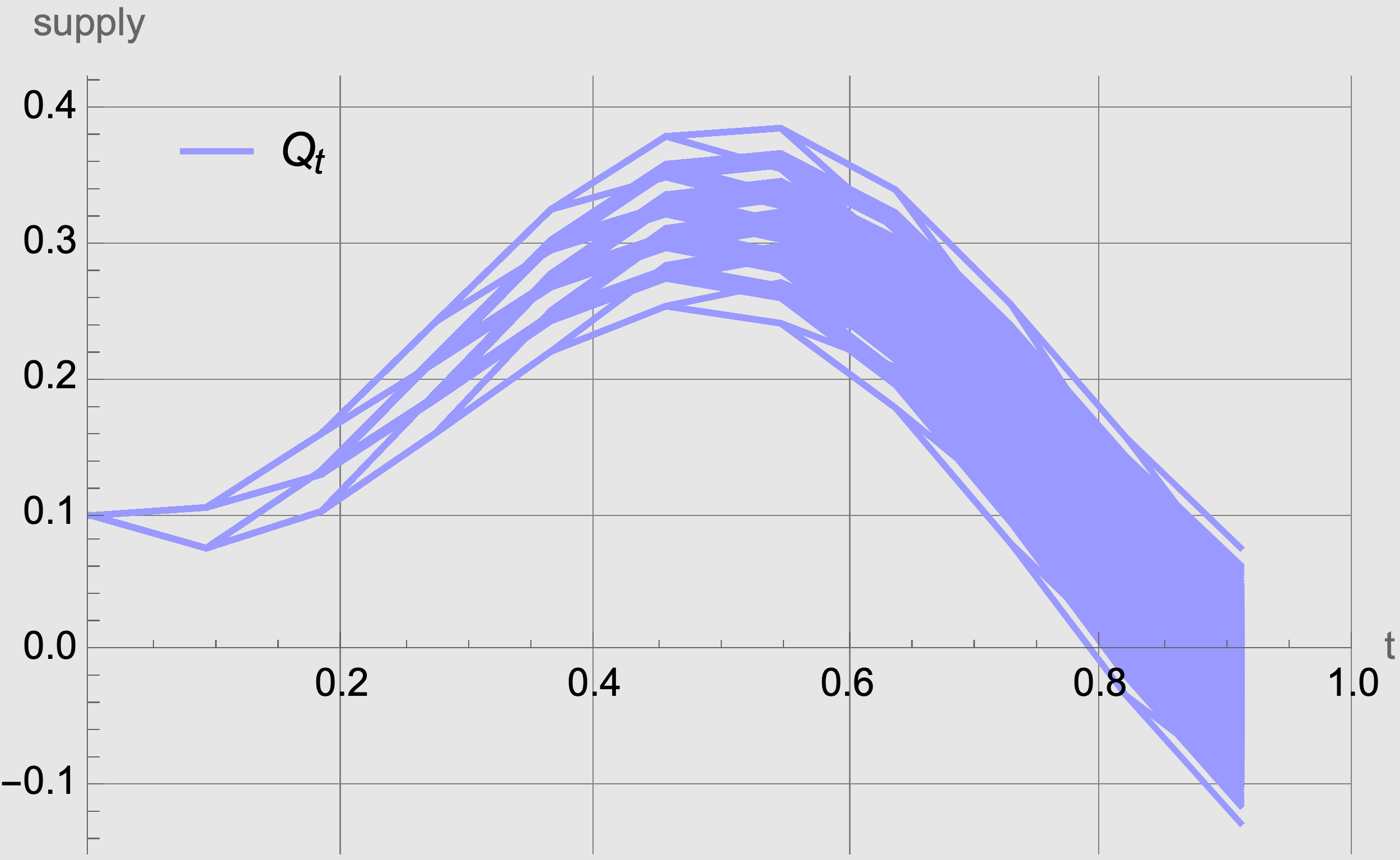
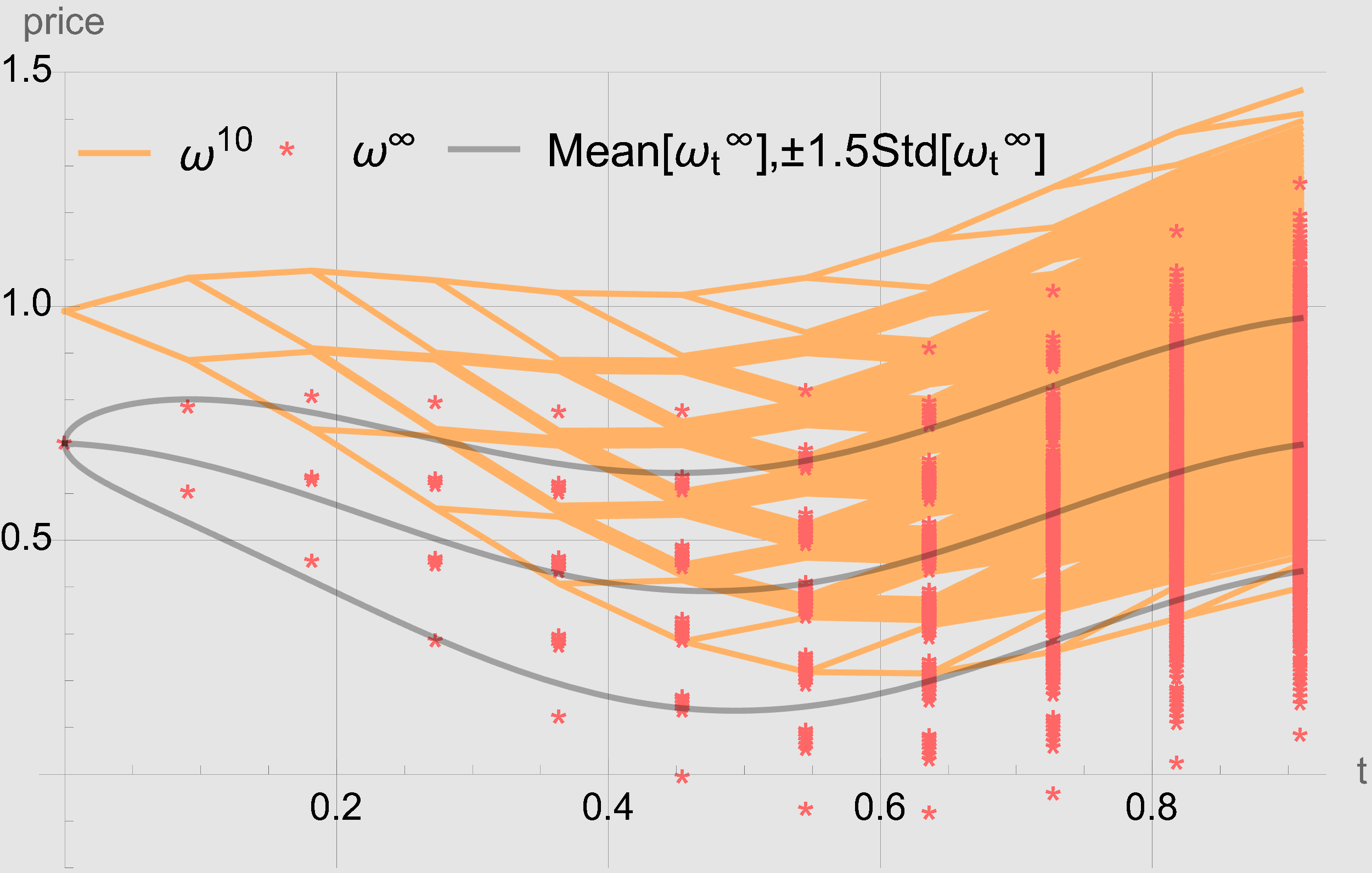
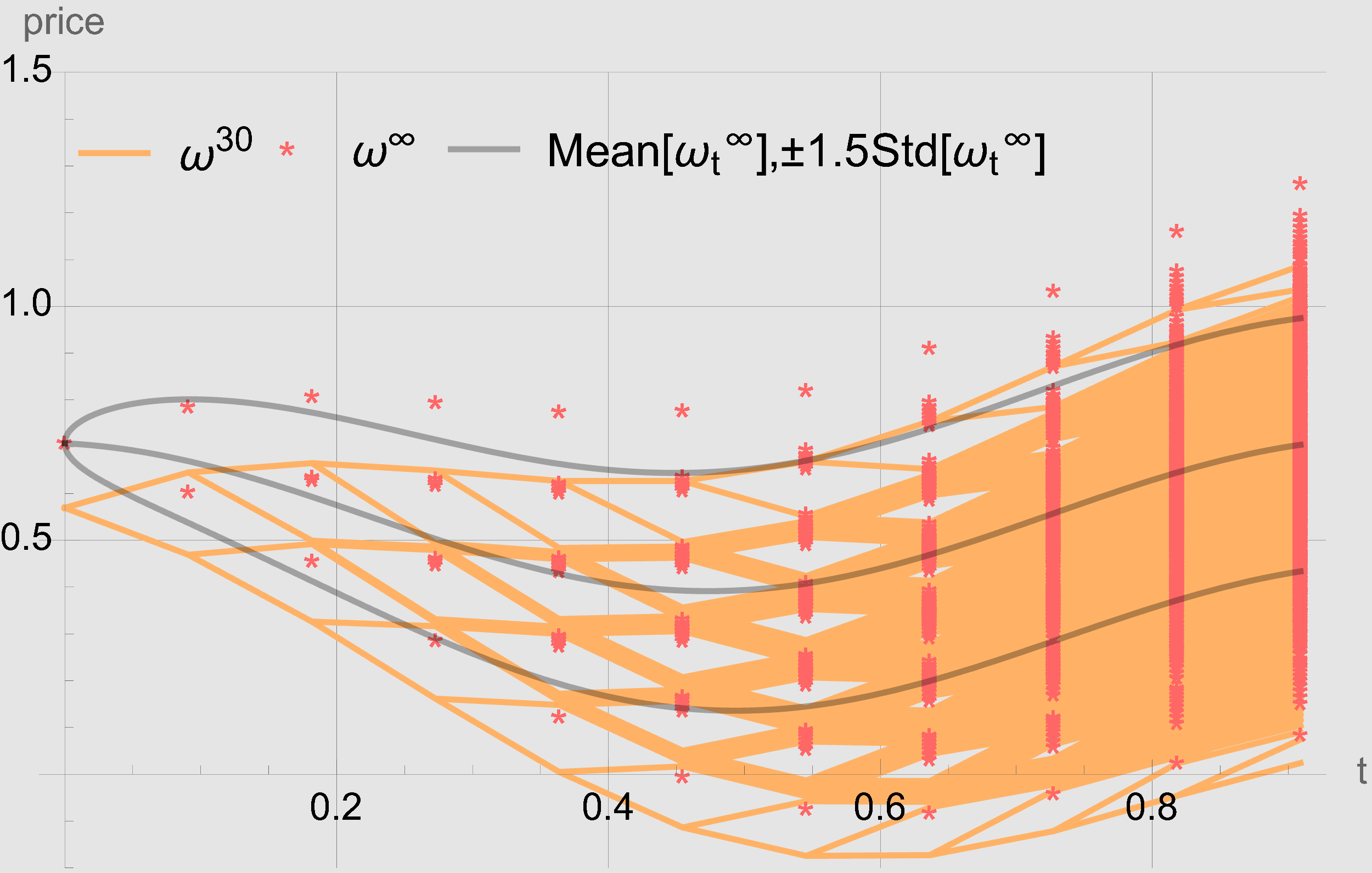
Fig. 2. (Top-left) Binomial tree supply and prices $\varpi^{N}$ and $\varpi^{\infty}$ for $N\in\{10,30,50\}$. Statisticis of $\varpi^{\infty}$ (gray curves).

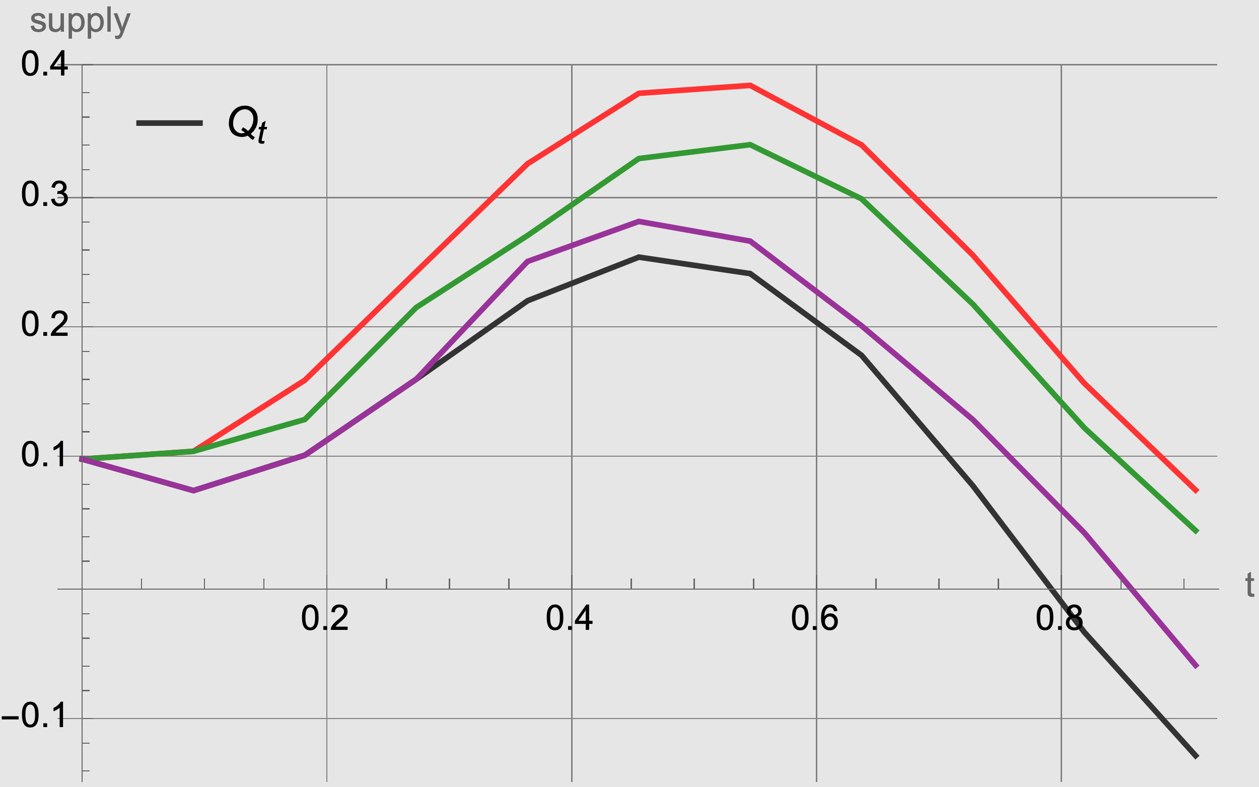
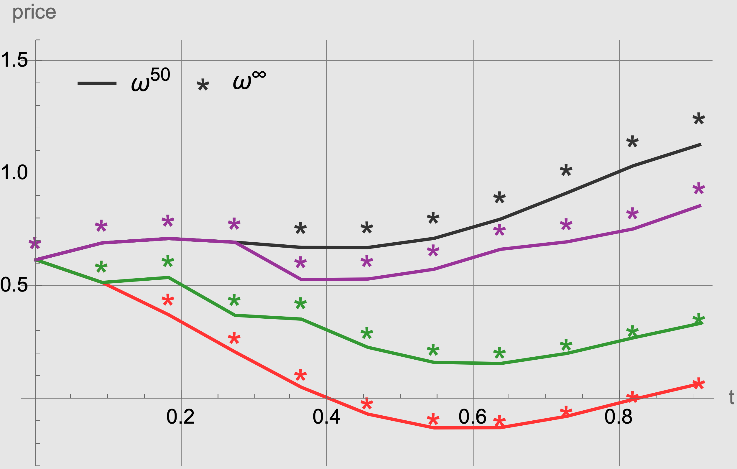
Fig. 3. (Left) Sample trajectories of the supply. (Right) Corresponding prices $\varpi^{N}$, for $N=50$, and $\varpi^{\infty}$ (right).

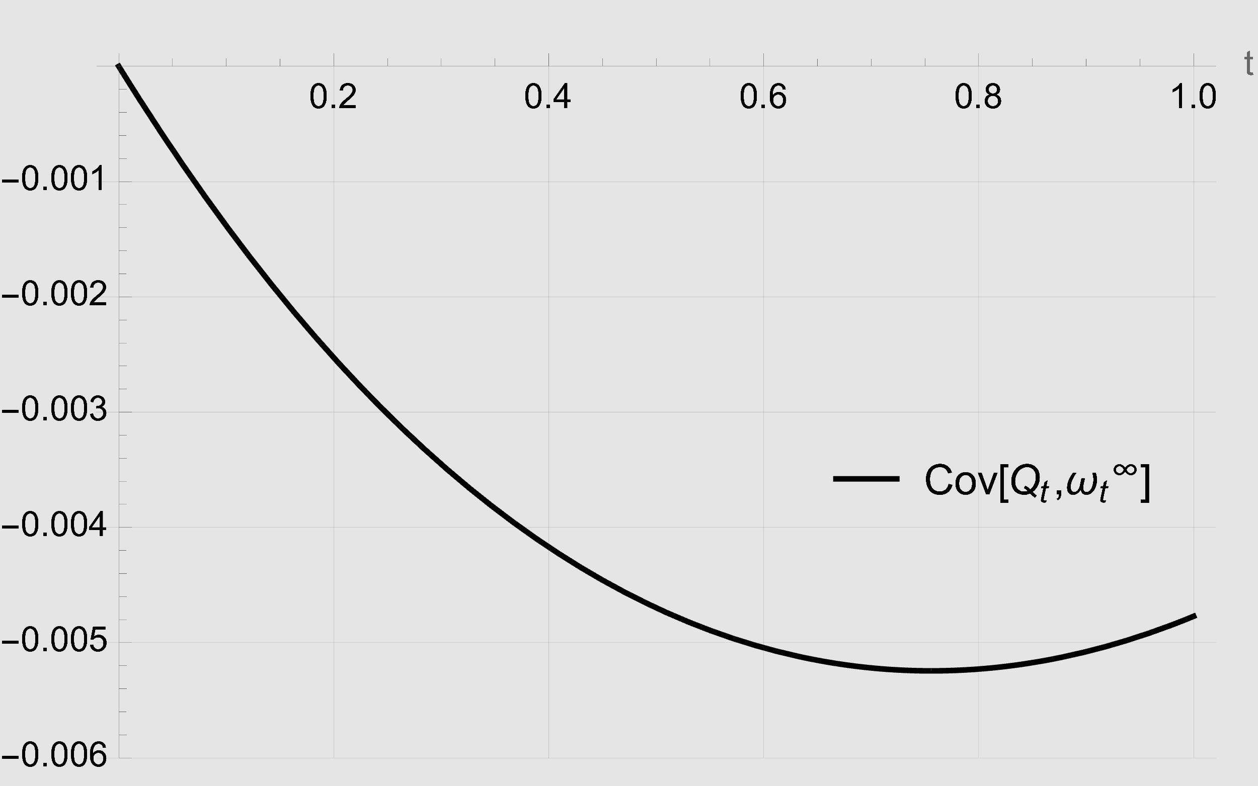
Fig. 4. Covariance between $Q$ and $\varpi^{\infty}$.

6.3. Real data test

Here, we parametrize the linear-quadratic model of Section 5 using real data from the electric grid in Spain. Using the parameterized model, we illustrate the prices obtained from the continuum game.

We use the data of consumption and price from the market in Spain. The data is available at the website https://www.esios.ree.es. We use the hourly demand (megawatts) for the working days of March 2022, so $T=24$ hours. Recall that in our model, both the instantaneous supply $Q$ and the agents provide electricity to the grid, as we assume that each agent has a device storing $X_{t}$ units of electricity at time $t$, which can be further stored or traded in the market. On the contrary, in the electricity grid represented by the real data, agents consume electricity, and no interaction with the market takes place. Therefore, the supply $Q$ we take for our model corresponds to minus the demand observed in the data.

First, we parametrize the supply function. To do so, we assume it is given by

$$Q_{t}=Q_{osc}(t)+Q^{W}_{t},$$ (6.11)

where $Q_{osc}:[0,T]\to{\mathbb{R}}$ and

$$dQ^{W}_{t}=\theta\left(\overline{Q}-Q^{W}_{t}\right)dt+\sigma_{s}dW_{t},$$ (6.12)

for some $\theta,\overline{Q},\sigma_{s}\in{\mathbb{R}}$. Therefore, $Q$ follows the linear dynamics (5.10) for

$$b_{0}^{S}(t)=\dot{Q}_{osc}(t)+\theta\left(\overline{Q}-Q_{osc}(t)\right),\quad b_{1}^{S}(t)=-\theta,\quad\sigma_{0}^{S}(t)=\sigma_{s},\quad\sigma_{1}^{S}(t)=0.$$

We fit $Q_{osc}$ using the mean supply of the data set. Assuming that $Q_{osc}$ is a linear combination of sines and cosines, we obtain

$$Q_{osc}(t)= 0.883118\sin(2\pi t)+0.675294\sin(4\pi t)+0.190316\sin(6\pi t)+0.0248343\sin(8\pi t)$$

$$+0.750615\cos(2\pi t)-0.25301\cos(4\pi t)-0.0233308\cos(6\pi t)+0.191395\cos(8\pi t)$$

$$-0.027736.$$

Because the left-hand side of (6.11) corresponds to the observed data, we fit the parameters $\theta$, $\overline{Q}$, and $\sigma_{s}$ using the maximum-likelihood estimator of (6.12) (see [10], Chapter 3) with time step $h=1/23=0.0434783$. We obtain

$$\theta=35.9957,\quad\overline{Q}=-0.0186653,\quad\sigma_{s}=0.860584.$$

For the initial value of the supply, we take $q_{0}=Q_{osc}(0)+Q^{W}_{0}$, where $Q^{W}_{0}$ is the mean of the observed differences $Q_{0}-Q_{osc}(0)$. Figure 5 depicts the (normalized) supply data and the parameterized supply function. Next, we fit the parameters of the cost functions in (5.1). To do so, we use the expression for the deterministic linear-quadratic model in [24]. In this setting, the MFG price is

$$\varpi(t)=\eta\left(\kappa-\mu_{0}\right)(T-t)+\gamma\left(\zeta-\mu_{0}\right)-\eta\int_{t}^{T}\int_{0}^{s}Q(r)dr\;ds-\gamma\int_{0}^{T}Q(s)ds-cQ(t).$$

We take $Q=Q_{osc}$ in the previous expression, and we fit the parameters using the mean price of the data and least-squares. We obtain

$$\eta=0.00176489,\;\kappa=-371.936,\;c=0.472603,$$

$$\gamma=0.000877786,\;\zeta=377.536,\;\mu_{0}=1.74687.$$

Then, we can compare the observed price data with the corresponding trajectory of the price $\varpi^{\infty}$ obtained in (5.14). Given a supply trajectory from the data $Q^{j}$, we use (6.11), (6.12), and (6.1) to compute the corresponding noise trajectory $\Delta W_{k}^{j}$,

$$\Delta W^{j}_{k}=\frac{Q_{k+1}^{j}-Q_{k}^{j}-hb^{S}(Q_{k}^{j},k)}{\sigma^{S}(Q_{k}^{j},k)},\quad k=0,\ldots,23,$$

which we use in (5.14). Figure 5 depicts three price trajectories.

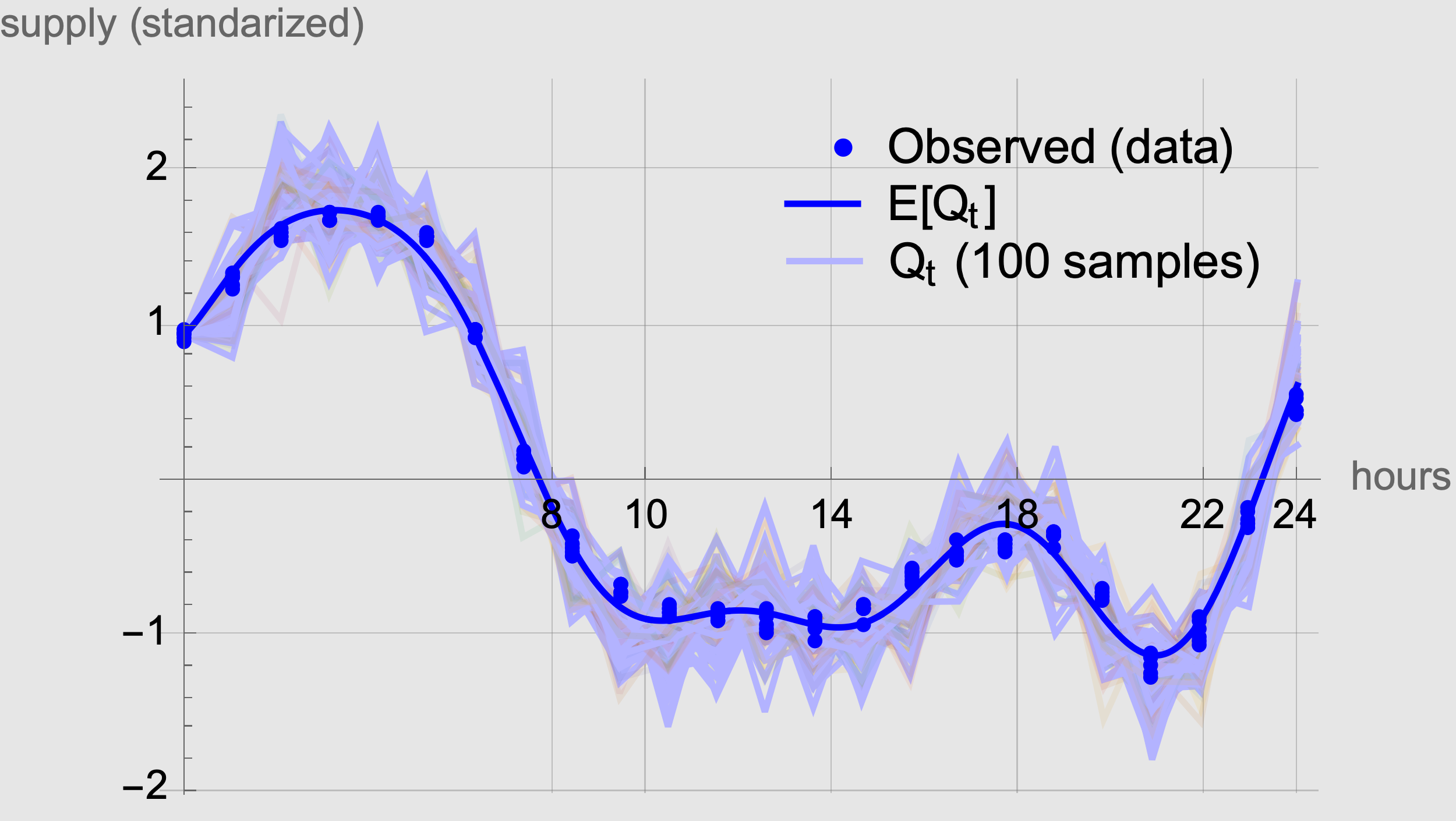
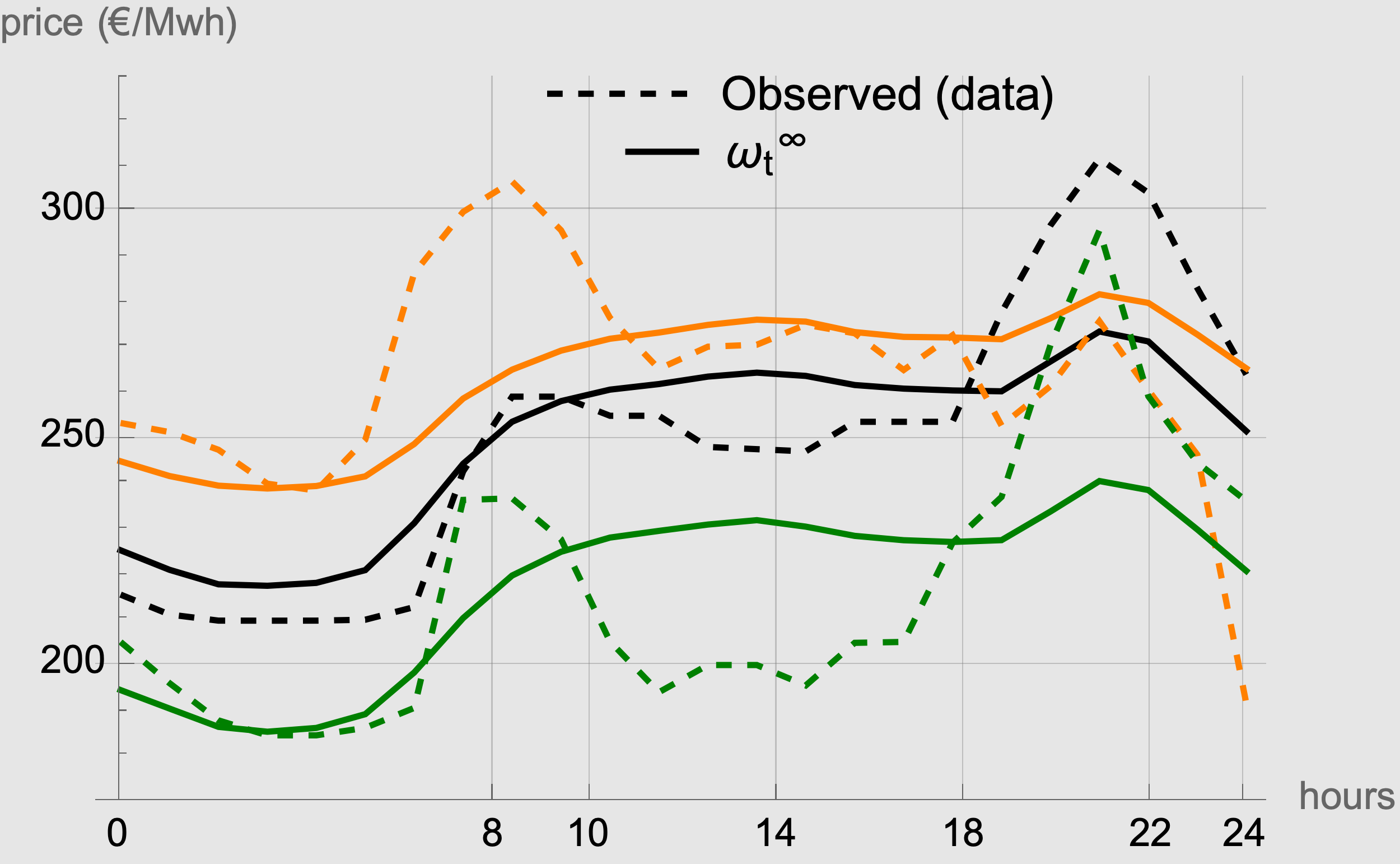
Fig. 5. (Left) Observed supply (data) and simulated supply. (Right) Observed price (3 data samples) and corresponding simulated price $\varpi^{\infty}$.

We observe that price peaks are smoothed, and price variations are reduced. Thus, the price formation mechanism dumps the volatility effect coming from the supply side, and the market may benefit from the smoothing effect. For instance, in June 2021, the Spanish electric introduced voluntary prices for small consumers. The tariffs distinguish three regimes: The peak period (10-14 hrs, 18-22 hrs), the flat period (8-10 hrs, 14-18 hrs, 22-24 hrs), and the valley period (24-8 hrs). The prices are published for the following day, so consumers can decide when to consume energy. If this policy is implemented on a big scale, our price formation model will provide an alternative to balance the different tariffs across regimes.

7. Conclusions and further directions

A price formation model for a finite number of agents is presented. This model corresponds to the particle approximation of the continuum model introduced in [24]. Under convexity and growth assumptions on the cost functions, we proved the solvability of Problem 1. We presented an approach for the numerical solution of the model with a continuum population and another approach for the finite population model.

The approach for the numerical solution of the continuum game uses the Hamilton-Jacobi equation that corresponds to the stochastic optimal control problem that each agent solves. In this case, we characterize the price as the solution of an SDE, whose initial condition (the price value at initial time) admits an explicit expression. Therefore, the error in the approximation depends only on the discrete scheme used to approximate the solution of such SDE. In particular, we use a Forward-Euler scheme, for which the error depends on the time-step size, which can be arbitrarily small without high computational cost due to the explicit nature of the forward scheme. This approach is developed for the linear-quadratic structure of the supply and cost functions.

The approach for the numerical solution of the finite game is suited for any convex cost structure and any supply dynamics. Here, we implement it for the linear-quadratic case only. It relies on the binomial tree approximation of the noise present in the SDE for the supply. As a result, the price is characterized as the Lagrange multiplier of a high-dimensional convex optimization problem with constraints. In this case, as the time-step size decreases, the number of variables in the optimization problem grows exponentially. Therefore, we can not overcome the curse of dimensionality in implementing this approach. However, the results are in good agreement with the theoretical ones.

The qualitative properties of the price obtained by our schemes agree with what is observed in several markets. Fluctuations in the supply are negatively correlated with the price. For the linear-quadratic setting, two relations are observed in the drift of the price: increasing the running trading rate costs $c$ forces the price to move opposite to the supply dynamics, and the price increases when the time-average supply exceeds the preferred running state $\kappa$ of the agents. Moreover, because essentially, the drift determines the expected value of the price, and the volatility determines its variability, we see that the relation between the time-average supply and the preferred state of the agents determines the mean price, while increments on the trading cost increase the variability of the price. Finally, our model provides the scenario for which market saturation results in negative prices.

Other approaches, such as Machine Learning, can be implemented to deal with the high-dimensional nature of Problem 1 as the number of players increases.

In our model, the supply of the commodity is an exogenous process; that is, the supply is an input quantity for the model. A further extension is to consider a supply that depends on the price. In this case, both supply and price would be endogenous variables for the model, and they would be determined by the optimal interaction of agents with the market.

References

- [1] R. Aïd, A. Cosso, and H. Pham. Equilibrium price in intraday electricity markets, 2020.
- [2] R. Aïd, R. Dumitrescu, and R. Tankov. The entry and exit game in the electricity markets: A mean-field game approach. Journal of Dynamics & Games, 8(4):331–358, 2021.
- [3] C. Alasseur, I. Ben Taher, and A. Matoussi. An extended mean field game for storage in smart grids. Journal of Optimization Theory and Applications, 184(2):644–670, 2020.
- [4] C. Alasseur, L. Campi, L. Dumitrescu, and J. Zeng. Mfg model with a long-lived penalty at random jump times: application to demand side management for electricity contracts, 2021.
- [5] A. Alharbi, T. Bakaryan, R. Cabral, S. Campi, N. Christoffersen, P. Colusso, O. Costa, S. Duisembay, R. Ferreira, D. Gomes, S. Guo, J. Gutierrez, P. Havor, M. Mascherpa, S. Portaro, R. Ricardo de Lima, F. Rodriguez, J. Ruiz, F. Saleh, S. Calum, T. Tada, X. Yang, and Z. Wróblewska. A price model with finitely many agents. Bulletin of the Portuguese Mathematical Society, 2019.
- [6] T. Basar and R. Srikant. Revenue-maximizing pricing and capacity expansion in a many-users regime. In Proceedings.Twenty-First Annual Joint Conference of the IEEE Computer and Communications Societies, volume 1, pages 294–301 vol.1, 2002.
- [7] H. H. Bauschke, P. L. Combettes, et al. Convex Analysis and Monotone Operator Theory in Hilbert Spaces. CMS Books in Mathematics. Springer International Publishing, 2 edition, 2017.
- [8] P. Billingsley. Probability and Measure, Third Edition (Wiley Series in Probability and Statistics). Wiley Series in Probability and Statistics. Wiley-Interscience, 3 edition, 1995.
- [9] S. Boyd and L. Vandenberghe. Convex Optimization. Cambridge University Press, USA, 2004.
- [10] D. Brigo and Mercurio F. Interest Rate Models - Theory and Practice. Springer Finance. Springer, 2nd edition, 2006.
- [11] P. Cannarsa and C. Sinestrari. Semiconcave functions, Hamilton-Jacobi equations, and optimal control. Progress in Nonlinear Differential Equations and their Applications, 58. Birkhäuser Boston, Inc., Boston, MA, 2004.
- [12] R. Carmona and F. Delarue. Probabilistic Theory of Mean Field Games with Applications I-II. Springer, 2018.
- [13] B. Dacorogna. Introduction to the calculus of variations. Imperial College Press, London, third edition, 2015.
- [14] B. Djehiche, J. Barreiro-Gomez, and H. Tembine. Price Dynamics for Electricity in Smart Grid Via Mean-Field-Type Games. Dynamic Games and Applications, 10(4):798–818, December 2020.
- [15] N. El Karoui, S. Peng, and M. C. Quenez. Backward stochastic differential equations in finance. Mathematical Finance, 7(1):1–71, 1997.
- [16] D. Evangelista, Y. Saporito, and Y. Thamsten. Price formation in financial markets: a game-theoretic perspective, 2022.
- [17] L. C. Evans. Partial Differential Equations. Graduate Studies in Mathematics. American Mathematical Society, 1998.
- [18] O. Féron, P. Tankov, and L. Tinsi. Price Formation and Optimal Trading in Intraday Electricity Markets with a Major Player. Risks, 8(4):1–1, December 2020.
- [19] O. Féron, P. Tankov, and L. Tinsi. Price formation and optimal trading in intraday electricity markets, 2021.
- [20] M. Fujii and A. Takahashi. A Mean Field Game Approach to Equilibrium Pricing with Market Clearing Condition. Papers 2003.03035, arXiv.org, March 2020.
- [21] M. Fujii and A. Takahashi. Equilibrium price formation with a major player and its mean field limit, 2021.
- [22] D. Gomes, J. Gutierrez, and R. Ribeiro. A mean field game price model with noise. Math. Eng., 3(4):Paper No. 028, 14, 2021.
- [23] D. Gomes, L. Lafleche, and L. Nurbekyan. A mean-field game economic growth model. Proceedings of the American Control Conference, 2016-July:4693–4698, 2016.
- [24] D. Gomes and J. Saúde. A Mean-Field Game Approach to Price Formation. Dyn. Games Appl., 11(1):29–53, 2021.
- [25] A. C. Kizilkale and R. P. Malhamé. A class of collective target tracking problems in energy systems: Cooperative versus non-cooperative mean field control solutions. In 53rd IEEE Conference on Decision and Control, pages 3493–3498, 2014.
- [26] A. J. Kurdila and M. Zabarankin. Convex functional analysis. Springer Science & Business Media, 2006.
- [27] J. Ma and J. Yong. Forward-Backward Stochastic Differential Equations and Their Applications. Lecture Notes in Mathematics. Springer, corrected edition, 2007.
- [28] B. Øksendal. Stochastic differential equations. Universitext. Springer-Verlag, Berlin, sixth edition, 2003. An introduction with applications.
- [29] H. Shen and T. Basar. Pricing under information asymmetry for a large population of users. Telecommun. Syst., 47(1-2):123–136, 2011.
- [30] A. Shrivats, D. Firoozi, and S. Jaimungal. A Mean-Field Game Approach to Equilibrium Pricing, Optimal Generation, and Trading in Solar Renewable Energy Certificate Markets. Papers 2003.04938, arXiv.org, March 2020.
- [31] N. Touzi. Optimal Stochastic Control, Stochastic Target Problems, and Backward SDE, volume 29. Springer-Verlag New York, 2013.
- [32] Jiongmin Yong. Linear forward-backward stochastic differential equations with random coefficients. Probability Theory and Related Fields, 135(1):53–83, 2006.