The Impact of Algorithmic Risk Assessments on Human Predictions and its Analysis via Crowdsourcing Studies

Abstract.

As algorithmic risk assessment instruments (RAIs) are increasingly adopted to assist decision makers, their predictive performance and potential to promote inequity have come under scrutiny. However, while most studies examine these tools in isolation, researchers have come to recognize that assessing their impact requires understanding the behavior of their human interactants. In this paper, building off of several recent crowdsourcing works focused on criminal justice, we conduct a vignette study in which laypersons are tasked with predicting future re-arrests. Our key findings are as follows: (1) Participants often predict that an offender will be rearrested even when they deem the likelihood of re-arrest to be well below 50%; (2) Participants do not anchor on the RAI’s predictions; (3) The time spent on the survey varies widely across participants and most cases are assessed in less than 10 seconds; (4) Judicial decisions, unlike participants’ predictions, depend in part on factors that are orthogonal to the likelihood of re-arrest. These results highlight the influence of several crucial but often overlooked design decisions and concerns around generalizability when constructing crowdsourcing studies to analyze the impacts of RAIs.

1. Introduction

Risk assessment instruments (RAIs) are increasingly deployed in critical domains, including finance, education, criminal justice, child welfare, hiring, and healthcare (Paravisini and Schoar, 2013; Delen, 2010; Berk et al., 2018; Saxena et al., 2020; Sendak et al., 2020; Raghavan et al., 2020). Rationales for adopting these tools often center around efficiency: The hope is that RAIs might offer fast, accurate, objective, and cheap decision-making at scale (Metz and Satariano, 2020). To assess the potential benefits and disadvantages of RAIs, common practice is to compare their statistical properties against the status quo. However, while most research on algorithmic fairness, accountability, and transparency has focused on RAIs in isolation, a broad recognition is emerging, particularly within the HCI community, that many of these tools must be studied as situated in human-in-the-loop systems.

While it can be challenging to assess the predictive performance and fairness properties of RAIs in isolation (Kleinberg et al., 2017; Kallus and Zhou, 2019; Lakkaraju et al., 2017; Fogliato et al., 2020; Coston et al., 2021), investigating their impact on systems where the human is the ultimate decision maker introduces a new layer of complexity. Perhaps the most direct evidence bearing on these questions comes from longitudinal studies of real-world systems (De-Arteaga et al., 2020; Chouldechova et al., 2018), particularly within the criminal justice setting. Several such studies have argued that these RAIs did not substantially improve the quality of the judicial decisions (Stevenson, 2018; Berk, 2017) and in some cases amplified the existing disparities (Albright, 2019). In studies that reported more positive outcomes, the RAI was often deployed as part of broader criminal justice reforms, making it difficult to isolate the effect of the algorithmic tool from other explanatory factors (Grant, 2019; Austin and Ware, 2020).

In order to overcome the difficulties of characterizing decision-making and the impact of RAIs on systems where the human is in-the-loop, many researchers have turned to lab experiments (Yin et al., 2019; Poursabzi-Sangdeh et al., 2021; Zhang et al., 2020; Bansal et al., 2021). Findings from these studies, however, may not generalize to real-world high-stakes contexts because study participants, who are typically recruited on crowdsourcing platforms, are not representative of experts and because, unlike experts, they are not actually making decisions (only predictions). Still, results from these studies can elucidate general phenomena that characterize human-in-the-loop decision-making frameworks. In addition, the predictive performance achieved by study participants can arguably be seen as a benchmark for expert decision makers.

Many studies in this line of research have focused on the criminal justice context (Dressel and Farid, 2018; Biswas et al., 2020; Green and Chen, 2019a; Grgić-Hlača et al., 2019; Green and Chen, 2019b; Jung et al., 2020; Mallari et al., 2020). These works have mainly examined predictive performance and fairness properties concerning the study participants’ predictions of defendants’ future criminal recidivism, often using the ProPublica COMPAS dataset (Angwin et al., 2016). However, their survey designs exhibit several key differences, such as as the number and type of predictions elicited from participants, the structure of financial rewards, and the requirements participants had to satisfy to take part in the study (longer discussion in §2).

In this paper, we first characterize some of the aforementioned differences across survey designs and then introduce our empirical study to determine how these factors impact crowdworkers’ predictions of future criminal recidivism. More specifically, we identify four research questions (RQs) that we believe are important considerations for assessing the generalizability of results from these studies but, to our knowledge, have not been addressed by prior work:

RQ1:

Do evaluations of participants’ responses depend on the type of predictions that are elicited? More specifically, can we infer participants’ (binary) outcome predictions only based on their (probability) risk estimates? Does this matter for evaluations of participants’ predictive performance and reliance on the RAI?

RQ2:

What is the impact of anchoring effects on participants’ predictions? In other words, do participants respond differently if they are asked to pre-register provisional responses before being shown the RAI’s recommendation?

RQ3:

How much time do participants spend on the assessments?

RQ4:

How do predictions (of re-arrest) and judicial decisions (to incarcerate) differ?

To investigate RQ1–4, we designed a vignette study (the “survey”) where laypersons recruited on Amazon Mechanical Turk were asked to predict future recidivism of a series of criminal offenders with and without the assistance of an RAI (see §3). Participants were shown short descriptions of the offenders and then asked to assess the likelihood and predict whether the given offenders would be rearrested. By employing a between-subjects design, we tested whether participants anchored on the RAI’s recommendations when these were presented at the outset together with the offender’s description.

Our results (§4) indicate the importance of asking participants separately about their probability predictions and their (binary) outcome predictions: (1) The study participants often predicted re-arrest even when they deemed the likelihood of re-arrest to be well below 50%. The distinction matters for evaluations of participants’ predictive performance and reliance on the RAI. For example, we find that participants substantially updated their risk estimates in the direction of the RAI’s recommendation, but they rarely revised their binary predictions to match the RAI’s (binary) prediction. Interestingly, participants self-reported revising their risk estimates almost twice as often as their binary predictions after seeing the RAI’s recommendation. (2) Interestingly, we do not find any evidence of participants anchoring on the RAI’s predictions. Instead, surprisingly, the revised risk estimates made by participants in our non-anchoring condition were significantly closer to the RAI’s. (3) By tracking the time spent on each vignette, we discover that many participants take a long time to complete the survey but actually spend surprisingly little time on each case (average=15 seconds, median=10), taking long breaks. Moreover, because many participants perform similarly and few outperform the RAI, their predictive accuracy does not constitute a reliable proxy of time spent. (4) Finally, we discuss crucial differences between the predictive task and judicial decisions that make it difficult to draw direct conclusions about the latter from crowdsourcing studies such as ours. We present an analysis of real judicial decisions, which suggests that judicial decisions, unlike participants’ predictions, depend not only on the offender’s likelihood of recidivism but also on the gravity of the crimes committed.

To facilitate the reproducibility of our analysis, we have obtained IRB approval from Carnegie Mellon University and participants’ consent to publicly share the data collected as part of our experiment. Our data and code for the analysis are available at www.github.com/ricfog/the-impact-of-algorithmic-rais.

2. Background

We focus our treatment of related work primarily on crowdsourcing studies on the prediction of criminal recidivism (Dressel and Farid, 2018; Biswas et al., 2020; Tan et al., 2018; Green and Chen, 2019a; Grgić-Hlača et al., 2019; Green and Chen, 2019b; Jung et al., 2020; Mallari et al., 2020). These studies mainly involve related prediction tasks in which participants are asked to predict the likelihood that a defendant or an offender, if released, will be rearrested within a specified period of time. Factors that would likely influence decisions but not predictions, such as the defendant’s ability to pay bail or their culpability, are intentionally excluded. Factors that are not recorded in the data used by the RAI, such as the defendant’s and prosecutor’s arguments, are also (necessarily) left out. These studies speak to the gains in efficiency that should be expected if judges were to make decisions only based on the defendant’s likelihood of re-arrest and the information present in the data. As our analysis will show (see §4.4), these results do not directly inform the impact of future deployments of RAIs; yet, they potentially provide a benchmark for the predictive performance of these human-in-the-loop systems.

Existing studies have mainly focused on two key questions: (i) how the predictions of study participants (alone) compare to the RAI’s; and (ii) whether and how the RAI’s recommendations are taken into account by participants. In terms of the former, the influential study of Dressel and Farid (2018) found that, on the ProPublica COMPAS dataset (Angwin et al., 2016), the predictive accuracy of their study participants’ (crowdworkers) was comparable to that of the COMPAS RAI. The authors concluded that laypersons performed no worse than COMPAS. Successive studies replicated this finding (Jung et al., 2020; Mallari et al., 2020; Grgić-Hlača et al., 2019). However, they also found that participants’ predictive performance was considerably lower than the RAI’s when outcome feedback was removed, the base rate was decreased, or when the area under the curve (AUC), instead of accuracy, was considered (Jung et al., 2020). These results should not be surprising for two reasons. First, humans tend to ignore information about the base rate, a phenomenon known as “base rate neglect” (O’Hagan et al., 2006; Koehler, 1996). This bias, however, is mitigated when outcome feedback is provided (Gluck and Bower, 1988). Second, even simple RAIs achieve predictive accuracy similar to that of COMPAS (Angelino et al., 2017), but ranking offenders by their risk of recidivism (i.e., regression) represents a “harder” statistical problem. Studies in the second line of work, which investigated human predictions in presence of the RAI, generally found that the RAI led to small or no increments in the predictive performance of participants’ predictions (Vaccaro and Waldo, 2019; Green and Chen, 2019b). Two related studies observed differential compliance with the RAI’s recommendations across defendants’ racial groups: They found that providing participants with the RAI’s prediction led to a larger increase in the predicted risk of re-arrest for Black defendants compared to White defendants (Green and Chen, 2019a, b), a phenomenon that the authors named “disparate interactions”. In our study, we found that participants, when presented with the RAI’s recommendations, performed worse than the RAI across all the metrics that we considered (§B.1). In addition, we note that we were not able to replicate the disparate-interactions effect (§B.3).

However, some of the survey designs employed by these experiments present notable differences. In the following paragraphs, we describe some of such differences and discuss, based on both past and our own work, how these design choices can impact the predictions made by study participants.

In eliciting predictions, some studies asked participants for their risk estimates (probabilities) (Green and Chen, 2019a; Jung et al., 2020), whereas others asked for (binary) outcome predictions of re-arrest (Dressel and Farid, 2018; Mallari et al., 2020). Vaccaro and Waldo (2019) collected both and Grgić-Hlača et al. (2019) had participants provide confidence ratings. To derive binary predictions from risk estimates, Jung et al. (2020) assumed that participants would have predicted re-arrest for a defendant whenever their risk estimate was larger than 50%. However, it is well known that many individuals, even expert decision makers, can struggle with poor numeracy skills (Black et al., 1995; Schwartz et al., 1997; Lipkus et al., 2001; Visschers et al., 2009). In addition, individuals may base their decisions on a distorted version of the estimate of the risk, e.g., by overweighting small probabilities (Kahneman and Tversky, 2013; Prelec, 1998). One recent crowdsourcing study on uncertainty visualization has found that individuals that were poor at probability judgments did well on decision tasks (Kale et al., 2020). Consistent with this evidence, our results support the hypothesis that participants’ binary predictions cannot be simply obtained by converting risk estimates at a fixed threshold (§4.1).

Past studies also differ in the stage at which the RAI’s recommendation was presented to the participants. In one of these studies (Green and Chen, 2019a), the defendant’s description and the RAI’s recommendation were presented to participants at the same time. In another (Grgić-Hlača et al., 2019), the RAI’s information was made available only after the participant had made an initial prediction. However, the psychology and behavioral economics literature suggest that participants might rely on the RAI more heavily in the former setting due to a phenomenon known as the anchoring effect, a.k.a. “anchoring and adjustment heuristic” (O’Hagan et al., 2006; Tversky and Kahneman, 1974; Epley and Gilovich, 2005). According to this heuristic, participants that are presented with a novel “anchor” would first try to assess whether the anchor equals the target and then adjust its value. The final answer generally tends to be biased in the direction of the anchor. In the setting of our study, anchor and target are represented by the RAI’s recommendation and the defendant’s recidivism outcome respectively. Since individuals are often unable to accurately describe their own cognitive mental processes (Nisbett and Wilson, 1977; Wilson, 2004), hypotheses around this phenomenon need to be empirically tested. This cognitive bias has been shown to affect judicial decision-making (Enough and Mussweiler, 2001; Englich et al., 2005, 2006; Mussweiler and Strack, 2000; Bushway et al., 2012) and it has been studied in at least three other crowdsourcing experiments (Vaccaro and Waldo, 2019; Green and Chen, 2019b; Buçinca et al., 2021), two of which focused on recidivism RAIs. Close to our work is Green and Chen (2019b), which examined the effect of anchoring on participants’ risk estimates, finding that participants that had pre-registered their answers achieved higher predictive performance. In our experiment, performance was nearly identical across the two settings. Surprisingly, we found no evidence of anchoring bias: The risk estimates made by the participants that had to pre-register their predictions before seeing the RAI’s recommendations were closer to the predictions made by the RAI (§4.2).

The studies also differ considerably in the number of defendants’ profiles that were shown, the requirements that workers had to satisfy in order to participate, the structure of the financial compensation, the number and form of attention checks. These factors likely impacted the amount of effort made by participants in the study. But none of the studies has tried to quantify the effort that participants make on each prediction, an aspect that seems especially important for ecological validity. Problematically, for these tasks, even participants that answer carefully can achieve low predictive accuracy and thus accuracy may not be a reliable proxy for effort. Alternatively, one might consider the time spent by participants on the entire survey, which many past studies have reported (Green and Chen, 2019a; Vaccaro and Waldo, 2019; Mallari et al., 2020; Grgić-Hlača et al., 2019). By taking into account the number of defendants shown in each of these surveys, a quick computation suggests that, on average, the prediction for a single defendant may take less than 15 seconds. In our study, we show that, while this actually corresponds to the average time spent by our survey participants on each of the assessments, it varies widely both across participants and across vignettes (median=10 seconds) (§4.3).

Another difference in survey designs that is worth mentioning, but whose consequences we don’t explore in this work, is the type of the RAI’s recommendation that was displayed in the vignette. In past studies, participants were presented with the raw risk estimate of the RAI (Green and Chen, 2019a), the prediction binned into risk scores (Vaccaro and Waldo, 2019), or just the binary prediction (Grgić-Hlača et al., 2019). The type of RAI’s prediction that is communicated has been shown to impact participants’ judgments in crowdsourcing studies (Lai and Tan, 2019; Zhang et al., 2020) and even decisions made in the criminal justice context (Scurich and John, 2011). In §4.1, we show that participants often do not revise their binary prediction in the direction of the RAI’s. In contrast, Grgić-Hlača et al. (2019) found that when study participants revised their (binary) predictions, they did so to match the RAI’s in almost the majority of cases. In light of our results around how people convert risk estimates into binary predictions, the seeming contrast between the two results is likely attributable to our design choice of providing participants only with the RAI’s risk estimate and not its binary prediction.

We now focus on one last important difference: the target of the studies. As we mentioned before, the goal of some of these experiments was to compare the predictive performance of the RAI with that of laypersons (Dressel and Farid, 2018; Jung et al., 2020). The goal of other studies was, instead, to highlight potential unintended consequences arising from the use of RAIs in judicial decision-making (Grgić-Hlača et al., 2019; Green and Chen, 2019a). However, there is a clear disconnect between predictions of re-arrest, which were collected through the surveys, and decisions (e.g., of whether to incarcerate), which are made by judges. In particular, the risk of criminal recidivism, on which participants’ predictions are based, represents only one of multiple factors that judges (are allowed to) account for in their decision-making process. Our results show that these differences cannot be easily reconciled in the criminal sentencing setting, especially in context of sentencing considered in our study (§4.4).

3. Data and methods

This section is organized as follows. First, we provide an overview of the dataset and of the statistical modeling used to develop the RAI (§3.1). We then cover task and experimental design (§3.2), procedure (§3.3), and recruitment process (§3.4). Lastly, we present the methodology used for the analysis of the results (§3.5). In Appendix §E, we also describe a small pilot study that we ran while developing the current experiment. The pilot is different in several ways from the main study, such as in the compensation scheme, which was not tied to performance.

	dataset	survey sample
share of male offenders	79.0%	79.1%
share of White offenders	65.3%	65.1%
number of prior arrests (sd)	3.8 (4.9)	3.8 (4.9)
mean age (sd)	31.2 (10.4)	31.4 (10.3)
mean age of first arrest (sd)	23.5 (8.6)	23.5 (8.6)
prevalence of re-arrests	41.9%	42.0%
number of offenders	117464	3523

Table 1. Summary statistics for the offenders contained in the full dataset and in the subset of offenders extracted for the survey. Age is measured in years. Standard deviations (“sd”) are reported in parantheses. The marginal distributions of the offenders’ prior number of charges, type of offense committed, and age of first arrest in dataset and survey sample are also similar, but are omitted from the table.

3.1. Data and development of RAI

3.1.1. Data

The set of offenders used in our survey comes from a private dataset provided by the Pennsylvania Commission on Sentencing. The data contain information about offenders sentenced in the state’s criminal courts. In our analysis, we considered only offenders whose race, as recorded in the data, was White or Black. The final dataset consisted of 117,464 observations, 65% of which corresponded to White offenders. For each of the offenders, we know whether they were rearrested within three years from the time of release from prison or imposition of community supervision. The overall base rate was 41.9%, while the re-arrest rates for Black and White offenders were 51% and 37.1%, respectively. We split the full data into train and test sets (70%-30%) prior to model training. A sample of 3,523 observations were further selected from the test set using stratified random sampling to ensure that the resulting sample reflected the test population on race, sex, age, and re-arrest status. These observations were used in the survey. Summary statistics for the dataset and the survey sample are reported in Table 1.

3.1.2. Development of the RAI

We used the available data to train RAIs that predict 3-year post-release re-arrest using demographic features (age, sex, and race), information about the current charge (type of offense and whether it is a misdemeanor or a felony), and several features reflecting prior criminal history (e.g., past number of arrest and charges for several offense categories). We trained logistic regression, Lasso (Tibshirani, 1996), random forest (Breiman, 2001), and extreme gradient boosting (XGBoost) (Chen and Guestrin, 2016) models on the training data, tuning the hyperparameters via cross-validation. The four models showed similar performance on the holdout set: Prediction accuracy was around 66% and the area under the curve (AUC) was approximately 70%. These AUCs are comparable to those of other recidivism RAIs that are deployed in jurisdictions across the country, such as COMPAS (Dieterich et al., 2016) and the Public Safety Assessment (PSA) (DeMichele et al., 2018a), among others (Desmarais et al., 2020). All models were fairly well calibrated overall and, at a classification threshold of 0.5, they all predicted re-arrest for approximately 30% of the offenders in the holdout set. We also assessed the models for racial predictive bias, finding that the Lasso and random forest models were both racially well-calibrated. More details on our assessment of predictive bias in the predictions are provided in §A. Given the similarity in overall performance across the four models, we decided to adopt the Lasso for our experiments, since it was the simplest model that we found to be racially well-calibrated. For this part of the analysis, we used the tidyverse (Wickham et al., 2019) and tidymodels (Kuhn and Wickham, 2020) sets of packages in R (R Core Team, 2019).

3.2. Task and experimental design

In the survey, participants were tasked with predicting the likelihood and the occurrence of a re-arrest for a series of 40 offenders. The profile of each offender was presented through a descriptive paragraph based on a subset of the features that had been used to train the RAI. For each offender, participants were asked the two following questions: ($Q^{p}$) ”What is the likelihood of this offender being rearrested in the three years following release?” and ($Q^{b}$) ”Do you think that the offender was rearrested in the three years following release?”. The possible answers to $Q^{p}$ were probabilities on a scale 0%-100% in bins of $1\%$ which could be selected using a slider scale. The initial value of such slider was randomly set at either 0% or 100% when the participant entered the survey. Instead, $Q^{b}$ required a negative or positive answer which could be selected using radio buttons. Two examples of vignettes are shown in Figure 1 (see also the structure of the vignette in §C.6). The core task in the survey consisted of three consecutive parts, which consisted of $14$, $25$, and $1$ offenders’ assessments respectively (see Figure 2). We now describe each of these in turn.

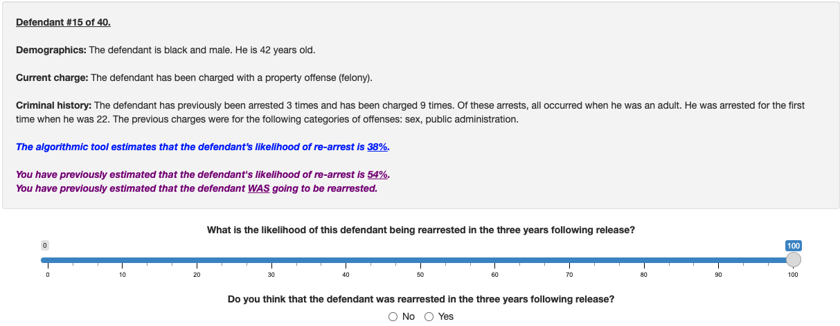
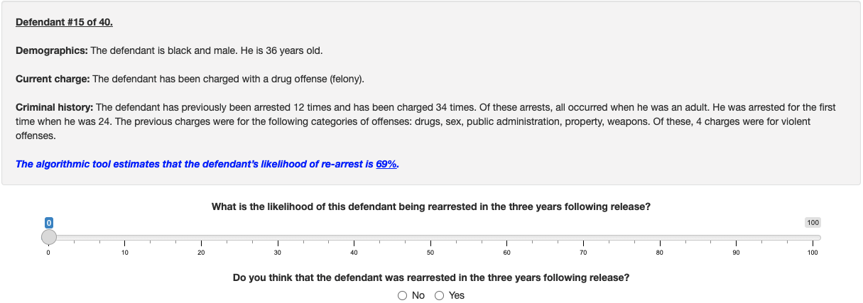
Figure 1. The top and bottom panels provide examples of vignettes that were presented to participants in the non-anchoring and anchoring settings respectively. Participants assigned to the former setting were first asked to pre-register provisional responses that they were allowed to revise after being shown the RAI’s recommendation (example here). Participants assigned to the anchoring setting were shown directly the RAI’s recommendation. Both the likelihood estimate and the binary prediction were required to proceed to the following vignette. The initial value of the slider was randomly set at either 0% or 100%.

In the first part of the survey (offenders #1-14 in Figure 2), participants were provided with outcome feedback, but the RAI’s predictions were not made available to them. Participants were asked to record their responses ($Q^{p}_{P}$ and $Q_{P}^{b}$) and given feedback after each prediction. The feedback was as follows: “The offender was/was not rearrested in the three years following release”, which was shown in green if the participant’s prediction for $Q^{b}$, the binary prediction question, was accurate and in red otherwise. Offenders’ profiles were randomly drawn from the survey sample.

In the second part of the survey (offenders #15-39), outcome feedback was removed but participants were shown the RAI’s predictions. We employed a between-subjects design to study the effect of anchoring, assigning participants to one of two conditions, which we call anchoring and non-anchoring. The participants that were assigned to the anchoring condition were shown the offender’s profile and the prediction of the RAI in the same vignette ($Q^{p}_{P+RAI}$ and $Q_{P+RAI}^{b}$). Here, the RAI serves as the anchor. Instead, if assigned to the non-anchoring setting, participants were first asked to estimate the likelihood ($Q_{P}^{p}$) and predict the occurrence ($Q_{P}^{b}$) of a re-arrest based on the offender’s profile alone, as they had done during the first part of the study. After submitting a response, they were presented with the RAI’s prediction for the given case and were allowed to revise their own predictions ($Q^{p}_{P+RAI}$ and $Q_{P+RAI}^{b}$). The randomization scheme was based on Efron’s biased coin design (Efron, 1971). In this part of the survey, participants were shown the descriptions of a set of offenders that were drawn from the survey sample either randomly or controlling for the RAI’s predictive accuracy to be around 67%. However, due to a glitch, some of the participants were shown all cases for which the RAI’s binary predictions were accurate first. One past work found that the order in which the offenders’ profiles were ordered did not affect participants’ reliance on the RAI, even when outcome feedback was given (Grgić-Hlača et al., 2019). Since the study participants affected by the glitch were equally split across the anchoring and non-anchoring conditions (see Table 2 in §B.4) and we could not detect any interaction of the two effects in some preliminary analysis of the data, we decided to consider their responses in the analysis.

The third and last part of the survey consisted of only one assessment (offender #40), which the participant made right before exiting the survey and was analogous to those in the anchoring setting. Through this assessment, we wished to test any meaningful differences in the predictions of the participants that had been assigned to the two different treatments. We did not find any substantial difference in their responses and consequently we omitted the discussion of these results from the paper.

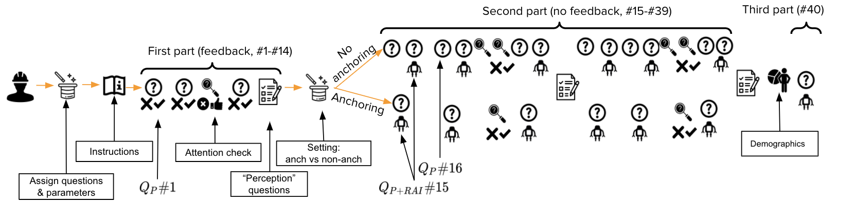
Figure 2. Structure of the survey. $Q_{P+RAI}\#i$ and $Q_{P}\#i$ indicate the answers given by the participant with and without the assistance of the RAI, respectively, for the $i^{th}$ offender. At the initialization of the web app, the offender’s profiles and the other parameters were chosen. Then the participant went through the instructions (see also §C). In the first part of the survey, consisting of 14 offenders plus one attention check, outcome feedback was provided. At the end, the participant completed the “perception questions” and then proceeded to the second part of the survey. Here, the participant did not receive feedback and was assigned to either the anchoring or to the non-anchoring setting. This part consisted of 25 offenders (#15-39) plus two attention checks and contained two sets of perception questions. Demographics were collected right before the third and last part of the survey, which consisted of only one question (# 40).

The survey also included three questionnaires, which we call perception questions, in which participants were asked to reflect and elaborate on the predictions that they had made. The questionnaires were located at the end of the first part of the survey (where feedback was given, after offender $\#14$), in the middle (after offender $\#27$) and at the end (after offender $\#39$) of the second part of the survey. Perception questions, which include the participant’s self-reported level of confidence, accuracy, trust, and use of the algorithmic tool, are described in §C.8. For each set of questions, participants were asked to refer only to those predictions that they had made in the corresponding part of the survey. Participants’ demographics were collected at the end of the survey (see §C.7). We deployed the survey through an interactive web application, using the shiny (Chang et al., 2020) and shinyjs (Attali, 2020) packages in R.

3.2.1. Compensation

The payment scheme consisted of a base amount of $1.5 awarded at the completion of the survey and of a bonus up to $5 proportional to the predictive performance achieved by the participant in the prediction task. The bonus was based on an incentive-compatible payment mechanism based on the answers provided in the second part of the survey. For the non-anchoring setting, only the predictions made by the participant with the assistance of the RAI were taken into account. The computation of the bonus worked as follows. The total reward was split evenly across the 25 assessments, i.e., the highest possible reward for each assessment was $0.20. Then, for 12 out of the 25 total assessments, performance was measured as the accuracy of the binary predictions ($Q^{b}$). For the remaining cases, the bonus was computed according to the Brier score, a proper score function which has been used by prior work (Green and Chen, 2019a; Jung et al., 2020).

3.2.2. Attention checks and exclusion criteria

We designed three “attention checks” to assess whether participants were reading carefully the offenders’ descriptions. The attention checks looked like other vignettes, except that participants were explicitly told what answer to provide for $Q^{b}$ in the text. Specifically, the statement “The offender was/was not rearrested in the three years after release” was inserted in the offender’s description in some random position between two other sentences, with the inclusion of ‘not’ chosen randomly. Participants who answered incorrectly were not allowed to proceed with the successive assessments or to retry the survey. We placed the first attention check in the first part of the survey and the other two in the second part.

To further ensure that participants included in the final analysis had spent sufficient time on each question, we recorded the time taken to complete each offender’s assessment and the entire survey as well. Participants were not informed that time was recorded independently of the Mechanical Turk system. To calculate the time elapsed per question, we created a new timestamp when a new offender’s profile appeared on the participant’s screen and another once both predictions were made. The difference between the two timestamps represents a measure of the time that the participant spends reading the offender’s description and making the two predictions. Since participants could take breaks, this measure likely represents an overestimation of the time that they were fully engaged with the task. Participants that spent less than one second on one or more of the prediction tasks were excluded from our analysis.

3.3. Procedure

We now provide a brief overview of how a hypothetical participant navigated our survey (see §C for more details). Upon accepting the task on Mechanical Turk and logging into the initial web page of our survey, the participant was shown a consent form. In case of consent, their identifier was collected and we checked whether the participant had not attempted or completed the survey before. If that was not the case, a short description of the task with a sample question was then displayed. Once an answer was provided, the participant was shown the full set of instructions. To ensure that participants paid sufficient attention, information regarding the content of the task (e.g., sample of offenders, RAI) and the requirements (e.g., presence of attention checks) were presented in two consecutive web pages. These two pages could still be accessed throughout the rest of the survey. Participants were told that the RAI had been trained to predict re-arrest on the same population of offenders using a superset of the information available to them and that it was well calibrated, a property that was explained in detail and illustrated in a plot. Participants were informed that their compensation would be based on the accuracy of both their likelihood estimates and binary predictions ($Q^{p}$ and $Q^{b}$). Those participants that were assigned to the non-anchoring setting were not told that only the predictions they had made after having access to the RAI’s recommendation would be taken into account. This choice was made to ensure that participants invested an equal amount of effort in all answers and, at the same time, to guarantee that payments would be similar across settings if having access to the RAI’s predictions led to a large increase in performance. At the end of the instructions, the participant was shown one offender’s description at a time and was required to make both likelihood estimates ($Q^{p}$) and binary ($Q^{b}$) predictions before proceeding to the following offender. Navigating backward to revise submitted answers was not possible.

3.4. Recruitment and participants

The study was advertised on Amazon Mechanical Turk as follows: “This is a research study about the prediction of criminal behavior. Participants can receive up to $6.5 based upon their own performance. Average total reward is expected to be $5”. We limited our pool of participants to workers that had an historical HIT approval rate higher than 90%, over 500 Human Intelligence Tasks (HITs) approved, were located in the US, and had not completed or attempted the survey before. The maximum time allowed to submit the HIT on Mechanical Turk was set at 90 minutes. A total of 1438 Mechanical Turk workers tried the survey. Approximately 900 of them failed one of the attention checks and were not allowed to retry the survey. Less than 10 workers were rejected after the completion of the survey because they completed one or more prediction tasks in under one second. We were left with valid data from 531 participants. On average, these participants completed the survey in 28 minutes (standard deviation=13.5, median=25.4) and earned a bonus of $3.37 (sd=$0.47, median=$3.37). The average reward was $12.7 per hour (sd=$5.9, median=$11.4).

Participants were mostly male (proportion=62.5%, total=332), White (76.1%, 404), and had a college degree (80.2%, 426). The average age was 38.7 years (sd=11.9, median=36). College graduates and males were overrepresented in our sample compared to their prevalence in the US population. Additional details and comparison with demographics from the Census are presented in Table 3 of §D.

3.5. Data analysis

Throughout the paper, we use the following methods and notational shortcuts (inside parentheses). Correlations on both ordinal and cardinal data are computed using Spearman’s rank correlation coefficient ($S$). We use Kruskall-Wallis test ($KW$) as the omnibus test of association between a numeric outcome and a categorical factor variable. The Kruskall-Wallis test is a rank-based nonparametric analog to one-way ANOVA. We use Mann-Whitney U test ($MW$) for post-hoc comparisons or comparisons between only two groups. To test the statistical significance of pairs of differences in means between independent samples, we use Welch’s t-test ($TT$). Standard deviation (sd) and standard error (se) are sometimes reported together with (or in place of) the results of these tests. The reported confidence intervals generally rely on the asymptotic normality of the distribution of the corresponding test statistic. Confidence intervals for the AUC, however, are obtained using the bootstrap. Before conducting the experiment, we chose the significance level of $\alpha=0.001$ which we use for testing all the hypotheses. Accordingly, we report only whether the p-values ($p$), which we adjust via Bonferroni correction in case of multiple testing, are lower or higher than the chosen significance level ($\alpha$). Throughout the analysis, we make the simplifying assumption that all pairs of predictions (i.e., likelihood estimates and binary predictions $(Q^{p},Q^{b})$), both between and within participants, are independent. We relax this assumption only in case of the pre-registered and corresponding revised predictions in the non-anchoring setting.

To quantify participants’ reliance on the RAI in the second part of the survey (i.e., offenders #15-39), we employ metrics based on $Q_{P}$ (when available), $Q_{P+RAI}$, and $Q_{RAI}$ for both $Q^{p}$ and $Q^{b}$. These measures include analogs to measures that were adopted by prior work, such as deviation (Poursabzi-Sangdeh et al., 2021), influence (Green and Chen, 2019a, b; Poursabzi-Sangdeh et al., 2021), agreement fraction, and switch fraction (Yin et al., 2019). Here, we formally introduce only influence. This metric, which is also known as “weight of advice” (Gino and Moore, 2007), quantifies the magnitude of the revision of the participant’s risk estimate relatively to the difference between the RAI’s recommendation and the participant’s initial prediction. In mathematical terms, for each offender’s assessment made by the participant, influence is defined as $(Q^{p}_{P+RAI}-Q^{p}_{P})/(Q^{p}_{RAI}-Q^{p}_{P})$. We excluded cases for which $|Q_{RAI}^{p}-Q_{P}^{p}|\leq 5\%$. According to this definition, influence can only be measured for the predictions made by the participants that were assigned to the non-anchoring setting. It is 1 if the participant’s revised prediction matches the RAI’s, 0 in case of no revision.

4. Results

Together, the 531 participants made 28015 pairs of predictions ($Q^{p}$, $Q^{b}$) on 3521 different offenders. Approximately half of the participants were assigned to the anchoring setting (proportion=49%, total=260) . The average time spent on each offender’s assessment was 15 seconds (sd=34.2, median=10). The total time taken to complete the evaluation of the 40 offenders was 14.9 minutes (sd=8.3, median=12.9) for the participants assigned to the non-anchoring setting and 11.4 minutes (sd=6.6, median=10.0) for those in the anchoring setting. The time gap is due to the 25 additional pairs of questions asked in the non-anchoring setting.
In the sample shown to the participants, 42% of the offenders were rearrested. The RAI produced an average probability of re-arrest of 42% (median=40%) and predicted re-arrest for 29.5% of the offenders. The risk estimates made by participants were slightly higher but of similar magnitude to the RAI’s (mean=50.4%, median=50%). But participants predicted that 59.2% of the offenders would be rearrested, twice as many as the RAI had predicted.

We now turn to the presentation of our key results. The structure of the rest of the section is as follows. In §4.1, we discuss how participants’ risk estimates ($Q^{p}$) did not uniformly map onto binary predictions ($Q^{b}$). In §4.2, we show that participants did not anchor on the RAI’s predictions. In §4.3, we show that performance was not related to time spent on the survey and total time spent on the survey is only a poor proxy for time truly spent on each question. Last, in §4.4 we compare predictions of re-arrest and judicial decisions regarding incarceration.

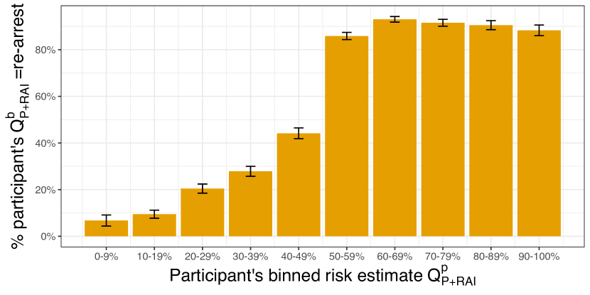
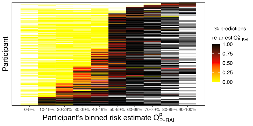
Figure 3. Comparison of risk estimates $Q_{P+RAI}^{p}$ and corresponding binary predictions $Q_{P+RAI}^{b}$ made by participants in presence of the RAI. (left) Share of assessments with predictions of re-arrest as a function of the (binned) risk estimates. Error bars represent 95% confidence intervals. For example, participants predicted that the offender would be rearrested in more than 40% of the assessments in which they estimated the probability of re-arrest to be between 40% and 49%. (right) Share of assessments with predictions of re-arrest as a function of the risk estimate and the participant. Each row corresponds to a different participant. A large fraction of the participants often—but not always—predicted re-arrests while assigning likelihoods well below 50%. Note that participants rarely applied a consistent probability threshold in predicting re-arrest.

4.1. Divergence between risk estimates and binary predictions

In §3.2, we described how the payment scheme in the second part of the survey was designed to incentivize participants to report their most accurate likelihood estimates and binary predictions. If participants adopted the profit-maximizing strategy, they would convert their likelihood estimates $(Q_{P+RAI}^{p})$ into binary predictions $(Q_{P+RAI}^{b})$ by predicting re-arrest for all those offenders for whom the value of $Q_{P+RAI}^{p}$ was 50% or greater. Only a small fraction of the participants showed this behavior. Figure 3 shows that participants assisted by the RAI predicted re-arrest even when their risk estimates were well below the 50% threshold. Approximately one fourth of the offenders (26%, se=0.5%) whose estimated probability of re-arrest was below 50% had predictions of re-arrest. Conversely, one tenth of the offenders (9.1%, se=0.4%) whose estimated risk was larger than 50% had predictions of no re-arrest. The left panel of Figure 3 describes this phenomenon by displaying the share of predicted re-arrests (i.e., mean of $Q_{P+RAI}^{b}$) as a function of the corresponding estimated likelihood of re-arrest ($Q_{P+RAI}^{p}$), appropriately binned. We observe a gradual increment in the share of predicted re-arrests as the risk estimates increase. As one could expect, the share of predicted re-arrests drastically increases around 50%: A binary prediction is twice as likely to correspond to re-arrest if the likelihood is just above the optimal threshold (mean $Q_{P+RAI}^{b}$=44.1% for $Q_{P+RAI}^{p}\in[40\%,49\%]$, 76.4% for $Q_{P+RAI}^{p}=50\%$, 90.8% for $Q_{P+RAI}^{p}\in[51\%,60\%]$; all $p_{TT}<\alpha/3$).

The right panel of Figure 3 shows the significant heterogeneity in the strategies adopted by the participants. Approximately one third of them (32.4%, 172 out of 531) always predicted re-arrest when their probability estimate was greater than 50% and no re-arrest when their estimate was less than 50%. Approximately half of the participants (56.1%, 298) followed this strategy in at least 90% of their predictions. Interestingly, Figure 3 shows that participants did not even use fixed thresholds, i.e., for most participants there was no given threshold $t$ for which $Q^{b}=$rearrest whenever $Q^{p}\geq t$.

Consequences for evaluations of participants’ predictive performance

As discussed in §2, the results of Jung et al. (2020) were obtained by soliciting only likelihood estimates and converting them into binary predictions by applying a uniform threshold (50%) across all participants. Our findings indicate that this assumed correspondence is not borne out in practice, and analyses based on this assumption can lead to incorrect conclusions. For example, consider the question of assessing the predictive performance of our study participants’ binary predictions with converted binary predictions (obtained by thresholding $Q^{p}$ at 50%) compared to actual binary predictions $Q^{b}$. While the overall accuracy of the converted predictions is similar to that of the actual binary predictions ($59.2$% and $57.6$% resp., $p_{TT}>\alpha$), other performance metrics are quite different. The false positive rate is 8.4% lower for the converted binary predictions compared to the actual binary predictions (40.8% vs. 49.2% , $p_{TT}<\alpha$), and, instead, the false negative rate is 8% higher (40.4% vs. 32%, $p_{TT}<\alpha$).

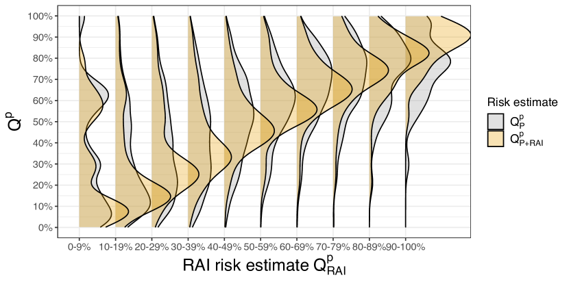
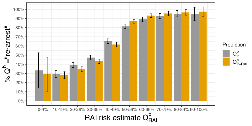
Figure 4. Analysis of predictions made by participants assigned to the non-anchoring setting in the second part of the survey. The two figures show the distribution of the pre-registered $Q_{P}$ and revised $Q_{P+RAI}$ predictions made by participants (vertical axis), grouped by the RAI’s risk estimate $Q^{p}_{RAI}$ binned (horizontal axis). (left) Density estimates of the participants’ risk estimates $Q^{p}$. Compared to the pre-registered predictions, the densities of the revised risk estimates put more mass on the interval where also the RAI’s predictions lie. This indicates that, unsurprisingly, the participants’ revised estimates were closer to the RAI’s. (right) Share of assessments with predictions of re-arrest in participants’ pre-registered $Q^{b}_{P}$ and revised $Q^{b}_{P+RAI}$ binary predictions. Error bars represent 95% confidence intervals. The agreement between the RAI’s and the participants’ predictions increased after the RAI’s prediction was shown, but the disagreement remained high in some of the buckets, even for low values of the RAI’s risk estimates.

Consequences for evaluations of participants’ reliance on the RAI

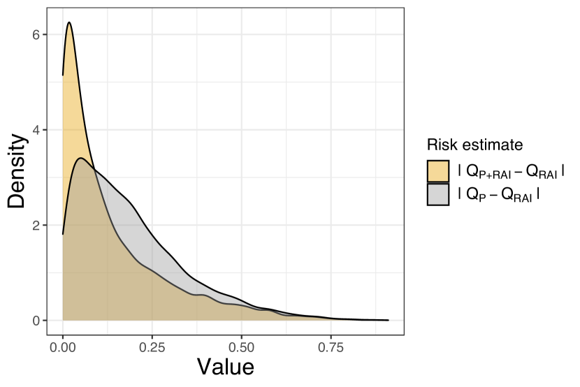
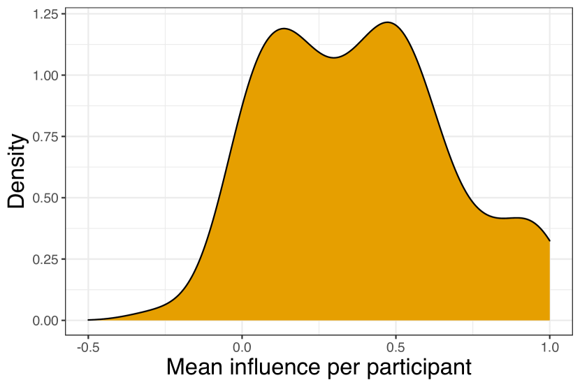
Figure 10. Analysis of risk estimates in the second part of the survey for the participants that were assigned the non-anchoring setting. (left) Kernel density estimate of the absolute differences of the participants’ initial and revised risk estimates from the RAI’s ($|Q_{P}-Q_{RAI}|$ and $|Q_{P+RAI}-Q_{RAI}|$ respectively). The figure shows that participants tended to update their estimates in the direction of the RAI’s. (right) Kernel density estimates of the mean influence of the RAI on the risk estimates by participant. We observe that participants’ revised estimates were on average closer to their initial predictions than to the RAI’s.

We now examine how participants assigned to the non-anchoring setting updated their pre-registered probability and binary predictions after they were shown the RAI. When it came to risk estimates, Figure 4 shows that participants tended to update their estimates in the direction of the RAI’s recommendation. These revisions were often substantial (mean influence=37%, see also Figure 10; in addition mean of $|Q^{p}_{RAI}-Q^{p}_{P}|=18.8\%$ vs. $|Q^{p}_{RAI}-Q^{p}_{P+RAI}|=13.3\%$). Participants changed their pre-registered binary answers in 10.2% (se=0.3%) of all predictions, switching in slightly more than half of these cases from a prediction of re-arrest to a prediction of no re-arrest (see breakdown by RAI’s score in Figure 4). However, the overall agreement with the RAI’s (binary) predictions only increased by less than 4% from the pre-registered to the revised answers (mean $Q^{b}_{P}=Q^{b}_{RAI}$:$61.7\%$, mean $Q^{b}_{P+RAI}=Q^{b}_{RAI}$:$65.4\%$, $p_{TT}<\alpha$) because participants’ final prediction often did not match the RAI’s even if their pre-registered prediction did. It is certainly possible that, had participants been provided also with the RAI’s binary predictions, we would not have observed such a phenomenon (c.f. “result 2” in Grgić-Hlača et al. (2019)). We also asked participants to self report for what share of the assessments they had revised their own predictions after taking into account the RAI’s recommendation. Interestingly, they indicated that they had revised their risk estimates and binary predictions in 59% and 34% of the assessments respectively (medians=60% and 20%). Thus, evaluations based solely on one of the two types of predictions could lead to drastically different conclusions regarding participants’ (especially self-reported) reliance on the RAI.

4.2. Absence of anchoring effects

In the introduction, we hypothesized that the participants could anchor on the RAI’s predictions. If this had happened, then the risk estimates of the participants assigned to the anchoring setting would have been closer to the RAI’s than those made by the participants assigned to the non-anchoring setting. As we might expect, we found that the pre-registered risk estimates of the participants in the non-anchoring setting were 16% further from the RAI’s than those of the participants in the anchoring setting. Yet, very surprisingly, the revised risk estimates made in the non-anchoring setting were 17% closer to the RAI’s than those made in the anchoring setting (mean and median absolute diff. $|Q^{p}_{P+RAI}-Q^{p}_{RAI}|$ in the non-anchoring setting: 13.3% and 8% resp., in the anchoring setting=16.1% and 11% resp.; $p_{MW}<\alpha$). In contrast, participants’ binary predictions matched the RAI’s at exactly the same rate across the two settings (mean $Q^{b}_{RAI}\neq Q^{b}_{P+RAI}:34.6\%$ in both). We also found that performance did not differ across the two settings: accuracy (acc. in anchoring=57.4% and in non-anchoring=57.6%), false positive rate, false negative rate, positive predicted values, and the AUC were not significantly different ($p_{TT}>\alpha$ for all comparisons).

In the perception questions, participants self reported similar levels of trust in the tool across the two settings (76.5% and 79.3% of participants in anchoring and non-anchoring resp.; $p_{TT}>\alpha$), and also of confidence and accuracy of their own predictions. Participants reported revising their binary predictions after accounting for the RAI’s at approximately the same rate in the two settings (mean reported revision=31.8% in anchoring and 33.7% in non-anchoring; $p_{MW}>\alpha$). However, the story is different in case of risk estimates. Participants assigned the non-anchoring setting self reported that they had revised their answers on average 65% more often than those in the anchoring setting after looking at the RAI’s recommendation (mean reported revision=58.9% in non anchoring, 35.7% in anchoring; $p_{MW}<\alpha$). Despite the risk estimates of the participants assigned to the non-anchoring setting were only slightly closer to the RAI’s, their perceived use of the tool to adjust risk was substantially higher. It seems possible that, by pre-registering their risk estimates, participants became more aware of the influence of the RAI on their risk estimates.

To summarise, we did not find evidence of anchoring effects. Instead, we found the opposite: The predictions made by participants in the non-anchoring setting were closer (in absolute distance) to the RAI’s. These participants also self-reported that the tool had influenced more heavily their risk estimates.

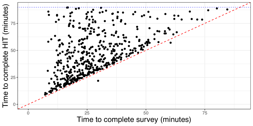
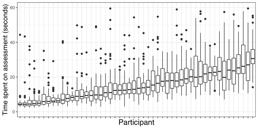
Figure 5. Analysis of time. (left) Time taken to complete the HIT on Mechanical Turk (vertical axis) as a function of the time spent on the survey (horizontal axis) for each participant. The blue dotted line corresponds to 90 minutes, which was the maximum time allowed on Mechanical Turk for the submission of the HIT. Each black dot corresponds to an individual participant. The observations below the diagonal line correspond to participants that started the survey before accepting the HIT. If the time on Mechanical Turk and on the survey were similar for each of the participants, the observations would lie close to the dashed red line at 45 degrees. We observe that the time taken to complete the HIT was generally substantially larger than the time spent on the survey. (right) Boxplot of the time spent on each offender’s assessment by every participant. The whiskers extend from the hinges to the smallest or largest values at most 1.5$\cdot$IQR of the hinge. For visualization purposes we randomly sampled 100 participants from those that had been assigned to the anchoring setting and limited the length of the vertical axis.

4.3. Time spent on the survey as a poor proxy for time spent on the assessment

Participants completed all the steps in the survey, from login to submission, in an average time of 28 minutes (sd=13.5). In comparison, the average time recorded on Mechanical Turk, from the acceptance to the submission of the HIT, was 68% greater, averaging 46.7 minutes (sd=20.2). The left panel of Figure 5 shows the time spent on the survey and on Mechanical Turk for each participant. The time spent on the survey was on average 89% greater than the time recorded on the platform. For 27.9% of the participants (139 out of 499) the submission of the HIT took 5 minutes less than the completion of the survey; for 43.5% of them (217) it took 10 minutes less, and for 63.1% of them (315) it took 20 minutes less. Figure 5 also reveals that the time spent on the survey varied considerably across participants, from less than 10 minutes up to more than one hour. An analysis at a more granular level reveals that the assessment of an individual vignette was carried out on average in 15 seconds (sd=34.2, median=10). Once we excluded the pre-registered and revised predictions made by the participants assigned to the non-anchoring setting in the second part of the survey, the average time was $17.5$ seconds (sd=39.2, median=12.2).

The substantial difference between the mean and the median raises the following question: Is the time taken to complete the survey (divided by the number of questions) a reliable proxy for the time spent on each question? Equivalently, do participants spend the same amount of time on all question? The right panel of Figure 5 shows that participants generally did not allocate their time equally across questions. On average, they spent more than one tenth of their time on the assessment of only one offender (out of 40, mean proportion of time per participant=12.1% and median=7.7%) and one fifth of their time on four assessments (20.3%, median=16.6%). Once the four assessments that took longest were removed for each participant, the time spent that each of them spent on the assessments decreased on average by 19.4%. We also found, as might be expected, that participants tended to spend more time on the first question of each part of the survey. For example, in the first part of the survey, participants spent on average almost 9 seconds more on the first question than in the others (average time first question=26.8 and median=17.6 seconds, others mean=17.9 and median=12.4; $p_{MW}<\alpha$). Similarly, the first question in the second part of the survey took twice as much time as the others (average time first question=30.6 seconds, others=17.2; $p_{MW}<\alpha$). We could not identify any other clear reasons for why some predictions took longer than others. It is likely that participants simply took breaks from the survey. Nonetheless, they allocated the time proportionally to the number of questions in each of the two parts of the survey (i.e., on average 37.8% of their time on the first part of the survey that contained 35%=14/40 of the offenders).

We also examined whether time was related to predictive performance. For the participants that had been assigned to the anchoring setting, the time spent on the entire survey was weakly correlated with the accuracy of the binary predictions ($\rho_{S}=0.3$, $p<\alpha$). However, we observe that this correlation is mainly due to the participants that completed the surveys very quickly and also achieved very low accuracy. Assessments on which predictions were accurate did not take longer than inaccurate predictions on average ($p_{TT}>\alpha$) and only the median time was slightly higher (median time accurate=12.4 seconds and inaccurate=11.9; $p_{MW}<\alpha)$. Given the large variance in the time spent on the assessments across participants, we also tested a similar hypothesis. For each participant, we ranked their 40 predictions in increasing order of time. The mean ranking of the predictions that were accurate was, perhaps unexpectedly, lower than that of the those that were inaccurate. One possible explanation is that some vignettes are easy to get right, and thus do not require much time to complete.

In summary, we found that the time taken to complete the HIT on Mechanical Turk was a severe overestimation of the time that participants spent on the survey. The time spent of the survey was also a poor proxy for the time spent on each vignette, given that participants typically spent a substantial share of their time on only a few assessments. Lastly, we found little evidence of any association between time spent by the participants on the assessment and accuracy of their predictions.

4.4. Predictions are not decisions

In our study, participants were asked to provide likelihood estimates and binary predictions of offenders’ re-arrest outcomes. As we discuss in this section, our findings concerning how humans update their predictions when presented with the RAI’s recommendations—and findings from these types of studies more generally—do not readily translate into implications for decision-making. Firstly, there is the clear issue that our study participants are not judges, and are not being presented with the full set of information that judges would have access to in real world decision-making settings. However, we would not be surprised if conducting our experiment on a population of judges produced largely the same qualitative findings regarding risk predictions. The bigger issue that we wish to draw attention to here is that risk is just one of many factors that judges are asked to consider in their decisions.

In the context of sentencing, considerations of risk are often secondary to factors such as the severity of the offense and restitution to victims. The offender’s risk of re-arrest often enters into decisions indirectly through considerations of prior criminal history, which is a leading predictor of future recidivism. For instance, the Pennsylvania Commission on Sentencing has adopted a set of sentencing guidelines that “provide sanctions proportionate to the severity of the crime and the severity of the offender’s prior conviction record” (Pennsylvania Commission on Sentencing, 2020). These guidelines are primarily a function of two factors: the offense gravity score (OGS), which is a measure of the gravity of the most serious crime among the offender’s current charges; and the prior record score (PRS), which is a composite measure summarizing prior criminal records. Higher values of OGS and PRS correspond to more serious offenses and more severe prior criminal histories (Hyatt and Chanenson, 2016). While the recommendations are advisory, judges need to provide a written justification when their sentencing decisions deviate from the recommended range.

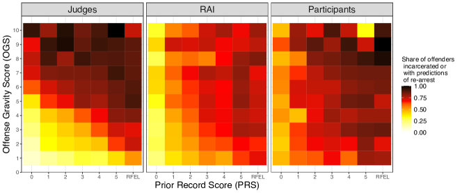
Figure 6. Comparison of judicial decisions of incarceration, binary predictions of the RAI, and binary predictions of participants (both $Q_{P}$ and $Q_{P+RAI}$). The threshold for converting the RAI’s risk estimates into binary predictions for this analysis was set such that the overall share of predicted re-arrests was equal to the incarceration rate. The color in each cell is proportional to the share of offenders that were incarcerated (judge) or with predictions of re-arrest (RAI and participants), for specific values of the offense gravity score (OGS) and prior record score (PRS). In this figure, the heatmaps for judicial decisions and RAI’s predictions were generated using all offenders in the test set.

Our data contain information not only on re-arrest outcomes, but also on judicial sentencing decisions. This allows us to compare judicial decisions of whether to sentence the offender to a period of incarceration to the predictions of re-arrest made by participants and RAI. Figure 6 shows judicial decisions along with participants’ and RAI’s predictions broken down by levels of the OGS and the PRS. For judges, we observe that the likelihood of incarceration increases with both the PRS and OGS. But the pattern is more complex in case of participants’ and RAI’s predictions of re-arrest: The likelihood of a predicted re-arrest appears to increase with the PRS, but it does not seem to be associated with the OGS.

We investigated how the likelihood of incarceration and the predictions of re-arrest made by participants and RAI depended on the PRS and the OGS by fitting three separate logistic regression models of the form $outcome\sim PRS+OGS$. We treated both scores as numeric (repeated felony offender, “RFEL”, was converted into a score of 6) and set the threshold for the RAI such that the share of predicted positives was equal to the share of offenders that were incarcerated. The coefficients of the OGS were $0.05$, $0.08$, and $0.49$ for the models targeting predicted re-arrest by participants, by the RAI, and incarceration respectively (all $p<\alpha$). These results would indicate that, ceteris paribus, an increase in the OGS by one level was associated to a 63% increase in the odds ratio of the likelihood of incarceration but only to a 5% increase in that of the participants’ predictions of re-arrest (see the full results in Table 4).

To take a concrete example, consider the subgroup of offenders charged with drug offenses. Among these offenders, 68% of those charged with felonies were incarcerated, compared to only 21% in case of misdemeanors. Yet, the rate of re-arrest was virtually identical across the two types of charges (47% and 45% respectively). In comparison, participants and the RAI, once equalized for overall rates, predicted re-arrest for only a slightly higher share of the felony offenders (share of predictions of re-arrest for felonies: RAI=43% and participants=66%; misdemeanors: RAI=52% and participants=59%). This indicates that there are cases where differences in decisions are unrelated to the risk of recidivism (here, the decision of whether to incarcerate).

Because risk predictions are not aligned with the OGS, and the OGS is one of the primary determinants of criminal sentences, we should not expect findings of how judges’ predictions change when provided with RAI information to be directly informative of likely changes in the resulting decisions. Even if our findings that participants revised their risk predictions when presented with the RAI’s recommendation generalized to judges, it is unclear what effect, if any, those revised assessments would have on sentencing outcomes.

5. General discussion

5.1. Limitations

There are several limitations related to the generalizability of our results. First, despite our strict exclusion criteria, the analysis in §4.3 revealed that a substantial share of the assessments were carried out very quickly, often in less than 5 seconds. This indicates that participants often did not fully read the offenders’ descriptions or did not think carefully about their answers. The post-hoc analyses, however, have revealed that our conclusions were largely unaffected by the presence of these predictions in the data. It is also unclear whether our findings would generalize to other experimental setups (such as those with different incentive structures), populations of participants, domains, or to real-world decision-making settings. For example, we might expect judges to exhibit many of the cognitive biases exhibited by our survey participants (Guthrie et al., 2000) and suspect they might also overestimate their own predictive abilities (DeMichele et al., 2018b), which may result in lesser reliance on the RAI. Consequently, the impact of the RAI on their judgment may be different than what has been observed in our experiment. Another potential limitation is that our results could have been affected by our explanations of the incentive structure, information regarding the RAI, and framing of the questions. We also note that our pool was composed of Amazon Mechanical Turk workers that were $20$–$40$ years old, a demographic group that is likely tech-savvy and more open to the introduction of technologies than other populations (Redmiles et al., 2019). As such, it is not a representative sample of the broader US population, and is not demographically representative of the US judiciary. Lastly, it is possible that, due to the negative experiences that workers often have on Mechanical Turk (Fort et al., 2011; Mason and Suri, 2012), running the experiment on an alternative platform could lead to different results, especially those discussed in §4.3.

5.2. Discussion

In our study, participants often predicted re-arrest even when assigning a low numeric score to the likelihood of that event. We offer four hypotheses that could explain this behavior. The first is poor numeracy skills: Even highly educated individuals tend to struggle with simple numeracy questions (Black et al., 1995; Schwartz et al., 1997; Lipkus et al., 2001; Visschers et al., 2009). Some of our participants may have not realized that the expected profit-maximizing strategy is to predict that the given offender would be re-arrested if and only if they believed the risk of rearrest is greater than 50%. A second explanation might be that participants’ subjective likelihood judgments did not simply reflect the estimated frequencies of events (Manski, 2004; Evans et al., 2004), e.g., due to an asymmetry in the perceived cost of errors. This hypothesis seems plausible, even though participants were incentivized through the payment scheme to report calibrated probability estimates. A third explanation might be lack of care: We found that, while the observed phenomenon held in general, it was more common among the predictions that took the least time. Consequently, it is possible that some of the participants made the predictions quickly and without paying adequate attention, e.g., satisficing. The fourth explanation might be that participants did not understand the slider instrument, despite being provided with a clear set of instructions (see §C.3). However, given that this instrument is prevalent in current practice (Roster et al., 2015) and it generally has high concurrent validity with respect to other types of instruments such as Likert scales and radio buttons (Couper, 2008), this hypothesis seems unlikely to explain our results. Future work might explore why this phenomenon occurred.

It is of paramount importance to employ measures that are comprehensible to the human and can also be effectively and consistently estimated by the human. It is also equally important that the RAI’s recommendations be easily understood by the human. Different ways to communicate the RAI’s prediction can help decision makers calibrate their trust in the RAI (Zhang et al., 2020; Lai and Tan, 2019) and, potentially, also reduce variability in their decisions. The comparison between our results around how people often switch their (binary) predictions not in the direction of the RAI’s and the findings in Grgić-Hlača et al. (2019) likely represents an example of the importance of such design choices. Another notable implication of this result is that the type of prediction on which participants’ predictive performance and reliance on the RAI’s recommendations are evaluated can affect the conclusions that researchers draw from the study. In our experiment, for example, an analysis that focused only on binary predictions would have neglected the role of the RAI in influencing participants’ risk estimates. While the choice of the type of prediction might be context-dependent, the potential limitations of the assessment should be recognized and acknowledged.

One notable and unexpected finding in our work is the absence of anchoring effects. We designed the second part of the survey to determine how much (if at all) participants anchored on the RAI’s predictions. For binary predictions, we found no difference in the agreement between the participants and the RAI across the two settings. For risk estimates, not only did our participants not anchor on the RAI—participants who were shown the RAI directly gave predictions further from the RAI’s than participants that had pre-registered their estimates before seeing the RAI’s outputs. One possible explanation of this behavior is that participants felt that they had to—or wanted to—demonstrate a sense of agency. According to this hypothesis, participants assigned to the non-anchoring setting, who had already delivered risk estimates without the assistance of the RAI, would have been more comfortable with accepting the RAI’s predictions, having already demonstrated their agency. At the same time, participants assigned to the anchoring setting might have felt compelled to offer predictions that differed from those of the RAI to demonstrate that they were performing the task earnestly and not simply copying the RAI. Another possible explanation for this phenomenon might be that the users who pre-registered their predictions also had the opportunity to notice how similar the RAI’s predictions were to theirs and might consequently have trusted the RAI more. However, these users did not report higher levels of trust in the tool. Yet they reported making a heavier use of the tool’s predictions. This finding opens an interesting new direction for future research: If these results held in other experiments, could we improve experts’ perceived and actual reliance on algorithmic tools by eliciting predictions from the experts both before and after revealing the RAI’s recommendation?

Like past works, we found that even when participants were shown the RAI’s predictions, they continued to underperform the RAI in terms of predictive accuracy. It seems possible that this observation may characterize many forecasting settings where both the RAI and humans have low accuracy. Tan et al. (2018) demonstrated that even if the predictions made by the RAI and the human alone were combined, the resulting unavoidable error may still be very large. We note that in our experimental setting we would not expect participants’ predictions to outperform those of the RAI. This is because the RAI has access to all of the features that participants are able to consider, and is trained to optimize for predictive accuracy. In practice, judges have access to information that the tool does not. Further studies of human-in-the-loop systems are needed to examine the influence of the overlap in information sets between humans and the RAI on predictive performance, participants’ trust in the tool, and decision-making. It is likely that even in the case of complementary information sets, or where participants have access to more information than is available to the tool, it will be difficult for humans to match the RAI’s performance without carefully crafted feedback.

Unsurprisingly, the time that participants actually spent on the survey was substantially lower than the time taken to submit the HIT and did not even represent a reliable proxy for the time spent on the assessment of a single vignette. In addition, participants who spent more time on the survey did not, in general, achieve higher predictive accuracy. Ideally, especially in tasks characterized by high degrees of uncertainty such as the prediction of criminal recidivism, researchers might want to design compensation structures in which the assigned reward is proportional to the effort made by the participant. While time itself is not a perfect measure of effort, future work could employ exclusion criteria based on the time that participants spend on each assessment. Time spent is also worth taking into account when assessing the generalizability of study findings, especially with respect to real-world decision-making in high-stakes settings. For example, researchers could run post-hoc analyses to assess whether their conclusions still hold once the predictions that participants made quickly are dropped. In our experiment, as we already mentioned, the main results still held even when these predictions were not considered in the analysis.

Lastly, in §4.4 we showed that, unlike judicial decisions, the predictions made by participants were weakly associated to the seriousness of the offender’s current charge. For drug felonies and misdemeanors, predictions were nearly orthogonal to the gravity of the offense. This finding sheds light on the limits of the use of human predictions of criminal recidivism as proxies for judicial decision-making: Even if studies found large effects of the impact of RAI’s recommendation on human predictions (which they have not), further investigation would be required to understand how or whether those would translate to decisions. Such an analysis would not only require understanding for which offenders decisions and predictions would diverge, but also how the introduction of the RAI would reshape the existing decision-making framework. For example, in the Pennsylvania sentencing system, the newly adopted RAI is used to determine when a pre-sentencing investigation report is to be generated, which would provide judges with additional information on the offender (on Sentencing, 2020a). In the New Jersey pretrial system, the RAI represents a building block of the decision-making framework, but it is not its only element (Courts, 2018). There, the RAI is also used to decide whether a summons or a warrant should be issued. Thus, the RAI potentially affects not one but many sequential decisions made at several stages of the pipeline by interacting with other elements in a larger framework.

6. Acknowledgments

We are grateful to PwC USA for funding this research through the Digital Transformation and Innovation Center sponsored by PwC. We also deeply thank Shamindra Shrotriya and Pratik Patil for providing valuable feedback on the survey.

Appendix A Additional details on methodology

Assessing the candidate RAIs for racial predictive bias

One of the questions we sought to answer with our study is whether the extent or manner in which participants responded to RAI’s predictions showed indications of racial bias as previously found in Green and Chen (2019a) and Green and Chen (2019b). To ensure that our results would not be confounded by the use of an RAI that itself systematically over or underestimates the likelihood of re-arrest for certain racial groups, we performed a group-level calibration analysis of all four models being considered for use in the experiment.

We first assessed the model’s racial calibration properties via logistic regression following the approach of Skeem and Lowenkamp (2016). This entails a comparison of the relative fit of the following three nested logistic regression models: $Y\sim\text{score}$, $Y\sim\text{score}+\text{race}$ for “intercept bias”, and $Y\sim\text{score}+\text{race}+\text{score}\times\text{race}$ for “slope bias” through a likelihood ratio test or a Wald test for the coefficient of the added variable, where $Y$ indicates the re-arrest (Y=1 if re-arrest occurs, 0 otherwise). None of the models showed intercept bias (all $p>\alpha$) and only XGBoost presented slope bias (all others $p>\alpha$). Due to the likely misspecification of the logistic regression model adopted in the test, we additionally relied on the chi-squared test of Fogliato et al. (2020). We separated the RAI’s predictions by offenders’ racial groups and divided them into bins of width $0.1$ ($[0,0.1),[0.1,0.2),\dots,[0.9,1]$). The test revealed an overestimation of the risk for White offenders (compared to Black offenders) in the logistic regression and XGBoost models for the predictions in the bins $[0.3,0.4)$ and $[0.7,0.8)$ respectively.

We then examined the models for error rate balance. All four models showed false positive rates on Black offenders that were more than twice as large as those on White offenders (around 35% and 13% respectively), but also lower false negative rates for Black offenders (around 35% and 67% respectively). This is expected in settings where the outcome base rates differ across groups, as is the case in the present study. Positive predictive values were higher for Black offenders (around 66% vs. 60%). All differences were statistically significant (all $p<\alpha$). Lastly, we checked whether the models produced similar AUCs across racial groups, a criterion named accuracy equity (Dieterich et al., 2016). The AUC of the predictions on Black offenders was slightly higher than the AUC of those on Whites across all models (around $70\%-71\%$ and $68\%-69\%$ respectively).

Appendix B Additional results

This section is organized as follows. In §B.1 we compare participants’ and RAI’s predictive performances. In particular, we show that participants always underperformed the RAI. In §B.2 we show that, similarly to the results of Green and Chen (2019a), participants’ self-reported predictive accuracy was correlated with their real accuracy only when outcome feedback was provided. In §B.3 we show that, in contrast with past work (Green and Chen, 2019a, b), we did not find evidence of disparate-interactions in the participants’ uptake of the RAI’s predictions. However, their risk estimates overestimated the risk of re-arrest for Whites compared to Blacks and their binary predictions produced higher false positive rates for Blacks. In §B.4 we show that the order in which the offenders’ profiles were shown did not affect participants’ trust and reliance on the RAI. Lastly, in §B.5 we extend the results around the impact of the RAI on participants’ predictions presented in §4.1.

B.1. Evaluation of predictive performance: Participants performed worse than the RAI according to all metrics other than the false negative rate

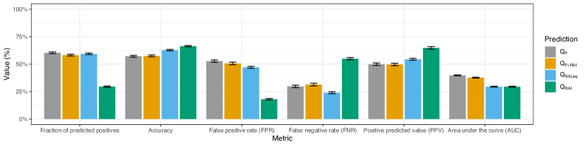
Figure 7. Performance metrics relative to the predictions made by participants alone ($Q_{P}$), participants assisted by the RAI ($Q_{P+RAI}$), and by the RAI alone with risk estimates converted into binary predictions using the threshold of 50% ($Q_{RAI}$) and another for which the fraction of predicted positives was equal to the participants’ ($Q_{RAI,eq}$). The metrics considered are fraction of predicted re-arrests, accuracy, false positive rate (FPR), false negative rate (FNR), positive predicted vaues (PPV), and area under the curve (AUC). The first five metrics are based on the binary answers given by the participants ($Q^{b}$), whereas the AUC is based on the risk estimates ($Q^{p}$). Error bars indicate 95% confidence intervals.

In this section we analyze the predictive performance of the predictions made by our study participants, both with and without the RAI, across a range of different metrics. Binary classification metrics such as accuracy and false positive rates were computed based on participants’ responses to the binary prediction question $Q^{b}$. Area under the curve calculations are based on participants’ probability predictions $Q^{p}$. For this analysis, $Q_{P}$ includes all answers made by participants in absence of the RAI both in the first and second parts of the survey.

One challenge in comparing the binary classification performance of the RAI to participants’ predictions is that the fraction of cases for which the RAI’s predicted probabilities exceed $0.5$ is very different from the fraction of cases in which participants predicted re-arrest. To make the participants’ and RAI’s predictions comparable, we obtained additional binary predictions from the RAI’s risk estimates using a threshold for which the fraction of predicted positives for the RAI was equal to the participants’. This is denoted by $Q_{RAI,eq}$ in the results.

Figure 7 summarizes our findings. We observe substantial differences between the RAI’s and the participants’ metrics. On average, the RAI outperformed their predictions across all metrics considered other than the false negative rate, while the rate-equalized RAI outperformed their predictions on all metrics including the false negative rate. There is no notable difference in the metrics between the predictions that were made by participants alone and those in presence of the RAI, thus we only focus on the latter.

Participant predicted re-arrest in twice as many assessments as the RAI did (mean for $Q_{P+RAI}$=58.2% and for $Q_{RAI}=29.5\%$; $p_{TT}<\alpha$). The accuracy of their predictions was 8.8% lower than the RAI’s (acc. for $Q_{P+RAI}=57.5\%$ and $Q_{RAI}$=66.3%; $p_{TT}<\alpha$). The false positive rate of their predictions was three times higher than the RAI’s, but only slightly higher than that of the rate-equalized RAI (FPR for $Q_{P+RAI}=50.6\%$, $Q_{RAI,eq}=47\%$, $Q_{RAI}=18\%$; all $p_{TT}<\alpha$). In contrast, the predictions of the RAI presented higher false negative rates than the participants’ and the RAI with equalized rate’s (FNR for $Q_{P+RAI}=31.4\%$, $Q_{RAI,eq}=23.9\%$, $Q_{RAI}=54.9\%$; all $p_{TT}<\alpha$). The positive predicted values of the RAI and RAI with equalized rate were 31% and 9% higher than the participants’ (PPV for $Q_{P+RAI}=49.7\%$, $Q_{RAI,eq}=54.4\%$, $Q_{RAI}=64.8\%$; all $p_{TT}<\alpha$). The area under the curve produced by the RAI’s risk estimates was 13% higher than the participants’ (AUC for $Q_{P+RAI}=62\%$, $Q_{RAI}=70.1\%$).

When we looked at the performance of individual participants instead of averaging over all participants, we did find evidence of human performance, in some cases, exceeding that of the RAI. In the second part of the survey, 31% of the participants had an accuracy higher than the RAI’s. Thus, while most participants were unable to improve upon or match the predictive performance of the RAI even when presented with the RAI predictions, some did.

Past work has noted that participants’ accuracy, in presence of feedback, slowly increased with the number of examples that were shown (Jung et al., 2020). In our study, participants received feedback on only the first 14 assessments (compared to 50 in past work), but they could still learn by seeing the RAI’s predictions. We did not find evidence of any increase in accuracy throughout the survey. The accuracy of participants remained stable across the assessments in the first part of the survey (accuracy first 7 offenders=57.7%, second 7 offenders=57.3%) and was not higher for the pre-registered predictions.

B.2. Evaluation of predictive performance: Participants’ self-reported predictive accuracy was correlated with actual accuracy only in presence of feedback

In the perception questions, we assessed whether participants could correctly guess their own accuracy and the confidence in their predictions (see all questions in §C.8). In the question regarding accuracy, participants were asked what share of their binary predictions they thought were accurate. In the first part of the survey, where participants were provided with outcome feedback after each vignette, participants’ perceived accuracy was strongly positively associated to their real accuracy ($\rho_{S}=0.49$; $p<\alpha$). When feedback was removed in the second part of the survey, participants were unable to correctly guess their own accuracy: The self-reported accuracy was uncorrelated with their actual performance ($\rho_{S}=-0.05$; $p>\alpha$). In the second part of the survey, the average perceived performance was substantially larger than the real performance (perceived=59.8% vs. real=57.5% in first part, perceived=65.7% vs. real=57.5% in second part). 42% of participants overestimated their own accuracy in the first part of the survey, compared to 58% in the second part.

When asked about confidence in their own predictions, the participants that reported higher levels of perceived accuracy were also more confident in their own predictions (in the first part the mean self-reported accuracy of participants that were confident=66.2%, neutral=58%, and not confident=46.2%; all $p_{MW}<\alpha$. Similar results were found for the second part). There was a slight increase in the confidence levels of the participants between the first and second part of the survey, with just 12.4% reporting that they were ‘not confident’ in their predictions in the second part, compared to 19.6% in the first part. Overall, we found that throughout the survey participants became more optimistic about their accuracy and slightly more confident in their own predictions, potentially due to the absence of feedback.

We also asked participants to evaluate the accuracy of their own predictions compared to those of other participants. More than half of the participants thought that their own accuracy was approximately equal to the median accuracy (54.4% and 55% in the first and second parts of the survey respectively). A large share of participants deemed their own performance to be higher than the median accuracy and this share increased from the first to the second part if the survey (30.3% and 37.5% of participants in first and second parts respectively). When feedback was given, their evaluations were associated to the real ranking ($p_{MW}>\alpha$ for the comparison of substantially higher than median vs. around the median, $p_{MW}<\alpha$ for the others). In the second part of the survey, where feedback was removed, perceived ranking was no longer significantly associated to real ranking (all $p_{MW}>\alpha$).

B.3. Racial disparities in predictions

In this section we investigate whether the predictions that participants made in presence of the RAI suffered from predictive bias and could lead to disparate impact. We found that these predictions presented higher false positive rates on Black offenders, but more severely overestimated the risk for White offenders compared to Blacks. In contrast to Green and Chen (2019a), we found no evidence of racial bias in the uptake of RAI’s predictions. As a reminder, in §A we show that the RAI’s predictions presented higher false positive rates on Black offenders and produced a lower area under the curve for Whites, but passed the calibration tests.

Participants largely overestimated the share of re-arrests for both racial groups (predictions of re-arrests=70% and 51.8% for Black and White offenders respectively). They performed slightly better on the Black population of offenders in terms of accuracy and area under the curve (accuracy for Whites=$56.3\%$ and for Blacks=$59.7\%$, $p_{TT}<\alpha$; AUC for Whites=$60.3\%$ with 95% confidence interval $[59.3\%,61.3]$ and for Blacks=$62.4\%$ and 95% confidence interval $[61.7\%,63.2\%]$). The other metrics presented substantial differences across the two racial groups. The false positive rate on Black offenders was higher by 14% compared to Whites (FPR for Whites=46.5% and for Blacks=60.7%, $p_{TT}<\alpha$) but the false negative rate was lower by 18% (FNR for Whites=39% and for Blacks=21.3%, $p_{TT}<\alpha$). Positive predicted values were 58.3% for Blacks and as low as 43.5% for Whites ($p_{TT}<\alpha$). We also conducted two test of calibration (see §A for more details on these tests). Probability predictions suffered from both intercept and slope bias in the calibration test via logistic regression (coef. of White race=-0.45 and interaction=-0.54 respectively; both $p<\alpha$) (Skeem and Lowenkamp, 2016). Predictions also failed the calibration test via chi-squared ($p<\alpha$ for all $\lfloor Q_{P+RAI}\cdot 10\rfloor\geq 5$), where the share of re-arrests for Blacks was higher than for Whites across all bins.

We checked whether the RAI’s influence on the predictions of the participants depended on the offender’s racial group. We tested this hypothesis on two sets of predictions: (i) the pre-registered and revised risk estimates in the non-anchoring setting; and (ii) all risk estimates made without and with the assistance of the RAI. In (ii), we considered only those offenders that had at least 3 predictions of each type, averaged the answers, and then computed the influence. For both (i) and (ii), we found that the RAI exerted approximately the same influence across racial groups ($p_{MW}>\alpha$ for both). In contrast to the findings of Green and Chen (2019a), we found that, in cases where the risk estimates made by participants alone were lower than the RAI’s, the influence of the RAI was not larger for Black offenders neither in (i) nor in (ii) ($p_{MW}>\alpha$ for both).

B.4. The order of the offenders’ profiles did not affect participants’ interactions with the RAI

As we mentioned in §3.2, in some cases the offenders’ profiles were not randomly ordered. More specifically, the participants were assigned to one of three conditions, that we call random, controlled, and decreasing. In the ‘random’ setting, participants were shown a randomly sampled set of offenders. In the other two conditions, we sampled a set of offenders on which the RAI achieved the same accuracy as in the population (i.e., 16 or 17 out of 25 predictions were correct). In the ‘controlled’ setting participants were presented with the offenders’ profiles sorted in random order. In the ‘decreasing’ setting, participants were first shown the offenders for whom the RAI had made accurate predictions and then those for whom the RAI’s predictions were inaccurate. See Table 2 for the distribution of participants across conditions. Here we only focus on the comparison of the controlled and decreasing conditions.

We initially expected the participants assigned to the decreasing condition to exhibit more trust in the RAI and their risk estimates to be more heavily influenced by the RAI compared to those of the participants assigned to the controlled condition. We found little or no evidence of such phenomena: Our results show that, in absence of feedback, participants’ trust and reliance on the RAI were not impacted by the accuracy of its predictions on the initial set of cases.

None of the performance metrics differed across the two settings other than for the area under the curve, which was larger by almost 4% for the predictions made in the controlled condition (AUC for controlled=62.2% and 95% c.i. $[61.1\%,63.4\%]$, for decreasing=$58.6\%$ and c.i. $[57.3\%,59.8\%]$; all $p_{TT}>\alpha$ for other comparisons). The risk estimates made in the two conditions were similarly close to the RAI’s (mean $|Q^{p}_{P+RAI}-Q^{p}_{RAI}|$ for controlled=$16\%$ and for decreasing=$17.5\%$; $p_{MW}>\alpha$). In the last set of perception questions, participants self reported trusting the RAI at approximately the same rate across the two conditions (81.5% and 80.3% in controlled and decreasing respectively; $p>\alpha$). Interestingly, trust was not affected by the level of accuracy of the RAI’s predictions: Among the participants assigned to the decreasing condition, the same share of participants reported trust in the tool in the second and third sets of perception questions. We also observed no notable differences in the levels of confidence and self-reported use of the RAI across the two conditions.

	Anchoring	Non-anchoring
Random	20.2% (107)	20% (106)
Controlled	12.1% (64)	12.4% (66)
Decreasing	16.8% (89)	18.6% (99)

Table 2. Distribution of participants across the 2 settings (anchoring, non-anchoring) and the 3 conditions (random, controlled, decreasing). Raw counts are reported inside parentheses.

B.5. Participants often revised their risk estimates when provided with the RAI’s prediction, but were less likely to revise their binary predictions in the direction one would expect

In this section, we provide a longer discussion on how participants assigned to the non-anchoring setting revised their predictions after gaining access to the RAI’s. These results extend those in §4.1.

Participants’ predictive performance did not significantly improve when they were presented with the RAI’s predictions (accuracy for $Q_{P}^{b}=56.7$ vs $Q^{b}_{P+RAI}=57.6\%$, $p_{TT}>\alpha$). The main exception is in the case of AUC, for which we detect a statistically significant improvement of 2.8% (mean AUC for $Q_{P}^{p}$=60.1% and 95% conf. int. $[59.2\%,61\%]$, mean AUC for $Q^{p}_{P+RAI}=62.9\%$ and 95% conf. int. $[62\%,63.8\%]$). However, this does not mean that participants did not revise their predictions when provided with the RAI’s. This result should be expected in light of the fact that participants often revised only their risk estimates in the direction of the RAI’s.

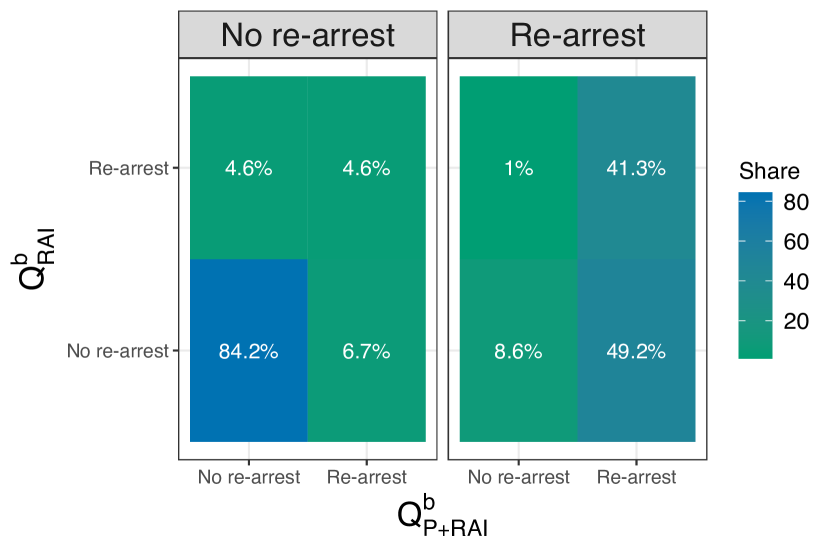
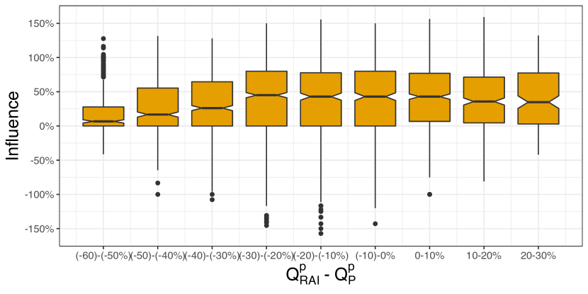
Figure 11. Analysis of binary predictions in the non-anchoring setting. (left) The heatmaps correspond to pre-registered binary predictions corresponding to no re-arrest (left) and re-arrest (right). The binary predictions of RAI and the final revised answers of participants lie on the vertical and horizontal axes respectively. The percentages correspond to the fraction of observations falling in each category. For example, the percentage in the bottom left corner indicates the share of all pre-registered predictions corresponding to no re-arrest (approximately 40% of all predictions) that matched the RAI’s (binary) prediction and that were not revised. The bottom right corner of the heatmap on the left and the top left corner of the heatmap on the right represent interesting cases of participants switched prediction even though their pre-registered answers matched the RAI’s predictions. (right) Boxplot of the influence of the RAI on participants’ risk estimates grouped by the difference between the RAI’s predictions ($Q^{p}_{RAI}$) and the participants’ pre-registered risk estimates ($Q^{p}_{P}$). The whiskers extend from the hinges to the smallest or largest values at most 1.5$\cdot$IQR of the hinge and the notches extend to 1.58$\cdot$IQR /$\sqrt{n}$. If participants were to blindly rely on the RAI and always match its predictions (i.e., a case of automation bias), most of the mass of the boxplots would lie around 100%. We observe that this does not occur. The median influence of the RAI is always below 50% and decreases as the gap between the RAI’s and the pre-registered risk estimates decreases.

As we discussed in §4.1, participants’ revised risk estimates were closer to the RAI’s than their pre-registered estimates. Interestingly, the RAI’s influence was 36% higher when the participant’s pre-registered risk estimate was lower than the RAI’s (mean inf. when $Q^{p}_{P}<Q^{p}_{RAI}:\;44.8\%$, when $Q^{p}_{P}>Q^{p}_{RAI}:\;32.9\%$; $p_{MW}<\alpha$) but the average size of the revision was lower (mean $|Q^{p}_{P+RAI}-Q^{p}_{P}|$ when $Q^{p}_{P}<Q^{p}_{RAI}:\;6.7\%$, when $Q^{p}_{P}>Q^{p}_{RAI}:\;7.9\%$). The magnitude of these revisions was not always orthogonal to the magnitude of the initial difference: Influence was uncorrelated with the difference only in case of the pre-registered probability prediction being lower than the RAI’s ($\rho_{S}=0.2$ for $Q^{p}_{P}>Q^{p}_{RAI}$ and $p<\alpha$; $\rho_{S}=-0.05$ for $Q^{p}_{P}<Q^{p}_{RAI}$ and $p>\alpha$) (see also Figure 11 in §D). The two results together indicate that the relative—but not the absolute— magnitude of participants’ revisions was larger in cases where they had initially underestimated the probability of re-arrest compared to the RAI. This could be expected given that the initial risk estimates made by participants generally were substantially higher than those of the RAI (mean $|Q^{p}_{P}-Q^{p}_{RAI}|$ when $Q^{p}_{P}>Q^{p}_{RAI}$: $21.6\%$ vs when $Q^{p}_{P}<Q^{p}_{RAI}$: $14.1\%$). Despite quite large heterogeneity in the influence of the RAI across participants (see Figure 10), we identified three notable patterns in their answers. Approximately 6% of the participants always matched the RAI’s predictions (17 out of 271), 7% never revised their risk estimates (19), and 11% always averaged their initial risk estimates with the RAI’s (29).

Participants revised their pre-registered binary predictions in 10.2% (se=0.3%) of the assessments, switching in slightly more than half of these cases from a prediction of re-arrest to one of no re-arrest (share of predictions that switch from re-arrest to no re-arrest: $5.7\%$). Here, two results are worth mentioning. First, when the participants changed their predictions, they not always did so to match the RAI’s: This occurred only in 68.3% of all revisions. In 5.2% of the cases where the participants’ pre-registered answers matched the RAI’s, their revised predictions did not. Second, the likelihood that participants would switch their prediction to match the RAI’s varied with the actual recommendation: In cases where the pre-registered prediction did not correspond to the RAI’s, participants matched its prediction 49.8% of the times when it was of a re-arrest, but only 14.8% of the times when it was of no re-arrest ($p_{TT}<\alpha$, see also Figure 4 and Figure 11 in §D).

These results might not seem surprising given our findings around how participants converted probabilities into binary predictions in §4.1. Yet, unexpectedly, we found that the direction of the difference between the pre-registered and the RAI’s risk estimates could not fully explain the direction of the revision. In cases where the final answer matched the RAI’s but the pre-registered prediction did not, participants switched from a prediction of no re-arrest to one of re-arrest even when the risk estimate of the RAI was lower than their pre-registered risk estimate (47.5% of 303 cases). Instead, when they switched from no re-arrest to re-arrest—which also corresponded to the RAI’s prediction—their pre-registered risk estimate was almost always higher than the RAI’s (89.2% of 388 cases). In the right panel of Figure 4, we observe that even when the risk of re-arrest estimated by the RAI was very low, participants appeared to be only slightly more likely to switch to a prediction of no re-arrest ($\rho_{S}=-0.07$ between $Q^{p}_{RAI}$ and $Q^{b}_{P}$ for $Q_{RAI}<50\%$; $p<\alpha$). Lastly, we found that the risk estimates of participants that self reported trust in the RAI (79.3%) were closer to the RAI’s and that the RAI exerted higher influence on this set of participants (mean influence if trust=$42.2\%$ otherwise=$24.7\%$; $p_{MW}<\alpha$). The self-reported use of the RAI’s risk estimates was weakly correlated with the RAI’s influence ($\rho_{S}=0.22$, $p<\alpha$).

Appendix C Structure and content of survey

In this section we present the structure and content of the survey. We have adapted some of the terminology used in the original survey to the one adopted in this article. For example, the first and second part of the survey were called “training” and “testing” in the original survey. $Q^{p}$ and $Q^{b}$ were called $Q1$ and $Q2$. Figure 8 shows the structure of the initial pages of the survey.

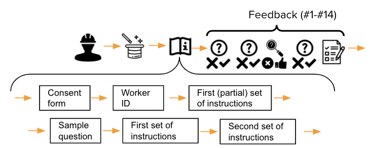
Figure 8. Structure of the initial part of the survey.

C.1. Consent

Purpose of research Study: The purpose of this study is to analyze how Amazon Mechanical Turk users interpret and use algorithmic predictions generated by decision support systems. We will perform statistical analysis to identify and extract patterns in the answers to this survey. Procedures: Your task is described in the following page. Risks/Discomforts: There are no risks for participating in this study beyond those associated with normal computer use and a minor risk of breach of confidentiality. Benefits: By completing this task, you will be more familiar with decision support systems used in the criminal justice setting. More broadly, this study may benefit society by improving the understanding of human-computer interaction. Voluntary participation and right to withdraw: Participation in this study is voluntary, and you can stop at any time. However, the survey needs to be completed for the HIT to be rewarded. Circumstances that could lead us to end your participation: We may decide to end your participation and/or not to reward the HIT for one of the following circumstances: (1) you fail at least one of the three attention checks (details in the instructions); (2) there is clear evidence that the questions have not been appropriately read and/or answered; (3) not all questions have been answered; (4) the survey has already been completed once, i.e. you are completing the survey for the second (or more) time. Confidentiality: Other than your Amazon Mechanical Turk serial number, we will collect the following demographic information: age, gender, race, level of education, and state of residence. We note that the Amazon Mechanical Turk serial number could be linked to your public profile page, so you might consider what information you choose to share on your public profile. These serial numbers will not be shared with anyone outside the research team and will only be used to handle financial transactions on the platform. Note, however, that de-identified data may be shared outside the research team. Compensation: If you satisfactorily complete the HIT/survey, you will receive a minimum compensation of 1.5$ for your participation. The extra reward (up to 5$) depends on your performance as described in the instructions. Payments are made via Amazon’s payment system. Contact information: [anonymized for submission] Clicking accept: By clicking the “Accept” button, you indicate that you are 18 years of age or older, that you voluntarily agree to participate in this study, and that you understand the information in this consent form. You have not waived any legal rights you otherwise would have as a participant in a research study.

C.2. Obtaining Worker ID

Please enter your Amazon Mechanical Turk Worker ID. We will use it only to process the payment. After entering the code, please press enter. Remember that if you have already completed this task in the past, you will not be rewarded.

If the ID already existed in our database (i.e., the worker had either completed the survey or failed an attention check in the past), the “Continue” button would not appear. If the ID was modified after having been verified by clicking the “Check if ID is new” button, then the “Continue” button was disabled.

C.3. First (partial) set of instructions

Task: In this task you will be shown demographic information and criminal history for individuals that have been arrested. These offenders have all been selected from real data. For every offender, we know whether they were rearrested within three years of release. Based on the available information, your task will be to predict whether the offenders were rearrested and to estimate the likelihood of this event. Questions: For each offender, you will be asked two questions: • $Q^{p}$: What is the likelihood of this offender being rearrested in the three years following release? For instance, 13% means that you think the probability of rearrest is 13%. You will use a slider to select your choice. The initial value of the slider is initialized at either 0 or 100. • $Q^{b}$: Do you think that the offender was rearrested in the three years following release? This question is similar to the first but asks only for a yes-no prediction. It is important to answer $Q^{p}$ before $Q^{b}$. Once you have answered $Q^{b}$, you may not be able to revise your answer in $Q^{p}$. In the three years following release, 42% of all offenders in the population were rearrested. The set of offenders that is shown to you is a representative sample of the entire population. You will evaluate 40 different offenders (+ 1 example and +3 attention checks). Throughout the survey, we will ask you a short series of questions to make you reflect on your answers. Now you will be shown an example. Please answer the questions in the example before proceeding to read further instructions.

C.4. First set of instructions

The first set of instructions included what had already been presented in §C.3, plus the following panel. Note that the third part of the survey (one question) was not mentioned in the instructions.

Structure of the survey: The survey consists of two consecutive parts: • First part (feedback, no algorithmic tool): You will start the survey with some example cases. For each case, after making your prediction, you will receive feedback on whether the offender was rearrested within three years of release. The feedback indicates whether your prediction (in response to $Q^{b}$) was accurate. If you predicted that the offender was not rearrested, but in fact they were, then your prediction was inaccurate. If you predicted that the offender was rearrested, but in fact they were not, then your prediction was inaccurate. This feedback can also help you refine your answers to $Q^{p}$. If you find that you are often assigning high probabilities of re-arrest to offenders that are not rearrested, then these probabilities may be too high. • Second part (no feedback, algorithmic tool): In this phase, you will make predictions but will not receive feedback about whether your predictions are accurate. For the questions in this part of the survey, you may also be shown the predictions of an algorithmic tool that was trained to predict re-arrest. You can incorporate the algorithmic tool’s predictions as an aid to help you evaluate, adjust, and revise your decisions. The tool is described below.
Algorithmic tool: The statistical model on which the tool is based was selected for being the most accurate among many statistical models. The tool has the following characteristics: • Target: The algorithmic tool has been trained to predict the likelihood of the offender’s re-arrest in the three years following release. For instance, if the algorithmic tool predicts that the likelihood of re-arrest is 60% for some offender, it means that this offender is going to be rearrested with probability 60%, according to this tool. • Information: The algorithmic tool has access to all the information that is available to you. In addition, the tool has also access to more detailed categories of past crimes and their frequency. • Calibration: Calibration is one of many benchmarks used to measure the quality of the predictions generated by algorithmic tools. Informally, an algorithmic tool is calibrated if on all the cases where it predicts, say, a 60% probability of re-arrest, in fact 60% of those offenders were rearrested. That does not mean that the algorithmic tool is actually good at making predictions. For example, an algorithmic tool that predicts that all offenders have a 42% probability of re-arrest would be perfectly calibrated! Indeed, these are group level estimates rather than precise estimates of individual likelihoods of re-arrest. The calibration properties of this tool are shown in the figure below.
Terminology: The following comparisons may be useful: • Misdemeanor vs felony: A misdemeanor is a crime considered to be of lower seriousness compared to a felony. Misdemeanors carry up to 1 year of jail in most states. Notice that misdemeanors are more serious than infractions. • Adult vs juvenile offenders under age 18 are considered juvenile.

C.5. Second set of instructions

Requirements: You must answer all questions for the survey to be valid and to complete the HIT. For each page, please answer all questions before proceeding to the following page. You will also need to answer the attention checks (described below) correctly. Attention checks: For three of the offenders, the answer to $Q^{b}$ will be explicitly mentioned in the description of the offender. You need to answer $Q^{b}$ accordingly. For those two offenders, you can select anything in $Q^{p}$. If you do not provide the correct answer to $Q^{b}$ (as specified in the text) for any of these two offenders, you will not be able to proceed with the rest of the survey. You will also not be able to retake the survey. If that’s the case, please return the HIT. Structure of rewards: The extra reward (up to 5$) is based on your performance in the testing phase. Performance is proportional to the accuracy of your answers in $Q^{p}$ and $Q^{b}$. For this evaluation, we will use your answers to $Q^{p}$ for 13 randomly chosen offenders (out of 25), and your answers to $Q^{b}$ for the remaining offenders. The measurements of performance on $Q^{p}$ and $Q^{b}$ use Brier score and accuracy respectively. The maximum reward for each question is 0.20$. For example, consider the case where you answer 30% ($Q^{p}$) and ”no” ($Q^{b}$), and the offender is not rearrested. In case $Q^{p}$ is selected, then you will receive 0.18$ = 0.20$*(1-(30%)²). In case $Q^{b}$ is selected, then you will receive the full 0.20$. Conversely, if the offender is rearrested, then you will receive 0.10$ in case of $Q^{p}$ and 0$ in case of $Q^{b}$. The payment schema has been designed to ensure that you will achieve the highest reward only by acting according to your true beliefs. In other words, you will get the highest reward answering both answers as well as you can.

C.6. Structure of the vignette

Show/hide informed consent form and instructions Offender [# OFFENDER] of 40 Demographics: The offender is [RACE] and [SEX]. She/he is [AGE] years old. Current charge: The offender has been charged with [CRIME CATEGORY]. Criminal history: The offender (if PRIOR ARRESTS>0){ has been arrested [PRIOR ARRESTS] time(s) and has been charged [PRIOR CHARGES] time(s). Of these arrests, (if PRIOR ARRESTS-JUVENILE>0){[PRIOR ARRESTS-JUVENILE] occurred when (s)he was a juvenile.} if(if PRIOR ARRESTS-JUVENILE=0){all occurred when she/he was an adult.} The previous charge was/charges were for the following categories of offenses: (if PRIOR CHARGES-TRAFFIC>0){traffic}, (if PRIOR CHARGES-DRUGS>0){drugs}, (if PRIOR CHARGES-SEXUAL ASSAULT>0){sexual assault}, (if PRIOR CHARGES-PUBLIC ORDER>0){public order}, (if PRIOR CHARGES-PUBLIC ADMINISTRATION>0){public administration}, (if PRIOR CHARGES-PROPERTY>0){property}, (if PRIOR CHARGES-WEAPONS>0){weapons}. Of these, [PRIOR CHARGES-VIOLENT] charge was/charges were for violent offenses.} (if PRIOR ARRESTS=0){has never been arrested before.} (if RAI shown){The algorithmic tool estimates that the offender’s likelihood of re-arrest is [$Q^{p}_{RAI}$].} (if RAI shown and non-anchoring setting){You have previously estimated that the offender’s likelihood of re-arrest is [$Q_{P}^{p}$]. You have previously estimated that the offender WAS (if $Q_{P}^{b}$=No){NOT} going to be rearrested.} What is the likelihood of this offender being rearrested in the three years following release? Do you think that the offender was rearrested in the three years following release? (if both answers given)       
(if feedback shown){(if $Y=Q_{P}^{b}$){ The offender WAS (if $Y$=No){NOT} rearrested in the three years following release.} (if $Y\neq Q_{P}^{b}$){ The offender WAS (if $Y$=No){NOT} rearrested in the three years following release.}}

Figure 9. Structure of the vignette. If the condition inside round brackets was met, then the value taken by the feature inside curly brackets was inserted into the text. For example, if PRIOR ARRESTS was “5”, then the generated sentence was “The offender has been arrested 5 times…”. $Q_{P}^{p}$ and $Q_{P}^{b}$ indicate the answers given by the participant without the assistance of the RAI to the first and second question in the vignette respectively. $Y$ indicates the outcome of the offender (i.e., rearrested or not). The RAIs presented in our work were trained only on the features, such as the offender’s prior number of arrests and age, and not on the full sentences.

C.7. Demographics

The participant is allowed to proceed only once all questions have been answered.

• How old are you? – [Integers from 18 to 80 to be selected using a slide bar] • What’s your gender? $\circ$ Female $\circ$ Male $\circ$ Transgender female $\circ$ Transgender male $\circ$ Not in these categories $\circ$ Prefer not to say • What’s your race/ethnicity? $\circ$ White $\circ$ Black or African American $\circ$ American Indian or Alaska Native $\circ$ Asian $\circ$ Native Hawaiian or Other Pacific Islander $\circ$ Not in these categories $\circ$ Prefer not to say • What’s your highest level of education? (already achieved) $\circ$ Less than high school degree $\circ$ Some college but no degree $\circ$ Associate degree $\circ$ Bachelor degree $\circ$ Graduate degree $\circ$ Not in these categories $\circ$ Prefer not to say • Where do you leave? – [Any of the US states to be selected using a drop-down list] • Have you ever used (even on Amazon MTurk) decision support systems (algorithmic tools) like the one described in the instructions? $\circ$ No $\circ$ Yes

C.8. Perception questions

The participant was allowed to proceed with the rest of the survey only once all questions other than the two free-response questions had been answered. Two of the questions in the second set of perception questions were affected by a technical issue in the initial batches of surveys. For the purpose of the data analysis, in question (1) we coded “Not confident at all” and “Slightly confident” as “Not confident”, “Somewhat confident” as “Neutral”, and the remaining two categories as “Confident”. In question (4), we coded the lowest two levels as “Below median accuracy”, the middle level as “Around median accuracy”, and the remaining two categories as “Above median accuracy”.

You have already evaluated [percentage of offenders already evaluated]% of the offenders! Please answer the following questions very carefully. (if second part of the survey){These questions concern all answers given in the testing phase of the survey. Do not take into account the decisions that you made during the first part of the survey.}
(if second part of the survey and non-anchoring setting){Consider only those predictions made after taking into account the algorithmic tool’s prediction.} (1) How confident were you, on average, in your yes-no predictions? $\circ$ Not confident at all $\circ$ Slightly confident $\circ$ Somewhat confident $\circ$ Moderately confident $\circ$ Extremely confident (2) If you happened to be very confident in some of your yes-no predictions, which characteristics of the offender made you so confident? Note that you may be not very confident on average, but still be extremely confident in some of your predictions.
(3) How many of your yes-no predictions do you think were correct? • [integers from 0 to 13, 14 or 25 to be selected using radio buttons] (4) How do you think that the accuracy of your yes-no predictions compares to the accuracies of other Amazon Mechanical Turk workers in this task?
The percentages in parentheses refer to the percentile rank of your accuracy in the distribution of all workersáccuracies. For example, say that there are other 100 workers. If you think that your accuracy is higher than the accuracies of 35 of them, then you should choose the percentile range (21-40%). Instead, if you think that your accuracy is higher than the accuracies of 85 of them, then you should choose the percentile range (81-100%). $\circ$ Among the lowest accuracies (0-20%) $\circ$ Lower than most accuracies (21-40%) $\circ$ Approximately equal to the median accuracy (41-60%) $\circ$ Higher than most accuracies (61-80%) $\circ$ Among the highest accuracies (81-100%) (5) (if second part of the survey){How often did you revise (change) your numerical prediction after seeing the prediction of the algorithmic tool?} • [integers from 0 to 13, 14, or 25 to be selected using radio buttons] (6) (if second part of the survey){How often did you revise (change) your yes-no prediction after seeing the prediction of the algorithmic tool?} • [integers from 0 to 13, 14, or 25 to be selected using radio buttons] (7) (if second part of the survey){If some of your yes-no predictions did not match the algorithmic toolś and you decided not to revise your yes-no predictions, why did you think that you were more accurate than the algorithmic tool?}

Appendix D Additional tables and figures

Category	Value	Census	Survey (n)
Sex (Census) /Gender (survey)	Male	49%	62.5% (332)
	Female	51%	36.5% (194)
Race	White	76%	76.1% (404)
	Black or AA	13%	14.7% (78)
	Asian	6%	6.2% (33)
	AI, AN, NH, PI	2%	1.7% (9)
Age	18-24 years old	7%	2.8% (15)
	25-34 years old	10%	44.1% (234)
	35-59 years old	25%	46% (244)
	60-78 years old	19%	6.8% (36)
Education	College degree or higher (age 25+)	32%	81.2% (419/516)
Region	Northeast	17%	16.9% (90)
	Midwest	21%	19.1% (102)
	West	24%	24.8% (132)
	South	38%	39.0% (207)
ML familiarity	Yes		44% (93)

Table 3. Comparison of the demographics of the sample in the survey with the estimates relative to the US population, obtained from the Census. The categories with only a few observations are excluded from the table. While we measure gender, the Census only provides estimates for sex.

Judges
Term	Estimate	Std.error	p.value
(Intercept)	-2.65	0.03	0.00
PRS	0.38	0.01	0.00
OGS	0.49	0.01	0.00

RAI
Term	Estimate	Std.error	p.value
(Intercept)	-1.07	0.03	0.00
PRS	0.42	0.01	0.00
OGS	0.08	0.01	0.00

Participants
Term	Estimate	Std.error	p.value
(Intercept)	-0.23	0.03	0.00
PRS	0.36	0.01	0.00
OGS	0.05	0.01	0.00

Table 4. Summaries of logistic regression models targeting the likelihood of incarceration (by judges) or the likelihood of predicted re-arrest (by RAI’s and participants’ predictions). The tables contain coefficients estimates, sandwich standard errors, and p-values relative to the null hypothesis that the coefficients are equal to zero. These models have been described in §4.4. The coefficients correspond to the offense gravity score (OGS) and to the prior record score (PRS). We note that the coefficient’s estimate of the offense gravity score is large in the model targeting the likelihood of incarceration, but small in the others.

Appendix E Comparison between the pilot study and the main experiment

Before running the experiment described in the main paper, we conducted a pilot study. The survey used in this study was in many ways similar to the survey in the main experiment, but also differed in the following aspects:

• participants were all shown the same set of offenders but in different orders. The offenders’ descriptions were based on a random sample drawn from the holdout set. The offenders were divided into two groups. The order was then randomized within groups.

• absence of bonus proportional to predictive performance and attention checks. In the pilot study, participants’ reward was not tied to their performance. We paid a fixed amount of $10 to all participants that completed the survey. We did not use attention checks.

• probability predictions were elicited using a slider instrument with a 10-point probability scale (0-10%, 11-20%, 21-30%, etc.).

In the pilot study, 24 of the 50 participants were assigned to the anchoring setting. Most of the findings from the pilot survey are virtually identical to those that were presented for the main study. In particular, the results of §4.1 (probability and binary predictions) and §4.2 (anchoring effects), which in principle could have been affected by the choice of the probability scale, held in this survey as well. We briefly discuss three results from the pilot study.

As in main study, we found that participants often predicted re-arrest even when they were assigning low values to its likelihood. Figure 12 shows the share of predicted re-arrests as a function of the participants’ risk estimates. The pattern in these predictions closely resembles what has been shown for the main experiment (see Figure 3). “Re-arrest” was predicted for approximately one fourth of the offenders for whom the risk estimate was between 41-50% or lower (mean re-arrest $Q^{b}$=26.4%) but “no re-arrest” was predicted for only 5% of the offenders whose risk estimates were equal or above 51%.

As in the main study, we found that the revised risk estimates of the participants in the non-anchoring setting were closer to the RAI’s than those of the participants assigned to the anchoring setting (mean $|Q^{p}_{P+RAI}-Q^{p}_{RAI}|$ in non-anchoring=$0.09$, in anchoring=$0.12$; $p_{TT}<\alpha$). The agreement between participants’ and RAI’s binary predictions, however, was slightly higher in the anchoring setting (mean $|Q^{b}_{P+RAI}-Q^{b}_{RAI}|$ in non-anchoring=32%, in anchoring=27%). Figure 13 shows the distribution of the probability predictions in the two settings for the 22 different offenders on which we tested anchoring effects. We observe that participants assigned to the non-anchoring setting often revised their risk estimates in the direction of the RAI’s. For most of the offenders the difference between the pre-registered predictions and the RAI’s estimates was fairly small. In cases where the pre-registered risk estimates were far from the RAI’s, the distribution of the revised predictions was similar to the one of the predictions made in the anchoring setting sometime (e.g., offender with id 22) but not in all cases (e.g., offenders with id 7 and 10).

Since the vignette did not change, the time spent by participants on the individual assessments can be compared across the two surveys. We separated the predictions made without the assistance of the RAI from those made in presence of the RAI. In case of the latter, we excluded those made in the non-anchoring setting. For both groups of predictions, we found that participants in the main study spent substantially more time than those in the pilot survey (both $p_{MW}<\alpha$). The right panel of Figure 12 shows the distribution of time spent on each assessment in the anchoring setting: The assessment took on average 16.1 seconds (median=11.4) for the participants in the main study but only 9.7 seconds (median=7) for those of the pilot study. It is possible that the introduction of attention checks, together with the incentive structure being tied to predictions accuracy, nudged participants into spending more time on the assessments or led to the exclusion of participants that were not paying adequate attention.

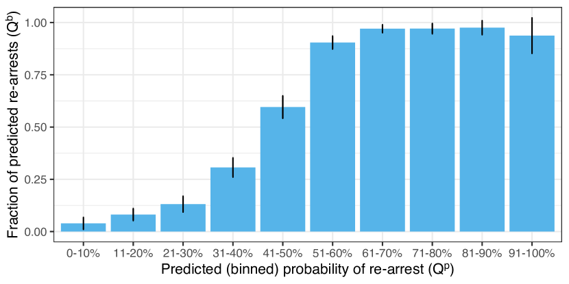
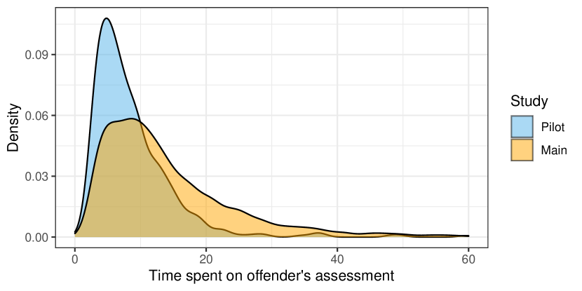
Figure 12. Analysis of the participants’ assessments in the pilot survey. (left) Share of predictions of re-arrest as a function of the probability predictions. Error bars indicate 95% confidence intervals. As in the main experiment (see Figure 3), we observe that binary predictions corresponding to re-arrest were frequent even for low values of the likelihood. (right) Comparison of time spent on each offender’s assessment in the anchoring setting in the pilot and main study. Here, we considered only the predictions made in presence of the RAI. These results indicate that assessments in the main study generally took longer than those in the pilot ($p_{MW}<\alpha$).

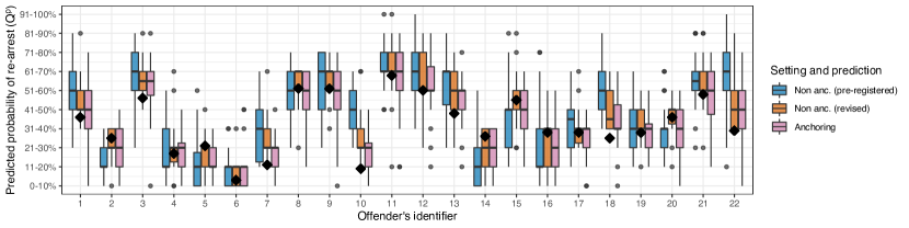
Figure 13. Analysis of participants’ and RAI’s predictions in the pilot study. Here, the anchoring effect was tested on a total of 22 different offenders. Each of the offenders corresponds to a separate identifier on the horizontal axis. The boxplots are relative to the pre-registered and revised risk estimates made in non-anchoring setting, and those made in the anchoring setting. Each boxplot corresponds to predictions made for a certain offender. The black squares indicate the prediction of the RAI that was shown to the participants.

References

- (1)
- Albright (2019) Alex Albright. 2019. If You Give a Judge a Risk Score: Evidence from Kentucky Bail Decisions. Technical Report. Working paper.
- Angelino et al. (2017) Elaine Angelino, Nicholas Larus-Stone, Daniel Alabi, Margo Seltzer, and Cynthia Rudin. 2017. Learning certifiably optimal rule lists for categorical data. The Journal of Machine Learning Research 18, 1 (2017), 8753–8830.
- Angwin et al. (2016) Julia Angwin, Jeff Larson, Surya Mattu, and Lauren Kirchner. 2016. Machine bias. ProPublica. See https://www. propublica. org/article/machine-bias-risk-assessments-in-criminal-sentencing (2016).
- Attali (2020) Dean Attali. 2020. shinyjs: Easily Improve the User Experience of Your Shiny Apps in Seconds. https://CRAN.R-project.org/package=shinyjs R package version 1.1.
- Austin and Ware (2020) James Austin and Wendy Ware. 2020. Why Bail Reform is Safe and Effective: The Case of Cook County. Available at SSRN 3599410 (2020).
- Bansal et al. (2021) Gagan Bansal, Tongshuang Wu, Joyce Zhou, Raymond Fok, Besmira Nushi, Ece Kamar, Marco Tulio Ribeiro, and Daniel Weld. 2021. Does the whole exceed its parts? the effect of ai explanations on complementary team performance. In Proceedings of the 2021 CHI Conference on Human Factors in Computing Systems. 1–16.
- Berk (2017) Richard Berk. 2017. An impact assessment of machine learning risk forecasts on parole board decisions and recidivism. Journal of Experimental Criminology 13, 2 (2017), 193–216.
- Berk et al. (2018) Richard Berk, Hoda Heidari, Shahin Jabbari, Michael Kearns, and Aaron Roth. 2018. Fairness in criminal justice risk assessments: The state of the art. Sociological Methods & Research (2018), 0049124118782533.
- Biswas et al. (2020) Arpita Biswas, Marta Kolczynska, Saana Rantanen, and Polina Rozenshtein. 2020. The Role of In-Group Bias and Balanced Data: A Comparison of Human and Machine Recidivism Risk Predictions. In Proceedings of the 3rd ACM SIGCAS Conference on Computing and Sustainable Societies. 97–104.
- Black et al. (1995) William C Black, Robert F Nease Jr, and Anna NA Tosteson. 1995. Perceptions of breast cancer risk and screening effectiveness in women younger than 50 years of age. JNCI: Journal of the National Cancer Institute 87, 10 (1995), 720–731.
- Breiman (2001) Leo Breiman. 2001. Random forests. Machine learning 45, 1 (2001), 5–32.
- Buçinca et al. (2021) Zana Buçinca, Maja Barbara Malaya, and Krzysztof Z Gajos. 2021. To trust or to think: cognitive forcing functions can reduce overreliance on AI in AI-assisted decision-making. Proceedings of the ACM on Human-Computer Interaction 5, CSCW1 (2021), 1–21.
- Bushway et al. (2012) Shawn D Bushway, Emily G Owens, and Anne Morrison Piehl. 2012. Sentencing guidelines and judicial discretion: Quasi-experimental evidence from human calculation errors. Journal of Empirical Legal Studies 9, 2 (2012), 291–319.
- Chang et al. (2020) Winston Chang, Joe Cheng, JJ Allaire, Yihui Xie, and Jonathan McPherson. 2020. shiny: Web Application Framework for R. https://CRAN.R-project.org/package=shiny R package version 1.4.0.2.
- Chen and Guestrin (2016) Tianqi Chen and Carlos Guestrin. 2016. Xgboost: A scalable tree boosting system. In Proceedings of the 22nd acm sigkdd international conference on knowledge discovery and data mining. 785–794.
- Chouldechova et al. (2018) Alexandra Chouldechova, Diana Benavides-Prado, Oleksandr Fialko, and Rhema Vaithianathan. 2018. A case study of algorithm-assisted decision making in child maltreatment hotline screening decisions. In Conference on Fairness, Accountability and Transparency. 134–148.
- Coston et al. (2021) Amanda Coston, Ashesh Rambachan, and Alexandra Chouldechova. 2021. Characterizing fairness over the set of good models under selective labels. arXiv preprint arXiv:2101.00352 (2021).
- Couper (2008) Mick P Couper. 2008. Designing effective web surveys. Cambridge University Press.
- Courts (2018) New Jersey Courts. 2018. Pretrial Release Recommendation Decision Making Framework (DMF). https://www.njcourts.gov/courts/assets/criminal/decmakframwork.pdf?cacheID=nDrtJn4
- De-Arteaga et al. (2020) Maria De-Arteaga, Riccardo Fogliato, and Alexandra Chouldechova. 2020. A Case for Humans-in-the-Loop: Decisions in the Presence of Erroneous Algorithmic Scores. In Proceedings of the 2020 CHI Conference on Human Factors in Computing Systems. 1–12.
- Delen (2010) Dursun Delen. 2010. A comparative analysis of machine learning techniques for student retention management. Decision Support Systems 49, 4 (2010), 498–506.
- DeMichele et al. (2018a) Matthew DeMichele, Peter Baumgartner, Michael Wenger, Kelle Barrick, Megan Comfort, and Shilpi Misra. 2018a. The public safety assessment: A re-validation and assessment of predictive utility and differential prediction by race and gender in kentucky. Available at SSRN 3168452 (2018).
- DeMichele et al. (2018b) Matthew DeMichele, Megan Comfort, Shilpi Misra, Kelle Barrick, and Peter Baumgartner. 2018b. The intuitive-override model: Nudging judges toward pretrial risk assessment instruments. Available at SSRN 3168500 (2018).
- Desmarais et al. (2020) Sarah L Desmarais, Samantha A Zottola, Sarah E Duhart Clarke, and Evan M Lowder. 2020. Predictive validity of pretrial risk assessments: A systematic review of the literature. Criminal Justice and Behavior (2020), 0093854820932959.
- Dieterich et al. (2016) William Dieterich, Christina Mendoza, and Tim Brennan. 2016. COMPAS Risk Scales: Demonstrating Accuracy Equity and Predictive Parity. (2016).
- Dressel and Farid (2018) Julia Dressel and Hany Farid. 2018. The accuracy, fairness, and limits of predicting recidivism. Science advances 4, 1 (2018), eaao5580.
- Efron (1971) Bradley Efron. 1971. Forcing a sequential experiment to be balanced. Biometrika 58, 3 (1971), 403–417.
- Englich et al. (2005) Birte Englich, Thomas Mussweiler, and Fritz Strack. 2005. The last word in court—A hidden disadvantage for the defense. Law and Human Behavior 29, 6 (2005), 705–722.
- Englich et al. (2006) Birte Englich, Thomas Mussweiler, and Fritz Strack. 2006. Playing dice with criminal sentences: The influence of irrelevant anchors on experts’ judicial decision making. Personality and Social Psychology Bulletin 32, 2 (2006), 188–200.
- Enough and Mussweiler (2001) Birte Enough and Thomas Mussweiler. 2001. Sentencing under uncertainty: Anchoring effects in the courtroom 1. Journal of applied social psychology 31, 7 (2001), 1535–1551.
- Epley and Gilovich (2005) Nicholas Epley and Thomas Gilovich. 2005. When effortful thinking influences judgmental anchoring: differential effects of forewarning and incentives on self-generated and externally provided anchors. Journal of Behavioral Decision Making 18, 3 (2005), 199–212.
- Evans et al. (2004) Jonathan St BT Evans, David E Over, et al. 2004. If: Supposition, pragmatics, and dual processes. Oxford University Press, USA.
- Fogliato et al. (2020) Riccardo Fogliato, Alexandra Chouldechova, and Max G’Sell. 2020. Fairness Evaluation in Presence of Biased Noisy Labels. In International Conference on Artificial Intelligence and Statistics. PMLR, 2325–2336.
- Fort et al. (2011) Karën Fort, Gilles Adda, and K Bretonnel Cohen. 2011. Amazon mechanical turk: Gold mine or coal mine? Computational Linguistics 37, 2 (2011), 413–420.
- Gino and Moore (2007) Francesca Gino and Don A Moore. 2007. Effects of task difficulty on use of advice. Journal of Behavioral Decision Making 20, 1 (2007), 21–35.
- Gluck and Bower (1988) Mark A Gluck and Gordon H Bower. 1988. From conditioning to category learning: An adaptive network model. Journal of Experimental Psychology: General 117, 3 (1988), 227.
- Grant (2019) Glenn Grant. 2019. Report to the Governor and the Legislature. New Jersey Courts. (2019).
- Green and Chen (2019a) Ben Green and Yiling Chen. 2019a. Disparate interactions: An algorithm-in-the-loop analysis of fairness in risk assessments. In Proceedings of the Conference on Fairness, Accountability, and Transparency. ACM, 90–99.
- Green and Chen (2019b) Ben Green and Yiling Chen. 2019b. The principles and limits of algorithm-in-the-loop decision making. Proceedings of the ACM on Human-Computer Interaction 3, CSCW (2019), 1–24.
- Grgić-Hlača et al. (2019) Nina Grgić-Hlača, Christoph Engel, and Krishna P Gummadi. 2019. Human decision making with machine assistance: An experiment on bailing and jailing. Proceedings of the ACM on Human-Computer Interaction 3, CSCW (2019), 1–25.
- Guthrie et al. (2000) Chris Guthrie, Jeffrey J Rachlinski, and Andrew J Wistrich. 2000. Inside the judicial mind. Cornell L. Rev. 86 (2000), 777.
- Hyatt and Chanenson (2016) Jordan Hyatt and Steven L Chanenson. 2016. The use of risk assessment at sentencing: Implications for research and policy. Villanova Law/Public Policy Research Paper 2017-1040 (2016).
- Jung et al. (2020) Jongbin Jung, Sharad Goel, Jennifer Skeem, et al. 2020. The limits of human predictions of recidivism. Science advances 6, 7 (2020), eaaz0652.
- Kahneman and Tversky (2013) Daniel Kahneman and Amos Tversky. 2013. Prospect theory: An analysis of decision under risk. In Handbook of the fundamentals of financial decision making: Part I. World Scientific, 99–127.
- Kale et al. (2020) Alex Kale, Matthew Kay, and Jessica Hullman. 2020. Visual reasoning strategies for effect size judgments and decisions. IEEE Transactions on Visualization and Computer Graphics (2020).
- Kallus and Zhou (2019) Nathan Kallus and Angela Zhou. 2019. Assessing Disparate Impact of Personalized Interventions: Identifiability and Bounds. In Advances in Neural Information Processing Systems. 3426–3437.
- Kleinberg et al. (2017) Jon Kleinberg, Himabindu Lakkaraju, Jure Leskovec, Jens Ludwig, and Sendhil Mullainathan. 2017. Human decisions and machine predictions. The quarterly journal of economics 133, 1 (2017), 237–293.
- Koehler (1996) Jonathan J Koehler. 1996. The base rate fallacy reconsidered: Descriptive, normative, and methodological challenges. Behavioral and brain sciences 19, 1 (1996), 1–17.
- Kuhn and Wickham (2020) Max Kuhn and Hadley Wickham. 2020. tidymodels: Easily Install and Load the ’Tidymodels’ Packages. https://CRAN.R-project.org/package=tidymodels R package version 0.1.0.
- Lai and Tan (2019) Vivian Lai and Chenhao Tan. 2019. On human predictions with explanations and predictions of machine learning models: A case study on deception detection. In Proceedings of the Conference on Fairness, Accountability, and Transparency. 29–38.
- Lakkaraju et al. (2017) Himabindu Lakkaraju, Jon Kleinberg, Jure Leskovec, Jens Ludwig, and Sendhil Mullainathan. 2017. The selective labels problem: Evaluating algorithmic predictions in the presence of unobservables. In Proceedings of the 23rd ACM SIGKDD International Conference on Knowledge Discovery and Data Mining. 275–284.
- Lipkus et al. (2001) Isaac M Lipkus, Greg Samsa, and Barbara K Rimer. 2001. General performance on a numeracy scale among highly educated samples. Medical decision making 21, 1 (2001), 37–44.
- Mallari et al. (2020) Keri Mallari, Kori Inkpen, Paul Johns, Sarah Tan, Divya Ramesh, and Ece Kamar. 2020. Do I Look Like a Criminal? Examining how Race Presentation Impacts Human Judgement of Recidivism. In Proceedings of the 2020 CHI Conference on Human Factors in Computing Systems. 1–13.
- Manski (2004) Charles F Manski. 2004. Measuring expectations. Econometrica 72, 5 (2004), 1329–1376.
- Mason and Suri (2012) Winter Mason and Siddharth Suri. 2012. Conducting behavioral research on Amazon’s Mechanical Turk. Behavior research methods 44, 1 (2012), 1–23.
- Metz and Satariano (2020) Cate Metz and Adam Satariano. 2020. An Algorithm that Grants Freedom, or Takes it Away. https://www.nytimes.com/2020/02/06/technology/predictive-algorithms-crime.html
- Mussweiler and Strack (2000) Thomas Mussweiler and Fritz Strack. 2000. Numeric judgments under uncertainty: The role of knowledge in anchoring. Journal of experimental social psychology 36, 5 (2000), 495–518.
- Nagin et al. (2013) Daniel S Nagin et al. 2013. Deterrence: A review of the evidence by a criminologist for economists. Annual Review of Economics 5, 1 (2013), 83–105.
- Nisbett and Wilson (1977) Richard E Nisbett and Timothy D Wilson. 1977. Telling more than we can know: verbal reports on mental processes. Psychological review 84, 3 (1977), 231.
- O’Hagan et al. (2006) Anthony O’Hagan, Caitlin E Buck, Alireza Daneshkhah, J Richard Eiser, Paul H Garthwaite, David J Jenkinson, Jeremy E Oakley, and Tim Rakow. 2006. Uncertain judgements: eliciting experts’ probabilities. John Wiley & Sons.
- on Sentencing (2020a) Pennsylvania Commission on Sentencing. 2020a. An Overview of the Sentence Risk Assessment Instrument. https://sentencing.umn.edu/sites/sentencing.umn.edu/files/pennsylvania_overview_of_the_sentencing_risk_assessment_instrument_2017.pdf
- on Sentencing (2020b) The Pennsylvania Commission on Sentencing. 2020b. Judicial System General Provisions. Part VIII Criminal Sentencing. Chapter 305. Sentence Risk Assessment Instrument. http://pcs.la.psu.edu/guidelines/sentence-risk-assessment-instrument/sentence-risk-assessment-instrument-guideline-text
- Paravisini and Schoar (2013) Daniel Paravisini and Antoinette Schoar. 2013. The incentive effect of scores: Randomized evidence from credit committees. Technical Report. National Bureau of Economic Research.
- Pennsylvania Commission on Sentencing (2020) Pennsylvania Commission on Sentencing. 2020. Sentencing Guidelines and Implementation Manuals. http://pcs.la.psu.edu/guidelines/sentencing/sentencing-guidelines-and-implementation-manuals
- Poursabzi-Sangdeh et al. (2021) Forough Poursabzi-Sangdeh, Daniel G Goldstein, Jake M Hofman, Jennifer Wortman Wortman Vaughan, and Hanna Wallach. 2021. Manipulating and measuring model interpretability. In Proceedings of the 2021 CHI Conference on Human Factors in Computing Systems. 1–52.
- Prelec (1998) Drazen Prelec. 1998. The probability weighting function. Econometrica (1998), 497–527.
- R Core Team (2019) R Core Team. 2019. R: A Language and Environment for Statistical Computing. R Foundation for Statistical Computing, Vienna, Austria. https://www.R-project.org/
- Raghavan et al. (2020) Manish Raghavan, Solon Barocas, Jon Kleinberg, and Karen Levy. 2020. Mitigating bias in algorithmic hiring: Evaluating claims and practices. In Proceedings of the 2020 Conference on Fairness, Accountability, and Transparency. 469–481.
- Redmiles et al. (2019) Elissa M Redmiles, Sean Kross, and Michelle L Mazurek. 2019. How well do my results generalize? comparing security and privacy survey results from mturk, web, and telephone samples. In 2019 IEEE Symposium on Security and Privacy (SP). IEEE, 1326–1343.
- Roster et al. (2015) Catherine A Roster, Lorenzo Lucianetti, and Gerald Albaum. 2015. Exploring slider vs. categorical response formats in web-based surveys. Journal of Research Practice 11, 1 (2015), D1–D1.
- Saxena et al. (2020) Devansh Saxena, Karla Badillo-Urquiola, Pamela J Wisniewski, and Shion Guha. 2020. A Human-Centered Review of Algorithms used within the US Child Welfare System. In Proceedings of the 2020 CHI Conference on Human Factors in Computing Systems. 1–15.
- Schwartz et al. (1997) Lisa M Schwartz, Steven Woloshin, William C Black, and H Gilbert Welch. 1997. The role of numeracy in understanding the benefit of screening mammography. Annals of internal medicine 127, 11 (1997), 966–972.
- Scurich and John (2011) Nicholas Scurich and Richard S John. 2011. The effect of framing actuarial risk probabilities on involuntary civil commitment decisions. Law and human behavior 35, 2 (2011), 83–91.
- Sendak et al. (2020) Mark Sendak, Madeleine Clare Elish, Michael Gao, Joseph Futoma, William Ratliff, Marshall Nichols, Armando Bedoya, Suresh Balu, and Cara O’Brien. 2020. ” The human body is a black box” supporting clinical decision-making with deep learning. In Proceedings of the 2020 Conference on Fairness, Accountability, and Transparency. 99–109.
- Skeem and Lowenkamp (2020) Jennifer Skeem and Christopher Lowenkamp. 2020. Using algorithms to address trade-offs inherent in predicting recidivism. Behavioral Sciences & the Law (2020).
- Skeem and Lowenkamp (2016) Jennifer L Skeem and Christopher T Lowenkamp. 2016. Risk, race, and recidivism: Predictive bias and disparate impact. Criminology 54, 4 (2016), 680–712.
- Stevenson (2018) Megan Stevenson. 2018. Assessing risk assessment in action. Minn. L. Rev. 103 (2018), 303.
- Tan et al. (2018) Sarah Tan, Julius Adebayo, Kori Inkpen, and Ece Kamar. 2018. Investigating Human+ Machine Complementarity for Recidivism Predictions. arXiv preprint arXiv:1808.09123 (2018).
- Tibshirani (1996) Robert Tibshirani. 1996. Regression shrinkage and selection via the lasso. Journal of the Royal Statistical Society: Series B (Methodological) 58, 1 (1996), 267–288.
- Tversky and Kahneman (1974) Amos Tversky and Daniel Kahneman. 1974. Judgment under uncertainty: Heuristics and biases. science 185, 4157 (1974), 1124–1131.
- Vaccaro and Waldo (2019) Michelle Vaccaro and Jim Waldo. 2019. The Effects of Mixing Machine Learning and Human Judgment. Queue 17, 4 (2019), 30.
- Visschers et al. (2009) Vivianne HM Visschers, Ree M Meertens, Wim WF Passchier, and Nanne NK De Vries. 2009. Probability information in risk communication: a review of the research literature. Risk Analysis: An International Journal 29, 2 (2009), 267–287.
- Wickham et al. (2019) Hadley Wickham, Mara Averick, Jennifer Bryan, Winston Chang, Lucy D’Agostino McGowan, Romain François, Garrett Grolemund, Alex Hayes, Lionel Henry, Jim Hester, Max Kuhn, Thomas Lin Pedersen, Evan Miller, Stephan Milton Bache, Kirill Müller, Jeroen Ooms, David Robinson, Dana Paige Seidel, Vitalie Spinu, Kohske Takahashi, Davis Vaughan, Claus Wilke, Kara Woo, and Hiroaki Yutani. 2019. Welcome to the tidyverse. Journal of Open Source Software 4, 43 (2019), 1686. https://doi.org/10.21105/joss.01686
- Wilson (2004) Timothy D Wilson. 2004. Strangers to ourselves. Harvard University Press.
- Yin et al. (2019) Ming Yin, Jennifer Wortman Vaughan, and Hanna Wallach. 2019. Understanding the Effect of Accuracy on Trust in Machine Learning Models. In Proceedings of the 2019 CHI Conference on Human Factors in Computing Systems. ACM, 279.
- Zhang et al. (2020) Yunfeng Zhang, Q Vera Liao, and Rachel KE Bellamy. 2020. Effect of confidence and explanation on accuracy and trust calibration in AI-assisted decision making. In Proceedings of the 2020 Conference on Fairness, Accountability, and Transparency. 295–305.