A multi-frequency sampling method for the inverse source problems with sparse measurements

Abstract

We consider the inverse source problems with multi-frequency sparse near field measurements. In contrast to the existing near field operator based on the integral over the space variable, a multi-frequency near field operator is introduced based on the integral over the frequency variable. A factorization of this multi-frequency near field operator is further given and analysed. Motivated by such a factorization, we introduce a multi-frequency sampling method to reconstruct the source support. Its theoretical foundation is then derived from the properties of the factorized operators and a properly chosen point spread function. Numerical examples are provided to illustrate the multi-frequency sampling method with sparse near field measurements. Finally we briefly discuss how to extend the near field case to the far field case.

Keywords: sampling method; multi-frequency; sparse data; inverse source problems

AMS subject classifications: 35P25, 45Q05, 78A46, 74B05

1 Introduction

Inverse scattering merits numerous applications in radar, medical imaging, geophysics, non-destructive testing, and many others. In the last thirty years, sampling methods for shape reconstruction in inverse scattering problems have attracted a lot of interest. Classical examples include the linear sampling method [14] and the factorization method [27]. Such methods are independent of any a priori information on the geometry and physical properties of the unknown scatterers. The theoretical foundation of these sampling methods is the factorization of the far field or the near field operator $F$ in the form

$$F=\tilde{H}TH$$ (1.1)

with some coercive operator $T$ and a pair of operators $H$ and $\tilde{H}$ (in some cases $\tilde{H}$ is the adjoint of $H$). The operators $H$, $\tilde{H}$, and $T$ may vary in different inverse scattering problems. With this factorization, one may derive a necessary and sufficient criteria to reconstruct the scatterer and design an indicator function which is large inside the underlying scatterer and relatively small outside. We refer to the monographs [12, 15, 28] for a comprehensive introduction.

There have been recent efforts on other types of sampling methods such as orthogonality sampling method [19, 21, 33], direct sampling method [4, 5, 22, 25, 30], single-shot method [29], reverse time migration [13], and other direct reconstruction methods [2, 3]. These sampling methods inherit many advantages of the classical ones. The main feature of these sampling methods is that only inner product of the measurements with some suitably chosen functions is involved in the imaging function and thus these sampling methods are robust to noises. Recently, a sampling type method is of the form [31, 32]

$$I(z)=\left|(Fg_{z},\tilde{g}_{z})\right|$$ (1.2)

with suitably chosen $g_{z}$ and $\tilde{g}_{z}$ such that

• $\tilde{H}^{*}\tilde{g}_{z}=Hg_{z}$ where $\tilde{H}^{*}$ is the adjoint of $\tilde{H}$ given in (1.1);

• $|Hg_{z}|$ is a point spread function that peaks when the sampling point $z$ located on the boundaries of the unknown scatterers (or inside the scatterers in different problems).

Based on the factorization of the far field or near field operator (1.1), we deduce that their exists two positive constant $c$ and $C$ such that

$$c\|Hg_{z}\|^{2}\leq I(z)\leq C\|Hg_{z}\|^{2}.$$ (1.3)

This theoretical foundation (1.3) implies that $I(z)$ is qualitatively the same as a suitable norm of the point spread function $|Hg_{z}|$, i.e.

$$I(z)\approx\|Hg_{z}\|^{2},$$

which allows us to design a robust and fast imaging algorithm.

In this work, we apply the above framework to introduce a multi-frequency sampling method for the inverse source problems using sparse measurements. Most of the works in literature assume that the measurements are taken all around the unknown source. In this full-aperture case, uniqueness of the source function $f$ can be proved using the Fourier transform, see for instance [7, 18]. We refer to [9] for an iterative method with respect to frequencies. Recently, some non-iterative methods have been proposed. In particular, [36, 37] studied a Fourier method to reconstruct the source function and [11, 38] investigated the direct sampling methods for identifying the point sources. One practical situation involves sparse measurements, i.e. measurements that are only available at a limited number of sensors. Generally, neither the source nor its support is uniquely determined by the sparse data. Some lower bounds for the support of a source have been established in [35] in terms of multi-frequency sparse far field measurements. If it is known a priori that the source is a combination of point sources, uniqueness for the locations and the scattering strengths can be established [23, 24, 26]. We refer to [20] and [1] for a factorization method and a direct sampling method, respectively, using multi-frequency sparse far field measurements. For the multi-frequency sparse near field measurements, the corresponding uniqueness and direct sampling method can be found in a recent work [26]. Following the framework (1.1)–(1.3) developed in [31, 32] for inverse obstacle/medium scattering problems, this work contributes to a multi-frequency sampling method for the inverse source problems with sparse measurements.

The paper is further organized as follows. We introduce the model of the forward problem and inverse source problem with multi-frequency sparse near field measurements in Section 2. In contrast to the existing near field operator based on the integral over the space variable, we define a multi-frequency near field operator for each measurement point based on the integral over the frequency variable. We further provide a factorization of this multi-frequency near field operator in the form (1.1) in Section 3. This factorization is one of the key ingredients in our multi-frequency sampling method. In Section 4, we design an imaging function with properly chosen $g_{z}$ and $\tilde{g}_{z}$. Furthermore we provide its theoretical foundation based on the factorization and a point spread function. Section 5 presents numerical examples to illustrate our multi-frequency sampling method with sparse near field measurements. Finally in Section 6 we briefly discuss how to extend the near field case to the far field case.

2 Mathematical model and the inverse problem

We consider the acoustic wave propagation due to a source $f$ in a homogeneous isotropic medium in ${\mathbb{R}}^{3}$ with speed of sound $c>0$. Denote by $D$ the support of the unknown source, which is a bounded Lipschitz domain in ${\mathbb{R}}^{3}$ with connected complement ${\mathbb{R}}^{3}\backslash\overline{D}$. The mathematical model of the scattering of time-harmonic wave leads to the nonhomogeneous Helmholtz equation

$$\Delta u^{s}+k^{2}u^{s}=f\quad\mbox{in}\,\,{\mathbb{R}}^{3},$$ (2.4)

where the wave number is $k=\omega/c$ with frequency $\omega>0$. The scattered field $u^{s}$ is required to satisfy the Sommerfeld radiation condition

$$\lim_{r=|x|\rightarrow\infty}r\Big{(}\frac{\partial u^{s}}{\partial r}-iku^{s}\Big{)}=0$$ (2.5)

uniformly for all directions $x/|x|$. Throughout the paper we write $u^{s}(\cdot,k)$ to emphasize the dependence on the wave number $k$. If not otherwise stated, we consider multiple wave numbers in a bounded interval, i.e.,

$$k\in K:=(0,k_{max}],$$ (2.6)

with an upper bound $k_{max}>0$.

The unique radiating solution $u^{s}$ to the scattering problem (2.4)-(2.5) takes the form

$$u^{s}(x,k)=\int_{D}\Phi_{k}(x,y)f(y)ds(y),\quad x\in{\mathbb{R}}^{3},\,k\in K$$ (2.7)

with

$$\Phi_{k}(x,y):=\frac{e^{ik|x-y|}}{4\pi|x-y|},\quad x\not=y$$

being the fundamental solution to the Helmholtz equation.

A practical inverse problem is to recover the source support $D$ from the multi-frequency sparse measurements where the scattered fields are available at finitely many points in the set

$$\Gamma_{L}:=\{x_{1},x_{2},\cdots,x_{L}\}\subset{\mathbb{R}}^{3}\backslash\overline{D}.$$

Accordingly, we obtain the following multi-frequency sparse near field measurements

$$\mathbb{M}_{N}:=\{u^{s}(x,k)\,|\,x\in\Gamma_{L},\,\,k\in K\}.$$ (2.8)

Generally speaking, uniqueness of the source support $D$ does not hold from the near field measurements $\mathbb{M}_{N}$. An approximate support containing $D$ can be uniquely determined. We refer to [1, 20, 26, 35] for more details on the uniqueness.

3 The multi-frequency near field operator and its factorization

In this section, we introduce a multi-frequency near field operator given by the measurements $\mathbb{M}_{N}$ (2.8) and study its factorization which plays a key role in the analysis and design of our imaging algorithm. We assume that the source function $f\in L^{2}({\mathbb{R}}^{3})$ is real-valued and satisfies that

$$C_{f}\geq f(x)\geq c_{f}\quad\mbox{or}\quad-C_{f}\leq f(x)\leq-c,\quad x\in\,D$$ (3.9)

for two constants $C_{f}>c_{f}>0$.

To begin with, we define the scattered fields with negative frequencies by

$$u^{s}(x,-k):=\overline{u^{s}(x,k)},\quad x\in\Gamma_{L},\,k\in K.$$

Note that $f$ is real-valued, we then have the following integral representation for the scattered fields

$$u^{s}(x,k)=\int_{D}\Phi_{k}(x,y)f(y)ds(y),\quad x\in\Gamma_{L},\,k\in[-k_{max},k_{max}]\backslash\{0\}.$$ (3.10)

For each $x\in\Gamma_{L}$, we define the integral operator $\mathcal{N}_{x}:L^{2}(K)\rightarrow L^{2}(K)$ by

$$(\mathcal{N}_{x}g)(t):=\int_{K}u^{s}(x,t-s)g(s)ds,\quad t\in K,$$ (3.11)

which we will call the multi-frequency near field operator. Different from the usual near field operator which uses full-aperture measurements with a single frequency, this operator seeks to explore the relations among different frequencies. The factorization of the usual near field operator plays an important role in the modified sampling method [32] so that no asymptotic assumptions on the distance between the measurement surface and the scatterers were made there. In the same spirit, we seek to given a characterization of the unknown source support $D$ by the multi-frequency near field operator $\mathcal{N}_{x}$ together with its factorization.

To factorize $\mathcal{N}_{x}$, we first define $\mathcal{P}_{x}:L^{2}(D)\rightarrow L^{2}(K)$ by

$$(\mathcal{P}_{x}\psi)(t):=\int_{D}e^{it|x-y|}\psi(y)dy,\quad t\in K.$$ (3.12)

We can directly derive that its adjoint $\mathcal{P}^{\ast}_{x}:L^{2}(K)\rightarrow L^{2}(D)$ is given by

$$(\mathcal{P}^{\ast}_{x}\phi)(y):=\int_{K}e^{-is|x-y|}\phi(s)ds,\quad y\in D.$$ (3.13)

Finally we define the operator $\mathcal{T}_{x}:L^{2}(D)\rightarrow L^{2}(D)$ by

$$(\mathcal{T}_{x}h)(y):=\frac{f(y)}{4\pi|x-y|}h(y),\quad y\in D.$$ (3.14)

It directly follows that $\mathcal{T}_{x}$ is a self-adjoint operator since $f$ is real-valued. Now we are ready to give the following factorization of the multi-frequency near field operator $\mathcal{N}_{x}$.

Theorem 3.1.

For each $x\in\Gamma_{L}$, the following factorization holds

$$\mathcal{N}_{x}=\mathcal{P}_{x}\mathcal{T}_{x}\mathcal{P}^{\ast}_{x}.$$ (3.15)

Proof.

Inserting the integral representation (3.10) into the definition (3.11) of the multi-frequency near field operator $\mathcal{N}_{x}$, we have that

$$(\mathcal{N}_{x}g)(t) = \int_{K}\int_{D}\frac{e^{i(t-s)|x-y|}}{4\pi|x-y|}f(y)dyg(s)ds$$

$$= \int_{D}e^{it|x-y|}\frac{f(y)}{4\pi|x-y|}\int_{K}e^{-is|x-y|}g(s)dsdy$$

$$= (\mathcal{P}_{x}\mathcal{T}_{x}\mathcal{P}^{\ast}_{x}g)(t),\quad t\in K.$$

This completes the proof. ∎

Theorem 3.1 provides a symmetric factorization which allows us to study a factorization method, which is expected to be similar to the factorization method using multi-frequency far field measurements [20]. Alternatively, our goal here is to utilize this factorization to introduce a multi-frequency sampling method. We remark that this type of sampling method may still work even in the case of non-symmetric factorization (see for instance [32]).

4 The multi-frequency sampling method

This section is devoted to a multi-frequency sampling method using sparse near field measurements $\mathbb{M}_{N}$ (2.7). To begin with, we provide the following property of the middle operator $\mathcal{T}_{x}$.

Lemma 4.1.

Assume that $f\in L^{2}({\mathbb{R}}^{3})$ satisfies (3.9). For each $x\in\Gamma_{L}$, the operator $\mathcal{T}_{x}:L^{2}(D)\rightarrow L^{2}(D)$ is self-adjoint and coercive, i.e.

$$\frac{c_{f}}{4\pi r_{2}}\|h\|^{2}_{L^{2}(D)}\leq|(\mathcal{T}_{x}h,h)_{L^{2}(D)}|\leq\frac{C_{f}}{4\pi r_{1}}\|h\|^{2}_{L^{2}(D)},\quad\forall h\in L^{2}(D),$$ (4.16)

where

$$r_{1}:=\inf\{|x-y|\,:\,y\in D\}\quad\mbox{and}\quad r_{2}:=\sup\{|x-y|\,:\,y\in D\}.$$ (4.17)

Proof.

Recall the definition of $\mathcal{T}_{x}$ (3.14), we have that

$$(\mathcal{T}_{x}h,h)_{L^{2}(D)}=\int_{D}\frac{f(y)}{4\pi|x-y|}|h(y)|^{2}dy.$$

Note from the assumption (3.9) that

$$C_{f}\geq f(x)\geq c_{f}\quad\mbox{or}\quad-C_{f}\leq f(x)\leq-c,\quad x\in\,D,$$ (4.18)

then the inequality (4.16) follows by the definition of $r_{1}$ and $r_{2}$. This proves the lemma. ∎

We now prove the following theorem which plays an important role in the analysis and design of our imaging algorithm.

Theorem 4.2.

Assume that $f\in L^{2}({\mathbb{R}}^{3})$ satisfies (3.9). For each $x\in\Gamma_{L}$, the following inequality holds

$$\frac{c_{f}}{4\pi r_{2}}\|\mathcal{P}^{\ast}_{x}g\|^{2}_{L^{2}(D)}\leq|(\mathcal{N}_{x}g,g)_{L^{2}(K)}|\leq\frac{C_{f}}{4\pi r_{1}}\|\mathcal{P}^{\ast}_{x}g\|^{2}_{L^{2}(D)},\quad\forall g\in L^{2}(K).$$

Proof.

With the help of the factorization (3.15) in Theorem 3.1, we have that

$$(\mathcal{N}_{x}g,g)_{L^{2}(K)}=(\mathcal{P}_{x}T_{x}\mathcal{P}^{\ast}_{x}g,g)_{L^{2}(K)}=(T_{x}\mathcal{P}^{\ast}_{x}g,\mathcal{P}^{\ast}_{x}g)_{L^{2}(D)}.$$

Then the theorem follows from Lemma 4.1. This proves the theorem. ∎

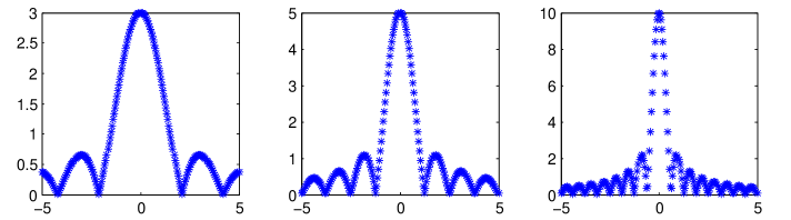
Figure 1: Plot of $|(\mathcal{P}^{\ast}_{x}g_{xz})(y)|$ as a function of $\mathbbm{t}$ in $[-5,5]$. Left: $k_{max}=3$;  Middle: $k_{max}=5$;  Right: $k_{max}=10$.

The above theorem implies that $|(\mathcal{N}_{x}g,g)_{L^{2}(K)}|$ is qualitatively the same as $\|\mathcal{P}^{\ast}_{x}g\|^{2}_{L^{2}(D)}$. The following theorem gives a properly chosen $g_{xz}$ such that $(\mathcal{P}^{\ast}_{x}g_{xz})$ is a point spread function.

Theorem 4.3.

For each $x\in\Gamma_{L}$ and $z\in{\mathbb{R}}^{3}$, we define $g_{xz}\in L^{2}(K)$ by

$$g_{xz}(s):=e^{is|x-z|},\quad s\in K.$$ (4.19)

It holds that

$$(\mathcal{P}^{\ast}_{x}g_{xz})(y)=\Bigg{\{}\begin{array}[]{cc}k_{max}&\mbox{if }\mathbbm{t}=0\\ \frac{e^{i\mathbbm{t}k_{max}}-1}{\mathbbm{t}}&\mbox{if }\mathbbm{t}\not=0\end{array},\quad y\in D,$$ (4.22)

where $\mathbbm{t}:=|x-z|-|x-y|$. In particular, $(\mathcal{P}^{\ast}_{x}g_{xz})(y)=(\mathcal{P}^{\ast}_{x}g_{xz})(y^{*})$ if $|y-x|=|y^{*}-x|$.

Furthermore,

$$|(\mathcal{P}^{\ast}_{x}g_{xz})(y)|\leq k_{max},\quad y\in D,$$

where “$=$” holds if and only if $\mathbbm{t}=0$. The following asymptotic holds

$$|(\mathcal{P}^{\ast}_{x}g_{xz})(y)|=\mathcal{O}\left(\frac{1}{\mathbbm{t}}\right),\quad\mathbbm{t}\rightarrow\infty.$$

Proof.

From the definition of $\mathcal{P}^{\ast}_{x}$ (3.13), we have that

$$(\mathcal{P}^{\ast}_{x}g_{xz})(y)=\int_{0}^{k_{max}}e^{is(|x-z|-|x-y|)}ds,\quad y\in D.$$

Then equation (4.22) follows from a direct computation. It then follows that $(\mathcal{P}^{\ast}_{x}g_{xz})(y)=(\mathcal{P}^{\ast}_{x}g_{xz})(y^{*})$ if $|y-x|=|y^{*}-x|$.

Furthermore we derive that

$$\left|(\mathcal{P}^{\ast}_{x}g_{xz})(y)\right|=\left|\int_{0}^{k_{max}}e^{is\mathbbm{t}}ds\right|\leq\int_{0}^{k_{max}}\left|e^{is\mathbbm{t}}\right|ds\leq k_{max},\quad y\in D,$$

where “$=$” holds if and only if $\mathbbm{t}=0$.

Finally the asymptotic of $|(\mathcal{P}^{\ast}_{x}g_{xz})(y)|$ for large $\mathbbm{t}$ follows from (4.22). This proves the theorem. ∎

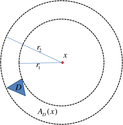
Figure 2: The smallest annulus support $A_{D}(x):=B_{r_{2}}(x)\backslash\overline{B_{r_{1}}(x)}$ centered at the measurement point $x$ with $r_{1}=\inf\{|x-y|\,:\,y\in D\}$ and $r_{2}=\sup\{|x-y|\,:\,y\in D\}$.

To illustrate the asymptotic property of $|(\mathcal{P}^{\ast}_{x}g_{xz})(y)|$ as a function of $\mathbbm{t}$, we refer to Figure 1 where we plot $|(\mathcal{P}^{\ast}_{x}g_{xz})(y)|$ with respect to different $k_{max}$. $|(\mathcal{P}^{\ast}_{x}g_{xz})(y)|$ is a point spread function of $\mathbbm{t}$. In particular, Figure 1 implies that the resolution seems better with larger wave number $k_{max}$.

Now for given $y\in D$ and sampling point $z$, $|(\mathcal{P}^{\ast}_{x}g_{xz})(y)|$ peaks at $\mathbbm{t}=0$, i.e. at sampling point $z$ such that $|x-z|=|x-y|$. In another word, $|(\mathcal{P}^{\ast}_{x}g_{xz})(y)|$ as a function of sampling point $z$ peaks at a sphere centered at $x$ with radius $|x-y|$. Furthermore, turning to $\|\mathcal{P}^{\ast}_{x}g_{xz}\|^{2}_{L^{2}(D)}$ as a function of sampling point $z$, we expect the function $\|\mathcal{P}^{\ast}_{x}g_{xz}\|^{2}_{L^{2}(D)}$ peaks in the smallest annulus support $A_{D}(x):=B_{r_{2}}(x)\backslash\overline{B_{r_{1}}(x)}$ centered at the measurement point $x$ with $r_{1}$ and $r_{2}$ given by (4.17). See Figure 2 for an illustration.

Unfortunately, it is not feasible to compute $\|\mathcal{P}^{\ast}_{x}g_{xz}\|^{2}_{L^{2}(D)}$ directly since $D$ is what we aim to reconstruct. However we are able to relate $\|\mathcal{P}^{\ast}_{x}g_{xz}\|^{2}_{L^{2}(D)}$ to an indicator function given by measurements. Precisely, letting $g=g_{xz}$ in Theorem 4.2 yields that

$$\frac{c_{f}}{4\pi r_{2}}\|\mathcal{P}^{\ast}_{x}g_{xz}\|^{2}_{L^{2}(D)}\leq|(\mathcal{N}_{x}g_{xz},g_{xz})_{L^{2}(K)}|\leq\frac{C_{f}}{4\pi r_{1}}\|\mathcal{P}^{\ast}_{x}g_{xz}\|^{2}_{L^{2}(D)},$$

i.e. $\|\mathcal{P}^{\ast}_{x}g_{xz}\|^{2}_{L^{2}(D)}$ is qualitatively the same as $|(\mathcal{N}_{x}g_{xz},g_{xz})_{L^{2}(K)}|$ for a single measurement point $x$. This implies that the measurement driven function $|(\mathcal{N}_{x}g_{xz},g_{xz})_{L^{2}(K)}|$ peaks in the annulus support $A_{D}(x)$ without the knowledge of $D$. Consequently for all $x\in\Gamma_{L}$, we introduce the indicator function

$$I(z):=\sum_{x\in\Gamma_{L}}\Big{|}(\mathcal{N}_{x}g_{xz},g_{xz})_{L^{2}(K)}\Big{|},\quad z\in{\mathbb{R}}^{3}.$$ (4.23)

To summarize, the indicator function $I(z)$ peaks in the annulus support $A_{D}(x)$ for a single measurement point $x$. With the increase of measurement points, an approximate source support $\bigcap_{x\in\Gamma_{L}}A_{D}(x)$ is expected to be reconstructed by plotting $I(z)$ over a sampling region.

5 Numerical examples

In this section, we present some numerical examples to illustrate the performance of the multi-frequency sampling method.

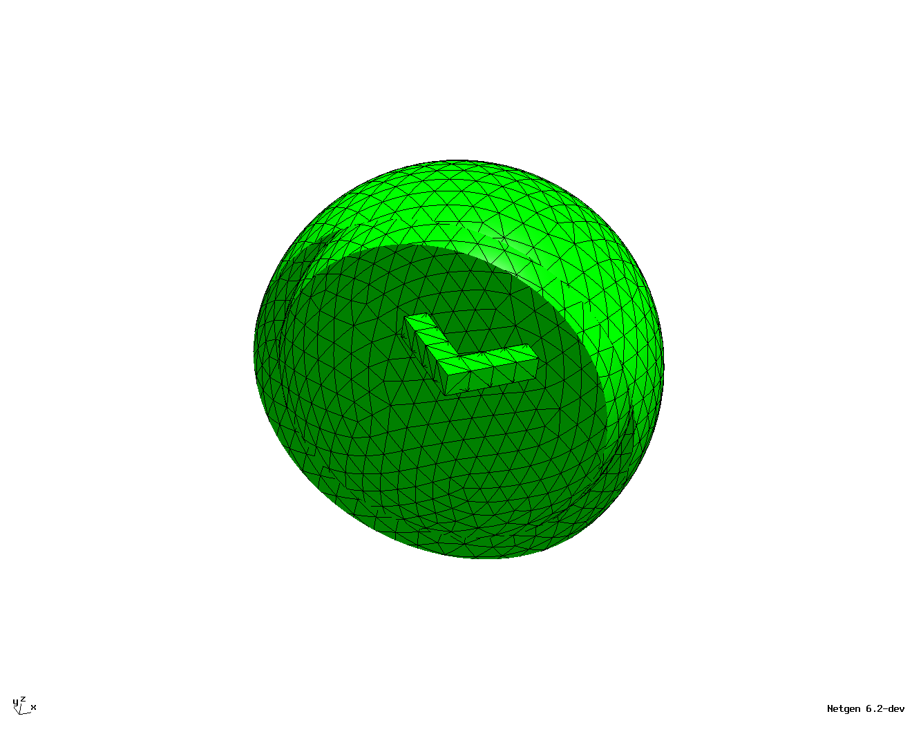
Figure 3: Mesh view of the computational domain.

We generate the synthetic data $u^{s}$ using the finite element computational software Netgen/NGSolve [34]. To be more precise, the computational domain is $\{x:|x|<4\}$ and the measurements are on the sphere $\{x:|x|=3\}$. We apply a radial Perfectly Matched Layer (PML) in the domain $\{x:3.5<|x|<4\}$ and choose PML absorbing coefficient $5i$. See Figure 3 for an illustration. In all of the numerical examples, we apply the second order finite element to solve for the wave field where the source is constant $1$; the mesh size is chosen as $0.5$; the set of wave numbers is $\{k:k=1,2,3,\cdots,11\}$. We further add $5\%$ Gaussian noise to the synthetic data $u^{s}$ to implement the indicator function given by (4.23) in Matlab; for the visualization, we plot $I(z)$ over the sampling region $\{x=(x_{1},x_{2},x_{3}):|x_{j}|<3,\,j=1,2,3\}$ and we always normalize it such that its maximum value is $1$.

We first illustrate the performance of the multi-frequency sampling method with one measurement point. In this example, the measurement point is $(3,0,0)$. The source has support given by a ball

$$\{x:|x_{1}|^{2}+|x_{2}|^{2}+|x_{3}|^{2}<1\}.$$ (5.24)

We plot the exact ball, the three dimensional view of the reconstruction, and its iso-surface view with iso-value $7\times 10^{-1}$ in Figure 4. As expected, the reconstruction is an annulus support of the exact ball.

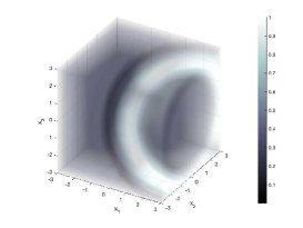
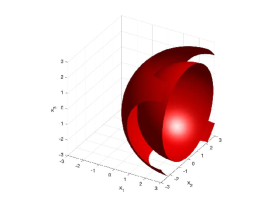
Figure 4: Reconstructions of a ball with one measurement point $(3,0,0)$. Left: 3D view of the exact ball. Middle: 3D view of the reconstruction. Right: iso-surface view of the reconstruction with iso-value $7\times 10^{-1}$.

What may we reconstruct with a little bit more measurements points? Now we still consider the reconstruction of the same ball (5.24) but with $3$ measurement points given by Table 1, where these $3$ measurement points are on the upper half sphere. We plot both the three dimensional reconstruction and its cross-section views in Figure 5. It is observed that the location of ball is clearly indicated with only $3$ measurement points.

$\phi$   $\theta$
————————————————————
-180.0000000000000   45.000000000000000
-90.00000000000000   45.000000000000000
0.0000000000000000   45.000000000000000

Table 1: $3$ measurement points: $(3\sin\theta\cos\phi,3\sin\theta\cos\phi,3\cos\theta)$. Angles are in degrees.

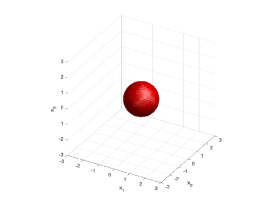
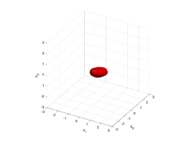
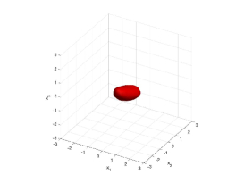
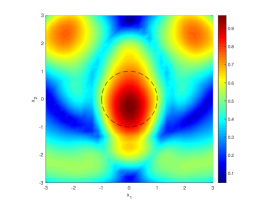
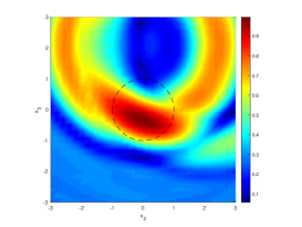
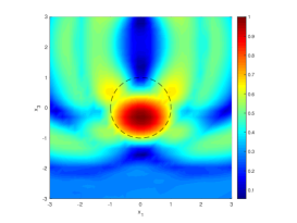
Figure 5: Reconstructions of the ball with $3$ measurement points located on the upper sphere. Top left: exact ball. Top middle and top right: iso-surface view of the reconstruction with iso-values $8.5\times 10^{-1}$ and $8\times 10^{-1}$ respectively. Bottom left: $x_{1}x_{2}$ cross section view of the reconstruction. Bottom middle: $x_{2}x_{3}$ cross section view of the reconstruction. Bottom right: $x_{1}x_{3}$ cross section view of the reconstruction.

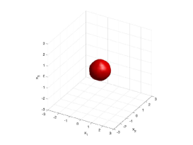
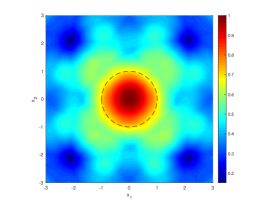
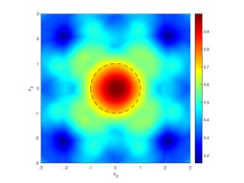
Figure 6: Reconstructions of the ball with $14$ measurement points. Top left: exact ball. Top middle and top right: iso-surface view of the reconstruction with iso-values $7\times 10^{-1}$ and $7.5\times 10^{-1}$ respectively. Bottom left: $x_{1}x_{2}$ cross section view of the reconstruction. Bottom middle: $x_{2}x_{3}$ cross section view of the reconstruction. Bottom right: $x_{1}x_{3}$ cross section view of the reconstruction.

To further shed light on the performance of our imaging algorithm, we consider the case when multiple (but still sparse) measurement points are available all around the source. In the following examples, we consider $14$ measurement points which are roughly equally distributed on the measurement sphere. We remark that only $14\times 11=154$ measurements (in three dimensional space and frequency) are used in this case. The polar coordinates of the $14$ measurement points are given in Table 2.

Figure 6 shows the reconstruction of the ball (5.24) using multiple but sparse measurements. Compared with the reconstruction using $3$ measurement points, it is observed that both the location and shape of the ball are better reconstructed.

$\phi$   $\theta$
————————————————————
0.0000000000000000   90.0000000000000000
180.00000000000000   90.0000000000000000
90.000000000000000   90.0000000000000000
-90.00000000000000   90.0000000000000000
90.000000000000000   0.00000000000000000
90.000000000000000   180.000000000000000
45.000000000000000   54.7356103172453460
45.000000000000000   125.264389682754654
-45.00000000000000   54.7356103172453460
-45.00000000000000   125.264389682754654
135.00000000000000   54.7356103172453460
135.00000000000000   125.264389682754654
-135.0000000000000   54.7356103172453460
-135.0000000000000   125.264389682754654

Table 2: $14$ measurement points: $(r_{m}\sin\theta\cos\phi,r_{m}\sin\theta\cos\phi,r_{m}\cos\theta)$. Angles are in degrees.

We continue to consider a variety of different geometries of the support: a cube (reconstruction in Figure 7) given by

$$\{x=(x_{1},x_{2},x_{3}):|x_{1}|<1,|x_{2}|<1,|x_{3}|<1\},$$

a rounded cylinder (reconstruction in Figure 8) given by

$$\Bigg{\{}x=(x_{1},x_{2},x_{3}):\begin{array}[]{ccc}\sqrt{x_{1}^{2}+x_{2}^{2}}<1&\mbox{ for }&|x_{3}|<1\\ \sqrt{x_{1}^{2}+x_{2}^{2}+(x_{3}-1)^{2}}<1&\mbox{ for }&1<x_{3}<2\\ \sqrt{x_{1}^{2}+x_{2}^{2}+(x_{3}+1)^{2}}<1&\mbox{ for }&-2<x_{3}<-1\end{array}\Bigg{\}},$$

a peanut-shape support (reconstruction in Figure 9) given by

$$\{x=(x_{1},x_{2},x_{3}):\sqrt{(x_{1}-0.5)^{2}+x_{2}^{2}+x_{3}^{2}}<1\mbox{ or }\sqrt{(x_{1}+0.5)^{2}+x_{2}^{2}+x_{3}^{2}}<1\},$$

a L-shape support (reconstruction in Figure 10) given by

$$\{x:-0.5<x_{1}<0,-0.5<x_{2}<1.5,|x_{3}|<0.25\}\cup\{x:0<x_{1}<1.5,-0.5<x_{2}<0,|x_{3}|<0.25\},$$

and two balls (reconstruction in Figure 10) given by

$$\{x:\sqrt{|x_{1}+1|^{2}+|x_{2}|^{2}+|x_{3}|^{2}}<0.5\}\cup\{x:\sqrt{|x_{1}-1|^{2}+|x_{2}|^{2}+|x_{3}|^{2}}<0.5\}.$$

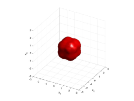
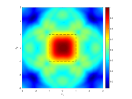
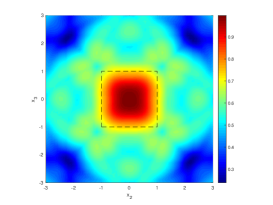
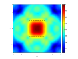
Figure 7: Reconstructions of the cube with $14$ measurement points. Top left: exact cube. Top middle and top right: iso-surface view of the reconstruction with iso-values $7\times 10^{-1}$ and $8\times 10^{-1}$ respectively. Bottom left: $x_{1}x_{2}$ cross section view of the reconstruction. Bottom middle: $x_{2}x_{3}$ cross section view of the reconstruction. Bottom right: $x_{1}x_{3}$ cross section view of the reconstruction.

We observe from the numerical examples that (1) the annulus support of the source can be reconstructed from only one measurement point; (2) the location of a single source can be reconstructed from a few (sparse) measurement points (where we use $3$ measurement points with $11$ different frequencies); (3) both the shape and location of a single source can be well reconstructed from multiple (but sparse) measurement points (where we use $14$ measurement points with $11$ different frequencies) that are roughly equally distributed all around the source. It is also observed that the concave part of the support (see Figure 9 for the peanut and top of Figure 10 for the L-shape) may be reconstructed; (4) the imaging algorithm also works when there are multiple sources (see bottom of Figure 10).

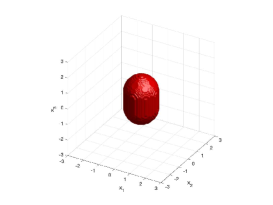
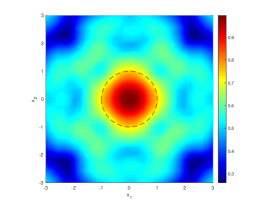
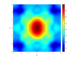
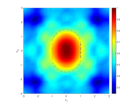
Figure 8: Reconstructions of the rounded cylinder with $14$ measurement points. Top left: exact rounded cylinder . Top middle and top right: iso-surface view of the reconstruction with iso-values $7.5\times 10^{-1}$ and $8\times 10^{-1}$ respectively. Bottom left: $x_{1}x_{2}$ cross section view of the reconstruction. Bottom middle: $x_{2}x_{3}$ cross section view of the reconstruction. Bottom right: $x_{1}x_{3}$ cross section view of the reconstruction.

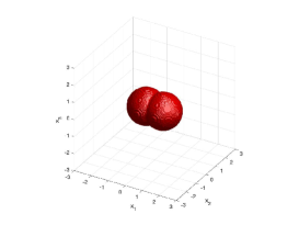
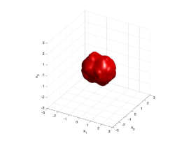
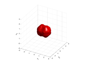
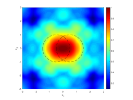
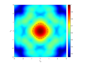
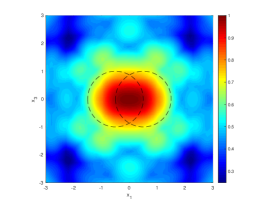
Figure 9: Reconstructions of the peanut with $14$ measurement points. Top left: exact peanut. Top middle and top right: iso-surface view of the reconstruction with iso-values $7.5\times 10^{-1}$ and $8\times 10^{-1}$ respectively. Bottom left: $x_{1}x_{2}$ cross section view of the reconstruction. Bottom middle: $x_{2}x_{3}$ cross section view of the reconstruction. Bottom right: $x_{1}x_{3}$ cross section view of the reconstruction.

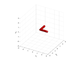
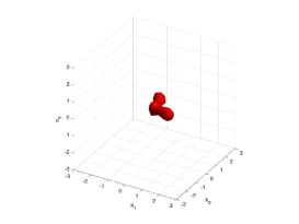
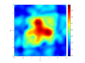
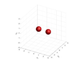
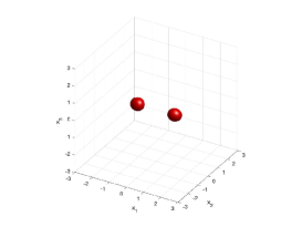
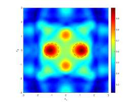
Figure 10: Reconstructions of the L-shape (top) and two balls (bottom) with $14$ measurement points. Left: exact support. Middle: iso-surface view of the reconstruction with iso-values $8.7\times 10^{-1}$ (L-shape) and $8.5\times 10^{-1}$ (two balls). Right: $x_{1}x_{2}$ cross section view of the reconstruction.

6 Appendix: extension to far field measurements

In this appendix we discuss briefly the indicator function defined by the multi-frequency sparse far field measurements. From the asymptotic behavior of Hankel functions, we deduce that the corresponding far field pattern of $u^{s}$ (2.7) has the form

$$u^{\infty}(\hat{x},k)=\int_{D}e^{-ik\hat{x}\cdot\,y}f(y)dy,\quad\hat{x}\in\,S^{2},\,k\in K.$$ (6.25)

We consider the following multi-frequency sparse far field measurements

$$\mathbb{M}_{F}:=\{u^{\infty}(\hat{x},k)\,|\,\hat{x}\in\,\Theta_{L},\,\,k\in K\}$$ (6.26)

with $\Theta_{L}:=\{\pm\hat{x}_{1},\pm\hat{x}_{2},\cdots,\pm\hat{x}_{L}\}\subset S^{2}$.

In view of (6.25), we have

$$u^{\infty}(\hat{x},-k)=u^{\infty}(-\hat{x},k),\quad\hat{x}\in\Theta_{L},\,k\in K.$$

Therefore, the multi-frequency sparse far field measurements $\mathbb{M}_{F}$ (6.26) gives the following data

$$u^{\infty}(\hat{x},k),\quad\hat{x}\in\,\Theta_{L},\,\,k\in[-k_{max},k_{max}]\backslash\{0\}.$$

We define the multi-frequency far field operator $\mathcal{F}_{\hat{x}}:L^{2}(K)\rightarrow L^{2}(K)$ by

$$(\mathcal{F}_{\hat{x}}\phi)(t):=\int_{K}u^{\infty}(\hat{x},t-s)\phi(s)ds,\quad t\in K.$$ (6.27)

The analogous results of Theorem 3.1 and Theorem 4.2 are formulated in the following theorem.

Theorem 6.1.

The far field operator $\mathcal{F}_{\hat{x}}:L^{2}(K)\rightarrow L^{2}(K)$ has a factorization in the form

$$\mathcal{F}_{\hat{x}}=\mathcal{Q}_{\hat{x}}T_{\hat{x}}\mathcal{Q}_{\hat{x}}^{\ast}$$ (6.28)

Here, $\mathcal{Q}_{\hat{x}}:L^{2}(D)\rightarrow L^{2}(K)$ is given by

$$(\mathcal{Q}_{\hat{x}}\psi)(t):=\int_{D}e^{-it\hat{x}\cdot y}\psi(y)dy,\quad t\in K,$$

and its adjoint $\mathcal{Q}_{\hat{x}}^{\ast}:L^{2}(K)\rightarrow L^{2}(D)$ is given by

$$(\mathcal{Q}_{\hat{x}}^{\ast}\phi)(y):=\int_{K}e^{is\hat{x}\cdot y}\phi(s)ds,\quad y\in D.$$

The operator $T_{\hat{x}}:L^{2}(D)\rightarrow L^{2}(D)$ is a multiplication operator given by $T_{\hat{x}}g=fg$, where $f\in L^{2}({\mathbb{R}}^{3})$ is the source with support $D$. Moreover, it holds that

$$c_{f}\|\mathcal{Q}^{\ast}_{x}\phi\|^{2}_{L^{2}(D)}\leq|(\mathcal{F}_{\hat{x}}\phi,\phi)_{L^{2}(K)}|\leq C_{f}\|\mathcal{Q}^{\ast}_{x}\phi\|^{2}_{L^{2}(D)},\quad\forall\phi\in L^{2}(K),\,\hat{x}\in\Theta_{L},$$

where $c_{f}$ and $C_{f}$ are two constants given in (3.9).

Motivated by the results in Theorem 6.1, we introduce the following indicator function

$$I(z):=\sum_{\hat{x}\in\Theta_{L}}\Big{|}(\mathcal{F}_{\hat{x}}\phi_{\hat{x}z},\phi_{\hat{x}z})_{L^{2}(K)}\Big{|},\quad z\in{\mathbb{R}}^{3},$$ (6.29)

where $\phi_{\hat{x}z}\in L^{2}(K)$ is given by

$$\phi_{\hat{x}z}(t)=e^{it\hat{x}\cdot z},\,t\in K.$$ (6.30)

Consequently we have for $y\in D$ that

$$\Big{|}(\mathcal{Q}^{\ast}_{x}\phi_{\hat{x}z})(y)\Big{|}=\Big{|}\int_{K}e^{is\tilde{\mathbbm{t}}}ds\Big{|},\quad\tilde{\mathbbm{t}}=\hat{x}\cdot(z-y),$$ (6.31)

where $\phi_{\hat{x}z}$ is given by (6.30). Similarly, $\Big{|}(\mathcal{Q}^{\ast}_{x}\phi_{\hat{x}z})(y)\Big{|}$ is a point spread function of $\tilde{\mathbbm{t}}$.

We remark that the factorization (6.28) has been derived in [20] where a factorization method is investigated. As can be seen, we have allowed a complex-valued $f$ in the case of far field measurements. We finally remark that the results in this appendix can be directly extended to the two dimensional case.

References

- [1] A. Alzaalig, G. Hu, X. Liu and J. Sun, Fast acoustic source imaging using multi-frequency sparse data, Inverse Problems 36, (2020), 025009.
- [2] H. Ammari, J. Garnier, W. Jing, H. Kang, M. Lim, K. Sølna, and H. Wang, Mathematical and statistical methods for multistatic imaging, volume 2098. Springer, 2013.
- [3] H. Ammari, J. Garnier, V. Jugnon, and H. Kang, Direct reconstruction methods in ultrasound imaging of small anomalies. In Mathematical Modeling in Biomedical Imaging II, pages 31–55. Springer, 2012.
- [4] T. Arens, X. Ji and X. Liu, Inverse electromagnetic obstacle scattering problems with multi-frequency sparse backscattering far field data, Inverse Problems 36, (2020), 105007.
- [5] G. Bao, K. Huang, P. Li and H. Zhao, A direct imaging method for inverse scattering using the Generalized Foldy-Lax formulation, Contemp. Math. 615 (2014), 49-70.
- [6] G. Bao, P. Li, J. Lin and F. Triki, Inverse scattering problems with multifrequencies, Inverse Problems 31, (2015), 093001.
- [7] G. Bao, J. Lin and F. Triki, A multi-frequency inverse source problem, J. Differ. Equ. 249, (2010), 3443-3465.
- [8] G. Bao, J. Lin and F. Triki, Numerical solution of the inverse source problem for the Helmholtz equation with multiple frequency data, Mathematical and statistical methods for imaging, 45-60, Contemp. Math. 548, Amer. Math. Soc., Providence, RI, 2011.
- [9] G. Bao, S. Lu, W. Rundell, and B. Xu, A recursive algorithm for multi-frequency acoustic inverse source problems, SIAM J. Numer. Anal. 53, (2015), 1608-1628.
- [10] N. Bleistein and J. Cohen, Nonuniqueness in the inverse source problem in acoustics and electromagnetics, J. Math. Phys. 18, (1977), 194-201.
- [11] S. Bousba, Y. Guo, X. Wang and L. Li, Identifying multipolar acoustic sources by the direct sampling method, Applicable Analysis 99(5), (2020), 856-879.
- [12] F. Cakoni and D. Colton. A qualitative approach to inverse scattering theory, volume 767. Springer, 2014.
- [13] J. Chen, Z. Chen and G. Huang, Reverse Time Migration for Extended Obstacles: Acoustic Waves, Inverse Problems 29, (2013), 085005.
- [14] D. Colton and A. Kirsch, A simple method for solving inverse scattering problems in the resonance region. Inverse Problems 12 (1996), 383-393.
- [15] D. Colton and R. Kress. Inverse acoustic and electromagnetic scattering theory, volume 93. Springer Nature, 2019.
- [16] A. Devaney, E. Marengo and M. Li, The inverse source problem in nonhomogeneous background media, SIAM J. Appl. Math. 67, (2007), 1353-1378.
- [17] A. Devaney and G. Sherman, Nonuniqueness in inverse source and scattering problems, IEEE Trans. Antennas Propag. 30, (1982), 1034-1037.
- [18] M. Eller and N. Valdivia, Acoustic source identification using multiple frequency information, Inverse Problems 25, (2009), 115005.
- [19] R Griesmaier. Multi-frequency orthogonality sampling for inverse obstacle scattering problems. Inverse Problems 27(8), (2011), 085005.
- [20] R. Griesmaier and C. Schmiedecke, A factorization method for multi-frequency inverse source problems with sparse far field measurements, SIAM J. Imag. Sci. 10, (2017), 2119-2139.
- [21] I Harris, D-L Nguyen. Orthogonality sampling method for the electromagnetic inverse scattering problem. SIAM J. Sci. Comput. 42(3),(2020),722–737.
- [22] K. Ito, B. Jin, and J. Zou, A direct sampling method to an inverse medium scattering problem, Inverse Problems 28, (2012), 025003.
- [23] X. Ji, Reconstruction of multipolar point sources with multifrequency sparse far field data, Inverse Problems 37, (2021), 065015.
- [24] X. Ji and X. Liu, Identification of point like objects with multifrequency sparse data, SIAM J. Sci. Comput. 42(4), (2020), A2325-A2343.
- [25] X. Ji and X. Liu, Inverse electromagnetic source scattering problems with multi-frequency sparse phased and phaseless far field data, SIAM J. Sci. Comput. 41(6), 2019, B1368-B1388.
- [26] X. Ji and X. Liu, Source reconstruction with multi-frequency sparse scattered fields, SIAM J. Appl. Math, 2021, to appear.
- [27] A. Kirsch, Charaterization of the shape of a scattering obstacle using the spectral data of the far field operator, Inverse Problems 14, (1998), 1489–1512.
- [28] A. Kirsch and N. Grinberg. The factorization method for inverse problems. Number 36. Oxford University Press, 2008.
- [29] J. Li, H. Liu and J. Zou, Locating multiple multiscale acoustic scatterers, SIAM Multiscale Model. Simul. 12, (2014), 927–952.
- [30] J. Li and J. Zou, A direct sampling method for inverse scattering using far-field data, Inverse Problems and Imaging 7, (2013), 757-775.
- [31] X. Liu, A novel sampling method for multiple multiscale targets from scattering amplitudes at a fixed frequency, Inverse Problems 33, (2017), 085011.
- [32] X. Liu, S. Meng and B. Zhang, Modified sampling method with near field measurements, arXiv: 2107.00387, 2021.
- [33] R. Potthast, A study on orthogonality sampling, Inverse Problems 26, (2010), 074075.
- [34] J. Schöberl, Netgen an advancing front 2d/3d-mesh generator based on abstract rules, Computing and Visualization in Science 1, (1997), 41–52.
- [35] J. Sylvester and J. Kelly, A scattering support for broadband sparse far field measurements, Inverse Problems 21, (2005), 759-771.
- [36] X. Wang, Y. Guo, D. Zhang and H. Liu, Fourier method for recovering acoustic sources from multi-frequency far-field data, Inverse Problems 33, (2017), 035001.
- [37] D. Zhang, Y. Guo, Fourier method for solving the multi-frequency inverse source problem for the Helmholtz equation, Inverse Problems 31, (2015), 035007.
- [38] D. Zhang, Y. Guo, J. Li and H. Liu, Locating multiple multipolar acoustic sources using the direct sampling method, Commun. Comput. Phys. 25(5), (2019), 1328-1356.