Finite-length effects on beam–plasma instability in collisionless inhomogeneous systems

Abstract

Streaming instability driven by ion flow inside a finite-length collisionless inhomogeneous system is studied with numerical Particle-In-Cell simulations alongside kinetic equations. The inhomogeneous plasma is produced by introducing a cold beam of ions and thermal electrons in the system. In such systems, we observe that the ion sound waves get modified in a stable ion flow due to acoustic wave reflections from the boundary and that it triggers instability. Such phenomena are known to be a hydrodynamic effect. However, there are also signatures of the two-stream type ion sound instability where kinetic resonances are essential. The study is aimed to quantify the effects of the finite-length system on beam–plasma instability and identify wave modes supported by such systems. The outcome of this study is believed to improve design aspect of ion beam sources and provide more control over experimental devices.

Keywords: beam–plasma, ion acoustic instability, finite length

1 Introduction

The streaming instability [1] is one of the oldest and most elementary examples of collective instabilities in plasma physics. Astrophysical plasmas containing small populations of non-thermal particles are susceptible to strong beam–plasma instabilities, leading to redistribution of energy among non-thermal populations. Examples include, but are not limited to, various astrophysical phenomena, such as active galactic nuclei (AGNs) driven beam–plasma instabilities [2, 3, 4], the solar wind [5], pulsar wind outflows [6, 7], shock formation and the associated acceleration of cosmic rays [8, 9].

Moving on to bounded systems, there is a large relevance of beam–plasma interactions in intense heavy ion beams for applications to ion beam–driven high energy density physics (HEDP) and heavy ion fusion (HIF) [10, 11, 12, 13, 12, 13, 14, 15]. Even after several decades of research, the complex nature of the instability continue to draw the attention of the plasma community.

The concept of collective beam–plasma interaction was first introduced by Langmuir [16] in 1925. However, it took a couple of decades to finally realize the potential of this specific phenomena. In 1948, Pierce [17] and later in the same year, Haeff [18] showed the prospects of two-stream instability in signal amplification. In the following year, Bohm and Gross [19, 20] theorized the problem as an electrostatic phenomena in the absence of any magnetic field with kinetic equations. In the past several decades, the problem has been explored by numerous scientists [21, 22, 23, 24, 25, 26, 14, 27, 28, 29, 30, 31, 28, 32].

Most of the mentioned works explicitly deal with electron beams drifting through a plasma. Since the ion beam-induced gas ionization is significantly more rapid than by an electron beam in the same setting, the dynamics is different when an intense ion beam is introduced in a charge-neutralizing background plasma [33, 34, 35]. Similar situations can be found in experiments where plasma beams are introduced inside chambers filled with neutral gas. The beam interacts with the background neutrals and produces a plasma which provides nearly complete charge neutralization of the beam [36, 37]. A complete description of such systems can be described by nonlinear Vlasov-Maxwell equations [38, 39]. However, if we consider the effect of inhomogeneity and intense self-field, it becomes extremely difficult to predict the beam equilibrium, stability, and transport properties. In the present study we are not dealing with relativistic beams, hence self-field can be ignored.

However, the presence of electrically conducting boundaries causes inhomogeneities, and it has a huge impact on the nature of streaming instabilities. Such instabilities appear to be more absolute than convective, i.e., that the waves grow with time but not along spatial position, much alike to in a Pierce diode [40, 17].

In absence of any external or self-generated magnetic field, the most significant process among the collective processes associated with an ion beam and a charge-neutralizing background plasma is electrostatic electron–ion two-stream instability [41, 42, 43]. The source of free energy to drive the classical two-stream instability comes from the relative streaming of beam electrons through the charge-neutralizing background plasma. The nature of such beam–plasma interactions is found to be highly dependent on the system length. In infinite systems, for a simplest case where collisions are neglected, and the ions do not have any drift velocity (streaming is only due to electron drift), the spatial growth rate of such waves become theoretically infinite at a certain frequency near the electron plasma frequency, meaning the instability is absolute. For finite-length systems with small drift velocities for background ions, the wave appears to grow spatially, for waves at frequencies of the order of the ion plasma frequency instead [17]. Inclusion of collisions and increasing temperature certainly affects the growth and effectively bounds the amplification rate [44, 45]. However, it is worth mentioning that the present work does not consider any effects from collisions.

In systems where ion beams stream through thermal electrons, in relatively cold plasmas, the spatial growth of waves are found strongest at a certain frequencies near the electron plasma frequency [46, 47, 48]. However, it can also be of the order of the ion plasma frequency, provided the unperturbed beam velocity is very small compared to the average thermal velocity of background plasma electrons [49, 50]. Such non-equilibrium systems may also exhibit excitation of ion sound waves when the relative velocity between the ion stream and background electrons exceeds the ion sound velocity ($\Delta v>c_{s}$) [51, 52, 53].

There are limitless implications of instabilities due to streaming ion beams such as in electric propulsion system [54], plasma diodes [55, 56], double layers [57, 58], and even for the sheath region at plasma–material boundaries [59]. Depending on the triggering mechanism, it can either lead to hydrodynamic instabilities such as ion sound instability [54] or kinetic instabilities like the two-stream instability [41, 42, 43].

In our present work, we present a collective picture of instabilities due to an ion beam streaming through thermal plasma, the beam being injected from one of the boundaries in a bounded system. This may for instance be due to an ion-emitting source in a plasma device. In complex systems such as ours, the hardest part is to address the effect of inhomogeneity due to the presence of the boundary in the system. The ideal theory of the beam–plasma instability does not stand well when we bring all the factors into the picture. In presence of inhomogeneity, we have found the fast wave modes appear to be drastically different as compared to the homogeneous cases. Whereas, slow wave modes become of more ion acoustic nature far away from the source. There are several studies associated with beam–plasma instability that address inhomogeneous media [60, 61, 62, 63, 64, 65]. Apart from the classical papers by Takakura and Shibahashi [64], Magelssen and Smith [65], the recent works by Shalaby et al. [60, 61] are worth mentioning in this regard. However, the above-mentioned papers address the inhomogeneity assuming the electron/positron beams are streaming within inhomogenous media and do not cover the exact situation we are dealing with at present. The most relevant work with the closest proximity to ours would be the work by Rapson et al. [51], where they studied the effect of boundaries on the ion acoustic beam–plasma instability. The present paper stands out in two different aspects. First, we assume a cold ion beam streaming through thermal electrons. Secondly, the inhomogeneity in the system arises naturally due to the presence of conducting surfaces in both ends.

One of the important aspect of such studies is to understand the plasma waves excited in ionospheric simulators. The ionospheric simulators are plasma chambers equipped with ion source of high mach number flow in a neutralizing environment. These chambers can reproduce ionospheric plasma conditions to test electrical probes before they are used in space missions. The present paper aims to explain the instabilities found in such devices in order to improve the control environment for space probes.

The paper is organized as follows. In section II, dispersion theory for homogeneous and inhomogeneous media are presented followed by numerical methods and simulation setup details in section III. Results and relevant discussions are provided in section IV. Finally, in section V the work is summarized and concluded.

2 Analytical theories of wave dispersion in beam–plasma systems

2.1 Dispersion theory for homogeneous media

For the ion beam-driven ion acoustic instability, the dispersion relation for the simplest one-dimensional case takes the following form [66, 67, 68],

$$\epsilon(k,\omega)=1+\frac{e^{2}}{\epsilon_{0}m_{e}k}\bigintsss_{u}\frac{\partial F_{0e}/\partial u}{\omega-ku}du,$$ (1)

$$+\frac{e^{2}}{\epsilon_{0}m_{i}k}\bigintsss_{u}\frac{\partial F_{0ib}/\partial u}{\omega-ku}du=0$$

where, $m_{e}$ and $m_{i}$ are the mass of electron and ion respectively. $~{}\epsilon_{0}$ and $e$ represents the permittivity of free space, and the elementary charge. $k$ stands for the wave number and $\omega$ is the wave frequency. $F_{0e}$, and $F_{0ib}$ are the phase space distributions of background thermal electrons, and cold beam ions respectively.

Now for a wave with a phase velocity $\omega/k$ much less than electron thermal velocity but larger than ion thermal velocity we can assume $\omega\ll ku$ for background electron. Hence, the second term in the right hand side of eq. 1 can be approximated as,

$$\frac{e^{2}}{\epsilon_{0}m_{e}k}\bigintsss_{u}\frac{\partial F_{0e}/\partial u}{\omega-ku}du=\frac{\omega_{pe}^{2}}{k^{2}}\frac{m_{e}}{T_{e}}=\frac{1}{k^{2}\lambda_{D}^{2}},$$ (2)

considering that background electrons are Maxwellian with a temperature $T_{e}$ (in electron-volts),

$$F_{0e}(u)=\frac{n_{e}}{\left(2\pi T_{e}/m_{e}\right)^{1/2}}\exp\left(-\frac{m_{e}u^{2}}{2T_{e}}\right).$$

The electron plasma frequency is $\omega_{pe}=\sqrt{\frac{n_{e}e^{2}}{\epsilon_{0}m_{e}}}$, and the Debye length is $\lambda_{D}=\sqrt{\frac{\epsilon_{0}k_{b}T_{e}}{n_{e}e^{2}}}$, $n_{e}$ is the electron density and $k_{b}$ represents Boltzmann’s constant.

For the ion beam contribution, we can not consider $\omega\gg ku$, as the beam velocity ($v_{b}$) is comparable to the wave velocity. Hence, the last term can be approximated as,

$$\frac{e^{2}}{\epsilon_{0}m_{i}k}\bigintsss_{u}\frac{\partial F_{0ib}/\partial u}{\omega-ku}du=-\frac{\omega_{pi}^{2}}{{(\omega-kv_{b})}^{2}},$$ (3)

where $\omega_{pi}=\sqrt{\frac{n_{i}e^{2}}{\epsilon_{0}m_{i}}}$ is the ion plasma frequency. Now, using, eqs. 2 to 3 in eq. 1 we get,

$$\epsilon(k,\omega)=1+\frac{1}{k^{2}\lambda_{D}^{2}}-\frac{\omega_{pi}^{2}}{{(\omega-kv_{b})}^{2}}=0$$ (4)

The first two terms represent the bulk plasma oscillations and the last term comes due to the presence of a beam. The frequencies of the excited wave modes are of the order of ion time scales ($\omega_{pi}$). The normalized eq. 4 takes the following form,

$$\epsilon(\tilde{k},\tilde{\omega})=1+\frac{1}{\tilde{k}^{2}}-\frac{1}{{(\tilde{\omega}-\tilde{k}\tilde{v}_{b})}^{2}}=0$$ (5)

$$\tilde{k}=k\lambda_{D},~{}~{}\tilde{\omega}=\frac{\omega}{\omega_{pi}},~{}~{}\tilde{v}_{b}=v_{b}/C_{s}$$

where, $\tilde{k}$, $\tilde{\omega}$, and $\tilde{v}_{b}$ are the normalized wave number, normalized plasma frequency, and normalized beam velocity. $C_{s}=\sqrt{T_{e}/m_{i}}$ is the ion acoustic speed.

Our aim is to use the dispersion theory to draw conclusion for complex cases from PIC simulations where we expect to have kinetic effects. Such comparison will help in isolating the effects from kinetic properties of beam–plasma systems and to assess the finite-length effects on such systems.

2.2 Dispersion theory for beam–plasma in inhomogeneous medium

As stated in the introduction, the formalism for estimating the growth of a beam–plasma instability in an inhomogeneous medium is naturally complicated as there are many factors in play. In this section, we adopt the formalism developed by Shalaby et al. [60] to estimate the growth in such a system. In the present case, the first-order (linearized) Vlasov-Maxwell equations can be re-written as an eigenvalue problem as:

$$\frac{e^{2}}{\epsilon_{0}m_{e}k}\bigintsss_{u}\bigintsss_{k^{\prime}}\frac{\partial F_{0e}(k^{\prime},u)/\partial u}{\omega-ku}E_{1}\left(k-k^{\prime},\omega\right)dk^{\prime}du$$ (6)

$$+\bigg{[}1+\frac{e^{2}}{\epsilon_{0}m_{i}k}\bigintsss_{u}\frac{\partial F_{0ib}/\partial u}{\omega-ku}du\bigg{]}E_{1}(k,\omega)=0$$

where, $E_{1}$ is the first-order perturbation in the electric field. The important difference between eq. 6 and eq. 1 is the inhomogeneity introduced in background electron term. $F_{0e}$ is the equilibrium phase space distribution of thermal electron of the following form,

$$F_{0e}(x,u)=n_{e}(x)F_{0e}(u)$$ (7)

Assuming the plasma inhomogeneity to be of quadratic nature allows us to arrive at a particular, analytic solution. The background density for electrons can then be expressed as,

$$n_{e}(x)=n_{e0}(1+\xi x^{2});~{}\xi\leq 0$$ (8)

where $\xi$ is the inhomogeneity factor and has a dimension of inverse length squared. Using eq. 8 in eq. 7 and taking the Fourier transform, the equation becomes,

$$F_{0e}\left(k^{\prime},u\right)=n_{e0}\left[\delta\left(k^{\prime}\right)-\xi\delta^{\prime\prime}\left(k^{\prime}\right)\right]F_{0e}(u)$$ (9)

Using eq. 9 in the first term of eq. 6 and integrating over $k^{\prime}$ gives,

$$\left[\frac{e^{2}}{\epsilon_{0}m_{e}k}\bigintsss_{u}\frac{\partial F_{0e}/\partial u}{\omega-ku}du\right](1-\xi\partial_{k}^{2})E_{1}(k,\omega)$$ (10)

Splitting eq. 10 and simplify we obtain,

$$\left[\frac{e^{2}}{\epsilon_{0}m_{e}k}\bigintsss_{u}\frac{\partial F_{0e}/\partial u}{\omega-ku}du\right]E_{1}(k,\omega)$$ (11)

$$-\xi\left[\frac{e^{2}}{\epsilon_{0}m_{e}k}\bigintsss_{u}\frac{\partial F_{0e}/\partial u}{\omega-ku}du\right]\partial_{k}^{2}E_{1}(k,\omega)$$

Now, using eq. 2, the integrals in eq. 11 can be rewritten as,

$$\left(\frac{1}{k^{2}\lambda_{D}^{2}}\right)E_{1}(k,\omega)-\xi\left(\frac{1}{k^{2}\lambda_{D}^{2}}\right)\partial_{k}^{2}E_{1}(k,\omega)$$ (12)

Using eq. 3 and eq. 12, we can rewrite eq. 6 as,

$$\epsilon(k,\omega)=\left(\frac{1}{k^{2}\lambda_{D}^{2}}\right)E_{1}(k,\omega)$$ (13)

$$-\xi\left(\frac{1}{k^{2}\lambda_{D}^{2}}\right)\partial_{k}^{2}E_{1}(k,\omega)$$

$$+\left[1-\frac{\omega_{pi}^{2}}{{(\omega-kv_{b})}^{2}}\right]E_{1}(k,\omega)=0$$

Now, eq. 13 can be rewritten as,

$$-\frac{\xi}{k^{2}\lambda_{D}^{2}}\partial_{k}^{2}E_{1}+\Bigg{[}1-\frac{\omega_{pi}^{2}}{{(\omega-kv_{b})}^{2}}\Bigg{]}E_{1}+\frac{1}{k^{2}\lambda_{D}^{2}}E_{1}=0$$ (14)

Similar to eq. 5, if we write eq. 14 using normalized expressions for $\omega$, $k$, and $\xi$,

$$\frac{-\tilde{\xi}}{\tilde{k}^{2}}\partial_{\tilde{k}}^{2}E_{1}+\left[1-\frac{1}{{(\tilde{\omega}-\tilde{k}\tilde{v_{b}})}^{2}}\right]E_{1}+\frac{1}{\tilde{k}^{2}}E_{1}=0$$ (15)

where, $\tilde{\xi}=\xi\lambda_{D}^{2}$, and $E_{1}$ is a function of $\tilde{k},\tilde{\omega}$.

Now, let’s introduce $A=\tilde{\xi}$ and $B(\tilde{k})=\left[1-\frac{1}{{(\tilde{\omega}-\tilde{k}\tilde{v_{b}})}^{2}}\right]$. If we Taylor expand $B$ to the zeroth order around $\tilde{k}=0$ such that it becomes independent of $\tilde{k}$, i.e., $B\approx 1-\frac{1}{\tilde{\omega}}$, then the above equation can be written as the Weber differential equation. In the small perturbation limit to the potential by the beam, [69, 70], the solution for first-order perturbation in the E-field can be written as,

$$E_{1}(\tilde{k},\tilde{\omega})=C_{1}D_{-\frac{1}{2}\left(\frac{1}{\sqrt{A}\sqrt{B}}+1\right)}\left(\frac{\sqrt{2}\sqrt[4]{B}\tilde{k}}{\sqrt[4]{A}}\right)$$ (16)

$$+C_{2}D_{\frac{1}{2}\left(\frac{1}{\sqrt{A}\sqrt{B}}-1\right)}\left(\frac{i\sqrt{2}\sqrt[4]{B}\tilde{k}}{\sqrt[4]{A}}\right)$$

where, $D_{\nu}$ is the parabolic cylinder function [71, 69, 72]. A more general form of eq. 16 can be written as,

$$E_{1}(\tilde{k},\tilde{\omega})=C_{1}D_{\nu}\left(y\right)+C_{2}D_{-\nu-1}\left(iy\right),~{}\nu\in\mathbb{R}$$ (17)

where, $y=\left(\sqrt{2}\sqrt[4]{\frac{B}{A}}\tilde{k}\right)$, and $C_{1,2}$ are integration constants. Again we make use of the zeroth-order approximation of $B$, so that $y$ becomes linear in $\tilde{k}$. Then, $y\approx\left(\sqrt{2}\sqrt[4]{\frac{1-1/\tilde{\omega}^{2}}{A}}\tilde{k}\right)$.

Considering the solution to be finite as $|k|\to\infty$, the coefficient of the imaginary solution has to be zero. Hence, eq. 17 takes the following form,

$$E_{1}(\tilde{k},\tilde{\omega})=C_{\nu}D_{\nu}\left(y\right),~{}\nu\in\mathbb{R}$$ (18)

If we consider $\nu$ to be a non-negative integer $n$, then $D_{\nu}$ can be rewritten as,

$$D_{n}(y)=2^{-n/2}e^{-y^{2}/4}H_{n}\left(\frac{y}{\sqrt{2}}\right),~{}n\in\mathbb{N}_{0}$$ (19)

where $H_{n}$ is a Hermite polynomial. Now, using eq. 19, the a general expression for eq. 16, considering $n\in\mathbb{N}_{0}$, can be written as a solution for a quantum harmonic oscillator,

$$E_{1}(\tilde{k},\tilde{\omega})=C_{n}e^{-y^{2}/4}H_{n}\left(\frac{y}{\sqrt{2}}\right)$$ (20)

A more general approach towards the problem would be to consider eq. 18 and substituting it in eq. 15. In evaluating $\partial_{\tilde{k}}^{2}D_{\nu}(y)$, one should remember that both $\nu$ and $y$ are functions of $\tilde{k}$, and that some simplification is necessary in order to eliminate the common factor $C_{\nu}D_{\nu}(y)$. Again using the zeroth order Taylor expansion of $B$ around $\tilde{k}=0$, we arrive at,

$$\frac{\sqrt{\tilde{\xi}}}{\tilde{k}^{2}}\sqrt{1-1/\tilde{\omega}^{2}}\Bigg{(}2\nu+1\Bigg{)}$$ (21)

$$+\left[\frac{1}{\tilde{k}^{2}}+\frac{1}{\tilde{\omega}^{2}}-\frac{1}{{(\tilde{\omega}-\tilde{k}\tilde{v_{b}})}^{2}}\right]=0$$

It is important that, unlike in some other applications of the Weber differential equation, $\nu$ is not an independently varying parameter, but depends in a strict way on $\tilde{\omega}$ and $\tilde{\xi}$. Substituting the value of $\nu$ in eq. 20 we get,

$$-2\frac{\sqrt{\tilde{\xi}}}{\tilde{k}^{2}}\sqrt{1-\frac{1}{\tilde{\omega}^{2}}}+\frac{1}{\tilde{\omega}^{2}}+\frac{1}{{(\tilde{\omega}-\tilde{k}\tilde{v_{b}})}^{2}}=0$$ (22)

One might expect that as $\xi\rightarrow 0$, the expression should reduce to eq. 5 (the homogeneous case). However, because of the Taylor approximations this is not the case, and eq. 5 would naturally be the more accurate expression for the homogeneous case. For small values of $\tilde{k}$, however, (near the origin of the dispersion plots to be shown later), the above expression should be accurate.

3 Numerical method and simulation setup

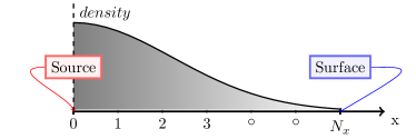
Figure 1: Schematic of the simulation model

Kinetic simulations are performed with a 2D3V particle-in-cell (PIC) code, XOOPIC (X11-based Object-Oriented Particle-In-Cell) [73]. The model uses two-dimensional Cartesian geometry to represent a plasma system of variable lengths (see fig. 1). The system is considered periodic in y-direction, which essentially reduces the problem to 1D. A plasma source is introduced in the system from the left. The source is modeled such that ions can have different drift velocities. We have considered ions to be cold ($0.01~{}eV$) with drift velocities ranging from $0.1~{}eV$ to $7.5~{}eV$ which in normalized units is equivalent to $\sim 0.489~{}C_{s}$ to $\sim 4.242~{}C_{s}$ and electrons are introduced with only the thermal component at $0.5~{}eV$. The specific values for system parameters have been adopted from the ionospheric environment simulator system at the University of Oslo, Norway. The plasma is considered unmagnetized and self-generated magnetic field is ignored assuming small current values. The plasma density has been taken as $\approx 10^{13}~{}m^{-3}$ and hydrogen has been considered to be the ion species. Field quantities are dumped periodically to measure temporal growth rate of instability as well as the dispersion of the electrostatic waves using Fourier transformation. In all of the case studies, the cell size ($\Delta x$) is taken as the Debye length ($\lambda_{D}$) of the respective system. For time step, we used $\Delta t\omega_{pe}=0.02$, which is sufficiently small to resolve electron plasma oscillations. In order to study finite-length effects, the system length has been varied from $512~{}\lambda_{D}$ to $2048~{}\lambda_{D}$. For periodic cases, the system length is set at $1024~{}\lambda_{D}$. Note that even in the periodic case, wavelengths longer than the system length (small $\tilde{k}$) are not supported. Our choice results in a good resolution of $\tilde{k}$.

Although the code takes unnormalized input, the outputs have been normalized with relevant quantities to highlight the physical scaling. Ion velocities are normalized with ion sound speed ($C_{s}$), whereas electron velocities are normalized with the electron thermal velocity ($v_{th}$). Normalized ion and electron velocities are expressed as $\tilde{v}_{i}$, and $\tilde{v}_{e}$ respectively. Time is normalized with inverse of ion plasma frequency ($\omega_{pi}$) and denoted as $\tau$. Lengths are normalized with electron Debye length ($\lambda_{D}$), and expressed as $\tilde{x}$. Lastly, kinetic energies ($\varepsilon_{i,e}$) are normalized by the thermal energy ($\varepsilon_{i,e}^{th}$) of the respective species.

4 Results and discussions

The key objective of this work was to establish the role of ion flow in the development of streaming instabilities in inhomogeneous bounded systems. It is expected that bounded systems act very differently as compared to periodic systems and theoretical justifications for such cases are hard to establish. To understand the parameter regime excluding any effect from boundary, first, we have investigated the analytical theory for homogeneous and inhomogeneous media. We then continue with the kinetic simulations for similar systems. We remark that the simulations are different from the analytical derivations in that the inhomogeneity arises naturally as a consequence of ions being emitted from a source on the left, as in experimental devices, whereas the analytical theory prescribes a quadratic dependence. The two cases, however, show qualitative similarities.

The ion acoustic waves resemble sound waves in neutral media and are primarily compressional. These oscillations are one of the fundamental eigenmodes of finite temperature plasmas. The restoring force for the oscillation is provided by the electron compressibility (pressure) and is transferred to ions through the electric field while the inertia is provided by ions [74]. Regardless of the nature, electrostatic forces also play an important role in the excitation of waves. Due to the smaller mass, electrons are pushed away from high pressure regions faster than ions, resulting in a net positive charge. Such differences are limited to Debye scales, which can also be seen from the second term of eq. 5.

Reviewing the applicability of homogeneous dispersion theory to the present scenario comes with several aspects. For sake of simplicity, we have even dropped any contribution from pressure assuming zero temperature (i.e. $v_{th}\ll v_{b}$) for the beam. In the later part of the paper, it can be seen how such approximation helped us to capture the wave modes.

4.1 Results from kinetic dispersion theory

4.1.1 Waves in infinite homogeneous systems

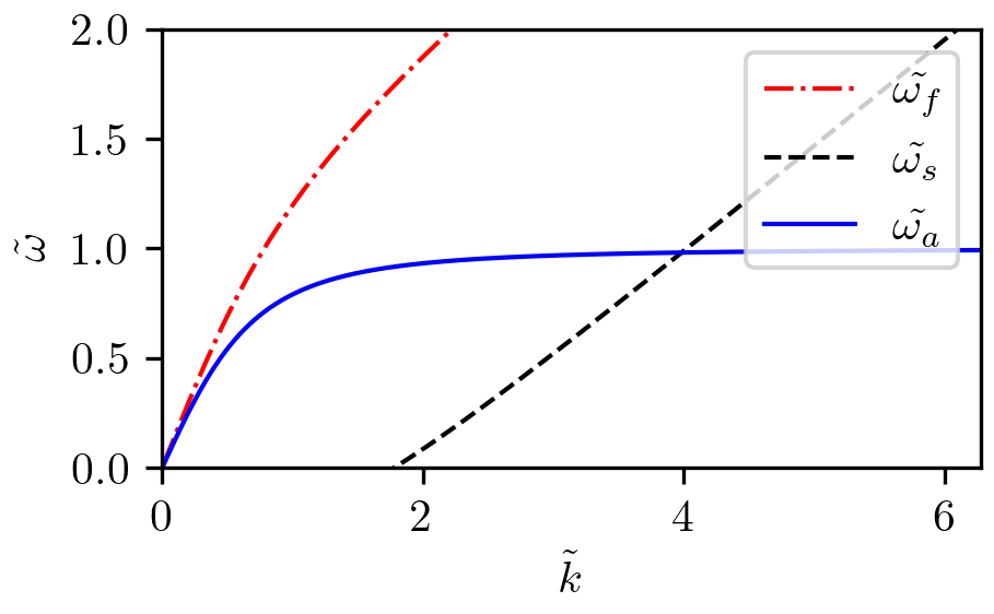
(a)

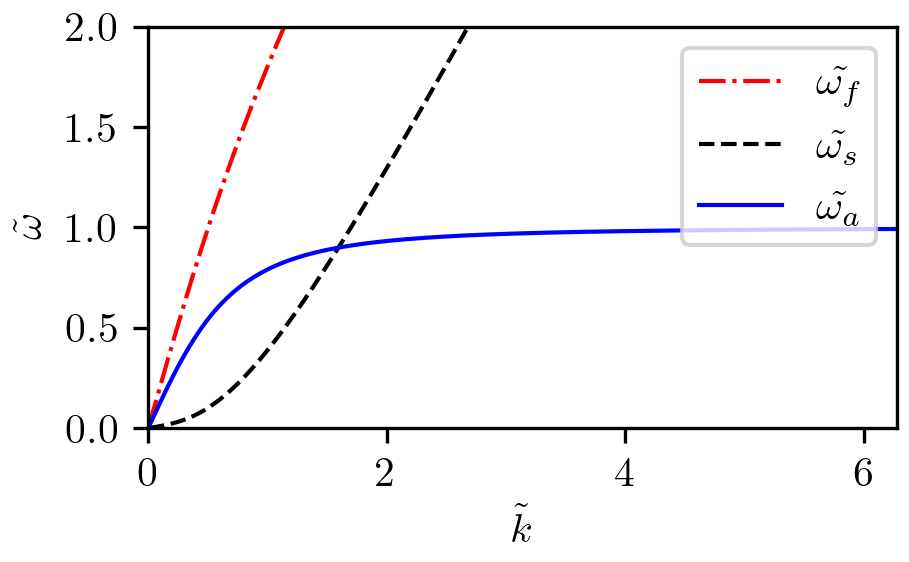
(b)

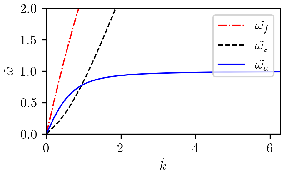
(c)

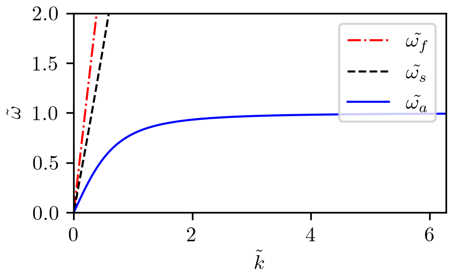
(d)

Figure 2: Analytic solutions for the periodic system with (a) $\tilde{v_{b}}=0.489$, (b) $\tilde{v_{b}}=1.095$, (c) $\tilde{v_{b}}=1.549$, and (d) $\tilde{v_{b}}=4.242$.

Solving eq. 5 for $\tilde{\omega}$ would give four different roots, of which the complex roots are the indication of unstable growth. For the given set of parameters, plasma can exhibit two different modes of oscillations; fast beam mode ($\tilde{\omega_{f}}$), slow beam mode ($\tilde{\omega_{s}}$) for ions. The acoustic mode ($\tilde{\omega_{a}}$) is included as a reference to a more general case in large wavelength limit, $\lambda_{D}\ll L$ (system length). From fig. 2, we can see how the fast wave modes and slow wave modes get affected due the change in ion beam velocity. For subsonic and sonic beam velocity, the fast wave mode seems to approach the acoustic branch at lower $\tilde{k}$ (fig. 2a and fig. 2b). Whereas for supersonic case (fig. 2c), slow wave mode appears to act in the same way. Increasing the beam velocity further, both the modes start to merge and move further away from the acoustic branch.

4.1.2 Waves in finite inhomogeneous systems

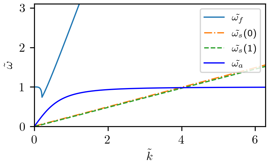
(a)

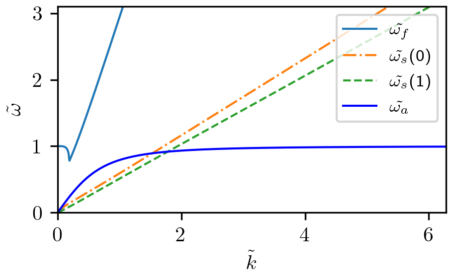
(b)

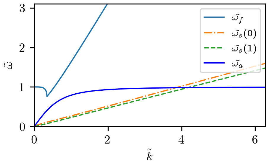
(c)

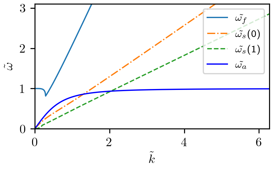
(d)

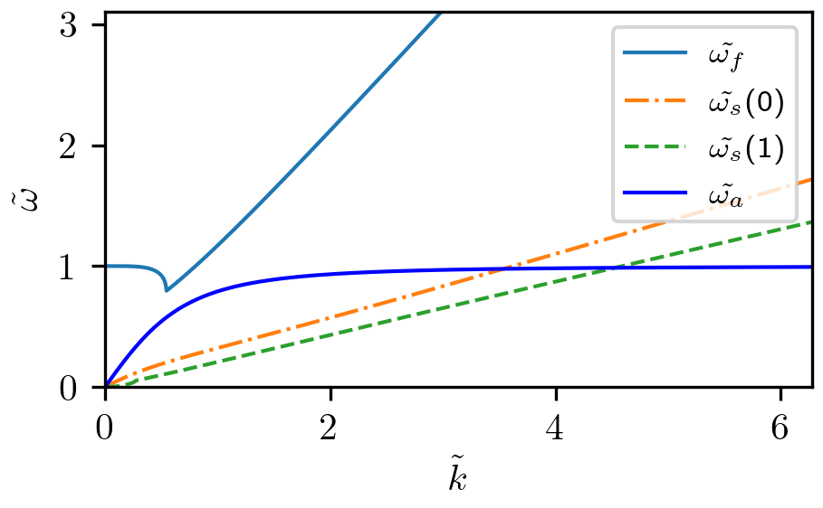
(e)

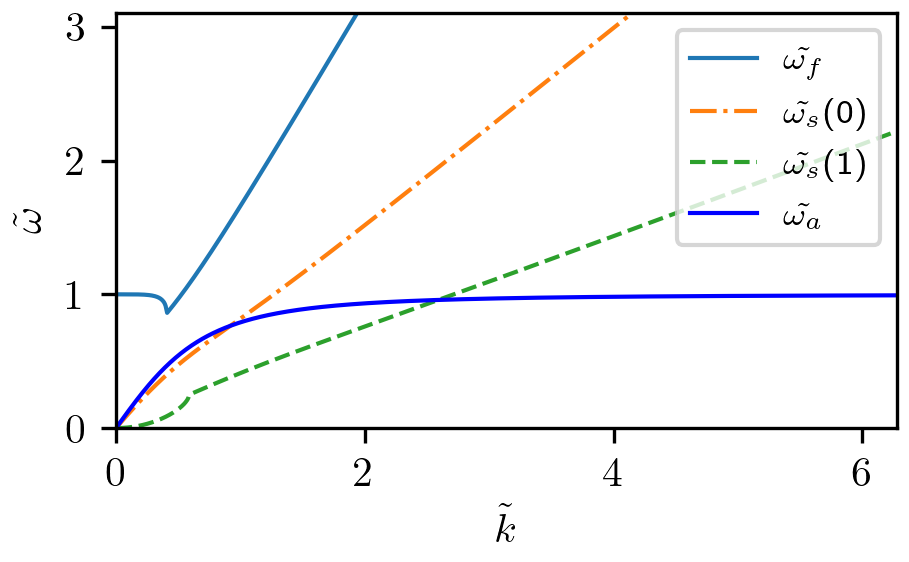
(f)

Figure 3: Analytic solutions for the inhomogeneous bounded system from eq. 22 with (a) $\tilde{v_{b}}=0.489$, $\tilde{\xi}=-0.01$, (b) $\tilde{v_{b}}=1.095$, $\tilde{\xi}=-0.01$, (c) $\tilde{v_{b}}=0.489$, $\tilde{\xi}=-0.1$, (d) $\tilde{v_{b}}=1.095$, $\tilde{\xi}=-0.1$, (e) $\tilde{v_{b}}=0.489$, $\tilde{\xi}=-1.0$, (f) $\tilde{v_{b}}=1.095$, $\tilde{\xi}=-1.0$. Three different wave modes are denoted as $\tilde{\omega_{f}}$ (fast beam mode), $\tilde{\omega_{s}}$ (slow beam mode), and $\tilde{\omega_{a}}$ (acoustic mode). Acoustic wave mode (solid blue curve) is derived using analytical expression separately for comparison.

Figure 3 shows the solutions for different wave modes with subsonic, and sonic, beam velocities in presence of inhomogeneity in the system. Upon expansion eq. 22 becomes an octic or polynomial of degree eight. Further simplification and solving for $\tilde{\omega}$ provides us three sets of solutions. The fast wave mode ($\tilde{\omega_{f}}$) seems to be independent of $\tilde{k}$ at low values, and with increasing inhomogeneity the group velocity (i.e. slope of the curves) $v_{g}$ appears to get smaller. The slow wave mode ($\tilde{\omega_{s}}$) has two branches (noted as $\tilde{\omega_{s}}(0)$ and $\tilde{\omega_{s}}(1)$ in fig. 3) and the group velocity of each branch has shown strong dependence on inhomogeneity. For subsonic case, the both the branches of slow wave modes appear to be merged for small inhomogeneity. However, for sonic case they remain separated even for small inhomogeneity. The difference in group velocity due to inhomogeneity has larger impact when the ion beam moves to sonic range. At low $\tilde{k}$ values, strong inhomogeneity allows the slow wave mode to have a growth similar to acoustic wave.

In presence of inhomogeneity, the group velocity of fast wave mode becomes negative at $\tilde{k}<1$, which indicates the presence of backward moving wave. As the inhomogeneity gets stronger the point of reflection moves away from the source. This observation seems to have no difference as beam goes sonic.

While solving eq. 22, for simplicity we assumed our solution to be valid near $\tilde{k}=0$. We expect to observe difference when we compare the analytical results with simulations. In the remainder of this paper we will investigate how the analytical solutions could explain the results from kinetic simulations.

4.2 Results from kinetic simulations

4.2.1 Waves in infinite homogeneous systems

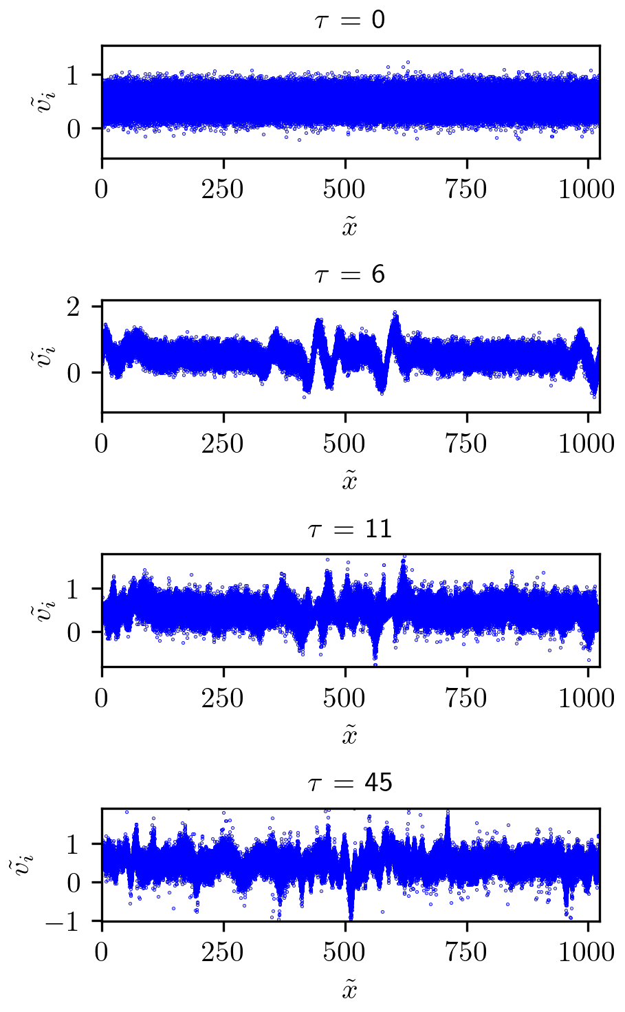
Figure 4: Phase space of ions at different stages of simulation for the periodic system with $\tilde{v_{b}}=0.489$. Times are mentioned inside each panel.

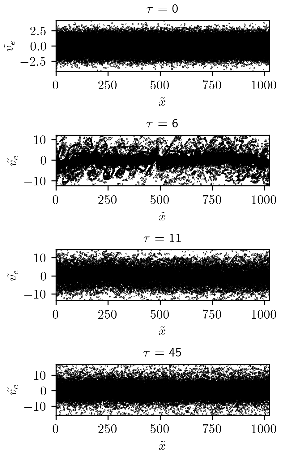
Figure 5: Phase space of electrons at different stages of simulation for the periodic system with $\tilde{v_{b}}=0.489$. Times are mentioned inside each panel.

Figure 4 and fig. 5 represent the phase space of the periodic system with subsonic beam velocity ($\tilde{v_{b}}=0.489$). In the absence of collisions, the plasma consists mostly of the cold beam ions and thermal electrons (if we ignore the small thermal population of ions). Over time the electrons gain energy due to the Coulomb interaction with the beam ions. Streaming between beam ions and thermal electrons leads to the excitement of a low-frequency wave. It results in band formation across the plasma (see fig. 4 and fig. 5). Such complex phase space structures can be as big as hundreds of Debye lengths, as seen in the same figures at $\tau=6$. Afterward, as the instability grows with time and the system approaches thermal equilibrium, these structures break into smaller forms with the size of tens of Debye lengths.

Figure 6 shows the evolution of average kinetic energy of individual species normalized by the thermal energy of the respective species. The wave excitation can be observed approximately at $\tau=4$ (4 ion plasma periods), and the energy growth hits the maximum value at $\tau\sim 6$. If we closely compare the energy growth in the system with the particle phase space, it becomes clear how after $\sim 6$ ion plasma period, the phase space mixes and ends up with thermal/chaotic motion.

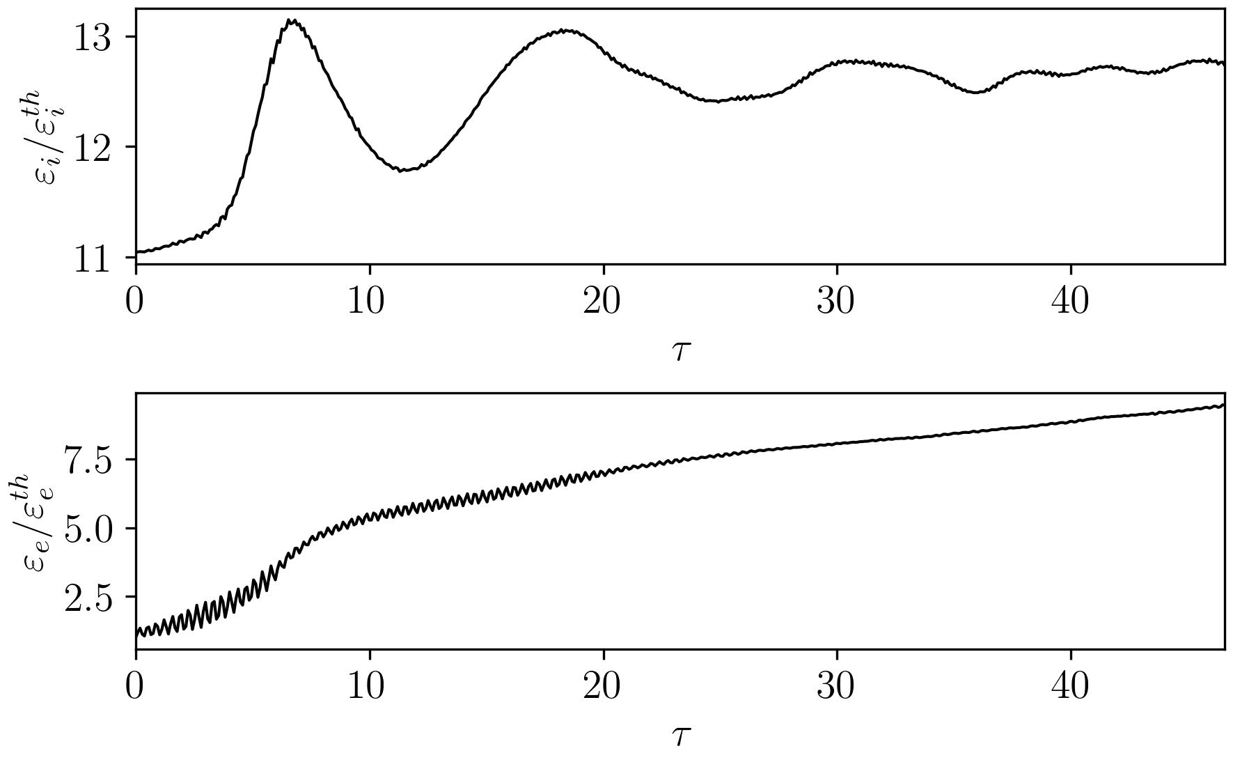
Figure 6: Evolution of the average kinetic energy of ions (top) and electrons (bottom) for the periodic system with $\tilde{v_{b}}=0.489$. The average kinetic energy of individual species is normalized by thermal energy of the respective species.

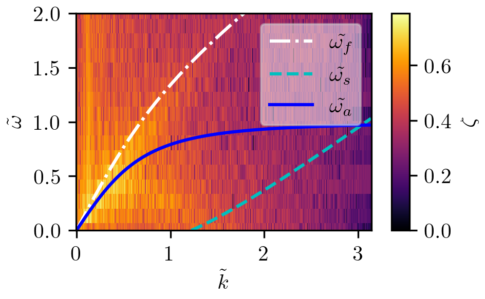
Figure 7: Plasma dispersion from the electric field for the periodic system with $\tilde{v_{b}}=0.489$ along with numerical solutions for eq. 6. The color-map corresponds to the normalized electric field ($\zeta$). The e-field has been normalized with maximum e-field value in the system.

Figure 7 gives a justification for the complex structures visible in fig. 4. In regard to the analytical fluid dispersion curves of the system, we can see that the fast wave mode ($\tilde{\omega_{f}}$) is dominates over the other branches and couples with the ion acoustic branch ($\tilde{\omega_{a}}$). More importantly, the excited wave modes in the system remain within the expected values predicted by the dispersion theory for homogeneous system. However, for subsonic beam velocity, no signature of slow wave mode ($\tilde{\omega_{s}}$) is present in the simulation. The bright patches visible between numerical solutions of acoustic mode and slow wave mode indicates possible coupling between the modes at lower $\tilde{k}$ values.

Effect of beam velocity

Being the source of free energy in a beam–plasma system, the beam velocity ($\tilde{v_{b}}$) plays an important role in the growth of the instability. The fig. 6 along with fig. 8 gives us an overview of the energy growth in the system for different beam velocities ($\tilde{v_{b}}$). We have observed a visible difference in growth rate for different ion beam velocities. The growth rate for electrons seems to be fairly independent of the beam velocity, while ions start to show coupling between fast and slow wave mode as we move towards higher $\tilde{v_{b}}$. The encapsulated high-frequency structures in the average ion kinetic energy (see figure 8c) for the near hypersonic case, $\tilde{v_{b}}=4.242$, seem to be significant in this regard.

(a)

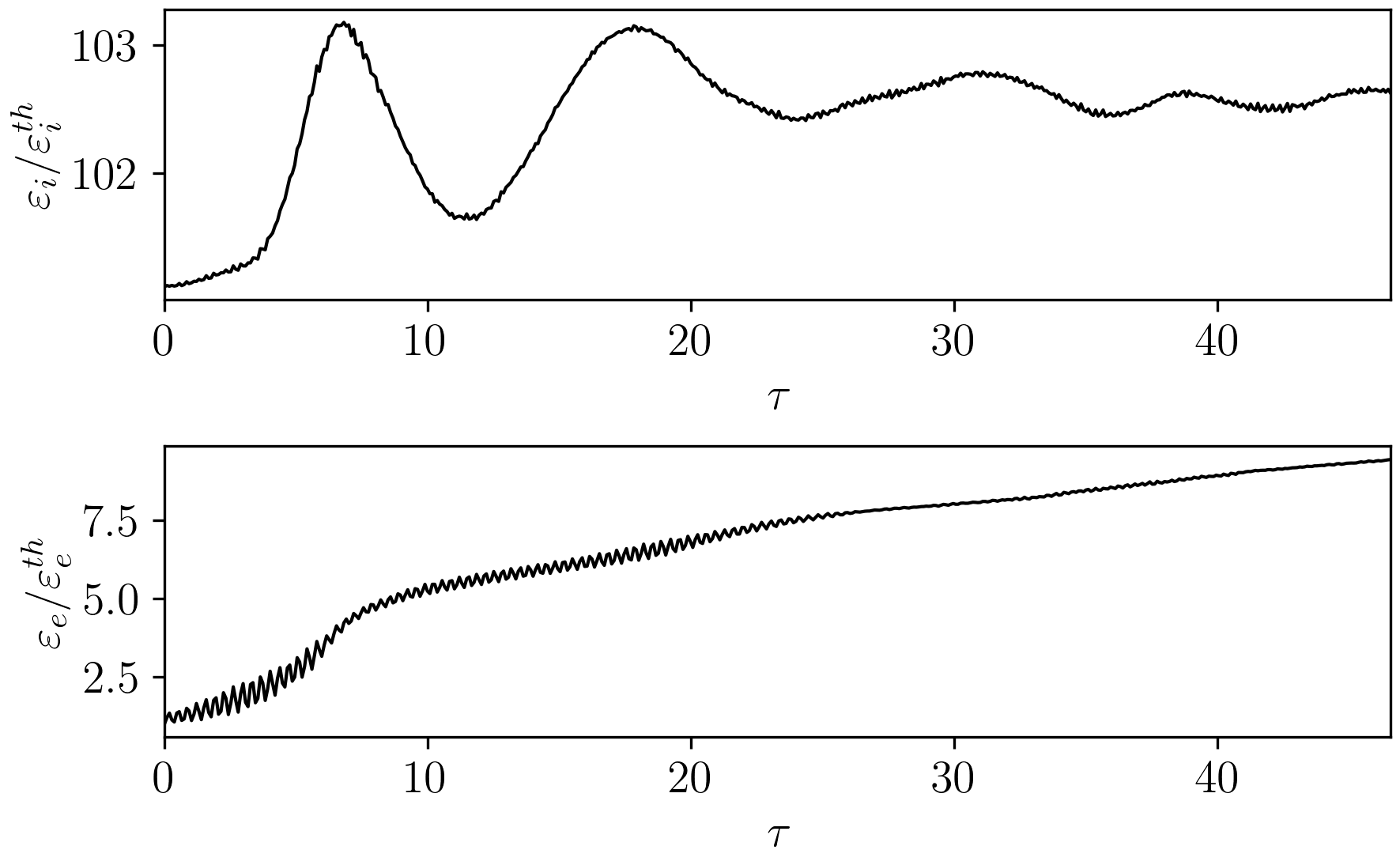
(b)

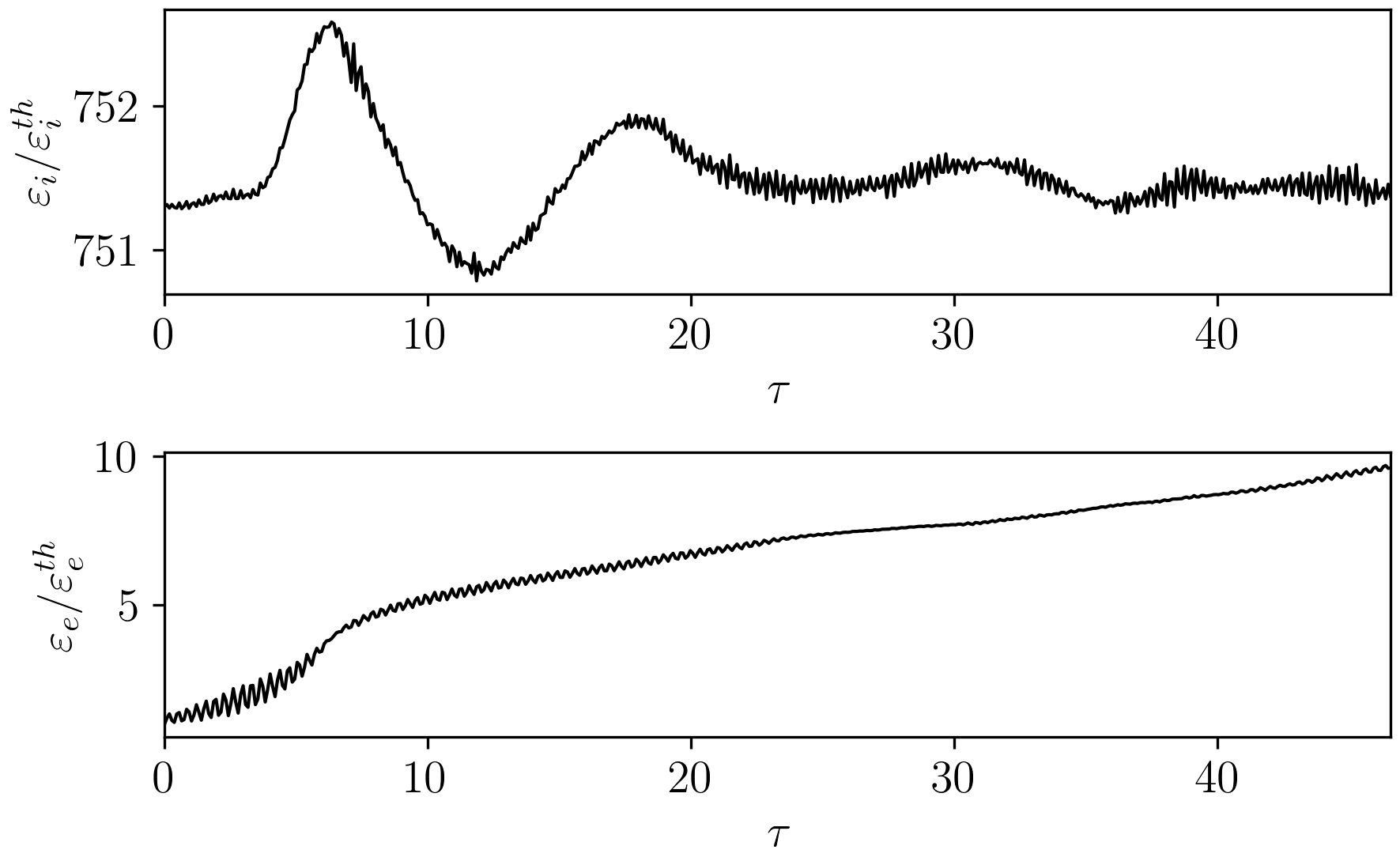
(c)

Figure 8: Evolution of the average kinetic energy of ions (top) and electrons (bottom) for the periodic system with (a) $\tilde{v_{b}}=1.095$, (b) $\tilde{v_{b}}=1.549$, and (c) $\tilde{v_{b}}=4.242$. The average kinetic energy of individual species is normalized by thermal energy of the respective species.

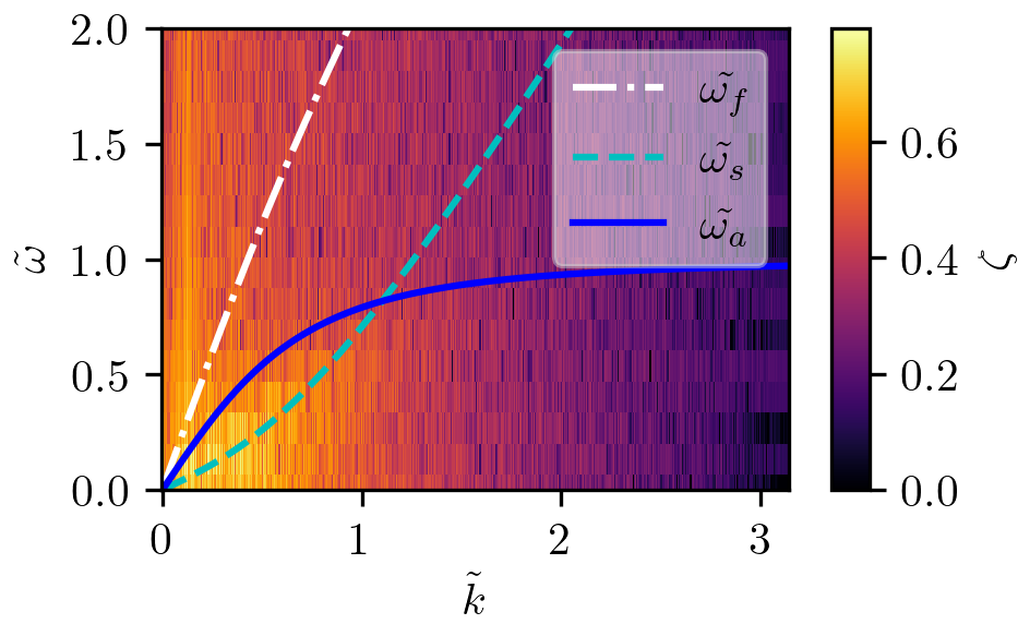
(a)

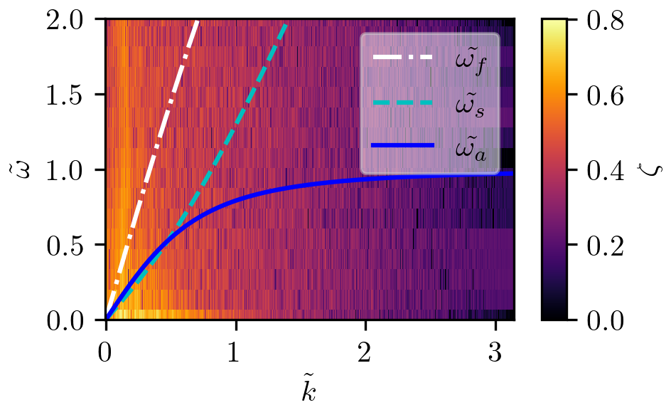
(b)

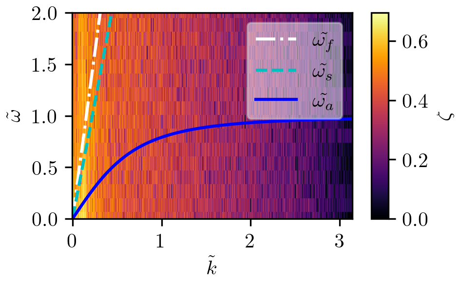
(c)

Figure 9: Plasma dispersion for the periodic system with (a) $\tilde{v_{b}}=1.095$, (b) $\tilde{v_{b}}=1.549$, and (c) $\tilde{v_{b}}=4.242$ along with numerical solutions for eq. 6. The color-map corresponds to the normalized electric field ($\zeta$). The e-field has been normalized with maximum e-field value in each case.

Figure 9 is a representation of collective wave modes in a periodic plasma system excited by ion beams with different velocity. Comparing with our earlier result in fig. 5, one significant observation can be made on the basis of analytic solutions. In fig. 9(a), we can observe the dominant wave mode flips to slow wave mode as we increase the beam velocity from $\tilde{v_{b}}=0.489$) to $\tilde{v_{b}}=1.095$) and the ion acoustic mode is no longer coupled with fast wave mode. As we move towards higher beam velocities ($\tilde{v_{b}}=1.549$, and $\tilde{v_{b}}=4.242$) the two separate branches of beam modes start to merge, which can be confirmed from the subsequent sub-figures in fig. 9. In particular, for the case where the beam velocity is slightly higher than the ion sound speed ($\tilde{v_{b}}=1.549$), the slow beam mode couples with the acoustic branch for low wave numbers. In case of hypersonic beam (fig. 9c), the two wave modes, fast and slow appears to coalesce which is supported by theory as well.

4.2.2 Waves in finite inhomogeneous systems

We will consider the effects of the finite-length system on the evolution of the beam–plasma instability. Since the ion acoustic waves are compressional in nature, the presence of a boundary will lead to significant modification in the plasma properties. To differentiate the effects induced by the boundaries, along with analytic dispersion theory of inhomogeneous medium (section 2.2), we have performed kinetic simulations of the same introducing boundaries and beam as a source at one of the boundaries.

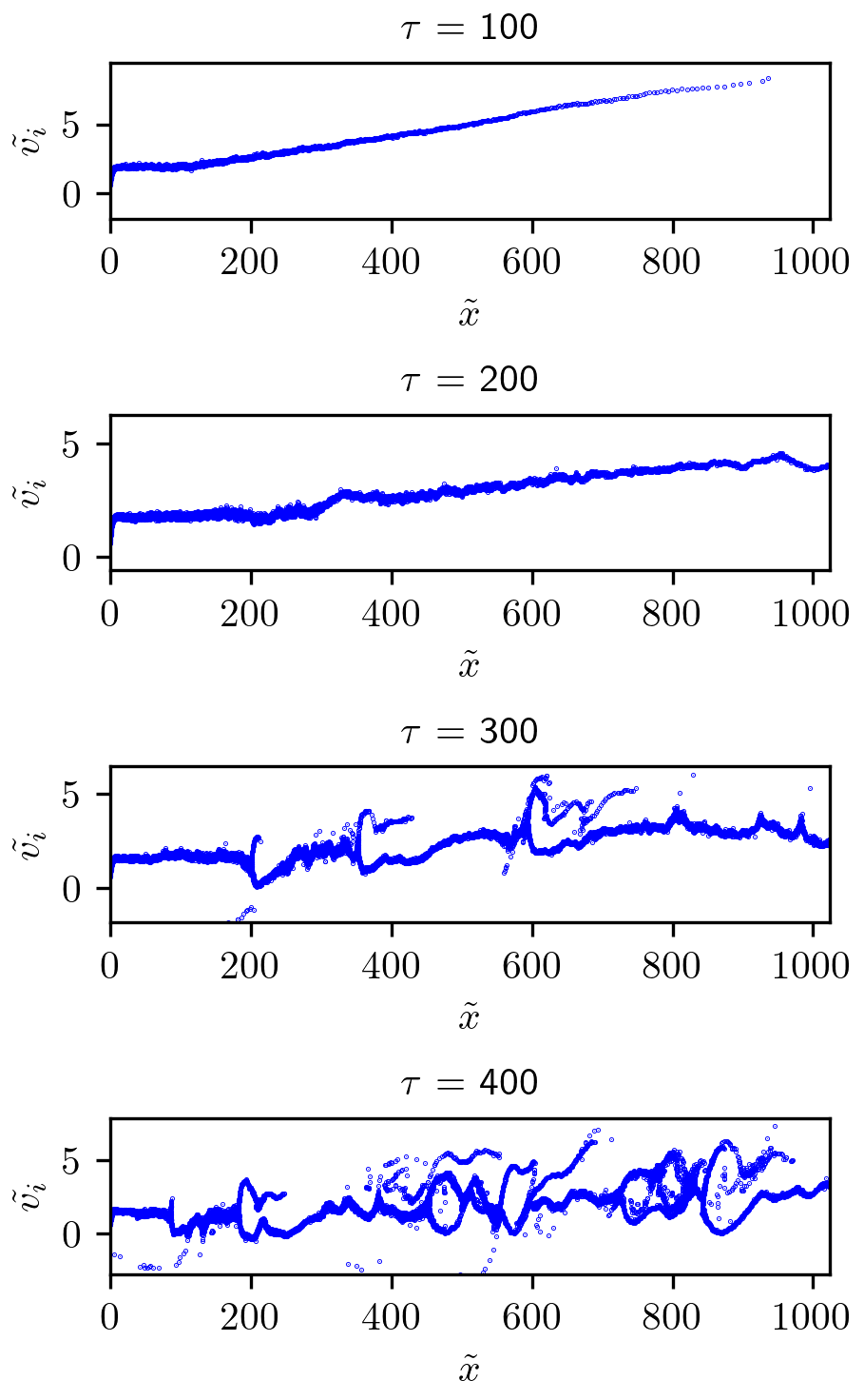
Figure 10: Phase space of ions at different stages of simulation for the bounded system with $\tilde{v_{b}}=0.489$ and $\tilde{x}=1024$. Times are mentioned inside each panel.

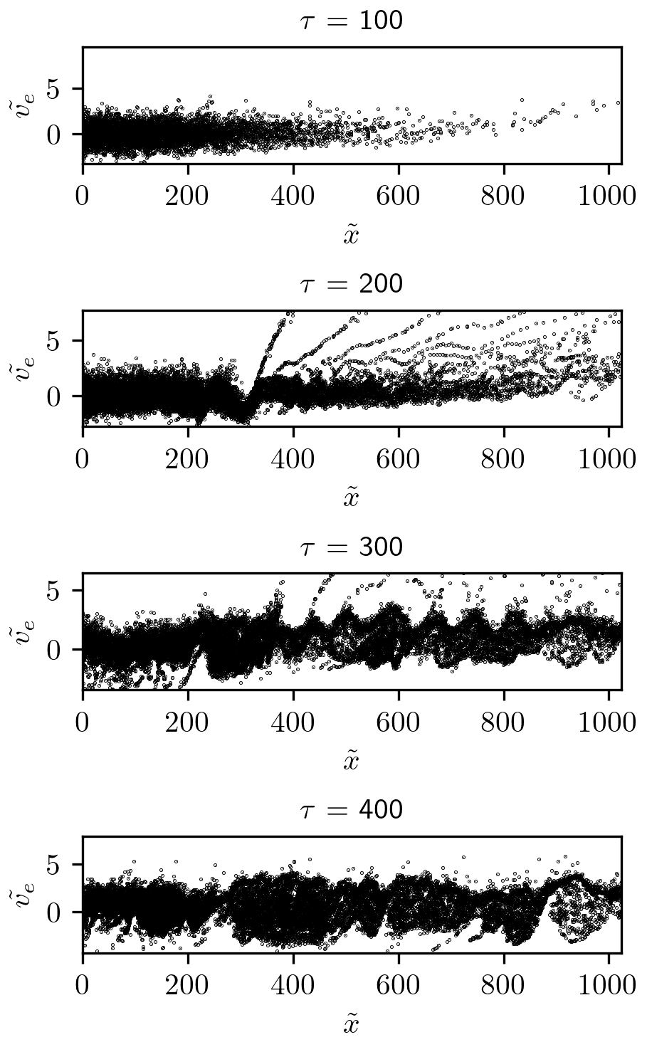
Figure 11: Phase space of electrons at different stages of simulation for the bounded system with $\tilde{v_{b}}=0.489$ and $\tilde{x}=1024$. Times are mentioned inside each panel.

One of the important differences between the periodic and bounded simulations is the total run time. For bounded systems, instead of loading plasma throughout the domain we have injected particles from the left boundary of the domain. The right boundary is assumed to be a perfectly absorbing conductor, i.e. as soon as any particle hits the right boundary it is removed from the domain. For such systems, we run simulation for longer time to reach a sufficiently developed state to study the growth of the irregularities. For all of our cases, we set the limit at $\tau=500$.

Figure 10 and fig. 11 show the phase space structures of individual species over time for system length $\tilde{x}=1024$, whereas fig. 12 and fig. 13 represent the same for system length $\tilde{x}=512$. The visible difference between periodic and bounded system with exactly same plasma parameters comes from the phase spaces of individual species. By point correlation with figure 14, we can see a significant energy growth in the average electron energy at $\tau\sim 100$ and around $\tau\sim 200$. Here, one can make an important observation in terms of the beam acceleration. As soon as the beam enters into the system, it starts to accelerate towards the boundary. After reaching the boundary, the acoustic branch undergoes a reflection and due to coupling between positive and negative energy modes, the acoustic wave mode becomes unstable as suggested by Koshkarov et al. [54].

One of the important mechanisms behind the ion sound instability to occur in bounded systems is charge separation. As we increase the system length, the charge separation becomes less prominent resulting in decreasing instability growth rate [54]. For long systems where $\lambda_{D}\ll L$, the medium is considered weakly dispersive i.e. $k\lambda_{D}\ll 1$. For a fixed-length system, the instability growth rate is a function of the ion beam velocity ($\tilde{v_{b}}$).

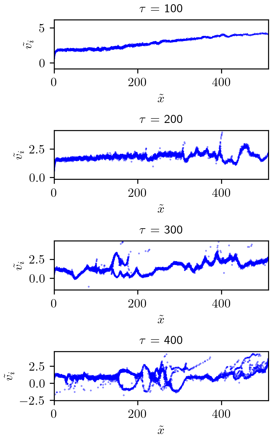
Figure 12: Phase space of ions at different stages of simulation for bounded system with $\tilde{v_{b}}=0.489$ and $\tilde{x}=512$. Times are mentioned inside each panel.

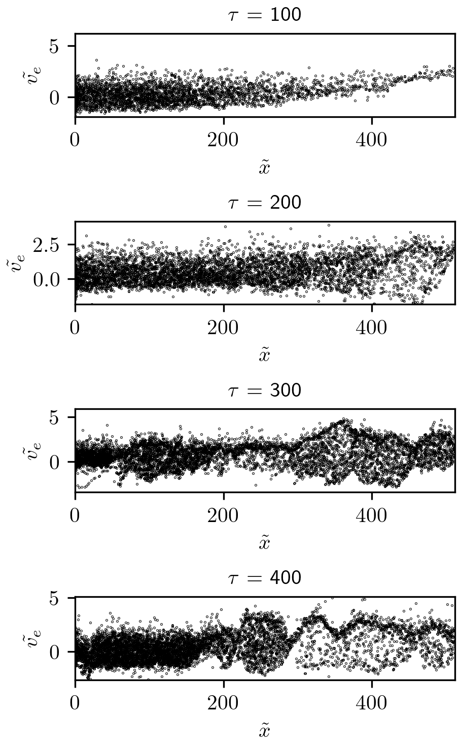
Figure 13: Phase space of electrons at different stages of simulation for bounded system with $\tilde{v_{b}}=0.489$ and $\tilde{x}=512$. Times are mentioned inside each panel.

Figure 12 and fig. 13 show the phase space structure of ions and electrons over time for the system length $\tilde{x}=512$. In comparison with fig. 10 and fig. 11, the dependency of instability growth on boundary is visible: in the former case the phase space holes are more prominent at an earlier stage ($\tau\sim 200$).

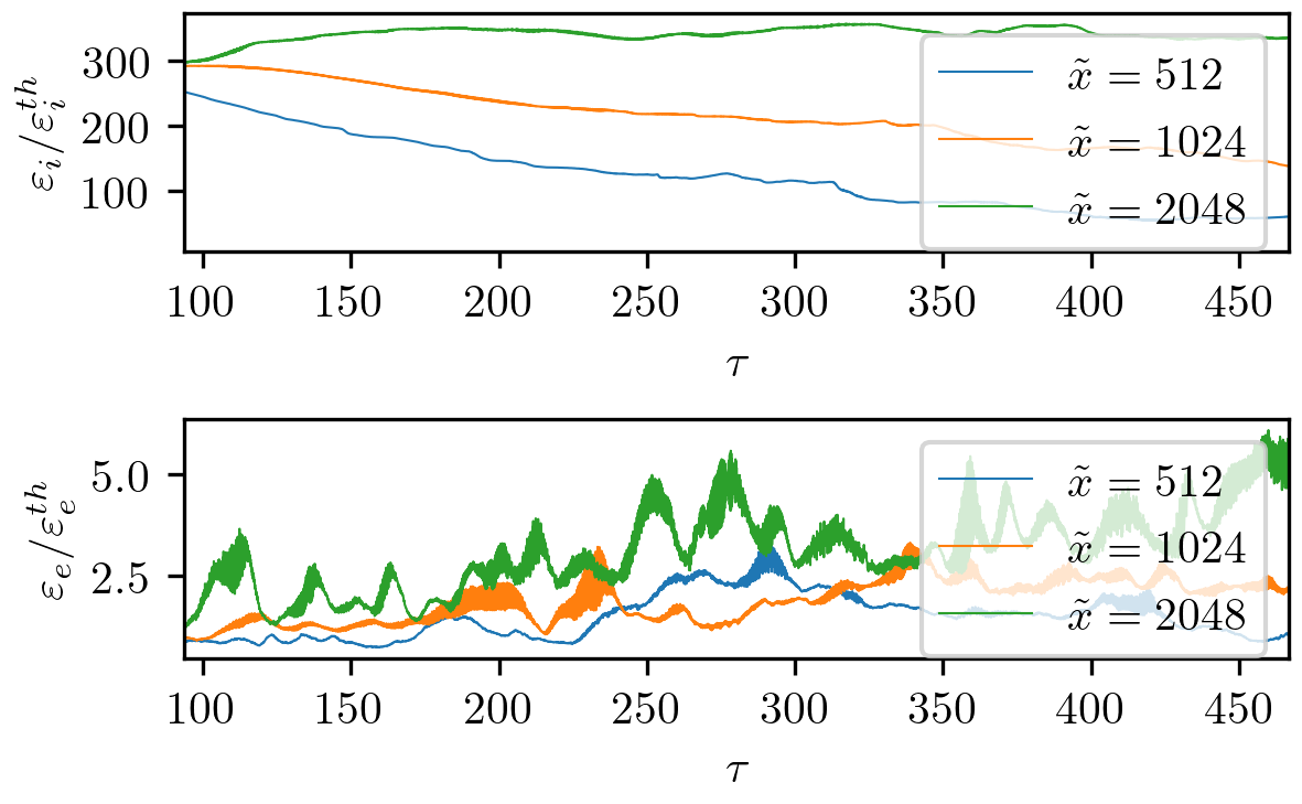
(a)

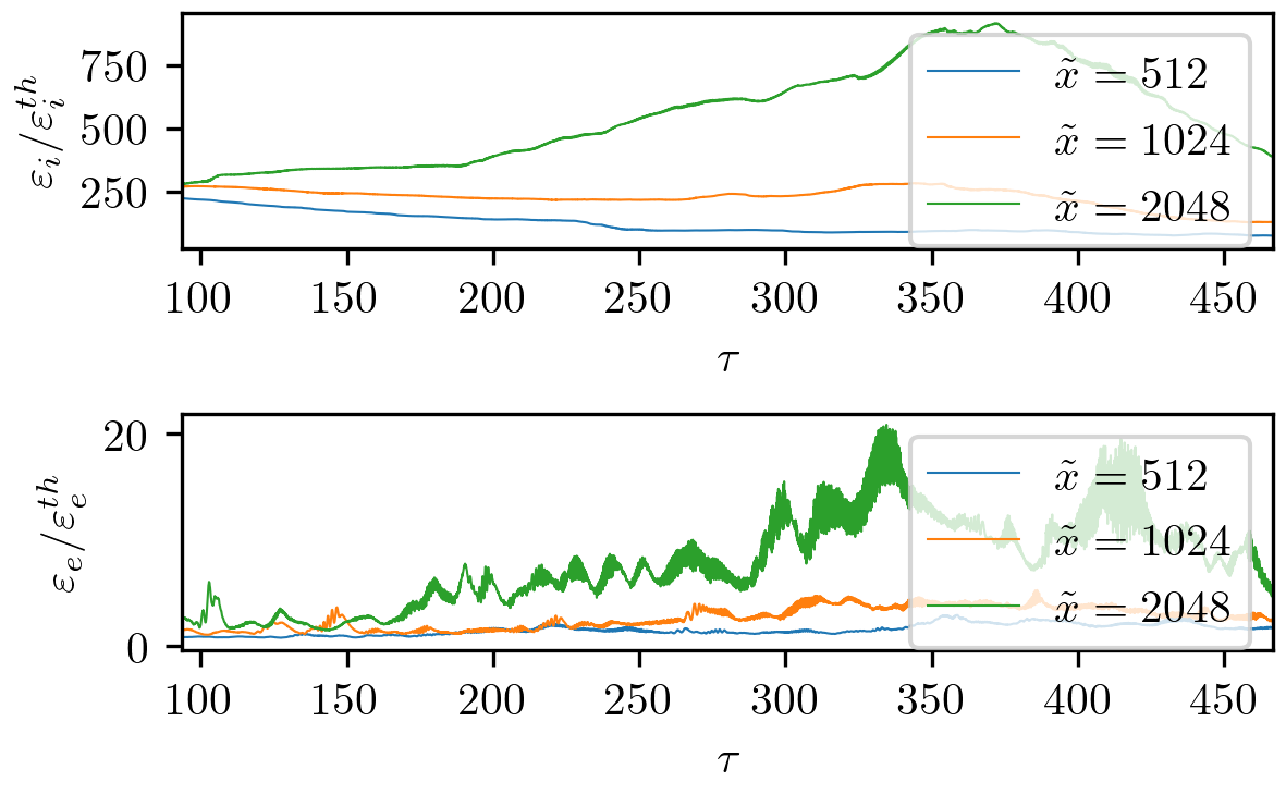
(b)

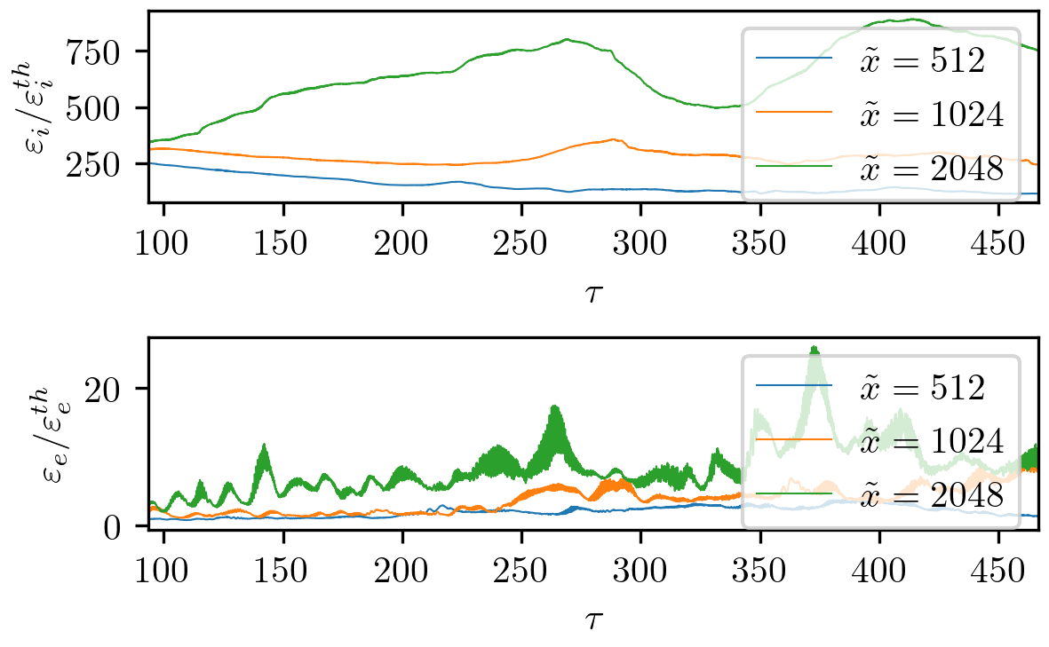
(c)

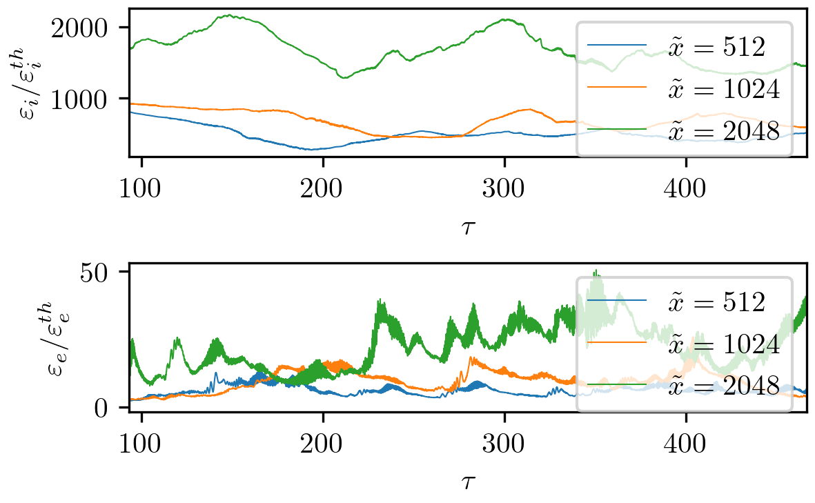
(d)

Figure 14: Evolution of the average kinetic energy of ions (top) and electrons (bottom) for bounded systems with (a) $\tilde{v_{b}}=0.489$, (b) $\tilde{v_{b}}=1.095$, (c)$\tilde{v_{b}}=1.549$, and (d) $\tilde{v_{b}}=4.242$. The average kinetic energy of individual species are normalized by thermal energy of the respective species.

Figure 14 gives us an overview on the evolution of the average kinetic energy of individual species for different system lengths ($\tilde{x}$) and beam velocities ($v_{b}$). For the subsonic case (see fig. 14 (a)) with lengths $\tilde{x}=512$, and $\tilde{x}=1024$, the average kinetic energies for electrons and ions seem to follow the same trend. At around $\tau\sim 100$, as the instability starts to develop in the system ($\tilde{x}=512$), the ion energy falls rapidly and transfers energy to electrons. One important observation for sonic case is the longer system length takes greater time to develop instability. For sonic and supersonic cases (see fig. 14b and fig. 14c) due to the higher beam velocity, the system starts to support the wave growth faster and the energy becomes oscillatory. For near hypersonic case (see figure 14 (d)), we did not notice any difference in the trend. From fig. 14 it is clear that the growth is stronger for systems with longer lengths as compared to shorter ones unlike the case reported by Koshkarov et al. [54]. The difference may have been caused by type of beam source used in the respective systems. The stronger growth for the longer system can be explained in terms of average kinetic energies for particle (see figure 14). For shorter systems, the instability is triggered faster and in due process the ions start to loose their energy to the electrons. Therefore, the wave modes start to disperse faster as compared to the larger systems. Due to the presence of the conducting boundary, the particles are removed as soon as they hit the boundary leading to a self-consistent formation of the sheath. The presence of sheath influences the particle flow to the boundary. Shorter system gets affected strongly in contrast to longer systems. In figures 10 and 12, we can see that for the same $\tilde{v_{b}}$, the ion velocities are limited to $\sim 3$ for shorter system, whereas ions have higher velocities ($\sim 5$) in the larger system.

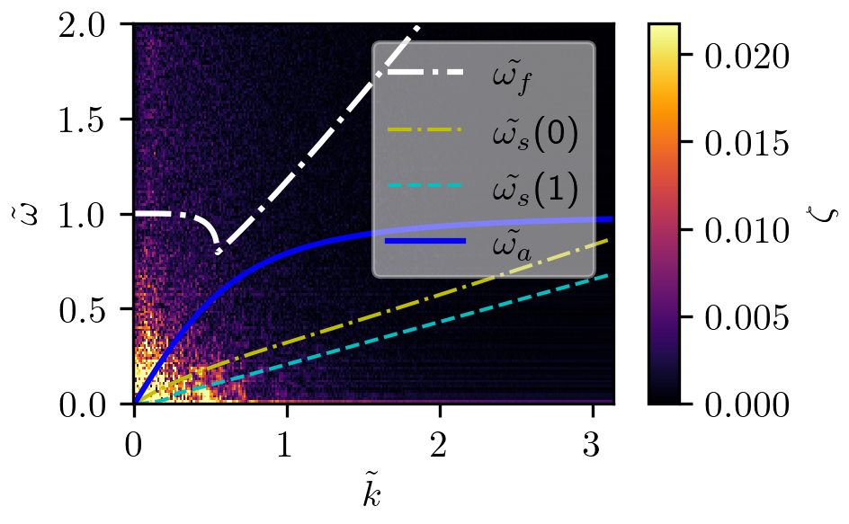
(a)

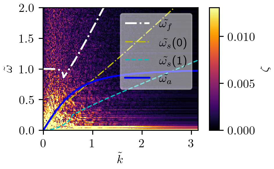
(b)

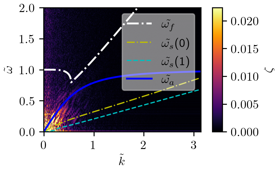
(c)

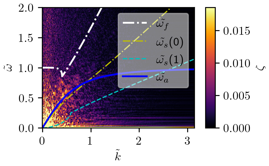
(d)

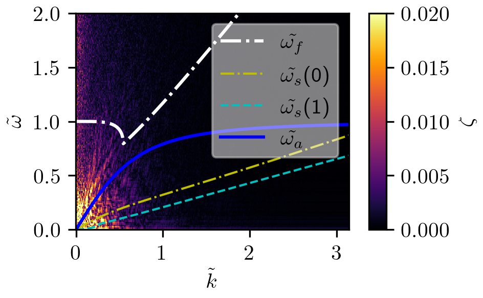
(e)

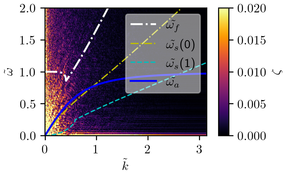
(f)

Figure 15: Plasma dispersion for bounded systems with (a) $\tilde{v_{b}}=0.489$ and $\tilde{x}=512$, (b) $\tilde{v_{b}}=1.095$ and $\tilde{x}=512$, (c) $\tilde{v_{b}}=0.489$ and $\tilde{x}=1024$, (d) $\tilde{v_{b}}=1.095$ and $\tilde{x}=1024$, (e) $\tilde{v_{b}}=0.489$ and $\tilde{x}=2048$, and (f) $\tilde{v_{b}}=1.095$ and $\tilde{x}=2048$ along with numerical solutions for eq. 22 ($\tilde{\xi}=-1.0$, $n=100$). Three different wave modes are denoted as $\tilde{\omega_{f}}$ (fast beam mode), $\tilde{\omega_{s}}$ (slow beam mode), and $\tilde{\omega_{a}}$ (acoustic mode). Acoustic wave mode (solid blue curve) is derived using analytical expression separately for comparison. The color-map corresponds to the normalized electric field ($\zeta$). The e-field has been normalized with the maximum e-field value among all cases.

The plasma dispersion for bounded systems are given in fig. 15 for $\tilde{v_{b}}=0.489$ (subsonic), and $\tilde{v_{b}}=1.095$ (sonic). We have also included the numerical solutions for eq. 22 with $\tilde{\xi}=-1.0$, and $n=100$. The wave modes in the bounded system are expected to be different as compared to the periodic/infinite systems (see fig. 7 and fig. 9)[14]. We have observed that for the ion beam driven ion acoustic instability, the acoustic mode has a constant gradient for low wavenumbers(figure 15) [51]. For shorter system length $\tilde{x}=512$, the growth seems to be localized and strongly coupled between available modes. For $\tilde{x}=1024$, and $\tilde{x}=2048$ some smearing patches are visible along the acoustic branch. The larger system length allows the growth of the wave to extend further into the system as its continues to get fed by the beam energy. It is important to mention that the analytic solutions for the fast and slow beam modes are assumed to be valid at low wavenumbers. With respect to analytical solutions at $\tilde{k}\leq 1$, we believe for subsonic cases, $\tilde{x}=512$ (fig. 15(a)) seems to agree up to a certain extent. For larger system lengths, the analytic solution fails to justify the simulation. However, for supersonic cases (fig. 15 right column), the solution for slow wave modes seems to agree with the simulation outcome. For both subsonic and sonic cases, the bright patches are more confined in lower $\tilde{\omega}$ values as we decrease the system length.

The beam velocities for which the system is expected to show ion acoustic instability is generally found near acoustic region. If the velocity is too low it will undergo Landau damping [75], if too high the beam wave mode might not interact with the acoustic branch at all. However, for bounded finite length systems even for hypersonic beam it might trigger instability due to acoustic reflection [54]. Previous report from Koshkarov et al. [54] suggests that for weakly dispersive case such as ours ($\lambda_{D}\ll L$), the wave growth becomes weaker as the charge separation becomes less prominent. For the present study within the given parameters we have not observed such trend from our simulations. However, we do notice a shift in wave modes towards acoustic branch. Our study also confirms that the beam velocity plays a crucial role in triggering the instability in the system. We have put more focus on providing a collective picture of beam driven acoustic instability in subsonic and supersonic range.

5 Summary and Conclusions

The present work addresses the effects of finite-length systems on beam plasma instability for a cold ion beam streaming with warm electrons. It is demonstrated that the presence of a boundary has a strong impact on wave modes excited in such plasmas. For periodic systems, subsonic and sonic cases seem to agree well with the theoretical estimates. For supersonic and near hypersonic cases, the wave mode coupling is stronger between beam modes. For finite system lengths, the instability growth is found to be a complex quantity and coupled between the effects from kinetic and hydrodynamics properties of plasma.

The phase spaces for ions in bounded systems appear to be extremely different from the periodic cases. One of the important reasons for such nature is thought to be the acoustic reflection at the boundary which can destabilize the sound waves. In cases where such acoustic modes couple with ballistic modes ($\omega=kv_{b}$), the effects seem to be stronger.

Inhomogeneous plasmas are generally considered complex. In the present work, alongside theory we have been able to simulate the effects of boundary on beam plasma instability. The implications of the present work will greatly help in understanding the wave modes in ionospheric plasma simulator devices (e.g. plasma devices at University of Oslo, Norway, and at ESTEC in the Netherlands [76]) or any devices with ion sources (e.g. ion thrusters, hollow cathodes, field effect emitters, plasma contactors, etc.) streaming through thermal neutralizing environment.

One of the critical outcomes of this study is to be able to quantify the beam plasma instability. An extensive parameter scan for such systems allows us to configure the modes and control the plasma for several applications. A follow-up work using experimental methods to verify the simulated results is under development.

DATA AVAILABILITY

The data that support the findings of this study are available from the corresponding author upon reasonable request.

References

References

- [1] Richard J Briggs. Electron-stream interaction with plasmas. MIT, 1964.
- [2] GT Birk, AR Crusius-Wätzel, and H Lesch. Hard radio spectra from reconnection regions in galactic nuclei. The Astrophysical Journal, 559(1):96, 2001.
- [3] Avery E Broderick, Christoph Pfrommer, Ewald Puchwein, and Philip Chang. Implications of plasma beam instabilities for the statistics of the fermi hard gamma-ray blazars and the origin of the extragalactic gamma-ray background. The Astrophysical Journal, 790(2):137, 2014.
- [4] Yu Lyubarsky and JG Kirk. Reconnection in a striped pulsar wind. The Astrophysical Journal, 547(1):437, 2001.
- [5] VL Ginzburg and VV Zhelezniakov. On the possible mechanisms of sporadic solar radio emission (radiation in an isotropic plasma). Soviet Astronomy, 2:653, 1958.
- [6] John G Kirk and O Skjæraasen. Dissipation in poynting-flux-dominated flows: the -problem of the crab pulsar wind. The Astrophysical Journal, 591(1):366, 2003.
- [7] Kurt W Weiler and N Panagia. Are crab-type supernova remnants (plerions) short-lived? Astronomy and Astrophysics, 70:419, 1978.
- [8] Hyesung Kang and TW Jones. Acceleration of cosmic rays at large scale cosmic shocks in the universe. arXiv preprint astro-ph/0211360, 2002.
- [9] Reinhard Schlickeiser. Cosmic ray astrophysics. Springer Science & Business Media, 2013.
- [10] B Grant Logan, FM Bieniosek, CM Celata, J Coleman, W Greenway, E Henestroza, JW Kwan, EP Lee, M Leitner, PK Roy, et al. Recent us advances in ion-beam-driven high energy density physics and heavy ion fusion. Nuclear Instruments and Methods in Physics Research Section A: Accelerators, Spectrometers, Detectors and Associated Equipment, 577(1-2):1–7, 2007.
- [11] RC Davidson, BG Logan, JJ Barnard, FM Bieniosek, RJ Briggs, DA Callahan, M Kireeff Covo, CM Celata, RH Cohen, JE Coleman, et al. Us heavy ion beam research for high energy density physics applications and fusion. In Journal de Physique IV (Proceedings), volume 133, pages 731–741. EDP sciences, 2006.
- [12] Igor D Kaganovich, Edward A Startsev, Adam B Sefkow, and Ronald C Davidson. Charge and current neutralization of an ion-beam pulse propagating in a background plasma along a solenoidal magnetic field. Physical review letters, 99(23):235002, 2007.
- [13] Dale R Welch, David V Rose, Carsten Thoma, Adam B Sefkow, Igor D Kaganovich, Peter A Seidl, S Yu Simon, John J Barnard, and Prabir K Roy. Integrated simulation of an ion-driven warm dense matter experiment. Nuclear Instruments and Methods in Physics Research Section A: Accelerators, Spectrometers, Detectors and Associated Equipment, 577(1-2):231–237, 2007.
- [14] Ronald C Davidson, Mikhail A Dorf, Igor D Kaganovich, Hong Qin, Adam Sefkow, Edward A Startsev, Dale R Welch, David V Rose, and Steven M Lund. Survey of collective instabilities and beam–plasma interactions in intense heavy ion beams. Nuclear Instruments and Methods in Physics Research Section A: Accelerators, Spectrometers, Detectors and Associated Equipment, 606(1-2):11–21, 2009.
- [15] PK Roy, SS Yu, E Henestroza, A Anders, FM Bieniosek, J Coleman, S Eylon, WG Greenway, M Leitner, BG Logan, et al. Drift compression of an intense neutralized ion beam. Physical review letters, 95(23):234801, 2005.
- [16] Irving Langmuir. Scattering of electrons in ionized gases. Physical Review, 26(5):585, 1925.
- [17] JR Pierce. Possible fluctuations in electron streams due to ions. Journal of Applied Physics, 19(3):231–236, 1948.
- [18] Andrew V Haeff. Space-charge wave amplification effects. Physical Review, 74(10):1532, 1948.
- [19] David Bohm and Eugene P Gross. Theory of plasma oscillations. a. origin of medium-like behavior. Physical Review, 75(12):1851, 1949.
- [20] David Bohm and Eugene P Gross. Theory of plasma oscillations. b. excitation and damping of oscillations. Physical Review, 75(12):1864, 1949.
- [21] Ira B Bernstein and SK Trehan. Plasma oscillations (i). Nuclear Fusion, 1(1):3, 1960.
- [22] Thomas Howard Stix. The theory of plasma waves. McGraw-Hill, 1962.
- [23] TE Stringer. Electrostatic instabilities in current-carrying and counterstreaming plasmas. Journal of Nuclear Energy. Part C, Plasma Physics, Accelerators, Thermonuclear Research, 6(3):267, 1964.
- [24] SP Talwar and GR Kalra. Stability of gravitating streams. In Annales d’Astrophysique, volume 29, page 507, 1966.
- [25] Kai Fong Lee. Electromagnetic mode in counterstreaming plasmas in a magnetic field. Physical Review, 181(1):447, 1969.
- [26] SN Kathuria and GL Kalra. Two-stream instability in a collisionless plasma. Astrophysics and Space Science, 24(1):133–143, 1973.
- [27] C Lan, P Dong, and J Li. Excitation of electrostatic solitary waves during neutralization of ion beam pulse by plasma. Plasma Sources Science and Technology, 29(10):105013, 2020.
- [28] Tai-Sen F Wang, Paul J Channell, Robert J Macek, and Ronald C Davidson. Centroid theory of transverse electron-proton two-stream instability in a long proton bunch. Physical Review Special Topics-Accelerators and Beams, 6(1):014204, 2003.
- [29] Ronald C Davidson, Hong Qin, and Tai-Sen F Wang. Vlasov-maxwell description of electron-ion two-stream instability in high-intensity linacs and storage rings. Physics Letters A, 252(5):213–221, 1999.
- [30] Ronald C Davidson, Hong Qin, Peter H Stoltz, and Tai-Sen F Wang. Kinetic description of electron-proton instability in high-intensity proton linacs and storage rings based on the vlasov-maxwell equations. Physical Review Special Topics-Accelerators and Beams, 2(5):054401, 1999.
- [31] Ronald C Davidson and Hong Qin. Effects of axial momentum spread on the electron–ion two-stream instability in high-intensity ion beams. Physics Letters A, 270(3-4):177–185, 2000.
- [32] Hong Qin, Edward A Startsev, and Ronald C Davidson. Nonlinear perturbative particle simulation studies of the electron-proton two-stream instability in high intensity proton beams. Physical Review Special Topics-Accelerators and Beams, 6(1):014401, 2003.
- [33] S Humphries Jr, TR Lockner, JW Poukey, and JP Quintenz. One-dimensional ion-beam neutralization by cold electrons. Physical Review Letters, 46(15):995, 1981.
- [34] RN Sudan. Neutralization of a propagating intense ion beam in vacuum. Applied physics letters, 44(10):957–958, 1984.
- [35] BV Oliver, PF Ottinger, and DV Rose. Evolution of a maxwellian plasma driven by ion-beam-induced ionization of a gas. Physics of Plasmas, 3(9):3267–3278, 1996.
- [36] Dale R Welch, DV Rose, BV Oliver, TC Genoni, RE Clark, CL Olson, and SS Yu. Simulations of intense heavy ion beams propagating through a gaseous fusion target chamber. Physics of Plasmas, 9(5):2344–2353, 2002.
- [37] DV Rose, PF Ottinger, DR Welch, BV Oliver, and CL Olson. Numerical simulations of self-pinched transport of intense ion beams in low-pressure gases. Physics of Plasmas, 6(10):4094–4103, 1999.
- [38] Ronald C Davidson and Qin Hong. Physics of intense charged particle beams in high energy accelerators. World Scientific, 2001.
- [39] Martin Reiser and Patrick O’Shea. Theory and design of charged particle beams, volume 312. Wiley Online Library, 1994.
- [40] JR Pierce. Limiting stable current in electron beams in the presence of ions. Journal of Applied Physics, 15(10):721–726, 1944.
- [41] Ronald C Davidson, Igor Kaganovich, Hong Qin, Edward A Startsev, Dale R Welch, David V Rose, and Han S Uhm. Collective instabilities and beam-plasma interactions in intense heavy ion beams. Physical Review Special Topics-Accelerators and Beams, 7(11):114801, 2004.
- [42] Edward A Startsev and Ronald C Davidson. Dynamic stabilization of the two-stream instability during longitudinal compression of intense charged particle beam propagation through background plasma. Nuclear Instruments and Methods in Physics Research Section A: Accelerators, Spectrometers, Detectors and Associated Equipment, 577(1-2):79–85, 2007.
- [43] DV Rose, TC Genoni, DR Welch, EA Startsev, and RC Davidson. Two-stream instability analysis for propagating charged particle beams with a velocity tilt. Physical Review Special Topics-Accelerators and Beams, 10(3):034203, 2007.
- [44] Masao Sumi. Theory of spatially growing plasma waves. Journal of the Physical Society of Japan, 14(5):653–657, 1959.
- [45] GD Boyd, LM Field, and R Wo Gould. Excitation of plasma oscillations and growing plasma waves. Physical Review, 109(4):1393, 1958.
- [46] Igor D Kaganovich, Gennady Shvets, Edward Startsev, and Ronald C Davidson. Nonlinear charge and current neutralization of an ion beam pulse in a pre-formed plasma. Physics of Plasmas, 8(9):4180–4192, 2001.
- [47] Igor D Kaganovich, Edward A Startsev, and Ronald C Davidson. Nonlinear plasma waves excitation by intense ion beams in background plasma. Physics of Plasmas, 11(7):3546–3552, 2004.
- [48] Chaohui Lan and Igor D Kaganovich. Neutralization of ion beam by electron injection: Accumulation of cold electrons. Physics of Plasmas, 27(4):043108, 2020.
- [49] AA Rukhadze. Electromagnetic waves in interpenetrating plasmas. Soviet Physics-Technical Physics, 6(10):900–+, 1962.
- [50] AB Kitsenko and KN Stepanov. Excitation of magnetoacoustic waves in a rarified plasma by a charged-particle beam. Soviet Physics-Technical Physics, 7(3):215, 1962.
- [51] Christopher Rapson, Olaf Grulke, Konstantin Matyash, and Thomas Klinger. The effect of boundaries on the ion acoustic beam-plasma instability in experiment and simulation. Physics of Plasmas, 21(5):052103, 2014.
- [52] Roald Zinnurovič Sagdeev and Albert A Galeev. Nonlinear plasma theory. npt, 1969.
- [53] F Skiff, G Bachet, and F Doveil. Ion dynamics in nonlinear electrostatic structures. Physics of Plasmas, 8(7):3139–3142, 2001.
- [54] O Koshkarov, AI Smolyakov, ID Kaganovich, and VI Ilgisonis. Ion sound instability driven by the ion flows. Physics of Plasmas, 22(5):052113, 2015.
- [55] A Ya Ender, Heidrun Kolinsky, VI Kuznetsov, and H Schamel. Collective diode dynamics: an analytical approach. Physics Reports, 328(1):1–72, 2000.
- [56] H Schamel and S Bujarbarua. Lagrangian description of ion dynamical effects in plasma diodes. Physics of Fluids B: Plasma Physics, 5(7):2278–2285, 1993.
- [57] James C Johnson, Nicola D’Angelo, and Robert L Merlino. A double layer induced ionisation instability. Journal of Physics D: Applied Physics, 23(6):682, 1990.
- [58] Amy M Keesee, Earl E Scime, Christine Charles, Albert Meige, and Rod Boswell. The ion velocity distribution function in a current-free double layer. Physics of plasmas, 12(9):093502, 2005.
- [59] Rida T Farouki, Manoj Dalvie, and Luca F Pavarino. Boundary-condition refinement of the child–langmuir law for collisionless dc plasma sheaths. Journal of applied physics, 68(12):6106–6116, 1990.
- [60] Mohamad Shalaby, Avery E Broderick, Philip Chang, Christoph Pfrommer, Ewald Puchwein, and Astrid Lamberts. The growth of the longitudinal beam–plasma instability in the presence of an inhomogeneous background. Journal of Plasma Physics, 86(2), 2020.
- [61] Mohamad Shalaby, Avery E Broderick, Philip Chang, Christoph Pfrommer, Astrid Lamberts, and Ewald Puchwein. Growth of beam–plasma instabilities in the presence of background inhomogeneity. The Astrophysical Journal, 859(1):45, 2018.
- [62] Luiz Fernando Ziebell, Peter H Yoon, Joel Pavan, and Rudi Gaelzer. Nonlinear evolution of beam-plasma instability in inhomogeneous medium. The Astrophysical Journal, 727(1):16, 2010.
- [63] AA Vedenov, AV Gordeev, and LI Rudakov. Oscillations and instability of a weakly turbulent plasma. Plasma Physics, 9(6):719, 1967.
- [64] T Takakura and H Shibahashi. Dynamics of a cloud of fast electrons travelling through the plasma. Solar Physics, 46(2):323–346, 1976.
- [65] GR Magelssen and DF Smith. Nonrelativistic electron stream propagation in the solar atmosphere and type iii radio bursts. Solar Physics, 55(1):211–240, 1977.
- [66] Richard Fitzpatrick. Plasma physics: an introduction. Crc Press, 2014.
- [67] William Jones. An introduction to the linear theories and methods of electrostatic waves in plasmas. Springer Science & Business Media, 2012.
- [68] Y Nakamura, H Bailung, and R Ichiki. Effects of a slow ion beam on ion-acoustic waves. Physics of plasmas, 11(8):3795–3800, 2004.
- [69] Izrail Solomonovich Gradshteyn and Iosif Moiseevich Ryzhik. Table of integrals, series, and products. Academic press, 2014.
- [70] Daniel Zwillinger. Handbook of differential equations, volume 1. Gulf Professional Publishing, 1998.
- [71] Edmund Taylor Whittaker and George Neville Watson. A course of modern analysis. Courier Dover Publications, 2020.
- [72] Eric W Weisstein. Parabolic cylinder function. https://mathworld. wolfram. com/, 2002.
- [73] John P Verboncoeur, A Bruce Langdon, and NT Gladd. An object-oriented electromagnetic pic code. Computer Physics Communications, 87(1-2):199–211, 1995.
- [74] A Hasegawa. Electrostatic ion acoustic waves. In Solar-Terrestrial Physics, pages 425–452. Springer, 1983.
- [75] ML Sloan and WE Drummond. Nonlinear landau damping of ion acoustic modes. The Physics of Fluids, 13(10):2554–2562, 1970.
- [76] TA Bekkeng, KS Jacobsen, JK Bekkeng, A Pedersen, T Lindem, JP Lebreton, and JI Moen. Design of a multi-needle langmuir probe system. Measurement science and technology, 21(8):085903, 2010.