Tracing the Mott-Hubbard transition
in one-dimensional Hubbard models without Umklapp scattering

Abstract

We apply the density-matrix renormalization group (DMRG) method to a one-dimensional Hubbard model that lacks Umklapp scattering and thus provides an ideal case to study the Mott-Hubbard transition analytically and numerically. The model has a linear dispersion and displays a metal-to-insulator transition when the Hubbard interaction $U$ equals the band width, $U_{\rm c}=W$, where the single-particle gap opens linearly, $\Delta(U\geq W)=U-W$. The simple nature of the elementary excitations permits to determine numerically with high accuracy the critical interaction strength and the gap function in the thermodynamic limit. The jump discontinuity of the momentum distribution $n_{k}$ at the Fermi wave number $k_{\rm F}=0$ cannot be used to locate accurately $U_{\rm c}$ from finite-size systems. However, the slope of $n_{k}$ at the band edges, $k_{\rm B}=\pm\pi$, reveals the formation of a single-particle bound state which can be used to determine $U_{\rm c}$ reliably from $n_{k}$ using accurate finite-size data.

I Introduction

The Mott-Hubbard metal-to-insulator transition poses one of the fundamental and most intriguing problems in condensed-matter many-particle physics.Mott (1990); Gebhard (1997) When there is on average one electron per lattice site in a single $s$-band, and the electrons are supposed to interact only locally with the Hubbard interaction of strength $U$, there must be a transition from a metallic state at $U=0$ to an insulating state at $U>U_{\rm c}$. In generic situations, the critical interaction strength $U_{\rm c}$ should be of the order of the bandwidth $W$ because the Coulomb interaction competes with the electrons’ kinetic energy. Apparently, the interaction-induced metal-to-insulator transition cannot be attacked using perturbation theory and thus poses a true many-body problem that cannot be solved in general even for simple model Hamiltonians such as the single-band Hubbard model.

Indeed, exact, analytic solutions are scarce and restricted to one spatial dimension where the physics often is special. Indeed, the Bethe Ansatz solution Lieb and Wu (1968) shows that the one-band Hubbard model at half band-filling describes an insulator for all finite interactions. This is the generic situation for one dimensional models when the two Fermi points in momentum space are separated by half a reciprocal lattice vector because Umklapp scattering induces a relevant perturbation at half band-filling for all $U>0$.Giamarchi (2004); Sólyom (2009); Kuramoto (2020)

Since the induced gaps for single-particle excitations of the half-filled ground state are exponentially small for small interactions, it is exceedingly difficult to locate the transition and to calculate the size of the gap in numerical simulations that are necessarily restricted to finite chain lengths.

A way out of this dilemma offer modified one-dimensional models, e.g., those with only one Fermi point, where essentially all electrons move in the same direction. An example for such a model is the $1/r$-Hubbard model where the dispersion is linear over the whole first Brillouin zone.Gebhard and Ruckenstein (1992); Gebhard (1997) The standard Hubbard model and the $1/r$-Hubbard model are limiting cases of the $1/\sinh(\kappa r)$-Hubbard model with electron transfer range $1/\kappa$. This model can be solved exactly with the help of the Asymptotic Bethe Ansatz.Sutherland (1971, 1985) With only one Fermi point present at $\kappa=0$, Umklapp scattering is absent, and the $1/r$-Hubbard model displays the Mott-Hubbard transition at a finite value, $U_{\rm c}=W$. The single-particle gap opens linearly above the transition, $\Delta_{1}(U\geq W)=U-W$.

In contrast to generic Bethe-Ansatz solvable models, the spectrum of the $1/r$-Hubbard model is fairly simple and can be expressed in terms of an effective Hamiltonian for four hard-core bosons that represent the four possible sites occupations (Ashkin-Teller model).Gebhard and Ruckenstein (1992); Gebhard (1997) Consequently, the ground-state energy is a simple sum of ${\cal O}(L)$ terms where $L$ is the number of lattice sites. For this reason, the model also provides a perfect testing ground for the development and test of numerical many-particle techniques such as the density-matrix renormalization group (DMRG) method. However, since the electron transfer amplitudes are long-ranged and complex, standard DMRG codes that are tailored for short-range electron transfers and interactions are insufficient.

In this work, we study the Mott-Hubbard transition when it is not driven by Umklapp scattering processes, and present alternative approaches to locate quantum phase transitions in many-particle systems when conventional extrapolations, e.g., for the gap, lead to inconclusive results. We use DMRG to calculate the ground-state energy and the single-particle and two-particle gaps with high accuracy. Moreover, the DMRG permits the calculation of ground-state properties that cannot be accessed through the spectrum, e.g., the momentum distribution $n_{k}(L;U)$, for finite system sizes and interaction strengths. We monitor the Mott-Hubbard transition from the single-particle gap as a function of system size and interaction strength, and also track the Mott-Hubbard transition from $n_{k}$, in the apparent jump discontinuity $q(L;U)$ at the Fermi wave number and in the slope $s_{-\pi}(L;U)$ of the momentum distribution at the band edge.

The successful analysis of the Mott-Hubbard transition in the $1/r$-Hubbard model paves the way for a DMRG study of the $1/r$-Hubbard model with nearest-neighbor and long-range interactions which may change the nature of the Mott-Hubbard transition. We intend to address this latter issue in a forthcoming publication.

Our present work is organized as follows. In Sect. II we define the model and discuss the ground-state properties of interest, namely, the ground-state energy, the single-particle gap, the two-particle gap, and the momentum distribution. In Sect. III we discuss important aspects of our DMRG algorithm and analyze the finite-size dependence of the ground-state energy and of the gaps. In Sect. IV we present the momentum distribution of the $1/r$-Hubbard model from DMRG calculations with up to $L=128$ sites for various interaction strengths $0\leq U\leq W$, and compare it to perturbative results from weak and strong coupling. In Sect. V we show that the simple spectral structure of the $1/r$-Hubbard model permits to locate with high accuracy the critical interaction and the critical exponent for the single-particle gap. The apparent jump in the momentum distribution does not provide a good estimate for the transition. However, the slope of the momentum distribution at the band edge displays a resonance-shape behavior that indicates the existence of a single-particle bound state at the band edge in the thermodynamic limit when $U=U_{\rm c}$. Short conclusions, Sect. VI, close our presentation. The conventional analysis of the finite-size gap data is deferred to appendix A. In appendix B we motivate the observation of a Fano resonance structure in the slope of the momentum distribution at the band edges as a function of the interaction strength.

II Hubbard model with linear dispersion

II.1 Hamiltonian

We address the $1/r$-Hubbard model Gebhard and Ruckenstein (1992); Gebhard (1997)

$$\hat{H}=\hat{T}+U\hat{D}$$ (1)

on a ring with $L$ sites ($L$: even).

In the $1/r$-Hubbard model, the operator for the kinetic energy $\hat{T}$ is given by

$$\hat{T} = \sum_{\begin{subarray}{c}l,m=1\\ l\neq m;\sigma\end{subarray}}^{L}t(l-m)\hat{c}_{l,\sigma}^{+}\hat{c}_{m,\sigma}^{\vphantom{+}}\;,$$ (2)

$$t(r) = (-{\rm i}t)\frac{(-1)^{r}}{d(r)}\;,$$

$$d(r) = \frac{L}{\pi}\sin\left(\frac{\pi r}{L}\right)\;.$$ (3)

The creation and annihilation operators $\hat{c}_{l,\sigma}^{+}$, $\hat{c}_{l,\sigma}^{\vphantom{+}}$ for an electron with spin $\sigma=\uparrow,\downarrow$ on lattice site $l$ obey the usual anti-commutation relations for fermions.

In eq. (3), $d(l-m)$ is the cord distance between the sites $l$ and $m$ on a ring. In the thermodynamic limit and for $|l-m|\ll L$ fixed, we have $d(l-m)=(l-m)+{\cal O}(1/L^{2})$, and the electron transfer amplitude between two sites decays inversely proportional to their distance (‘$1/r$-Hubbard model’).

Since $L$ is even, we have anti-periodic electron transfer amplitudes because $d(L+r)=-d(r)$. Therefore, we must choose anti-periodic boundary conditions

$$\hat{c}_{L+l,\sigma}=-\hat{c}_{l,\sigma}$$ (4)

for the operators, too. With these boundary conditions, the kinetic energy operator is diagonal in Fourier space,

$$\hat{C}_{k,\sigma}^{+} = \frac{1}{\sqrt{L}}\sum_{l=1}^{L}e^{{\rm i}kl}\hat{c}_{l,\sigma}^{+}\;,$$

$$\hat{c}_{l,\sigma}^{+} = \frac{1}{\sqrt{L}}\sum_{k}e^{-{\rm i}kl}\hat{C}_{k,\sigma}^{+}\;,$$

$$k = \frac{(2m+1)\pi}{L}\;,\;m=-\frac{L}{2},\ldots,\frac{L}{2}-1\;,$$ (5)

so that

$$\hat{T}=\sum_{k,\sigma}\epsilon(k)\hat{C}_{k,\sigma}^{+}\hat{C}_{k,\sigma}^{\vphantom{+}}\;,\quad\epsilon(k)=tk\;.$$ (6)

The dispersion relation of the $1/r$-Hubbard model is linear. We set

$$t=\frac{1}{2\pi}$$ (7)

so that the bandwidth is unity, $W\equiv 1$.

The on-site (Hubbard) interaction Hubbard (1963); Gutzwiller (1963); Kanamori (1963) acts locally between two electrons with opposite spins,

$$\hat{D}=\sum_{l=1}^{L}\hat{n}_{l,\uparrow}\hat{n}_{l,\downarrow}\;,\quad\hat{n}_{l,\sigma}=\hat{c}_{l,\sigma}^{+}\hat{c}_{l,\sigma}^{\vphantom{+}}\;,$$ (8)

where $\hat{n}_{l,\sigma}$ counts the number of electrons with spin $\sigma$ on site $l$.

Under the particle-hole transformation

$$\hat{c}_{l,\sigma}^{\vphantom{+}}\mapsto\hat{c}_{l,\sigma}^{+}\quad,\quad\hat{n}_{l,\sigma}\mapsto 1-\hat{n}_{l,\sigma}\;,$$ (9)

the kinetic energy remains unchanged,

$$\hat{T} \mapsto \sum_{\begin{subarray}{c}l,m=1\\ l\neq m;\sigma\end{subarray}}^{L}t(l-m)\hat{c}_{l,\sigma}^{\vphantom{+}}\hat{c}_{m,\sigma}^{+}$$ (10)

$$= \sum_{\begin{subarray}{c}l,m=1\\ l\neq m;\sigma\end{subarray}}^{L}\left[-t(m-l)\right]\hat{c}_{l,\sigma}^{+}\hat{c}_{m,\sigma}^{\vphantom{+}}=\hat{T}$$

because $t(-r)=-t(r)$.

Furthermore, the operator for the double occupancy transforms as

$$\hat{D}\mapsto\sum_{l=1}^{L}(1-\hat{n}_{l,\uparrow})(1-\hat{n}_{l,\downarrow})=\hat{D}-\hat{N}+L\;.$$ (11)

Therefore, $\hat{H}(N_{\uparrow},N_{\downarrow})$ has the same spectrum as $\hat{H}(L-N_{\uparrow},L-N_{\downarrow})-U(2L-N)+LU$, where $N=N_{\uparrow}+N_{\downarrow}$.

II.2 Ground-state properties

We are interested in the Mott-Hubbard transition. The transition can be inferred from the single-particle and two-particle gaps and from the momentum distribution.

II.2.1 Ground-state energy and single-particle gap

We denote the ground-state energy by

$$E_{0}(N,L;U)=\langle\Psi_{0}|\hat{H}|\Psi_{0}\rangle$$ (12)

for given particle number $N$, system size $L$, and interaction parameters $U$. Here, $|\Psi_{0}\rangle$ is the normalized ground state of the Hamiltonian (1). We are interested in the thermodynamic limit, $N,L\to\infty$ with $n=N/L$ fixed. We denote the ground-state energy per site and its extrapolated value by

$$e_{0}(N,L;U) = \frac{1}{L}E_{0}(N,L;U)\;,$$

$$e_{0}(n;U) = \lim_{L\to\infty}e_{0}(N,L;U)\;,$$ (13)

respectively.

The single-particle gap is defined by

$$\Delta_{1}(L;U)=\mu_{1}^{+}(L;U)-\mu_{1}^{-}(L;U)\;,$$ (14)

where

$$\mu_{1}^{-}(L;U) = E_{0}(L,L;U)-E_{0}(L-1,L;U)\;,$$

$$\mu_{1}^{+}(L;U) = E_{0}(L+1,L;U)-E_{0}(L,L;U)$$ (15)

are the chemical potentials for adding the last particle to half filling and the first particle beyond half filling, respectively. Due to particle-hole symmetry, we have

$$\mu_{1}^{+}(L;U)=U-\mu_{1}^{-}(L;U)$$ (16)

so that

$$\Delta_{1}(L;U)=U-2\mu_{1}^{-}(L;U)$$ (17)

and

$$\Delta_{1}(U)=\lim_{L\to\infty}\Delta_{1}(L;U)$$ (18)

in the thermodynamic limit.

For finite system sizes, the single-particle gap is always finite, $\Delta_{1}(L;U)>0$, due to the discreetness of the kinetic energy spectrum. When extrapolated to the thermodynamic limit, the gap $\Delta_{1}(U)$ vanishes in the metallic phase but remains finite in the insulating phase. The limiting cases are

$$\Delta_{1}(U\ll W) = 0\;,$$

$$\Delta_{1}(U\gg W) = U-W\;.$$ (19)

The latter relation can readily be obtained from strong-coupling perturbation theory.Gebhard (1997) Thus, the single-particle gap permits to locate the critical interaction strength for the Mott-Hubbard transition.

II.2.2 Two-particle gap and effective two-particle repulsion

Analogously, the two-particle gap is defined by

$$\Delta_{2}(L;U)=\mu_{2}^{+}(L;U)-\mu_{2}^{-}(L;U)\;,$$ (20)

where

$$\mu_{2}^{-}(L;U) = E_{0}(L,L;U)-E_{0}(L-2,L;U)\;,$$

$$\mu_{2}^{+}(L;U) = E_{0}(L+2,L;U)-E_{0}(L,L;U)$$ (21)

are the chemical potentials for adding the last two particles to half filling and the first two particles beyond half filling, respectively. We always consider the spin symmetry $S=S^{z}=0$. Due to particle-hole symmetry, we have

$$\mu_{2}^{+}(L;U)=2U-\mu_{2}^{-}(L;U)$$ (22)

so that

$$\Delta_{2}(L;U)=2U-2\mu_{2}^{-}(L;U)$$ (23)

and

$$\Delta_{2}(U)=\lim_{L\to\infty}\Delta_{2}(L;U)$$ (24)

in the thermodynamic limit.

The two added particles repel each other so that, in the thermodynamic limit, they are infinitely separated from each other. Therefore, we will have

$$\Delta_{2}(U)=2\Delta_{1}(U)\;.$$ (25)

For finite systems, we expect the interaction energy

$$e_{\rm R}(L;U)=\Delta_{2}(L;U)-2\Delta_{1}(L;U)={\cal O}(1/L)>0$$ (26)

to be positive, of the order $1/L$.

II.2.3 Momentum distribution

We also study the spin-summed momentum distribution in the ground state at half band-filling, $N=L$,

$$n_{k}(L;U)=\langle\Psi_{0}|\hat{n}_{k,\uparrow}+\hat{n}_{k,\downarrow}|\Psi_{0}\rangle$$ (27)

with $\hat{n}_{k,\sigma}=\hat{C}_{k,\sigma}^{+}\hat{C}_{k,\sigma}^{\vphantom{+}}$. In the metallic phase, the $1/r$-Hubbard model can be classified as a pure $g_{4}$-model within the $g$-ology scheme.Mahan (2007); Giamarchi (2004); Sólyom (2009); Kuramoto (2020) For this reason, it displays a jump discontinuity at the Fermi energy $E_{\rm F}=0$ with wave vector $k_{\rm F}=0$ (‘non-interacting’, or ‘free’, Luttinger liquidKuramoto and Yokoyama (1991)) in contrast to regular Luttinger liquids that display algebraic singularities at $k_{\rm F}$.Schönhammer and Meden (1993); Voit (1993); Giamarchi (2004)

In the insulating phase, $n_{k}(U)$ is a continuous function of $k$ within the first Brillouin zone, $-\pi<k<\pi$. The limiting cases thus are

$$n_{k}(L;U=0)=\begin{cases}\begin{array}[]{@{}lll@{}}2&\text{for}&-\pi<k<0\\ 0&\text{for}&0<k<\pi\end{array}\end{cases}$$ (28)

and $n_{k}(L;U\to\infty)=1$. The jump discontinuity in $n_{k}(U)=\lim_{L\to\infty}n_{k}(L;U)$ at the Fermi energy vanishes at the Mott-Hubbard transition. The discontinuity may thus be used to located the critical interaction strength.

III Ground-state energy and gaps

In this section we compile some analytic results for the $1/r$-Hubbard model whose spectrum was conjectured to be identical to that of an effective Hamiltonian for hard-core bosons.Gebhard and Ruckenstein (1992); Gebhard (1997) Therefore, the exact ground-state energy, the single-particle gap, and the two-particle gap are known for all system sizes $L$.

These analytic results are accurately reproduced by DMRG for up to $L=128$ lattice sites. This confirms the validity of the conjectured effective Hamiltonian.Gebhard and Ruckenstein (1992); Gebhard (1997) Moreover, it demonstrates the efficiency of the employed DMRG code for complex-valued, long-range electron transfer amplitudes.

III.1 DMRG method

We apply the real-space DMRG algorithm White (1992, 1993); Schollwöck (2005) to the Hamiltonian (1). Complex-valued and long-range electron transfer amplitudes and anti-periodic boundary conditions require an elaborate DMRG code that was originally designed for calculations in quantum chemistry utilizing various optimization protocols based on quantum information theory.Szalay et al. (2015)

The model has a gapless energy spectrum up to a critical Coulomb coupling. Therefore, a thorough control of the numerical accuracy is crucial to obtain accurate values for the gap and for static single-particle correlation functions. We make use of the SU(2) spin symmetry McCulloch (2007); Tóth et al. (2008) and of the dynamic block-state selection approach (DBSS),Legeza et al. (2003); Legeza and Sólyom (2004) where the a-priori value for the truncation errors was set to $\delta\varepsilon_{\rm Tr}=10^{-6}$ for $L\leq 128$. The maximal number of selected SU(2) multiplets according to this accuracy demand turns out to be around $M_{\rm SU(2)}=4000\ldots 5000$, corresponding to about $M_{\rm U(1)}>10000$ DMRG block states when only the total spin in $z$-direction is taken into account. We use between seven and eleven DMRG sweeps.

When we compare our DMRG data with the exact results for the ground-state energies at finite system size $L\leq 128$ and interaction strength $U\leq 2W$, we obtain an absolute error of $\Delta E_{0}(N,L;U)=E_{0}^{\rm DRMG}(N,L;U)-E_{0}(N,L;U)\lesssim 10^{-4}$ in the energy of the ground state at half band-filling, $N=L$, and with one or two extra particles (or holes) in the half-filled ground state, $N=L\pm 1$ and $N=L\pm 2$, respectively. We used both Davidson and Lánczos algorithms as subroutines for the matrix diagonalization. We found the Lánczos algorithm to be more stable in all DMRG runs. As tests for the SU(2) and U(1) algorithms we numerically reproduced the analytic data for the ground-state energy at half band-filling with at least six digits accuracy for $U=0.5$, $U=1$, and $U=2$.

We determine the momentum distribution from the Fourier transformation of the single-particle density matrix in position space,

$$n_{k,\sigma}=\frac{1}{L}\sum_{i,j}e^{{\rm i}k(i-j)}\langle\Psi_{0}|\hat{c}_{i,\sigma}^{+}\hat{c}_{j,\sigma}^{\vphantom{+}}|\Psi_{0}\rangle\;.$$ (29)

The finite-size scaling analysis is carried out for system sizes up to $L=128$ lattice sites. Note that enforced the anti-periodic boundary conditions lead to a faster convergence of the ground-state expectation values as a function of inverse system size than in the case of open boundary conditions. Roughly speaking, the system size must be a factor of two larger for open boundary conditions than for (anti-)periodic boundary conditions to obtain the same magnitude for the finite-size corrections.

III.2 Ground-state energy

For all system sizes and particle numbers, the spectrum of the $1/r$-Hubbard model with on-site interactions and anti-periodic boundary conditions can be obtained from the hard-core boson Hamiltonian Gebhard and Ruckenstein (1992)

$${\cal H} = \sum_{K}h_{K,\uparrow}^{s}n_{K,\uparrow}^{s}+h_{K,\downarrow}^{s}n_{K,\downarrow}^{s}+h_{K}^{d}n_{K}^{d}+h_{K}^{e}n_{K}^{e}$$ (30)

$$+\sum_{K}J_{K}\left[n_{K-\Delta}^{d}n_{K}^{e}-n_{K-\Delta,\uparrow}^{s}n_{K,\downarrow}^{s}\right]\;,$$

$$h_{K,\sigma} = \frac{tK}{2}\;,$$

$$h_{K}^{e} = -\frac{tK}{2}\;,$$

$$h_{K}^{d} = U-\frac{tK}{2}\;,$$

$$J_{K} = \frac{t(2K-\Delta)-U+\sqrt{W^{2}+U^{2}-2tU(2K-\Delta)}}{2}\;.$$

In eq. (30) we have

$$K=\frac{\pi}{L}\left(2m_{K}+1\right)\;,\;m_{K}=-\frac{L}{2},\ldots,\frac{L}{2}-1\;,\;\Delta=\frac{2\pi}{L}\;.$$ (31)

Note that every ‘site’ $K$ is occupied with either of the four bosons $\{\uparrow,\downarrow,e\equiv\circ,d\equiv\uparrow\downarrow\}$.

In the boson language, the ground state is represented by

$$|\Psi_{0}\rangle=|\framebox{$\uparrow,\downarrow$},\framebox{$\uparrow,\downarrow$},\ldots\framebox{$\uparrow,\downarrow$},\circ,\circ,\ldots\circ\rangle$$ (32)

when $N$ is even. The first spin is at $K=-\pi+\pi/L$, the last spin is at

$$K_{\rm F}=\frac{\pi}{L}\left(N-\frac{L}{2}-1\right)\;.$$ (33)

The ground-state energy is thus given by

$$E_{0}(N,L;U)=\sum_{K\leq K_{\rm F}}tK-\sum_{l=1}^{N/2}J_{K=-\pi+3\pi/L+2\Delta(l-1)}$$ (34)

where we use that $\sum_{K}K=0$. The expression for the ground-state energy per site can be simplified to

$$e_{0} = \frac{1}{4}n(n-1)+\frac{U}{4}n$$

$$-\frac{1}{2L}\sum_{r=0}^{(N/2)-1}\sqrt{1+U^{2}-4U(2r+1-L/2)/L}$$

with $n=N/L$ and $e_{0}\equiv e_{0}(N,L;U)$.

In the thermodynamic limit, we find

$$e_{0}(n;U) = \frac{1}{4}n(n-1)+\frac{U}{4}n$$

$$-\frac{1}{24U}\left[(1+U)^{3}-\left((1+U)^{2}-4Un\right)^{3/2}\right]$$

for the ground-state energy per site for $n=N/L\leq 1$, with corrections of the order $1/L^{2}$ for $U\neq W=1$. At the Mott transition point, $U=W$, the finite-size corrections are of the order $1/L^{3/2}$.

Table 1 gives the ground-state energy for various system sizes and values $U=W/2,W,2W$. The DMRG reproduces the values with an accuracy of at least six digits. On the one hand, this confirms the validity of the effective hard-core boson model for system sizes up to $L=128$. On the other hand, it demonstrates the accuracy and efficiency of the DMRG code for Hubbard models with complex-valued long-range electron transfers.

$L$	$-e_{0}(0.5)$	$-e_{0}(1)$	$-e_{0}(2)$
4$A^{A}$	$0.148612632415$	$0.0915063509461$	$0.0472252648292$
6	$0.147186159589$	$0.0880376668043$	$0.0443723191770$
8	$0.146629075934$	$0.0864886985031$	$0.0432581518589$
16	$0.146044361095$	$0.0845160860650$	$0.0420887221900$
32	$0.145887166056$	$0.0837683378403$	$0.0417743321119$
64	$0.145846869387$	$0.0834913432390$	$0.0416937387731$
128	$0.145836722450$	$0.0833902516076$	$0.0416734449005$
$\infty$	$0.145833333333$	$0.0833333333333$	$0.0416666666667$

Table 1: Ground-state energy per site $e_{0}(L,L;U)$ of the $1/r$-Hubbard model with anti-periodic boundary conditions for various values of $U$ and $N=L=4,6,8,16,32,64,128$ (half band filling). The DMRG reproduces the data with an accuracy of at least six digits.

III.3 Single-particle gap

For the calculation of $E_{0}(L-1,L;U)$ we need the ground state for an odd number of particles, say with $S^{z}=1/2$. In the bosonic representation it is given by

$$|\Psi_{0}\rangle=|\uparrow,\framebox{$\uparrow,\downarrow$},\framebox{$\uparrow,\downarrow$},\ldots\framebox{$\uparrow,\downarrow$},\circ\rangle\;.$$ (37)

It has the energy

$$E_{0}(L-1,L;U)=-tK_{m}-\sum_{l=1}^{L/2-1}J_{K=-\pi+3\pi/L+\Delta+2\Delta(l-1)}\;,$$ (38)

where we used that $\sum_{K}K=0$ and $K_{m}=\pi-\pi/L$.

This can be simplified to

$$E_{0}^{-} = \frac{UL}{4}-\frac{U+1}{2}+\frac{1}{2L}$$

$$-\frac{1}{2}\sum_{r=0}^{(L/2)-2}\sqrt{1+U^{2}-4U(2r+2-L/2)/L}\;,$$

where we used the abbreviation $E_{0}^{-}\equiv E_{0}(L-1,L;U)$. The single-particle gap becomes

$$\Delta_{1}(L;U) = -1+\frac{1}{L}$$

$$-\sum_{r=0}^{(L/2)-2}\sqrt{1+U^{2}-4U(2r+2-L/2)/L}$$

$$+\sum_{r=0}^{(L/2)-1}\sqrt{1+U^{2}-4U(2r+1-L/2)/L}\;.$$

In the thermodynamic limit, we may use the Euler-MacLaurin sum formula for the sums in eq. (III.3) to find ($W\equiv 1$ is the bandwidth)

$$\Delta_{1}(U) = \frac{U-W}{2}+\frac{|U-W|}{2}$$ (43)

$$= \left\{\begin{array}[]{@{}lll@{}}0&\hbox{for}&U\leq U_{\rm c}=W\\[6.0pt] U-W&\hbox{for}&U\geq U_{\rm c}=W\end{array}\right.$$

in the thermodynamic limit. The gap opens linearly at $U_{\rm c}=W$. The same result can also be obtained from the very definition of $\mu_{1}^{-}$. We use eq. (LABEL:eq:ezeroTDL) for the ground-state energy for $n=N/L\leq 1$ and find

$$\mu_{1}^{-}=\left.\frac{\partial e_{0}(n;U)}{\partial n}\right|_{n=1}=\frac{W+U}{4}-\frac{|U-W|}{4}$$ (44)

which also leads to equation (43) for the single-particle gap when we use eq. (17).

$L$	$\Delta_{1}(0.5)$	$\Delta_{1}(1)$	$\Delta_{1}(2)$
4$A^{A}$	0.320867070567	0.567837245196	1.39173414113
6	0.217167734761	0.435424968083	1.26766880285
8	0.164130166884	0.362554806107	1.20326033377
16	0.082919292022	0.236931208089	1.10333858404
32	0.041608809524	0.157825321710	1.05196761904
64	0.020825835837	0.106745012744	1.02602667167
128	0.010415720145	0.073053055090	1.01301894029
$\infty$	0	0	1

Table 2: Single-particle gap $\Delta_{1}(U)$ of the $1/r$-Hubbard model with anti-periodic boundary conditions for $U/W=0.5,1,2$ and system sizes $L=4,6,8,16,32,64,128$ at half band-filling. The DMRG reproduces the data with an accuracy of at least six digits.

Table 2 gives the single-particle gap for various system sizes and values $U=W/2,W,2W$. The DMRG reproduces the values with an accuracy of at least six digits. Again, these results mutually confirm the validity of the analytic formulae and of the DMRG results.

For $U\neq W$, the single-particle gap extrapolates to its value in the thermodynamic limit with corrections of the order $1/L$. At the Mott transition point, $U=W=1$, the finite-size corrections are of the order $1/\sqrt{L}$.

III.4 Two-particle gap

$L$	$\Delta_{2}(0.5)$	$\Delta_{2}(1)$	$\Delta_{2}(2)$
4$A^{A}$	0.866025403784	1.50000000000	3.23205080757
6	0.597095949159	1.14982991426	2.86085856499
8	0.457106781187	0.957106781187	2.66421356237
16	0.237372435696	0.625000000000	2.34974487139
32	0.121516994375	0.416053390593	2.18053398875
64	0.061580085890	0.281250000000	2.09191017178
128	0.031013203202	0.192401695297	2.04640140640
$\infty$	0	0	2

Table 3: Two-particle gap $\Delta_{2}(U/W)\equiv\Delta_{2}(W,U,L)/W$ of the $1/r$-Hubbard model with anti-periodic boundary conditions for $U/W=0.5,1,2$ and $L=4,6,8,16,32,64,128$ at half band-filling. The DMRG reproduces the data with an accuracy of at least six digits.

For the calculation of the two-particle gap, we again use the energy formula (34). We thus find

$$\mu_{2}^{-}=\frac{U+W}{2}-\frac{W}{L}-\frac{1}{2}\sqrt{(W-U)^{2}+4WU/L}\;.$$ (45)

because only the energy difference of the last two sites remains in the difference in the ground-state energies for $N=L$ and $N=L-2$ particles on $L$ sites. Thus, from eq. (23) we find

$$\Delta_{2}(L;U)=U-W+\frac{2W}{L}+\sqrt{(W-U)^{2}+\frac{4WU}{L}}\;,$$ (46)

which reduces to

$$\Delta_{2}(U)=U-W+|W-U|=2\Delta_{1}(U)$$ (47)

in the thermodynamic limit, as expected. Some values for finite system sizes are collected in table 3. The DMRG reproduces the values with an accuracy of at least six digits. Again, these results mutually confirm the validity of the analytic formulae and of the DMRG results.

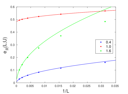
Figure 1: Effective repulsive energy $e_{\rm R}(L;U)$ of two holes in the half-filled ground state, eq. (26), multiplied by $\sqrt{L}$ as a function of inverse system size ($L=32,64,128,256,512,1024$) for the $1/r$-Hubbard model for $U=0.4$, $U=U_{\rm c}=1$, and $U=1.6$. The lines result from eq. (48) for $U=0.4$ and $U=1.6$, and from eq. (49) for $U=1$.

In Fig. 1 we show the effective repulsive energy of the two holes confined to $L$ sites, eq. (26). Away from the transition, $e_{\rm R}(L;U)\sim 1/L$ which is characteristic for a two-particle repulsion of finite range,

$$e_{\rm R}(L;U<U_{\rm c}) \approx \frac{2U}{1-U^{2}}\frac{1}{L}\;,$$

$$e_{\rm R}(L;U>U_{\rm c}) \approx \frac{2U^{2}}{U^{2}-1}\frac{1}{L}\;.$$ (48)

It is only at the critical interaction, $U_{\rm c}=1$, that the correlation length diverges which results in $e_{\rm R}(L;U_{\rm c}=1)\sim 1/\sqrt{L}$. For this reason, we actually plot $\sqrt{L}e_{\rm R}(L;U)$ in Fig. 1 which extrapolates to a finite value in the thermodynamic limit when $U=U_{\rm c}=1$,

$$\sqrt{L}e_{\rm R}(L;U=U_{\rm c})\approx\left(2+4(2\sqrt{2}-1)\zeta(-1/2)\right)+\frac{1}{2\sqrt{L}}\;.$$ (49)

In the derivation of eqs. (48) and (49), we used Mathematica Wolfram Research, Inc. (2021) to perform the sums and the expansion in $1/L$. Numerically, $\left(2+4(2\sqrt{2}-1)\zeta(-1/2)\right)\approx 0.479581$.

IV Momentum distribution

The momentum distribution cannot be calculated analytically in general but can only be evaluated perturbatively for small coupling to order $(U/W)^{2}$ and for strong coupling to order $W/U$. DMRG, however, provides $n_{k}$ for systems with up to 128 sites for all interaction strengths.

IV.1 Momentum distribution at weak coupling

IV.1.1 Wave function in weak coupling

As shown by Girndt and one of us,Gebhard and Girndt (1994) see also Dzierzawa et al.,Dzierzawa et al. (1995) the Gutzwiller wave function Gutzwiller (1963)

$$|\Psi_{\rm G}(g)\rangle=g^{\hat{D}}|{\rm FS}\rangle$$ (50)

reproduces the ground-state energy of the $1/r$-Hubbard model (1) at half band-filling to order $U^{2}$. Here, $|{\rm FS}\rangle$ is the paramagnetic Fermi-sea ground state at $U=0$ and $g$ is a variational parameter with $1\geq g>0$ for $0\leq U<\infty$. By construction, the variational state is exact for $U=0$ where $g=1$.

At half band-filling we have Metzner and Vollhardt (1987)

$$\bar{d}(g) = \frac{1}{L}\frac{\langle\Psi_{\rm G}(g)|\hat{D}|\Psi_{\rm G}(g)\rangle}{\langle\Psi_{\rm G}(g)|\Psi_{\rm G}(g)\rangle}$$ (51)

$$= \frac{g^{2}}{2(1-g^{2})^{2}}\left[-(1-g^{2})-\ln(g^{2})\right]$$

for the average double occupancy and

$$\bar{T}(g) = \frac{1}{L}\frac{\langle\Psi_{\rm G}(g)|\hat{T}|\Psi_{\rm G}(g)\rangle}{\langle\Psi_{\rm G}(g)|\Psi_{\rm G}(g)\rangle}$$ (52)

$$= -\frac{1}{4}-\left(\frac{g-1}{g+1}\right)\left(\frac{1}{4}-\bar{d}(g)\right)$$

for the average kinetic energy (bandwidth $W=2\pi t\equiv 1$). For general $U$, the minimum of the variational energy

$$E_{\rm var}(g)=\bar{T}(g)+U\bar{d}(g)$$ (53)

must be obtained numerically.

For $U\ll 1$ and thus $1-g\ll 1$ we find analytically using Mathematica Wolfram Research, Inc. (2021)

$$g(U)=1-U-\frac{U^{2}}{2}-\frac{U^{3}}{5}+\alpha U^{4}+{\cal O}(U^{5})$$ (54)

with $\alpha$ of the order unity. Therefore, the variational upper bound on the exact ground-state energy from the Gutzwiller wave function is given by

$$e_{0,{\rm var}}^{\rm opt}(U\ll 1)\approx-\frac{1}{4}+\frac{U}{4}-\frac{U^{2}}{12}+\frac{U^{4}}{240}+{\cal O}(U^{6})$$ (55)

for weak interactions. It reproduces the second-order term exactly and overestimates the fourth-order term because

$$e_{0}(n=1;U\leq 1)=-\frac{1}{4}+\frac{U}{4}-\frac{U^{2}}{12}$$ (56)

from eq. (LABEL:eq:ezeroTDL). Since the prefactor of the fourth-order term in eq. (55) is small, the relative error of the Gutzwiller estimate is below one percent for $U\lesssim 0.8$.

IV.1.2 Momentum distribution in the Gutzwiller wave function

Kollar and Vollhardt Kollar and Vollhardt (2002) derived an analytic expression for the momentum distribution for the Gutzwiller wave function with a Fermi sea where the $k\sigma$-states occupy the region $|k|\leq\pi/2$,

$$n_{0\leq k\leq\pi/2,\sigma}(g) = \frac{g^{2}+4g+1}{2(1+g)^{2}}$$

$$+\frac{g^{2}}{(1+g)^{2}}\frac{4{\cal K}[x(g,k)]}{\pi\sqrt{(2-G)^{2}-(\tilde{k}G)^{2}}}\;,$$

$$x(g,k) = \frac{G\sqrt{1-\tilde{k}^{2}}}{\sqrt{(2-G)^{2}-(\tilde{k}G)^{2}}}\;,$$

$$G = 1-g^{2}\;,$$

$$\tilde{k} = \frac{2k}{\pi}\leq 1\;,$$

$${\cal K}(x) = \int_{0}^{\pi/2}{\rm d}\varphi\frac{1}{\sqrt{1-x\sin^{2}(\varphi)}}\;,$$ (57)

and $n_{\pi/2<k<\pi,\sigma}(g)=1-n_{\pi-k,\sigma}(g)$. Due to inversion symmetry, we have $n_{-k,\sigma}(g)=n_{k,\sigma}(g)$. Note that ${\cal K}(x)$ is the complete elliptic integral of the first kind. The argument $x(g,k)$ in eq. (57) obeys $0\leq x(g,k)<1$ for $0<g\leq 1$ and $0\leq\tilde{k}\leq 1$.

The jump in the momentum distribution at $|k|=\pi/2$ is given by Metzner and Vollhardt (1987)

$$q_{\sigma}(g)=\frac{4g}{(1+g)^{2}}\;.$$ (58)

IV.1.3 Momentum distribution for the 1/r-Hubbard model

For the discontinuity of $n_{k}(U)$ at the Fermi wave vector, the Gutzwiller wave function predicts

$$q(U\ll 1)\approx 2-\frac{U^{2}}{2}+\frac{U^{4}}{20}+{\cal O}(U^{6})$$ (59)

when we insert eq. (54) into eq. (58). For general $k$, we expand $n_{k}(g)$ in eq. (57) for small $U$. For the momentum distribution up to order $U^{4}$ we find the Gutzwiller wave-function prediction

$$n_{-\pi<p\leq 0}(U) = 2+2U^{2}\biggl{[}-\frac{3}{16}+\left(\frac{k}{2\pi}\right)^{2}\biggr{]}$$

$$+2U^{4}\biggl{[}\frac{49}{1280}-\frac{39}{40}\left(\frac{k}{2\pi}\right)^{2}+9\left(\frac{k}{2\pi}\right)^{4}\biggr{]}\;,$$

$$k = p+\frac{\pi}{2}$$ (60)

for the $1/r$-Hubbard model. By particle-hole symmetry, $n_{p}(U)=2-n_{-p}(U)$. The approximation (60) works well for $U\lesssim 0.4$, for momenta away from the band edges and away from the discontinuity at the Fermi wave vector.

Note that for the $1/r$ Hubbard model the Fermi sea is in the region $-\pi<p<0$, i.e., it is shifted by $\pi/2$ with respect to the expressions in Sect. IV.1.2. Therefore, we must replace $k$ in eq. (57) using the relation $k=p+\pi/2$.

IV.2 Momentum distribution at strong coupling

At strong coupling and half band-filling, the $1/r$-Hubbard model reduces to the Heisenberg model with $1/r^{2}$ exchange (Haldane-Shastry model),Haldane (1988); Shastry (1988) whose exact ground state is the Gutzwiller projected half-filled Fermi sea with $g=0$ in eq. (50). Since the spin correlations for the Haldane-Shastry model are known exactly,Gebhard and Vollhardt (1987) the momentum distribution of the $1/r$-Hubbard model can be calculated analytically to first order in $1/U$.

IV.2.1 Wave function in strong coupling

At $t(r)\equiv 0$, the ground state of the $1/r$-Hubbard model (1) is $2^{L}$-fold degenerate at half band filling because each site can be occupied by either spin species,

$$\hat{D}|\varphi_{n}\rangle=0\;,\quad n=1,2,\ldots 2^{L}\;.$$ (61)

The degeneracy is not lifted in first order perturbation theory because a single hopping process leads to a state with one double occupancy,

$$\langle\varphi_{m}|\hat{T}|\varphi_{n}\rangle = 0\;,\quad n,m=1,2,\ldots 2^{L}\;,$$

$$\hat{D}\hat{T}|\varphi_{n}\rangle = \hat{T}|\varphi_{n}\rangle\;,\quad n=1,2,\ldots 2^{L}\;.$$ (62)

Thus, the problem to be solved in second-order degenerate perturbation theory is the diagonalization of a $2^{L}\times 2^{L}$ matrix with the entries

$$\tilde{H}_{n,m}=\sum_{|R\rangle}\langle\varphi_{n}|\frac{\hat{T}|R\rangle\langle R|\hat{T}}{E_{0}^{(0)}-E_{R}^{(0)}}|\varphi_{m}\rangle\;.$$ (63)

Using eq. (62) gives $E_{0}^{(0)}-E_{R}^{(0)}=-U$ for all $|R\rangle$ so that

$$\tilde{H}=\hat{P}_{D=0}\left(-\frac{1}{U}\hat{T}^{2}\right)\hat{P}_{D=0}$$ (64)

defines the effective spin model in the subspace of no double occupancy.Anderson (1959)

Let $|\Phi_{0}\rangle$ be the ground state of $\tilde{H}$,

$$\tilde{H}|\Phi_{0}\rangle=e_{0}(U)|\Phi_{0}\rangle$$ (65)

with $e_{0}(n=1;U)\equiv e_{0}(U)={\cal O}(1/U)$. Then, according to (non-degenerate) perturbation theory, the ground state of the Hubbard model (1) to first order in $1/U$ is given by

$$|\Psi_{0}^{(1)}\rangle=\left(1-\frac{1}{U}\hat{T}\right)|\Phi_{0}\rangle\;.$$ (66)

This can also be seen explicitly by applying $\hat{H}$ to $|\Psi_{0}\rangle$ in the subspaces of zero and one double occupancy while noticing that $e_{0}(U)$ is of the order $1/U$.

IV.2.2 Momentum distribution for the 1/r-Hubbard model

Using the definition of the momentum distribution (27) and the approximate ground state from eq. (66), we find for $\Delta n_{k}=n_{k}(n=1;U)-1$

$$\Delta n_{k}^{(1)} = -\frac{1}{UL}\sum_{l\neq m}e^{{\rm i}k(l-m)}\langle\Phi_{0}|\hat{T}\bigl{(}\hat{c}_{l,\uparrow}^{+}\hat{c}_{m,\uparrow}^{\vphantom{+}}+\hat{c}_{l,\downarrow}^{+}\hat{c}_{m,\downarrow}^{\vphantom{+}}\bigr{)}|\Phi_{0}\rangle$$ (67)

$$-\frac{1}{UL}\sum_{l\neq m}e^{{\rm i}k(l-m)}\langle\Phi_{0}|\bigl{(}\hat{c}_{l,\uparrow}^{+}\hat{c}_{m,\uparrow}^{\vphantom{+}}+\hat{c}_{l,\downarrow}^{+}\hat{c}_{m,\downarrow}^{\vphantom{+}}\bigr{)}\hat{T}|\Phi_{0}\rangle$$

$$= -\frac{1}{UL}\sum_{l\neq m}t(m-l)e^{{\rm i}k(l-m)}\langle\Phi_{0}|$$

$$\hphantom{-\frac{1}{UL}\sum_{l\neq m}}\left(1/2+\hat{S}^{z}_{m}\right)\left(1/2-\hat{S}^{z}_{l}\right)-\hat{S}_{l}^{-}\hat{S}_{m}^{+}$$

$$\hphantom{-\frac{1}{UL}\sum_{l\neq m}}-\hat{S}_{m}^{-}\hat{S}_{l}^{+}+\left(1/2-\hat{S}^{z}_{m}\right)\left(1/2+\hat{S}^{z}_{l}\right)$$

$$\hphantom{-\frac{1}{UL}\sum_{l\neq m}}|\Phi_{0}\rangle\;,$$

where we used that $\hat{n}_{m,\uparrow}=1/2+\hat{S}_{m}^{z}$ and $\hat{n}_{m,\downarrow}=1/2-\hat{S}_{m}^{z}$ in the subspace of zero double occupancy at half filling. Equation (67) can be further simplified to

$$\Delta n_{k}^{(1)} = -\frac{1}{U}\sum_{r=1}^{L-1}t(r)e^{-{\rm i}kr}$$ (68)

$$+\frac{4}{U}\sum_{r=1}^{L-1}t(r)e^{-{\rm i}kr}\frac{1}{L}\sum_{l=1}^{L}\langle\Phi_{0}|\hat{\rm\bf S}_{r+l}\cdot\hat{\rm\bf S}_{l}|\Phi_{0}\rangle\;.$$

We introduce the $z$-component of the spin-spin correlation function,

$$C^{zz}(r)=\frac{1}{L}\sum_{l=1}^{L}\langle\Phi_{0}|\hat{S}^{z}_{r+l}\hat{S}^{z}_{l}|\Phi_{0}\rangle\;,$$ (69)

and use spin-rotation symmetry to arrive at

$$\Delta n_{k}^{(1)}=-\frac{\epsilon(k)}{U}+\frac{12}{U}\sum_{r=1}^{L-1}t(r)e^{-{\rm i}kr}C^{zz}(r)$$ (70)

as our result to order $1/U$.

In the thermodynamic limit, the spin correlation function is known for all distances,Gebhard and Vollhardt (1987)

$$C_{\rm HS}^{zz}(r)=\frac{(-1)^{r}}{4\pi r}\mathop{\rm Si}(\pi r)\;,$$ (71)

where

$$\mathop{\rm Si}(x)=\int_{0}^{x}{\rm d}t\frac{\sin(t)}{t}$$ (72)

is the sine integral. In eq. (70) this gives after a short calculation

$$n_{k}(n=1;U\gg 1)=1-\frac{k}{2\pi U}+\frac{3k}{2\pi U}\ln\left|\frac{k}{\pi}\right|+{\cal O}\left(\frac{1}{U^{2}}\right)$$ (73)

with the bandwidth $W=2\pi t\equiv 1$ as energy unit.

In eq. (73) we note the fact that the derivative of the momentum distribution is logarithmically divergent at $k=0$. This is a consequence of the long-range electron transfer.

IV.3 Momentum distribution for finite system sizes

DMRG permits the calculation of the momentum distribution for general on-site interactions and finite system sizes $L$. In Fig. 2 we show $n_{k}(L;U)$, the momentum distribution for the $1/r$-Hubbard model, as a function of $k_{m}(L)=(2m+1)\pi/L$, see eq. (5), for $U/W=0.2,0.4,0.6$ in the metallic phase and for $U/W=1.6,1.8,2.0$ in the insulating phase. Since we study system sizes $L=2^{R}$ with $R=4,5,6,7$, the $k$-points never coincide for different $L$. Therefore, we combine all $k$-points in one figure noticing that the $1/L$-corrections to $n_{k}(L;U)$ are fairly small on the scale of the figures, apart from the region around the Fermi energy and the band edges.

For weak coupling, the Gutzwiller result (60) provides a reliable description of the momentum distribution for $U\lesssim 0.4$, see the left part of Fig. 2, apart from the region close to the Fermi wave number $k_{\rm F}=0$ and away from the band edges where perturbation theory must break down because the model describes a Luttinger liquid and not a Fermi liquid, as presumed in perturbation theory around the Fermi-gas ground state. Therefore, the perturbative result for the jump discontinuity (59) is not useful.

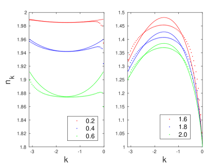
Figure 2: Momentum distribution $n_{k}(L;U)$ for the $1/r$-Hubbard model for $U/W=0.2,0.4,0.6$ in the metallic phase (left), and for $U/W=1.6,1.8,2.0$ in the insulating phase (right) for $-\pi<k<0$. We superimpose the results for the four system sizes $L=16,32,64,128$. Continuous lines in the metallic phase are the predictions from the Gutzwiller wave function (60). Continuous lines in the insulating phase are the predictions from the strong-coupling expansion (73).

For strong coupling, the perturbative result (73) applies (semi-)quantitatively for $U\gtrsim 1.6$ with small deviations around $|k|=\pi/2$, see the right part of Fig. 2. The comparison confirms the validity of the DMRG approach and permits to set the limits for the applicability of the perturbative expressions.

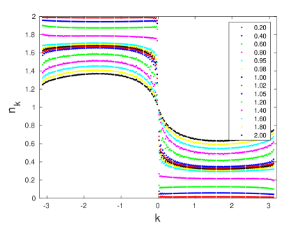
Figure 3: Momentum distribution $n_{k}(L;U)$ for the $1/r$-Hubbard model for $U/W=0.6,0.8,1.0,1.2,1.4$. We superimpose the results for the four system sizes $L=16,32,64,128$.

In Fig. 3 we show the momentum distribution also for intermediate interaction strengths that cannot be accessed from perturbation theory. It is seen that it poses a difficult problem to determine the size of the jump discontinuity from data for finite system sizes.

V Mott-Hubbard transition from finite-size data

In generic one-dimensional Hubbard-type models, the Mott transition at half band-filling occurs at $U_{\rm c}=0^{+}$ because the Umklapp scattering is a relevant perturbation.Giamarchi (2004); Sólyom (2009) Concomitantly, it is exceedingly difficult for the Hubbard model with nearest-neighbor electron transfer to identify the exponentially small gap for small interactions.Lieb and Wu (1968); Gebhard (1997)

In the $1/r$-Hubbard model, the gap is not exponentially small but opens linearly at $U_{\rm c}=W$. It is interesting to see how well the critical interaction can be determined from finite-size data for the single-particle gap and for the momentum distribution.

V.1 Finite-size data for the single-particle gap

The single-particle gap for all system sizes is given by eq. (III.3). The analytical formula shows that the gap scales as

$$\Delta_{1}(L;U\neq U_{\rm c}) = \Delta_{1}(U)+a(U)\frac{1}{L}+{\cal O}\left(\frac{1}{L^{2}}\right)\;,$$ (74)

$$\Delta_{1}(L;U=U_{\rm c}) = a(U_{\rm c})\left(\frac{1}{L}\right)^{1/2}+\frac{3}{4L}+{\cal O}\left(\frac{1}{L^{3/2}}\right)$$

with

$$a(U<U_{\rm c})=\frac{1}{1-U^{2}}\;,\;a(U>U_{\rm c})=1+\frac{U}{U^{2}-1}$$ (75)

and

$$a(U_{\rm c})=2(1-2\sqrt{2})\zeta(-1/2)\approx 0.76021\;.$$ (76)

The analytic behavior of $\Delta_{1}(L;U)$ reflects the fact that the elementary spin excitations of the $1/r$-Hubbard model are gapless with a linear dispersion. The elementary charge excitations also have a finite velocity but with a finite gap in the insulating phase. At the critical interaction, the charge velocity diverges proportional to $1/\sqrt{L}$.Gebhard et al. (1994) In appendix A we perform the standard finite-size analysis of the two-particle gap that does not lead to conclusive results for $U_{\rm c}$.

We follow a different approach and combine the two cases in eq. (V.1) into

$$\Delta_{1}(L;U)=\Delta_{1}(U)+a(U)\left(\frac{1}{L}\right)^{\gamma(U)}$$ (77)

to find

$$\gamma(U)=\begin{cases}\begin{array}[]{@{}lll@{}}1&\text{for}&U\neq U_{\rm c}\\ 1/2&\text{for}&U=U_{\rm c}=1\\ \end{array}\end{cases}\;.$$ (78)

The prefactor $a(U)$ in eq. (V.1) diverges close to the transition,

$$a(U\neq U_{\rm c})\approx\frac{1}{2}\frac{1}{|U-U_{\rm c}|}\;.$$ (79)

Close to the transition, it thus requires system sizes $L\gg 1/|U-U_{\rm c}|$ to reach the asymptotic regime where $\gamma(U)=1$ holds.

In numerical schemes such as the DMRG, we perform calculations for systems with about one hundred sites to keep the numerical effort limited. To extract the gap from finite-size data, we therefore use the form (77) as our interpolation scheme. We denote the numerically obtained values with the upper index “$(L)$”, e.g., $\Delta_{1}^{(L)}(U)$ for the extrapolated finite-size gap and $\gamma^{(L)}(U)$ for the extrapolated exponent when using finite-size data for chains with up to $L$ sites in the extrapolation.

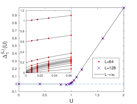
Figure 4: Single-particle gap $\Delta_{1}^{(L)}(U)$ for the $1/r$-Hubbard model as function of $U$, extrapolated from finite-size data with up to $L=64$ sites (points) and $L=128$ site (crosses), respectively. The continuous line is the exact result in the thermodynamic limit, eq. (43). The inset shows the finite-size data and their extrapolation using eq. (77) using the results for up to $L=128$ sites for $U/W=0,0.4,0.6,0.8,0.9,0.95,0.98,1,1.02,1.05,1.1,1.2,1.6,2$. The intercept of the extrapolation curves with the ordinate defines the extrapolation estimate $\Delta_{1}^{(128)}$ for the single-particle gap.

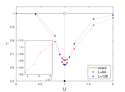
Figure 5: Extrapolation exponents $\gamma^{(64)}(U)$ and $\gamma^{(128)}(U)$ for the $1/r$-Hubbard model as a function of $U/W$. The minimum of the curve determines $U_{\rm c}^{(L)}$.

In Fig. 4 we show the single-particle gap $\Delta_{1}^{(L)}(U)$ for the $1/r$-Hubbard model as a function of $U$ for $L=64,128$. In the inset, we show the finite-size data for $L=16,32,64,128$ sites and the fit of the data to the form (77). It is seen that the extrapolated data $\Delta^{(128)}(U)$ very well reproduce the gap quantitatively but it is not clear how to determine $U_{\rm c}$ accurately because the extrapolated curve $\Delta_{1}^{(L)}(U)$ is smooth and cannot reproduce the kink in the analytical result $\Delta_{1}(U)$ at $U=U_{\rm c}$.

For an accurate estimate of the critical interaction strength, we must use a quantity that very sensitively depends on $U-U_{\rm c}$. As can be seen from eq. (78), the exponent $\gamma(U)$ is such a quantity because it is one half at the critical interaction in comparison to $\gamma(U\neq U_{\rm c})=1$ for all other interaction strengths, see eq. (78). Of course, the isolated discontinuity at $U_{\rm c}$ cannot be reproduced from finite-size studies. However, $\gamma^{(L)}(U)$ retains its minimal value at $U=U_{\rm c}^{(L)}$ that is close to $U_{\rm c}$, see Fig. 5.

Apparently, the minimum of the curve $\gamma^{(L)}(U)$ can be determined very accurately. A quadratic fit in the region $0.95\leq U\leq 1.05$ gives $U_{\rm min}^{(64)}=1.011$ and $U_{\rm min}^{(128)}=1.005$. At $L=128$, the deviation of $U_{\rm c}^{(128)}$ from the exact value $U_{\rm c}=1$ is about five per mille. When we linearly extrapolate the various values for $U_{\rm c}^{(L)}$ for $L=64,96,128$, see the inset of Fig. 5, the exact result can be obtained with an accuracy of $2.5\cdot 10^{-4}$.

The gap exponent can be obtained with a similar precision. As seen from eq. (43), the gap opens linearly as a function of the interaction, $\Delta_{1}(U>U_{\rm c})=(U-U_{\rm c})^{\nu}$ with $\nu=1$. The fit of the gap data for $U\geq 1.02$ gives $\nu^{(128)}=1.003$ ($\nu^{(64)}=0.987$), within three (thirteen) per mille of the exact result.

V.2 Finite-size analysis of the apparent discontinuity in the momentum distribution

Next, we show that the apparent discontinuity of the momentum distribution at the Fermi wave number cannot be used to determine the critical interaction.

In Fig. 6 we show the apparent discontinuity of the momentum distribution,

$$q(L;U) = n_{-\pi/L}(L;U)-n_{\pi/L}(L;U)$$ (80)

$$= 2(n_{-\pi/L}(L;U)-1)\;,$$

where we used particle-hole symmetry in the second step. Inspired by the behavior for strong coupling, we use as our fit function

$$q(L;U)=q(U)+Q_{1}(U)\left(\frac{1}{L}\right)^{\beta(U)}\ln\left(\frac{1}{L}\right)$$ (81)

for the extrapolation to extract $q(U)$. The formula (81) can only apply when $\pi/L$ is rather close to the Fermi edge so that we disregard $L=8,16$ in our fits. The least-square optimization gives $|\beta-1|\ll 1$ for all $U$.

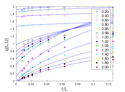
Figure 6: Apparent jump discontinuity $q(L;U)$, eq. (80), for the $1/r$-Hubbard model as a function of $1/L$ for various $U/W$ and $L=8,16,24,32,48,64,96,128$. The lines use the fit function (81).

As seen from Fig 6, the extrapolation from $L=24,32,48,64,96,128$ sites does not produce accurate results for the jump discontinuity. For $U=U_{\rm c}$, the finite-size jump extrapolates to a sizable finite value that persists down to $U=1.2$. For larger values of the interaction, $U\geq 1.2$, the extrapolated gap becomes (slightly) negative. Apparently, the jump discontinuity does not permit to determine the critical interaction strength from system sizes up to $L=128$ sites. System sizes of $L=10^{3}$ or even larger would be required to deduce $U_{\rm c}$ with a reasonable accuracy. Taking into account the scaling of the block entropy for a fixed truncation error, these system sizes are beyond our present computational capacities.

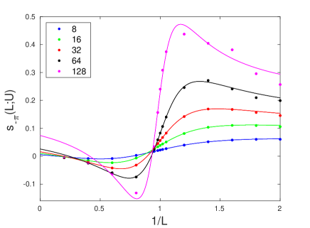
Figure 7: Slope $s_{-\pi}(L;U)$, eq. (82), as a function of $U$ for $L=8,16,32,64,128$. The lines are fits to the Fano function (83).

V.3 Finite-size analysis of band-edge slope

As seen from Figs. 2 and 3, the momentum distribution has (local) extrema at the band edges $k_{\rm B}=\pm\pi$. When we focus on the lower band edge, $n_{\rm\pi-\pi/L}$ displays a (local) minimum in the insulating phase while there is a local maximum or minimum in the metallic phase, depending on the system size. Therefore, it is interesting to analyze the slope of the momentum distribution at the band edge,

$$s_{-\pi}(L;U)=\frac{L}{2\pi}\left[n_{-\pi+\frac{3\pi}{L}}(L;U)-n_{-\pi+\frac{\pi}{L}}(L;U)\right],$$ (82)

as a function of the system size and of the interaction $U$. In Fig. 7 we show the slope $s_{-\pi}(L;U)$ as a function of $U$ for $L=8,16,24,32,48,64,96,128$.

The data resemble points on the curve of a Fano resonance. In appendix B we provide some arguments under which conditions a Fano resonance can show up in the slope $s_{-\pi}(L;U)$,

$$s^{\rm Fano}_{-\pi}(L;U) = a_{-\pi}(L)+\tilde{b}(L)\frac{[\Gamma(L)q_{\rm F}(L)+U-U_{\rm c}(L)]^{2}}{[\Gamma(L)]^{2}+[U-U_{\rm c}(L)]^{2}}$$

(83)

for $|U-U_{\rm c}|\ll U_{\rm c}$. For the five-parameter fit, we use the slope data in the interval $0.4\leq U\leq 1.6$, from the metallic phase into the insulating phase. In Fig. 7 we also display the slope $s^{\rm Fano}_{-\pi}(L;U)$ as a function of $U$ for $L=8,16,32,64,128$. The fits are very good, especially in the vicinity of the critical interaction strength.

In Fig. 8(a) we show the resulting values for $U_{\rm c}(L)$ as a function of $1/L$. They linearly extrapolate to $U_{\rm c}(\infty)=1.004\pm 0.01$, in agreement with the exact value $U_{\rm c}=1$ with an error of about one percent. To achieve a smaller error, we have to increase the system size and the accuracy of the DMRG calculations for $L>64$. It is seen that, for the $1/r$-Hubbard model, the critical interaction can be reliably determined from the slope of the momentum distribution at the lower band edge.

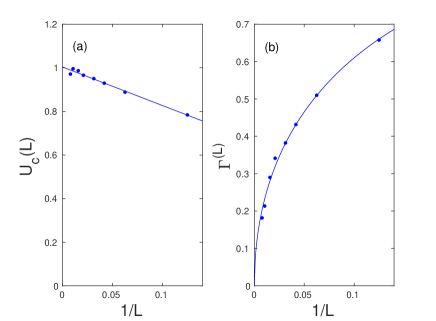
Figure 8: (a) Critical interactions $U_{\rm c}(L)$, eq. (83), seen in the slope $s^{\rm Fano}_{-\pi}(L;U)$, eq. (82), as a function of inverse system size for $L=8,16,24,32,48,64,96,128$. The line is a linear fit in $1/L$. (b) Width $\Gamma^{(L)}$ of the resonance at $U=U_{\rm c}^{(L)}$, eq. (83), seen in the slope $s^{\rm Fano}_{-\pi}(L;U)$, eq. (82), as a function of inverse system size for $L=8,16,24,32,48,64,96,128$. The line is a quadratic fit in $1/\sqrt{L}$.

In Fig. 8(b) we display the width of the resonance $\Gamma(L)$ in eq. (83). The width nicely extrapolates to zero assuming a decay proportional to $1/\sqrt{L}$. As seen for the single-particle gap, eq. (V.1), this scaling is characteristic for the critical interaction. In addition, the extrapolated value confirms that there is a single-particle resonance at the band edge in the thermodynamic limit at $U=U_{\rm c}$.

For completeness, we note that the Fano parameter is almost unity, $q_{\rm F}(L\gtrsim 64)\approx 0.9\pm 0.1$. With the assumption $q_{\rm F}=1$ we have in eq. (83)

$$s^{{\rm Fano},q=1}_{-\pi}(L;U) = a_{-\pi}(L)+\tilde{b}(L)$$

$$+2\tilde{b}(L)\Gamma(L)\frac{U-U_{\rm c}(L)}{[\Gamma(L)]^{2}+[U-U_{\rm c}(L)]^{2}}\;.$$

Since $\Gamma(L)\sim 1/\sqrt{L}$ for large system sizes and $\tilde{b}(L)\Gamma(L)$ must tend to a constant for large system sizes, it is evident that $\tilde{b}(L\gg 1)\sim\sqrt{L}$, as we also confirm numerically. The values $a_{-\pi}(L)$ are negative and diverge for infinite system sizes, $|a_{-\pi}(L)|\sim\sqrt{L}$, because $a_{-\pi}(L)+\tilde{b}(L)$ must remain finite.

Apparently, the slope $s_{-\pi}$ provides a useful method to detect the transition in the $1/r$-Hubbard model. It should be kept in mind that a singular behavior of the slope of the momentum distribution $n_{k}$ at the band edge does not necessarily prove the existence of a metal-insulator transition. We may argue, though, that the occurrence of a single-particle bound state right at the band edge cannot occur in the metallic or in the insulating phase but requires the peculiarities of the transition point between both phases.

VI Conclusions

In this work, we studied the one-dimensional Hubbard model with a linear dispersion relation; the corresponding electron transfer amplitudes decay proportional to the inverse chord distance of two lattice sites on a ring (‘$1/r$-Hubbard model’). Its exact spectrum was conjectured for all system sizes and fillings.Gebhard and Ruckenstein (1992); Gebhard (1997) Using an efficient and accurate density-matrix renormalization group (DMRG) code, we reproduced and thereby confirmed the conjectured energy formula for $L\leq 128$ sites at half band filling (plus one or two particles), with an accuracy of at least six digits for selected $U$-values.

The model provides an ideal case to study the Mott-Hubbard transition numerically because it lacks Umklapp scattering so that the critical interaction occurs at a finite interaction strength, $U_{\rm c}=W$, where $W$ is the bandwidth. Moreover, the single-particle gap opens linearly above the transition, $\Delta_{1}(U\geq W)=U-W$. The critical properties of the spin and charge excitations for this model are fairly simple,Gebhard et al. (1994) so that the finite-size scaling of the single-particle gap permits to locate the critical interaction and the critical exponent with an accuracy of one per mille.

DMRG also allows to calculate ground-state expectation values such as the momentum distribution $n_{k}(L;U)$. For system sizes $L\leq 128$, it is not possible to locate the Mott transition from the apparent jump discontinuity at the Fermi wave vector. Alternatively, we analyze the slope of the momentum distribution at the band edge. It displays a critical behavior at the transition which reflects the formation of a single-particle bound state at the band edge for $U=U_{\rm c}$. Using the slope as a criterion for the Mott transition, the critical interaction can be located only with an accuracy of one percent. Note that the occurrence of a single-particle bound state at the band edges appears to be specific to the $1/r$-Hubbard model.

The main purpose of this work was to study the Mott-Hubbard transition when it is not driven by Umklapp scattering processes, and present alternative approaches to locate quantum phase transitions in many-particle systems when conventional extrapolations, e.g., for the gap, lead to inconclusive results, see appendix A. Moreover, in this work we demonstrated that the DMRG can be used efficiently to carry out the required numerical simulations for large enough systems even for exotic models with long-range complex electron-transfer amplitudes.

Our results open the way to study the Mott transition in one dimension in the presence of long-range interactions. It will be interesting to see how electronic screening in the metal, and its absence in the insulator, modifies the Mott-Hubbard transition. It is not yet clear whether or not the long-range Coulomb interactions alter the Mott-Hubbard transition qualitatively, e.g., whether or not the gap opens continuously when the full screening problem is addressed.Mott (1990) We shall analyze this long-standing open question in a forthcoming publication.

Appendix A Conventional gap extrapolation

For simplicity, we discuss the two-particle gap from eq. (46) because it is given by a simple analytical formula,

$$\Delta_{2}(L;U)=U-U_{\rm c}+\frac{2}{L}+\sqrt{(U_{\rm c}-U)^{2}+\frac{4U}{L}}\;.$$ (85)

As discussed in Sect. II.2, it has the same analytical properties as the single-particle gap. Eq. (85) shows that the gap has a convergent Taylor expansion in $1/L$ if $U\neq U_{\rm c}=W\equiv 1$. Therefore, it seems natural to fit the gap for finite system sizes to the function

$$\Delta_{2}(L;U)\approx\Delta_{2}(U)+a(U)\frac{1}{L}+b(U)\frac{1}{L^{2}}\;.$$ (86)

In Fig. 9(a) we show the extrapolation of the data for $L=8,16,24,32,48,64,96,128$ for $U=0.4,0.8,1,1.2,1.6,2$.

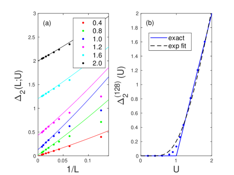
Figure 9: (a) Two-particle gap $\Delta_{2}(L;U)$ as a function of $1/L$ for $L=8,16,32,48,64,96,128$ and $U=0.4,0.8,1,1.2,1.6,2$. The lines are quadratic fits in the inverse system size, see eq. (86). (b) Extrapolated two-particle gap $\Delta_{2}^{(128)}(U)$, for $U=0.2,0.4,0.6,0.8,0.9,1,1.1,1.2,1.4,1.6,1.8,2$, in comparison with the analytic solution in the thermodynamic limit, see eq. (87). The dashed black line shows the fit to eq. (88).

The extrapolation is seen to be very stable and $\Delta_{2}(U)$ can be determined reliably, apart from the critical region where $\delta_{U}(L_{\rm max})=|U-U_{\rm c}|\lesssim 2\sqrt{U_{\rm c}}/\sqrt{L_{\rm max}}$. With $L_{\rm max}=128$ and $U_{\rm c}\approx 1$, we can expect deviations in the region $0.8\lesssim U\lesssim 1.2$. Indeed, as seen from Fig. 9(b), the extrapolation agrees very well with the exact solution in the thermodynamic limit,

$$\Delta_{2}(U\geq U_{\rm c})=\begin{cases}2(U-U_{\rm c})&\text{for}\quad U\geq U_{\rm c}=W\equiv 1\\ 0&\text{for}\quad 0\leq U\leq U_{\rm c}\end{cases}\;,$$ (87)

see eq. (47), outside the region $0.8\lesssim U\lesssim 1.2$.

Inside this region, the continuous but sharp transition at $U_{\rm c}$ is smoothed out. Therefore, it is rather difficult to derive the proper shape of the two-particle gap in the thermodynamic limit. For the present system sizes, even a fit to an exponential form that applies to the exact gap of the standard one-dimensional Hubbard model at small couplings,Essler et al. (2010)

$$\Delta_{2}(U)^{\rm exp}=A\sqrt{U}\exp\left(-\frac{B}{U}\right)\;,$$ (88)

appears to work in the region $0\leq U\leq 2$. The fit with $A=10.28$ and $B=3.905$ is shown as a black dashed line in Fig. 9(b). This fit would incorrectly suggest $U_{\rm c}=0^{+}$ as in the standard Hubbard model.

In order to reduce the size of the critical region by a factor of ten, i.e. down to $\delta_{U}=0.02$, system sizes with $L_{\rm max}=10^{4}$ lattice sites would have to be investigated, $\delta_{U}(10^{4})=0.02$. Such system sizes cannot be treated numerically with the required numerical accuracy now or in the near future. For this reason, the conventional gap extrapolation does not permit to determine $U_{\rm c}$ accurately from numerical data for small system sizes. Therefore, it is important to use the extrapolation scheme introduced in Sect. V.1 that permits an accurate estimate for $U_{\rm c}$ from data for up to $L_{\rm max}=128$ sites.

Appendix B Fano resonance

The Fano-Anderson model describes a localized state coupled to the continuum.Fano (1961); Anderson (1961) It provides a textbook example for which the spectral function can be calculated analytically using Green functions.Mahan (2007) For a Fano resonance at $\epsilon=\epsilon_{0}$, we have

$$A_{\rm Fano}(b,\gamma,q_{\rm F},x)=b\frac{(\gamma q_{\rm F}+x)^{2}}{\gamma^{2}+x^{2}}\;,$$ (89)

where $b$ is the strength of the resonance, $\gamma$ characterizes its width, $q_{\rm F}$ is the Fano parameter, and $x=\epsilon-\epsilon_{0}$ denotes the deviation from the resonance energy. For $q_{\rm F}=1$, the shape of the Fano resonance reduces to

$$A_{\rm Fano}(b,\gamma,q_{\rm F}=1,x) = b+2b\gamma\frac{x}{\gamma^{2}+x^{2}}$$ (90)

$$= b+2b\gamma{\rm Re}\left(\frac{1}{x+{\rm i}\gamma}\right)\;.$$

This explains the counter-intuitive observation that a resonance has the shape of the real part of a level with a finite life-time $\tau=1/\gamma$, instead of its imaginary part.

To motivate the occurrence of a Fano resonance in the slope of the momentum distribution, we assume that the spectral function contains a part where frequency and momentum are related via a dispersion relation,

$$A(k,\omega)=A_{\rm reg}(k,\omega)+A_{\rm F}\left[\omega-v(k+\pi)/(2\pi)-f(U)\right]\;.$$ (91)

Here, we focus on the lower band edge, $|(k+\pi)|\ll\pi$, $v$ is the velocity of the excitations, and $f(U)$ is an unknown function of the interaction that may also depend on the system size. Now that at zero temperature Mahan (2007)

$$n_{k}=\int_{-\infty}^{0}{\rm d}\omega A(k,\omega)\;,$$ (92)

we see that

$$\frac{\partial n_{k}}{\partial k} = \frac{\partial n_{k,{\rm reg}}}{\partial k}-\frac{v}{2\pi}A_{\rm F}\left[-v(k+\pi)/(2\pi)-f(U)\right]\;,$$

where we used that $A(k,-\infty)=0$.Mahan (2007) Setting $k=-\pi$ we obtain

$$s_{-\pi}=a_{-\pi}-\frac{v}{2\pi}A_{\rm F}\left[-f(U)\right]\;,$$ (94)

where we abbreviate $a_{-\pi}=(\partial n_{k,{\rm reg}})/(\partial k)|_{k=-\pi}$.

Since a localized gapless state at the band edge cannot exist but for $U=U_{\rm c}$, we may assume

$$f(U)\approx f_{0}(U-U_{\rm c})$$ (95)

near the critical interaction. We use the Ansatz (95) and eq. (89) in eq. (94) and find after collecting all constants

$$s_{-\pi}(L;U)=a_{-\pi}(L)+\tilde{b}(L)\frac{[\Gamma(L)q_{\rm F}(L)+U-U_{\rm c}(L)]^{2}}{[\Gamma(L)]^{2}+[U-U_{\rm c}(L)]^{2}}$$ (96)

for $|U-U_{\rm c}|\ll U_{\rm c}$, where we made explicit the dependency on the system size when the fit function (96) is applied to finite-size data.

References

- Mott (1990) N. F. Mott, Metal-Insulator Transitions, 2nd ed. (Taylor & Francis, London, 1990).
- Gebhard (1997) F. Gebhard, The Mott Metal-Insulator Transition, Springer Tracts in Modern Physics, Vol. 137 (Springer, Berlin, Heidelberg, 1997).
- Lieb and Wu (1968) E. H. Lieb and F. Y. Wu, Phys. Rev. Lett. 21, 192 (1968).
- Giamarchi (2004) T. Giamarchi, Quantum physics in one dimension, International series of monographs on physics (Clarendon Press, Oxford, 2004).
- Sólyom (2009) J. Sólyom, Fundamentals of the Physics of Solids (Springer, Berlin, 2009) vol. 3.
- Kuramoto (2020) Y. Kuramoto, Quantum Many-Body Physics –A Perspective on Strong Correlations, Lecture Notes in Physics, Vol. 934 (Springer, Heidelberg, Berlin, 2020).
- Gebhard and Ruckenstein (1992) F. Gebhard and A. E. Ruckenstein, Phys. Rev. Lett. 68, 244 (1992).
- Sutherland (1971) B. Sutherland, Journal of Mathematical Physics 12, 251 (1971).
- Sutherland (1985) B. Sutherland, in Exactly Solvable Problems in Condensed Matter and Relativistic Field Theory, Lecture Notes in Physics, Vol. 242, edited by B.S. Shastry, S.S. Jha, and V. Singh (Springer, Berlin, 1985) Chap. 1, p. 1.
- Hubbard (1963) J. Hubbard, Proc. Royal Soc. A 276, 238 (1963).
- Gutzwiller (1963) M. Gutzwiller, Phys. Rev. Lett. 10, 159 (1963).
- Kanamori (1963) J. Kanamori, Prog. Theor. Phys. 30, 275 (1963).
- Mahan (2007) G. D. Mahan, Many particle physics, 3rd ed. (Kluwer Academic/Plenum, New York, Boston, 2007).
- Kuramoto and Yokoyama (1991) Y. Kuramoto and H. Yokoyama, Phys. Rev. Lett. 67, 1338 (1991).
- Schönhammer and Meden (1993) K. Schönhammer and V. Meden, Phys. Rev. B 47, 16205 (1993).
- Voit (1993) J. Voit, Phys. Rev. B 47, 6740 (1993).
- White (1992) S. R. White, Phys. Rev. Lett. 69, 2863 (1992).
- White (1993) S. R. White, Phys. Rev. B 48, 10345 (1993).
- Schollwöck (2005) U. Schollwöck, Rev. Mod. Phys. 77, 259 (2005).
- Szalay et al. (2015) S. Szalay, M. Pfeffer, V. Murg, G. Barcza, F. Verstraete, R. Schneider, and Ö. Legeza, Int. J. Quantum Chem. 115, 1342 (2015).
- McCulloch (2007) I. P. McCulloch, Journal of Statistical Mechanics: Theory and Experiment 2007, P10014 (2007).
- Tóth et al. (2008) A. I. Tóth, C. P. Moca, Ö. Legeza, and G. Zaránd, Phys. Rev. B 78, 245109 (2008).
- Legeza et al. (2003) Ö. Legeza, J. Röder, and B. A. Hess, Phys. Rev. B 67, 125114 (2003).
- Legeza and Sólyom (2004) Ö. Legeza and J. Sólyom, Phys. Rev. B 70, 205118 (2004).
- Wolfram Research, Inc. (2021) Wolfram Research, Inc., Mathematica, Version 12.3 (Wolfram Research, Inc., Champaign, IL, 2021).
- Gebhard and Girndt (1994) F. Gebhard and A. Girndt, Zeitschrift für Physik B Condensed Matter 93, 455 (1994).
- Dzierzawa et al. (1995) M. Dzierzawa, D. Baeriswyl, and M. DiStasio, Phys. Rev. B 51, 1993 (1995).
- Metzner and Vollhardt (1987) W. Metzner and D. Vollhardt, Phys. Rev. Lett. 59, 121 (1987).
- Kollar and Vollhardt (2002) M. Kollar and D. Vollhardt, Phys. Rev. B 65, 155121 (2002).
- Haldane (1988) F. D. M. Haldane, Phys. Rev. Lett. 60, 635 (1988).
- Shastry (1988) B. S. Shastry, Phys. Rev. Lett. 60, 639 (1988).
- Gebhard and Vollhardt (1987) F. Gebhard and D. Vollhardt, Phys. Rev. Lett. 59, 1472 (1987).
- Anderson (1959) P. W. Anderson, Phys. Rev. 115, 2 (1959).
- Gebhard et al. (1994) F. Gebhard, A. Girndt, and A. E. Ruckenstein, Phys. Rev. B 49, 10926 (1994).
- Essler et al. (2010) F. Essler, H. Frahm, F. Göhmann, A. Klümper, and V. Korepin, The one-dimensional Hubbard model (Cambridge University Press, Cambridge, 2010).
- Fano (1961) U. Fano, Phys. Rev. 124, 1866 (1961).
- Anderson (1961) P. W. Anderson, Phys. Rev. 124, 41 (1961).