Commensurate-incommensurate transition in the chiral Ashkin-Teller model

Abstract

We investigate the classical chiral Ashkin-Teller model on a square lattice with the corner transfer matrix renormalisation group (CTMRG) algorithm. We show that the melting of the period-4 phase in the presence of a chiral perturbation takes different forms depending on the coefficient of the four-spin term in the Ashkin-Teller model. Close to the clock limit of two decoupled Ising models, the system undergoes a two-step commensurate-incommensurate transition as soon as the chirality is introduced, with an intermediate critical floating phase bounded by a Kosterlitz-Thouless transition at high temperature and a Pokrovsky-Talapov transition at low temperature. By contrast, close to the four-states Potts model, we argue for the existence of a unique commensurate-incommensurate transition that belongs to the chiral universality class, and for the presence of a Lifshitz point where the ordered, disordered and floating phases meet. Finally, we map the whole phase diagram, which turns out to be in qualitative agreement with the 40 year old prediction by Huse and Fisher.

I Introduction

Recent experiments on Rydberg atoms[1, 2] have brought back the problem of commensurate-incommensurate (C-IC) transitions, and of the nature of the melting of an ordered period-$p$ phase into an incommensurate one. This transition was originally discussed in two dimensional classical systems in the context of the melting of an adsorbed layer on a substrate lattice, and simultaneously introduced by Huse[3] and Ostlund[4] as a series of chiral models exhibiting $p-1$ types of domain walls, such that domain walls between ordered domains $A\mid B$ and $B\mid A$ have different energy, introducing a chiral into the problem. For $p=2$, the system is commensurate even in the disordered phase, and there is no commensurate-incommensurate transition. The transition, if continuous, generically belongs to the Ising universality class. For $p\geq 5$ the transition is always a two-step one, with a critical phase in between. In that phase, the configurations are made of permutations of stripes of the $p$ different orders with domain walls at an average distance of $l\propto 1/q$, where $q$ is the incommensurate wave-vector of the correlations. As the temperature approaches the ordered phase, the domain walls repel each other and the wave-vector converges to a commensurate value with an exponent $\bar{\beta}$ ($q-q_{0}\sim t^{\bar{\beta}}$, where $t=(T-T_{c})/T_{c}$ is the reduced temperature). It is commonly agreed that the transition is in the Pokrovsky-Talapov (PT)[5] universality class, characterised by critical exponents : $\nu_{x}=1/2,\nu_{y}=1,\bar{\beta}=1/2$, where $\nu_{x/y}$ describes the divergence of the correlation length in the directions $x$ and $y$ respectively. The high temperature transition between the critical and the disordered phases is a Kosterlitz-Thouless[6] one driven by the unbinding of the dislocations[7] which become relevant at $\eta=1/4$, where $\eta$ is the exponent of the decay of the spin-spin correlation function.

For the $p=3,4$ cases, the picture might be different. It was first argued by Huse and Fisher [8] that a floating critical phase bounded by two transitions might not appear right away when introducing the chirality. Instead the commensurate-incommensurate transition could be unique and would belong to a new chiral universality class characterised by the product of the correlation length $\xi$ and the wave-vector $q-q_{0}$ converging to a constant at criticality ($\overline{\beta}=\nu$), and by a dynamical (or anisotropy) exponent $z\equiv\nu_{y}/\nu_{x}$ different from 1 ($\nu_{y}\neq\nu_{x}$).

Since its first introduction, the existence of the chiral universality class has generated numerous studies, especially for the $p=3$ case incarnated by the three-state chiral Potts model. Both the classical [9, 8, 10, 11, 12, 13, 14, 15, 16, 17, 18, 19, 20, 21, 22] and quantum [23, 24, 25, 26, 27, 28, 29, 30] cases have been studied extensively. Further experimental work was also performed[31, 32, 33].

By contrast to the $p=3$ case, the $p=4$ literature is less rich. We note however that recently an investigation of a quantum version of the model has suggested the presence of a chiral universality class as well[34]. In this article, we address the $p=4$ case by studying the classical version of the chiral Ashkin-Teller model, and we show that both possibilities (chiral transition or two-step transition) are realized depending on how close one is to the Potts or clock limit of the model.

The paper is organised as follows. In Section II, we describe the model and the different possibilities for the phase diagram. In Section III, we describe the methodology and the CTMRG algorithm. In Section IV, we benchmark the algorithm and discuss its power and limitation. In Section V we present our results. We compare and study in detail the phase diagram of the chiral clock-Ising model, where a floating phase opens right away, and of the four-state chiral Potts model, where we observe a chiral transition, and we propose a full phase diagram of the model.

Figure 1: The two possible phase diagrams for $\lambda<\lambda_{c1}$: either the transition is immediately a two-step one through an intermediate critical floating phase, or it is a direct one in the chiral universality class.

II Chiral Ashkin-Teller model

The 2D Ashkin-Teller model (AT)[35] is defined with two Ising spins $\tau,\sigma\in\{\pm 1\}$ on each site with energy:

$$H_{0}=- \sum_{\langle i,j\rangle}\sigma_{i}\sigma_{j}+\tau_{i}\tau_{j}+\lambda\sigma_{i}\sigma_{j}\tau_{i}\tau_{j}$$ (1)

where the sum runs over pairs of nearest neighbors. It has been shown[36] that there is an exact critical line known from duality where the correlation length exponent varies continuously from the four-state Potts model ($\lambda=1$) to the clock model ($\lambda=0)$ equivalent to two decoupled Ising models as:

$$\nu =\frac{1}{2-\frac{\pi}{2}\arccos(-\lambda)^{-1}}$$ (2)

To our knowledge there is no known theoretical value known for $\bar{\beta}$, but it is believed to be larger than 1, implying that the product $\xi q\rightarrow 0$ along this line[9]. The chiral Ashkin-Teller model can be defined by adding a chiral perturbation along the $x$-direction:

$$H=H_{0}+\Delta\sum_{x,y}(\tau_{x+1,y}\sigma_{x,y}-\sigma_{x+1,y}\tau_{x,y})$$ (3)

This model was originally introduced by Schulz [11], who showed that the chiral perturbation is irrelevant for $\lambda>\lambda_{c_{1}}\sim 0.9779$. For large enough values of $\Delta$, the C-IC transition is expected to be a two-step transition separated by a floating phase. For $\lambda<\lambda_{c_{1}}$, for small enough values of $\Delta$ two possibilities arise, either the transition is two-step and the floating phase opens right away or the transition is unique and belong to the chiral universality class with $\nu_{x}=\bar{\beta}$. The two different scenarios are depicted in Fig. 1. On the other hand, for $\lambda>\lambda_{c_{1}}$, the perturbation is irrelevant, and for small enough values of $\Delta$, the transition is expected to be in the AT universality class. The parameter range between $\lambda_{c_{1}}$ and the Potts limit is very small, actually too small to be observed numerically as we shall see. For larger $\Delta$, beyond this small range of AT transition, the question of a unique chiral transition or a floating phase remains unchanged.

For the rest of the paper, we will refer to the $\lambda=1$ case as the four-state chiral Potts model and to the $\lambda=0$ case as the chiral clock-Ising model in reference to their respective universality classes at $\Delta=0$.

III Methodology

We use the same methodology already developed in the previous work on the three-state chiral Potts model [37] where more details are available.

III.1 CTMRG

The CTMRG algorithm was first introduced by Okunishi and Nishino[38]. It is a numerical method which combines Baxter’s corner matrices[39] and Steve White’s renormalisation group density matrix method[40]. It is most commonly used for two dimensional quantum systems as a contraction algorithm of wave functions[41], but has recently shown promising results on classical systems as well[42, 43, 44].

The investigation of classical systems with tensor networks is done by expressing the partition function in the thermodynamic limit as an infinite tensor network and contracting it. CTMRG sets a way to contract such an infinite square tensor network made of local tensors $a$ on each vertex as shown in Fig. 2. In particular, it allows one to express the Gibbs measure observables as a contraction made of eight tensors denoted by $\mathcal{T}=\{C_{1},T_{1},C_{2},T_{2},C_{3},T_{3},C_{4},T_{4}\}$, with corner tensors $C_{i}$ of dimension $\chi\times\chi$ and row/ column tensors $T_{i}$ of dimensions $\chi\times 4\times\chi$. The parameter $\chi$ is what controls the numerical approximation and is usually referred to as the bond dimension. The local tensors $a$ can be expressed in many different ways, we choose the most common one given by

$$a_{i_{1}i_{2}i_{3}i_{4}}=\sum_{j_{1}j_{2}j_{3}j_{4}}\sqrt{Q_{i_{1}j_{1}}^{x}}\sqrt{Q_{j_{3}i_{3}}^{x}}\sqrt{Q_{i_{2}j_{2}}^{y}}\sqrt{Q_{j_{4}i_{4}}^{y}}$$ (4)

with $Q_{ij}^{x/y}$ the Boltzmann weight matrices between two spins on the horizontal/vertical axis. In the $(\sigma,\tau)=\{(1,1),(1,-1),(-1,1),(-1,-1)\}$ basis, $Q^{x}$ is given by:

$$Q^{x} =\begin{pmatrix}e^{x_{0}}&e^{x_{1}}&e^{x_{2}}&e^{x_{3}}\\ e^{x_{2}}&e^{x_{0}}&e^{x_{3}}&e^{x_{1}}\\ e^{x_{1}}&e^{x_{3}}&e^{x_{0}}&e^{x_{2}}\\ e^{x_{3}}&e^{x_{2}}&e^{x_{1}}&e^{x_{0}}\\ \end{pmatrix}$$ (5)

with

$$x_{0}=\beta(\lambda+2),\quad x_{1}=-\beta(2\Delta+\lambda)$$

$$x_{3}=\beta(\lambda-2),\quad x_{2}=\beta(2\Delta-\lambda))$$

$Q^{y}$ is defined similarly with $\Delta=0$.

Figure 2: Sketch of the partition function as the contraction of a tensor network.

CTMRG therefore provides an easy way to measure directly local observable and two points functions.

The algorithm can be summarised in two steps [45]:

(i) Update: each corner matrix is extended by adding a row, a column and a local $a$ tensor. And each row/ column tensor is extended by adding a local tensor $a$. We illustrate this step for the tensors $C_{1}$ and $T_{1}$ in Fig. 3. The other tensors are updated similarly.

(ii)Truncation: the update increases the bond dimension of the environment tensors by a factor 4. In order to avoid an exponentially growing bond dimension one needs to project the tensors into a subspace. The isometries are given by doing the singular value decomposition on some density matrices and keeping only the $\chi$ largest singular values. The choice of the density matrices influences greatly the convergence of the algorithm. We choose the ones originally proposed by Nishino and Oknishi and given by:

$$\mathcal{U}_{1}^{\prime}\mathcal{S}_{1}^{\prime}\mathcal{V}_{1}^{\prime}=C_{2}^{\prime}C_{3}^{\prime}C_{4}^{\prime}C_{1}^{\prime}$$ (6)

$$\mathcal{U}_{2}^{\prime}\mathcal{S}_{2}^{\prime}\mathcal{V}_{2}^{\prime}=C_{3}^{\prime}C_{4}^{\prime}C_{1}^{\prime}C_{2}^{\prime}$$ (7)

$$\mathcal{U}_{3}^{\prime}\mathcal{S}_{3}^{\prime}\mathcal{V}_{3}^{\prime}=C_{4}^{\prime}C_{1}^{\prime}C_{2}^{\prime}C_{3}^{\prime}$$ (8)

$$\mathcal{U}_{4}^{\prime}\mathcal{S}_{4}^{\prime}\mathcal{V}_{4}^{\prime}=C_{1}^{\prime}C_{2}^{\prime}C_{3}^{\prime}C_{4}^{\prime}$$ (9)

with $C_{i}^{\prime}$ the extended corner matrices. A full iteration for one corner and one column tensor is illustrated in Fig. 3.

Figure 3: Sketch of the full iteration for the corner and row tensors $C_{1}$ and $T_{1}$.

Both steps are repeated until the energy between two iterations converges to some threshold, at which point we consider the thermodynamic limit reached. We note that the initial tensors represent the boundary conditions on the infinite systems and influence the convergence of the algorithm. We choose to set the boundary conditions to be open as it gives the best convergence.

III.2 Effective exponents and critical temperatures

Our analysis is based on effective exponents and some general hypotheses regarding the nature of the transitions. The effective exponent of some physical quantity $A$ which behaves algebraically $A\sim t^{\theta}$ is defined as:

$$\theta_{\text{eff}}=\frac{d\log(A)}{d\log(t)}$$ (10)

with $t=\mid T-T_{c}\mid$, the reduced temperature. Due to crossovers and various corrections, the effective exponent might not be equal to the critical exponent if evaluated outside the critical regime but should converge to it as $t\rightarrow 0$. If the C-IC transition is unique, effective exponents, and in particular $\nu_{\text{eff}}$ from both sides of the transition, should converge to the same value at $t=0$. It turns out that this requirement is enough to fix $T_{c}$. On the other hand, if the transition is two-step, due to the exponential divergence of the correlation length from the KT transition at high temperatures, asking for a unique limit of $\nu_{\text{eff}}$ from both sides of the transition will lead to $\nu>1$. Such an exponent is unphysical and one can conclude that the hypothesis is wrong. Thus, the transition must be two-step. In that case, fixing $T_{KT}$ by looking for the regime where $\eta=1/4$ turned out to be more accurate than fitting the correlation with an exponential, where $\eta$ is the exponent of the decay of the spin-spin correlation function:

$$\langle S_{0}\cdot S_{r}\rangle=\langle\tau_{0}\tau_{r}\rangle+\langle\sigma_{0}\sigma_{r}\rangle\propto r^{-\eta}$$ (11)

$T_{PT}$ is fixed by the condition $\lim_{t\rightarrow 0}\nu_{\text{eff}}^{y}=1$ from the ordered phase. From now on, we will use $\nu^{HT}$ and $\nu^{LT}$ to denote the limit of the effective exponent from the respective high and low temperature regimes.

III.3 Extrapolation of the correlation length and wave-vector

The correlation length and wave-vector can be easily computed through partial diagonalisation of transfer matrices. If one denotes the normalised ordered eigenvalues of the transfer matrix with $\lambda_{i}=\epsilon_{j}e^{i\phi_{j}}$, $j=1,2,\ldots$, then the correlation length and wave-vector are given by:

$$\xi =\frac{1}{\epsilon_{2}},\qquad q=\phi_{2}$$ (12)

This estimation, which corresponds to a given finite bond dimension, can be improved using extrapolations[46] with respect to gaps ($\delta)$ within the transfer matrix spectrum. Rams et al suggested that the inverse correlation length scales linearly such that:

$$\frac{1}{\xi_{\text{exact}}}=\epsilon_{2}+\delta$$ (13)

$$\phi_{\text{exact}}=\phi_{2}+\delta^{\prime}$$ (14)

Various gaps $\delta$ can be used. In particular, in the disordered phase we systematically used $\delta=\epsilon_{4}-\epsilon_{2}$. In some cases the energy levels of the transfer matrices cross and in order to follow a given gap closing, we extrapolate using different eigenvalues. An example of such a case is given in Fig. 4. As for the wave-vector extrapolation, we used differences in the argument of the eigenvalues, usually we used $\delta^{\prime}=\phi_{4}-\phi_{2}$.

Figure 4: Inverse correlation length as function of a gap of the transfer matrix at $\Delta=0.2$ and $\lambda=1$. The bond dimensions used vary from $100$ to $200$. Because of a level crossing, two different eigenvalues were used to extrapolate the correlation in order to follow the same gap : $\delta=\epsilon_{18}-\epsilon_{5}$ (crosses) and $\delta=\epsilon_{16}-\epsilon_{5}$ (circles). Each color represents a different temperature. The simulations are done in the low temperature regime.

III.4 Error bars

The errors on the effective exponents come from the uncertainty on the critical temperature $\delta T_{c}$ and the error in the correlation length from the linear fit $\delta\xi$. A first order Taylor expansion gives:

$$\delta\nu_{\text{eff}}= \nu_{\text{eff}}\left(\frac{\delta\xi(T)}{\xi(T)}+\frac{\delta T_{c}}{T-T_{c}}\right.$$

$$\left.+\frac{\delta\xi(T+dT)+\delta\xi(T-dT)}{\xi(T+dT)-\xi(T-dT)}\right)$$

Error bars on the critical exponents are computed by fitting error bars of the effective exponents as shown in Fig.5

IV Benchmark

In this section we benchmark the results on the two extreme cases $\lambda=0$ and $\lambda=1$ of the well understood Ashkin-Teller line in order to test and understand the limitations of the algorithm. Both models are commensurate along $\Delta=0$, so in order to study $\bar{\beta}$ we approach the critical point from the line $\Delta=T-T_{c}$.

IV.0.1 Ising point

At the $\lambda=\Delta=0$ point, the model decouples into two independent Ising models. Therefore, the transition belongs to the Ising universality class characterised by an exponent $\nu=1$ and a specific heat that diverges logarithmically, i.e. an exponent $\alpha=0$ with a multiplicative logarithmic correction. The critical temperature is known from duality and is given by $T_{c}=2/\log(\sqrt{2}+1)$.

The numerical results are summarised in Fig. 5. A linear extrapolation gives $\nu^{HT}=0.999\pm 0.01$ and $\nu^{LT}=0.992\pm 0.008$ in excellent agreement with the theoretical value $\nu=1$. The wave-vector exponent extrapolates to $\bar{\beta}=1.262\pm 0.004$, implying that the product $\xi q\rightarrow 0$.

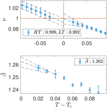
Figure 5: Effective exponents for the Ising model. We extrapolated with a linear fit $\nu=0.992\pm 0.008$ and $\nu=0.999\pm 0.01$ respectively from the low and high temperature regime. The error on the extrapolated values is estimated with a linear fit (grey dashed line) on the error bars of the effective exponents. For $\bar{\beta}$, a linear fit on the last three points extrapolates to $\bar{\beta}=1.262\pm 0.004$.

IV.0.2 Four-state Potts point

We now turn to the $\Delta=0$ and $\lambda=1$ point, which belongs to the four-State Potts universality class. It is characterised by the exponents $\nu=2/3$ and $\alpha=2/3$ with multiplicative logarithm corrections[47] both in the specific heat and in the correlation length. The critical temperature $T_{c}=4/\log 3$ is also known from duality .

Due to these corrections, the measurement of $\nu$ is known to be difficult. In particular, previous studies with the Monte Carlo Renormalization group method[48] have obtained $\nu^{-1}\simeq 1.34$ (or $\nu\simeq 0.746$).We find similar results. A linear extrapolations of the effective exponent on Fig.6 gives $\nu=0.713$. This is quite far from the exact value. Indeed, due to the logarithmic correction, extrapolating the results with a linear fit is wrong and one expects the effective exponent to converge to 2/3 with an infinite slope. We are not close enough to the critical temperature to observe this change of behaviour. For the incommensurability, we observe $\bar{\beta}=1.71\pm 0.02$. Due to the poor accuracy of $\nu$, we can ask how much one can trust this result. However, we notice that the product $\xi q$ has exponent $\bar{\beta}-\nu=0.99\pm 0.06$. Thus, if the product cancels the corrections in the wave-vector and in the correlation length, one would have $\bar{\beta}=2/3+0.99=1.66\pm 0.06$ which we note to be close to the three-state Potts critical exponent. Results are summarised in Fig. 6. In any case, we established that, as expected $\bar{\beta}>\nu$ and $\xi q\rightarrow 0$.

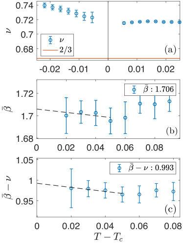
Figure 6: Effective exponents for the Potts model. From top to bottom: (a) Simulations done along the commensurate line; (b)&(c) Simulations done along the line $\Delta\propto T-T_{c}$.

V Results for $0\leq\lambda\leq 1$

We now look at the C-IC transitions. In particular, we study in detail the phase diagram of the chiral Ising and the four-state chiral Potts models. For both systems, we observe a KT and a PT transition enclosing a floating phase. In addition, for the four-state chiral Potts model, we found a unique chiral transition.

V.1 Pokrovsky-Talapov transition

We first consider the $\lambda=0$ model at which we observe a PT transition for $\Delta$ as small as 0.05. As we will see later, in contrast to larger values of $\lambda$, the floating phase extends over a broad parameter range for relatively small values of $\Delta$ and we are able to locate $T_{KT}$ using the criterion $\eta=1/4$ for $\Delta>0.1$. Looking at the phase diagram of Fig. 7, the KT and the PT transitions do not seem to cross before the Ising point and we conclude that, as expected for this model, the floating phase opens up as soon as the chirality is introduced.

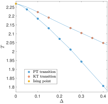
Figure 7: Phase diagram for $\lambda=0$. The red and blue dots represent the measured critical temperatures. The lines are spline interpolations.

In Fig.8, we present a more careful study of the transition at $\Delta=0.4$. We have plotted the inverse correlation length in the $y$-direction and the square of the wave vector with respect to the temperature. We were not able to measure $\xi_{x}$ from the ordered phase due to poor extrapolations. Because in the floating phase the algorithm converges very slowly, the wave-vector values shown have not been extrapolated but were made with fixed bond dimension $\chi=200$ and $\chi=150$. One first notice the accuracy of both linear fits on a large temperature interval, in agreement with critical exponent $\nu_{y}=1$ and $\bar{\beta}=1/2$ with no or very little corrections. If these are indeed the correct critical exponents, the critical temperature can be determined by the intersection with the temperature axis either using the inverse correlation lenght or with the squared wave-vector. This gives respective values of $T_{PT}=1.806$ and $T_{PT}=1.807$, in agreement with each other up to $10^{-3}$, and provides a self consistent picture in agreement with a PT transition. Furthermore, in Fig. 9, we observe that the specific heat does not diverge from the ordered phase but has a clear divergence from the floating phase, as expected at a PT transition.

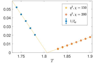
Figure 8: Inverse correlation length and square of the wave-vector as a function of temperature at $\Delta=0.4$ and $\lambda=0$. If $\nu_{y}=1$, $T_{PT}$ can be determined by the intersection of $1/\xi_{y}$ and the temperature axis. If $\bar{\beta}=1/2$, the same applies to the squared wave-vector. The critical temperature extracted from the correlation length gives $T_{PT}=1.806$, and from the wave-vector $T_{PT}=1.807$, both in good agreement with each other. We also plot the squared wave-vector obtained for a smaller bond dimension.

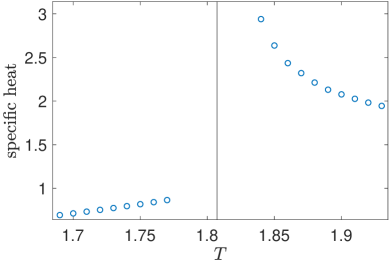
Figure 9: Specific heat at $\Delta=0.4$ and $\lambda=0$ for finite bond dimension, $\chi=200$ at low temperature and $\chi=150$ at high temperature. As there is no extrapolation over the bond dimension, we prefer not to use effective exponents. The specific heat does not diverge from the ordered phase and diverges from the floating phase, as expected for a PT transition.

For $\lambda=1$, we observe a PT transition only at $\Delta>0.7$ with at first, a narrow floating phase. We illustrate the results at $\Delta=0.8$ in Fig. 11. For $\lambda=0$ and $\Delta=0.4$, we deduced $T_{PT}$ from the critical exponents. Here, we work the other way around, we fix $T_{PT}$ and deduce the exponents. Setting $T_{PT}$ with $\nu_{y}^{LT}=1$ at the transition fixes $\bar{\beta}=0.53\pm 0.04$ and $\nu_{x}^{LT}=0.51\pm 0.05$, once again providing a self consistent picture with exponents in good agreement with the PT universality class.

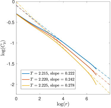
Figure 10: Log-log plot of the spin-spin correlations for $\Delta=0.1$ at $\lambda=0$. The bond dimension used is 200 and the convergence in energy $10^{-9}$. The results are similar up to 400 sites for bond dimension 150. The fits are done between 150 and 300 sites. The exponent reaches the values $\eta=1/4$ between $T=2.22$ and $T=2.225$, allowing us to locate $T_{KT}$ with a precision of the order $5\cdot 10^{-3}$. In general, the larger the floating phase, the slower the exponent $\eta$ varies inside it. Therefore, we have best estimates of the critical temperature for narrow floating phases rather than larger ones.

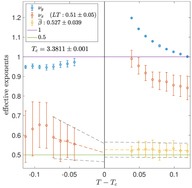
Figure 11: Effective exponents as function of temperature for $\Delta=0.8$ at $\lambda=1$. $\nu_{x}$ and $\nu_{x}$ diverge from the disordered phase in agreement with an exponential divergence of the correlation length. We found $\bar{\beta}=0.53\pm 0.04$ and $\nu_{x}^{LT}=0.51\pm 0.05$. $\bar{\beta}$ is extrapolated with a linear fit on all available points. $\nu_{x}$ is extrapolated with a linear fit on the four last points. The error is computed by fitting the error bars and indicated with a grey dashed line.

V.2 Kosterlitz-Thouless transition

The main limitation of the algorithm is its convergence. It turns out that close to the PT transition, the algorithm does not converge to sufficiently low precision to give sensible results. This forbids us to use the $\eta=1/4$ criteria to determine $T_{KT}$ when the floating phase is too narrow. In that case, an exponential fit of the correlation length will not give enough accuracy to distinguish the two critical temperatures.

As already mentioned, for $\lambda=0$, the floating phase extends over a large parameter range so that even at $\Delta=0.1$ the $\eta=1/4$ criterion can be used to locate the KT transition. We now illustrate such log-log fit with different temperatures in Fig. 10. We notice that the log-log plot is linear only above some threshold distance that increases as the temperature decreases. This is due to the fact that the true power law decay is only visible above the average distance between domain walls $l=\frac{2\pi}{4q}$ which diverges as one approaches the PT transition. For $T=2.22$, we evaluate $\log l\simeq 3.99$ which is in good quantitative agreement of where the curve starts to be linear in Fig. 10. This makes the study of the power law decay close to the transition extremely difficult.

For $\lambda=1$, we can use the $\eta=1/4$ criterion to determine $T_{KT}$ only above $\Delta>1$. In contrast, for $0.7<\Delta<1$ the floating phase is too narrow to distinguish the two critical temperature transitions. In any case we can identify the transition to be in the KT universality class from the divergence of $\nu_{x}$ and $\nu_{y}$ from the high temperature regime at the transition as shown in Fig. 11.

V.3 Chiral transition and Lifshitz point

We now move to $\lambda=1$ and small values of $\Delta$. We recall that at this point, the chiral perturbation is irrelevant and the transition should initially be a unique one in the AT universality class. Yet, we do not see any incommensurate melting in the AT universality class. This is probably due to the fact that the parameter range of the AT transition is too small to be detected by our approach. The results are summarised in Fig.12 and 13. Based on those, we exclude the possibility of a two-step transition. Indeed, fixing the critical temperature up to $10^{-4}$ with a unique exponent $\nu_{y}$ fixes a unique exponent $\nu_{x}$ with good accuracy. We note that both exponents are smaller than one and the transition must then be unique.

For $\Delta=0.3$, we obtained after extrapolation $\nu_{x}^{HT}=0.692\pm 0.012$ and $\nu_{x}^{LT}=0.710\pm 0.010$ in reasonable agreement with each other. Furthermore, we also extrapolated $\bar{\beta}=0.689\pm 0.010$. Then, we obtain $\nu_{x}^{HT}=\bar{\beta}$ within a 0.4% difference, and an anisotrope exponent $z>1$. Those two features are the main characteristics of the chiral universality class and give already strong evidence in favor of a chiral transition. For $\Delta=0.1$, we extrapolate from the disordered phase $\nu_{x}=0.71\pm 0.02$ and $\nu_{y}=0.72\pm 0.03$, close to the effective exponents obtained at the Potts point. Similar exponents are obtained from the ordered phase as shown in Fig. 13. This is probably due to strong crossovers. However, in contrast to the Potts point we extrapolate $\bar{\beta}=0.70\pm 0.02$. Such drastic change of behaviour allows us to conclude that the nature of the transition must be different. Once again, we note that $\nu_{x}^{HT}=\bar{\beta}$ within 1.4% and in agreement with a chiral transition.

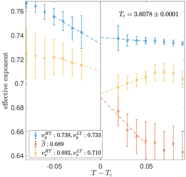
Figure 12: Effective exponents as a function of temperature for $\Delta=0.3$ at $\lambda=1$. Simulations were made with bond dimension between 100 and 200. The main part of the error bars is due to the extrapolations error. Extrapolated exponents come from a linear fit done on the four last points (dashed lined).

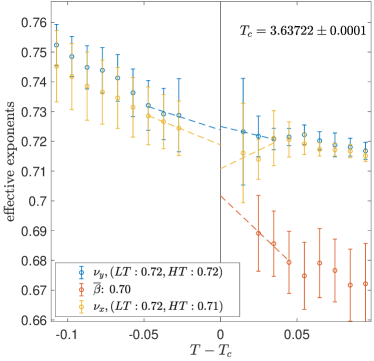
Figure 13: Effective exponents as a function of temperature for $\Delta=0.1$ at $\lambda=1$. Simulations were made with bond dimension between 100 and 200. The main part of the error bars is due to the extrapolations error. Extrapolated exponents come from a linear fit done on the three last points (dashed lined). We obtain, $\nu_{x}^{HT}=0.71\pm 0.02,\nu_{x}^{LT}=0.72\pm 0.01$ and $\bar{\beta}=0.70\pm 0.02$.

As already mentioned, just beyond the Lifshitz point, we will obtain $\nu_{y}>1$ if we try to locate a unique transition due to the KT nature of the upper transition. We can therefore locate the Lifshitz point with the condition $\nu_{y}=1$, leading to a Lifshitz point at $\Delta_{L}=0.705\pm 0.01$.

V.4 Phase Diagram

By applying the same methodology systematically we have been able to map the whole phase diagram, and to identify a line of Lifshitz points. This leads to three different regimes depending on the value of $\lambda$. For $0\leq\lambda<\lambda_{c_{2}}$, the chiral perturbation opens right away a floating phase. By contrast, for $\lambda_{c_{2}}<\lambda<\lambda_{c_{1}}$, the chiral perturbation leads to a unique transition in the chiral universality class, and a floating phase only opens for a non-zero value of $\Delta$. Finally, for $\lambda_{c_{1}}<\lambda\leq 1$, the transition should first be in the AT universality class, a regime too small to be detected numerically. For small but-non zero value of $\Delta$, the transition should become a unique transition in the chiral universality class, and finally, for larger $\Delta$, a floating phase should open. These results are summarised in Fig.14, where we show the three dimensional phase diagram, and in Fig.15, where we show a projection of the phase diagram on the $(\Delta,\lambda)$ plane. The similarity between the phase diagram of Fig.14 and Fig. 12 of Ref. [9] is striking. The transition is clearly unique for a range of $\lambda$ below the Potts point $\lambda=1$, and a two-step one for a range of $\lambda$ above the clock-Ising point $\lambda=0$. A linear extrapolation of the Lifshitz point at $\lambda=0.6$ and $\lambda=0.7$ towards $\Delta=0$ leads to the estimate $\lambda_{c2}\simeq 0.42$, but the curvature of the line of Lifshitz points in Fig. 15 suggests that this value should be considered as an upper bound for $\lambda_{c_{2}}$. This result for $\lambda_{c_{2}}$ is in agreement with recent DMRG simulations on the quantum version of the model[34], for which a chiral transition has been identified in a model with $\lambda\sim 0.57$.

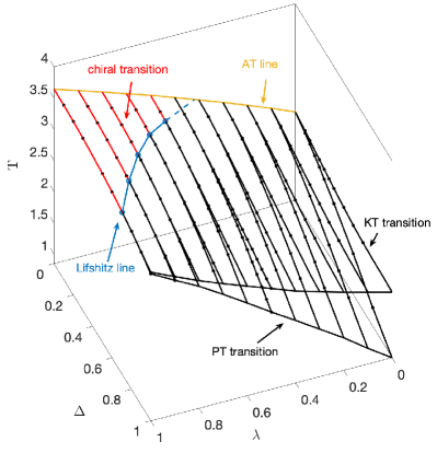
Figure 14: Phase diagram of the chiral Ashkin-Teller model. The orange line is the Ashkin-Teller transition in the absence of a chiral perturbation, while the blue line is the Lifshitz transition. The chiral transition is indicated by red lines. Beyond the Lifshitz line, the commensurate-incommensurate transition becomes a two-step process.

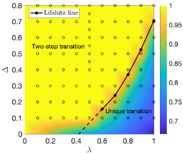
Figure 15: Projection of the phase diagram of the chiral Ashkin-Teller model on the $(\Delta,\lambda)$ plane. The color map shows the critical exponent $\nu_{y}$ from the ordered phase. It is obtained from a linear interpolation of simulations performed at intervals of length 0.1 in the $\Delta$ and $\lambda$ axis (grey dots). In the two-step transition regime, $\nu_{y}=1$ by definition due to the PT nature of the transition. The values along the $\Delta=0$ line are exact. The dotted line is a linear extrapolation of the Lifshitz points at $\lambda=0.6$ and $\lambda=0.7$. It extrapolates to $\lambda\simeq 0.42$.

V.5 Specific heat and Kibble-Zurek exponent

We now discuss and analyse the specific heat exponent $\alpha$ obtained along the line $\lambda=1$ and its relation with the Kibble-Zurek exponent. We recall the hyper-scaling relation $\nu_{x}+\nu_{y}=2-\alpha$. If such a relation applies, there are two different ways to determine if, as reported earlier for the three-state Potts model[37], $\alpha$ is constant along the transition: Either through the direct computation of $\alpha$ itself, or through the computation of the sum $\nu_{x}+\nu_{y}$.

For the Potts point, the exact value is known to be $\alpha=2/3$. Due to logarithmic corrections in the correlation length, we have found $2\nu=1.426$ which gives $\alpha=0.57$. If we make the hypothesis of a chiral transition, we can use the identity $\bar{\beta}=\nu_{x}$ and for $\Delta=0.1$ and $\Delta=0.3$, we respectively found $\nu_{y}^{HT}+\bar{\beta}=1.42$ and 1.427. We also directly studied $\alpha_{\text{eff}}$ (see Fig. 16) and found evidence of a constant exponent along the transition at $\alpha\simeq 0.55$, which establishes the validity of the hyper-scaling relation. Thus, we observe that $\alpha$ seems to be more or less constant along the chiral transition, as already observed in the $p=3$[37] case and in a quantum version of the model at $\lambda\simeq 0.57$[34]. We note that a constant value of $\alpha=2/3$ along the transition and in particular at $\Delta=0$ would imply that there are still logarithmic corrections in the correlation length along the chiral transition. Thus, we are probably overestimating the sum $\nu_{x}+\nu_{y}$, and in fact most certainly $\nu_{x}$ since, in order to keep $\nu_{x}+\nu_{y}=4/3$ with $\nu_{y}>\nu_{x}$, $\nu_{x}$ should be smaller than 2/3.

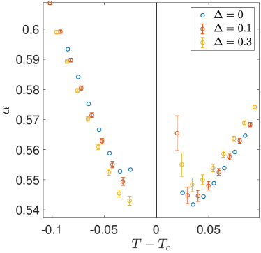
Figure 16: Effective specific heat exponent $\alpha_{\text{eff}}$ for different values of $\Delta$ along the transition at $\lambda=1$. The simulation are performed at finite $\chi=200$. The error bars for $\Delta=0.1$ and $\Delta=0.3$ come from the uncertainty of the critical temperature.

The Kibble-Zurek exponent can be measured in arrays of Rydberg atoms[2]. It is defined as $\mu=\nu/(1+\nu z)$, with $\nu$ the correlation length exponent along the chain and $z$ the dynamical exponent. In our case, $z$ plays the role of the anisotropy exponent $z=\nu_{y}/\nu_{x}$, and $\nu$ is the correlation length exponent in the $x$-direction. Therefore, we can compute the Kibble-Zurek exponent as $\mu=\nu_{x}/(1+\nu_{y})$. For reasons discussed above, we choose to express $\mu$ with respect to $\nu_{y}$. Then, using the hyper-scaling relation and the hypothesis of a constant $\alpha=2/3$ along the transition, the Kibble-Zurek exponent becomes $\mu=(4/3-\nu_{y})/(1+\nu_{y})$. Using this expression of the exponent and the critical exponents obtained from the disordered phase for $\lambda=1$, we found $\mu=0.36$ and $\mu=0.34$ for $\Delta=0.1$ and $\Delta=0.3$ respectively. These results indicate that the Kibble-Zurek exponent is smaller along the chiral transition than at the Potts point, where $\mu=0.4$. These results are in qualitative agreement with recent experiments[2] on chains of Rydberg atoms, which have been argued to be described by the AT model with $\lambda$ close to 1 in the vicinity of the $p=4$ ordered phase[34], and for which values $\mu\simeq 0.25$ have been reported[2] .

VI Results for $\lambda\notin[0,1]$

Since our main purpose was to identify a possible chiral transition we have concentrated in the preceding section on the interval $\lambda\in[0,1]$ since it contains the relevant parameter range $\lambda_{c2}\lesssim 0.32\leq\lambda<\lambda_{c1}=0.9779$. For completeness we now comment on the effect of a chiral perturbation outside this interval.

VI.1 $-1<\lambda<0$

In this range, the chiral perturbation stays relevant and the floating phase open up as soon as the chirality is introduced. The zero temperature ground state stays four times degenerate and we do not expect any qualitative change from the $\lambda<\lambda_{c2}$ case.

VI.2 $\lambda<-1$

In this case, at $\Delta=0$, the nature of the zero temperature ground state has changed and so has the transition. It is expected to be described by Ising critical exponents. Indeed, in the $\lambda\rightarrow\infty$ limit, the model is described by Ising variables $u_{i}=\tau_{i}\sigma_{i}$ and the hamiltonian reduces to $H=\sum_{i\sim j}u_{i}u_{j}$. The zero temperature ground state is infinitely degenerate and we recover a $\log(2)$ residual entropy. Introducing the chirality will lift the residual entropy but the zero temperature ground state stays $2^{L}$ degenerate for a $L\times M$ lattice size, and we expect the transition to stay a C-C one. We thus also expect the transition to stay in the Ising universality class. Other values of $\lambda$ within the interval should be described by the same physics. We show results for $\lambda=-2$ at finite chirality $\Delta=0.1$ in Fig. 17. And as expected we found a unique $\pi$ commensurate - $\pi$ commensurate transition with a correlation length exponent consistent with the Ising value $\nu=1$.

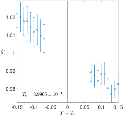
Figure 17: Evidence of a unique transition at $\lambda=-2$ and $\Delta=0.1$ with a critical exponent $\nu$ in good agreement with the Ising universality class $\nu=1$. For this simulation, we have changed the isometries and used those in[45], which we noticed to perform better in the anisotropic case.

VI.3 $\lambda>1$

At $\Delta=0$, for $\lambda>1$, the self dual line does not represent the critical line anymore and the Ashkin-Teller transition splits up into two Ising transitions with in between a nematic phase characterised by $\langle\tau_{1}\sigma_{1}\rangle\neq 0$. When introducing the chirality, the two Ising transitions first stay in the Ising universality class but as the chirality increases, the nematic phase closes and the two Ising transitions merge into a unique one bounded by commensurate phases, as illustrated in Fig.18 for $\lambda=1.7$. Upon further increasing the chirality $\Delta$, the high temperature phase becomes incommensurate, and for large enough $\Delta$ a floating phase bounded by KT and PT transitions appears. For this value of $\lambda$, the range of chiral transition (if any) is too small to be detected. By contrast, for not too large $\lambda$, we found evidence for the existence of a chiral transition to follow up on the AT one. This result is illustrated in Fig. 19. In the high chirality limit, one recovers a two-step transition separated by a floating phase (not shown). Based on the results illustrated in Fig. 18 and 19, a sketch of the expected generic phase diagram as a function of $\Delta$ is shown in Fig. 20. Whether the chiral transition persists for all $\lambda$ is an open question that would require further investigation.

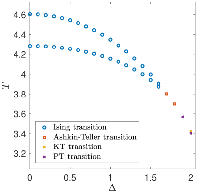
Figure 18: Phase diagram at $\lambda=1.7$ (above the Potts point) as a function of $\Delta$. The two Ising transitions at small $\Delta$ merge around $\Delta\simeq 1.7$ into a single phase transition that must be in the AT universality class since the high temperature phase remains commensurate for some range of $\Delta$. At larger $\Delta$, a floating phase bounded by KT and PT transitions develop. For this value of $\lambda$, the region of chiral transition (if any) is too small to be detected.

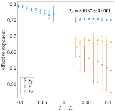
Figure 19: Evidence of a unique transition with $\bar{\beta}\simeq\nu_{x}$ for $\lambda=1.05$ and $\Delta=0.5$, in agreement with a chiral transition.

Figure 20: Sketch of the expected generic phase diagram for $\lambda>1$. The high-temperature phase above the Ising and AT transitions is commensurate. The width of the various phases varies with $\lambda$, and the widths of the sketch are arbitrary. Upon increasing $\lambda$, the width of the chiral transition becomes smaller and smaller to the point where we cannot say for sure if it still exists.

VII Summary

Based on the qualitative study of effective exponents, we have been able to give a self consistent picture of the critical exponents and universality classes, and to identify two different types of commensurate-incommensurate transitions, either a two-step one through a KT and a PT transition, or a unique chiral transition. If we take for granted that for $\lambda_{c_{1}}\simeq 0.9779\leq\lambda\leq 1$, the transition should remain AT for a while, something we have not been able to show numerically because this range is too small, we are led to the conclusion that the Ashkin-Teller family of models can be classified into three regimes according to the way they react to a chiral perturbation: (i) A floating phase opens right away for $0\leq\lambda<\lambda_{c_{2}}$; (ii) The transition is unique in the chiral universality class for $\lambda_{c_{2}}\leq\lambda<\lambda_{c_{1}}$; (iii) The transition remains in the AT universality class before becoming chiral for $\lambda_{c_{1}}\leq\lambda\leq 1$. The critical value for $\lambda_{c_{2}}$ could not be pinned down very precisely, but it can be expected to satisfy $\lambda_{c_{2}}\lesssim 0.42$. We further found evidence for the chiral transition to be characterised by a specific heat exponent that keeps its AT value. In many models, the melting of an ordered period-4 phase into incommensurate phase takes place and the nature of the transition is still debated. If an Ashkin-Teller point is present along the transition, by identifying its universality class and its exponent $\nu$, our prediction can be used to determine the nature of the melting close to that point. Further study on such a model and in particular on the quantum chiral Ashkin-Teller model would be of particular interest to test these predictions.

Acknowledgments. We thank Natalia Chepiga and Jeanne Colbois for useful discussions. This work has been supported by the Swiss National Science Foundation. The calculations have been performed using the facilities of the Scientific IT and Application Support Center of EPFL.

References

- Bernien et al. [2017] H. Bernien, S. Schwartz, A. Keesling, H. Levine, A. Omran, H. Pichler, S. Choi, A. S. Zibrov, M. Endres, M. Greiner, V. Vuletic, and M. D. Lukin, Probing many-body dynamics on a 51-atom quantum simulator, Nature 551, 579 (2017).
- Keesling et al. [2019] A. Keesling, A. Omran, H. Levine, H. Bernien, H. Pichler, S. Choi, R. Samajdar, S. Schwartz, P. Silvi, S. Sachdev, P. Zoller, M. Endres, M. Greiner, Vuletić, V. , and M. D. Lukin, Quantum Kibble-Zurek mechanism and critical dynamics on a programmable Rydberg simulator, Nature 568, 207 (2019).
- Huse [1981] D. A. Huse, Simple three-state model with infinitely many phases, Phys. Rev. B 24, 5180 (1981).
- Ostlund [1981] S. Ostlund, Incommensurate and commensurate phases in asymmetric clock models, Phys. Rev. B 24, 398 (1981).
- Pokrovsky and Talapov [1979] V. L. Pokrovsky and A. L. Talapov, Ground state, spectrum, and phase diagram of two-dimensional incommensurate crystals, Phys. Rev. Lett. 42, 65 (1979).
- Kosterlitz and Thouless [1973] J. M. Kosterlitz and D. J. Thouless, Ordering, metastability and phase transitions in two-dimensional systems, Journal of Physics C: Solid State Physics 6, 1181 (1973).
- José et al. [1977] J. V. José, L. P. Kadanoff, S. Kirkpatrick, and D. R. Nelson, Renormalization, vortices, and symmetry-breaking perturbations in the two-dimensional planar model, Phys. Rev. B 16, 1217 (1977).
- Huse and Fisher [1982] D. A. Huse and M. E. Fisher, Domain walls and the melting of commensurate surface phases, Phys. Rev. Lett. 49, 793 (1982).
- Huse and Fisher [1984] D. A. Huse and M. E. Fisher, Commensurate melting, domain walls, and dislocations, Phys. Rev. B 29, 239 (1984).
- Schulz [1980] H. J. Schulz, Critical behavior of commensurate-incommensurate phase transitions in two dimensions, Phys. Rev. B 22, 5274 (1980).
- Schulz [1983] H. J. Schulz, Phase transitions in monolayers adsorbed on uniaxial substrates, Phys. Rev. B 28, 2746 (1983).
- Cardy [1993] J. L. Cardy, Critical exponents of the chiral potts model from conformal field theory, Nuclear Physics B 389, 577 (1993).
- Au-Yang and Perk [1996a] H. Au-Yang and J. H. Perk, Phase diagram in the generalized chiral clock models, Physica A: Statistical Mechanics and its Applications 228, 78 (1996a).
- Yeomans and Derrida [1985] J. Yeomans and B. Derrida, Bulk and interface scaling properties of the chiral clock model, Journal of Physics A: Mathematical and General 18, 2343 (1985).
- Sato and Sasaki [2000a] H. Sato and K. Sasaki, Numerical study of the two-dimensional three-state chiral clock model by the density matrix renormalization group method, Journal of the Physical Society of Japan 69, 1050 (2000a).
- Selke and Yeomans [1982] W. Selke and J. M. Yeomans, A monte carlo study of the asymmetric clock or chiral potts model in two dimensions, Zeitschrift für Physik B Condensed Matter 46, 311 (1982).
- Duxbury et al. [1984] P. M. Duxbury, J. Yeomans, and P. D. Beale, Wavevector scaling and the phase diagram of the chiral clock model, Journal of Physics A: Mathematical and General 17, L179 (1984).
- Sato and Sasaki [2000b] H. Sato and K. Sasaki, Numerical study of the two-dimensional three-state chiral clock model by the density matrix renormalization group method, Journal of the Physical Society of Japan 69, 1050 (2000b), https://doi.org/10.1143/JPSJ.69.1050 .
- Houlrik and Jensen [1986] J. M. Houlrik and S. J. K. Jensen, Phase diagram of the three-state chiral clock model studied by monte carlo renormalization-group calculations, Phys. Rev. B 34, 325 (1986).
- Au-Yang and Perk [1996b] H. Au-Yang and J. H. Perk, Phase diagram in the generalized chiral clock models, Physica A: Statistical Mechanics and its Applications 228, 78 (1996b).
- Au-Yang et al. [1987] H. Au-Yang, B. M. McCoy, J. H. Perk, S. Tang, and M.-L. Yan, Commuting transfer matrices in the chiral potts models: Solutions of star-triangle equations with genus¿1, Physics Letters A 123, 219 (1987).
- Baxter et al. [1988] R. Baxter, J. Perk, and H. Au-Yang, New solutions of the star-triangle relations for the chiral potts model, Physics Letters A 128, 138 (1988).
- Howes [1983] S. F. Howes, Commensurate-incommensurate transitions and the lifshitz point in the quantum asymmetric clock model, Phys. Rev. B 27, 1762 (1983).
- Chepiga and Mila [2019] N. Chepiga and F. Mila, Floating phase versus chiral transition in a 1d hard-boson model, Phys. Rev. Lett. 122, 017205 (2019).
- Samajdar et al. [2018] R. Samajdar, S. Choi, H. Pichler, M. D. Lukin, and S. Sachdev, Numerical study of the chiral quantum phase transition in one spatial dimension, Phys. Rev. A 98, 023614 (2018).
- Everts and Roder [1989] H. U. Everts and H. Roder, Transfer matrix study of the chiral clock model in the hamiltonian limit, Journal of Physics A: Mathematical and General 22, 2475 (1989).
- Zhuang et al. [2015] Y. Zhuang, H. J. Changlani, N. M. Tubman, and T. L. Hughes, Phase diagram of the parafermionic chain with chiral interactions, Phys. Rev. B 92, 035154 (2015).
- Howes et al. [1983] S. Howes, L. P. Kadanoff, and M. D. Nijs, Quantum model for commensurate-incommensurate transitions, Nuclear Physics B 215, 169 (1983).
- Whitsitt et al. [2018] S. Whitsitt, R. Samajdar, and S. Sachdev, Quantum field theory for the chiral clock transition in one spatial dimension, Phys. Rev. B 98, 205118 (2018).
- Centen et al. [1982] P. Centen, V. Rittenberg, and M. Marcu, Non-universality in z3 symmetric spin systems, Nuclear Physics B 205, 585 (1982).
- Bartelt et al. [1987] N. C. Bartelt, T. L. Einstein, and L. D. Roelofs, Structure factors associated with the melting of a (31) ordered phase on a centered-rectangular lattice gas: Effective scaling in a three-state chiral-clock-like model, Phys. Rev. B 35, 4812 (1987).
- Abernathy et al. [1994] D. L. Abernathy, S. Song, K. I. Blum, R. J. Birgeneau, and S. G. J. Mochrie, Chiral melting of the si(113) (3×1) reconstruction, Phys. Rev. B 49, 2691 (1994).
- Schreiner et al. [1994] J. Schreiner, K. Jacobi, and W. Selke, Experimental evidence for chiral melting of the ge(113) and si(113) 3×1 surface phases, Phys. Rev. B 49, 2706 (1994).
- Chepiga and Mila [2021] N. Chepiga and F. Mila, Kibble-zurek exponent and chiral transition of the period-4 phase of rydberg chains, Nature Communications 12, 414 (2021).
- Ashkin and Teller [1943] J. Ashkin and E. Teller, Statistics of two-dimensional lattices with four components, Phys. Rev. 64, 178 (1943).
- Kohmoto et al. [1981] M. Kohmoto, M. den Nijs, and L. P. Kadanoff, Hamiltonian studies of the ashkin-teller model, Phys. Rev. B 24, 5229 (1981).
- Nyckees et al. [2021] S. Nyckees, J. Colbois, and F. Mila, Identifying the huse-fisher universality class of the three-state chiral potts model, Nuclear Physics B 965, 115365 (2021).
- Nishino and Okunishi [1996] T. Nishino and K. Okunishi, Corner transfer matrix renormalization group method, J. Phys. Soc. Jpn. 65, 891 (1996).
- Baxter [1982] R. J. Baxter, Exactly solved models in statistical mechanics (1982).
- White [1992] S. R. White, Density matrix formulation for quantum renormalization groups, Phys. Rev. Lett. 69, 2863 (1992).
- Corboz et al. [2007] P. Corboz, A. M. Läuchli, K. Totsuka, and H. Tsunetsugu, Spontaneous trimerization in a bilinear-biquadratic zig-zag chain, Phys. Rev. B 76, 220404 (2007).
- Ueda et al. [2020a] H. Ueda, K. Okunishi, S. Yunoki, and T. Nishino, Corner transfer matrix renormalization group analysis of the two-dimensional dodecahedron model, Phys. Rev. E 102, 032130 (2020a).
- Ueda et al. [2020b] H. Ueda, K. Okunishi, K. Harada, R. Krčmár, A. Gendiar, S. Yunoki, and T. Nishino, Finite- scaling analysis of berezinskii-kosterlitz-thouless phase transitions and entanglement spectrum for the six-state clock model, Phys. Rev. E 101, 062111 (2020b).
- Krcmar et al. [2016] R. Krcmar, A. Gendiar, and T. Nishino, Phase diagram of a truncated tetrahedral model, Phys. Rev. E 94, 022134 (2016).
- Orús and Vidal [2009] R. Orús and G. Vidal, Simulation of two-dimensional quantum systems on an infinite lattice revisited: Corner transfer matrix for tensor contraction, Phys. Rev. B 80, 094403 (2009).
- Rams et al. [2018] M. M. Rams, P. Czarnik, and L. Cincio, Precise extrapolation of the correlation function asymptotics in uniform tensor network states with application to the bose-hubbard and xxz models, Phys. Rev. X 8, 041033 (2018).
- Salas and Sokal [1997] J. Salas and A. D. Sokal, Logarithmic corrections and finite-size scaling in the two-dimensional 4-state potts model, Journal of Statistical Physics 88, 567 (1997).
- Eschbach et al. [1981] P. D. Eschbach, D. Stauffer, and H. J. Herrmann, Correlation-length exponent in two-dimensional percolation and potts model, Phys. Rev. B 23, 422 (1981).