Edge-featured Graph Neural Architecture Search

Abstract

Graph neural networks (GNNs) have been successfully applied to learning representation on graphs in many relational tasks. Recently, researchers study neural architecture search (NAS) to reduce the dependence of human expertise and explore better GNN architectures, but they over-emphasize entity features and ignore latent relation information concealed in the edges. To solve this problem, we incorporate edge features into graph search space and propose Edge-featured Graph Neural Architecture Search (EGNAS) to find the optimal GNN architecture. Specifically, we design rich entity and edge updating operations to learn high-order representations, which convey more generic message passing mechanisms. Moreover, the architecture topology in our search space allows to explore complex feature dependence of both entities and edges, which can be efficiently optimized by differentiable search strategy. Experiments at three graph tasks on six datasets show EGNAS can search better GNNs with higher performance than current state-of-the-art human-designed and searched-based GNNs.

1 Introduction

Architecture design is a critical component of successful deep learning. Lately, the neural architecture search (NAS) baker2016designing ; liu2018darts ; pham2018efficient ; zhang2021automated ; zoph2016neural has been extensively studied to explore the optimal network architectures and lessen the manual intervention. Most NAS works baker2016designing ; liu2018darts ; pham2018efficient ; zoph2016neural focus on searching architectures about CNN and RNN. Recently, graph neural networks (GNNs) have become standard toolkits for analyzing complex graph-structure data, facilitating many relational tasks such as chemical molecular property prediction, social network analysis and recommendation. However, only a few efforts cai2021rethinking ; zhang2021automated conceive NAS in graph machine learning domain. In this paper, we study edge-featured graph neural architecture search to improve GNN’s reasoning capability.

The core of GNNs is the message passing mechanism, which learns graph representation by propagating feature information between neighboring entities. This helps capture the semantic context implied in the graph. Unlike image and sequence data, which have a grid structure, graph data lies in a non-Euclidean space bronstein2017geometric , leading to unique architectures and designs for graph machine learning. Typical search space of CNN/RNN NAS focuses on improving the representation learning capability by combining convolution, pooling and activation operations. Differently, graph search space aims to explore effective message passing mechanisms, which is the key challenge to solve graph neural architecture search problem.

Currently graph search spaces can be divided into two categories: macro- and micro-space. Macro search space gao2020graph ; jiang2020graph is constructed using popular GNNs (e.g. GIN xu2018powerful , GAT velivckovic2017graph ) as atom operations, which is actually a kind of GNN ensemble and represents limited message passing models. Micro search space consists of fine-grained atomic operations such as neighbor aggregation, feature filtering and combining function cai2021rethinking ; zhang2021automated , that hold promise for discovering novel message passing mechanisms. The existing graph NAS methods mainly focus on learning effective entity embeddings, but ignore the latent high-order information associated with edges. In fact, mining the relation information concealed in the edges can guide fine-grained message passing on graph and enrich graph search space, which is beneficial to node-level, edge-level and graph-level tasks.

Recently, increasing manually-designed GNNs chen2021edge ; jiang2019censnet ; Li_2019_CVPR ; yang2020nenn try to incorporate edge features into models for better exploiting relation information. Specifically, they stack the building layers in a sequential architecture and iteratively learn features of entity and edge. Nevertheless, such plain architecture follows incremental updating rule based on current layer’s representation, which is naive and sub-optimal. Also, these approaches adopt simple edge learning function, which is difficult to learn high-order and long-term relation features.

In this paper, we propose Edge-featured Graph Neural Architecture Search (EGNAS) with novel edge-featured search space to learn the optimal GNN architecture using gradient-based search strategy. Our search space (shown in Figure 1(b)) treats edge as entity-equivalent and adopts dual updating graph as architecture topology to learn the high-order representations of entity and edge, which presents more generic message passing mechanisms. Specifically, it models multi levels of entity and edge features, and allows complex dependence among them rather than classical sequential structure. Further, we design two kind of atomic operations: (1) entity updating operations for aggregating neighboring messages guided by relation features, (2) edge updating operations for modeling higher order relations guided by entity features. Based on the differentiable search algorithm, we can efficiently find the optimal dependence graph and updating operations to construct final GNN. Experiments at six benchmarks show our EGNAS can search better GNNs with higher performance than current state-of-the-art methods, including hand-designed and searched-based GNNs.

Our contributions can be summarized as follows:

• We present edge-featured graph neural architecture search to find the optimal graph neural architecture, where a novel search space is designed with rich entity and edge updating operations.

• This is the first effort that explicitly incorporates edge features into graph search space, where dual updating graph is introduced to explore complex entity/edge feature dependence and learn high-order representations, presenting more generic message passing mechanisms.

• We evaluate EGNAS on six benchmarks at three typical graph tasks. The results show that graph architectures searched by EGNAS outperform the human-invented and search-based architectures.

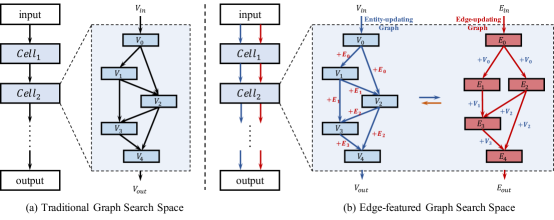
Figure 1: A comparison between the traditional cell-based graph search space and our proposed edge-featured graph search space with dual updating graph of entity and edge.

2 Related Work

Graph Neural Networks. GNNs have been successfully applied to operate on the graph-structure data bresson2017residual ; brockschmidt2020gnn ; corso2020principal ; kipf2016semi ; li2015gated ; NEURIPS2020_1534b76d ; velivckovic2017graph ; vignac2020building ; xu2018powerful ; yang2020factorizable . Current GNNs are constructed on message passing mechanisms and can be categorized into two groups, isotropic and anisotropic. Isotropic GNNs hamilton2017inductive ; kipf2016semi ; li2015gated ; vignac2020building ; xu2018powerful aim at extending the original convolution operation to graphs. Anisotropic GNNs enhance the original models with anisotropic operations on graphs perona1990scale , such as gating and attention mechanism battaglia2016interaction ; bresson2017residual ; marcheggiani2017encoding ; monti2017geometric ; velivckovic2017graph ; yang2020factorizable . Anisotropic methods usually achieve better performance, since they can adaptively weight the edges according to the entity features and guide the message passing. However, these methods over-emphasize on entity rather than edge features.

Exploiting Edge Features. Recently, researchers chen2021edge ; jiang2019censnet ; Li_2019_CVPR ; schlichtkrull2018modeling ; yang2020nenn have tried to intergrate edge features into GNN architecture. Schlichtkrull et al. schlichtkrull2018modeling propose R-GCNs to model relational data by grouping edges on graph, which indicates the edges cannot include continuous attributes. Works chen2021edge ; jiang2019censnet ; yang2020nenn assign high-dimensional feature for edges and iteratively update edge features using the same way as entity updating. These methods take no account of the dependencies between multi-level relation features and lack of diversified update functions to compute the edge features.

Neural Architecture Search. NAS aims at finding the optimal nerural architectures specific to dataset baker2016designing ; cai2018proxylessnas ; chu2020darts ; li2020sgas ; liang2019darts+ ; liu2018darts ; pham2018efficient ; xie2018snas ; zoph2016neural . Search space and search strategy are the most essential components in NAS. Search space defines which architectures can be represented in principal. Search strategy details how to explore the search space. Methods can be mainly categorized into three groups, reinforcement learning (RL) baker2016designing ; zoph2016neural ; zoph2018learning , evolutionary algorithms (EA) liu2017hierarchical ; real2019regularized ; real2017large and gradient-based (GB) liu2018darts ; xu2019pc ; zela2019understanding . Due to the success in CNNs and RNNs, recent researchers cai2021rethinking ; gao2020graph ; jiang2020graph ; lai2020policy ; nunes2020neural ; zhang2021automated ; zhou2019auto apply NAS in graph machine learning domain to automatically design GNNs, termed as graph neural architecture search. Most of these works mainly focus on designing graph search space that can process non-euclidean data. However, during designing search space, they all ignore the information associated with edges that can be beneficial to graph tasks. To our best knowledge, we are the first to explicitly model edge features in graph NAS problem.

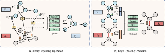
Figure 2: Illustration of entity updating operation and edge updating operation. “F” module in subfigure (a) is used for processing messages based on feature-wise linear modulating operation before aggregating.

3 Method

In this section, we first formulate the problem of graph neural architecture search, then introduce edge-featured graph search space and entity/edge updating operations. Next, we discuss the gradient-based search algorithm. Finally, we describe how to design final layers based on the specific task.

3.1 Problem Statement

We formally define the graph neural architecture search as following bi-level optimization problem. Given graph search space $\mathcal{A}$, we aim to find the optimal GNN architecture $\alpha^{*}\in\mathcal{A}$ that minimizes the validation loss $\mathcal{L}_{val}(w^{*}(\alpha),\alpha^{*})$. The trainable weights $w^{*}$ associated with the architecture are obtained by minimizing the training loss $\mathcal{L}_{train}(w^{*},\alpha^{*})$. Mathematically, it is written as follows.

$${\alpha}^{*} =\mathop{argmin}\limits_{\alpha\in\mathcal{A}}\mathcal{L}_{val}(w^{*}(\alpha),\alpha)$$ (1)

$$w^{*}(\alpha) =\mathop{argmin}\limits_{w}\mathcal{L}_{train}(w,\alpha)$$ (2)

The characteristic of GNN search problem is that the search space $\mathcal{A}$ consists of atomic operations which are designed to process complex graph-structure data and convey rich message passing mechanisms.

3.2 Search Space

Similar to the search space of CNNs, we search computational cells as the building blocks and stack them for the final model (shown in Figure 1(b)). In our edge-featured search space, each computational cell consists of dual directed acyclic graphs, termed as entity-updating graph and edge-updating graph. In the following, we will describe how the two graphs are constructed.

Entity-updating Graph. Entity-updating graph consists of an ordered sequence of $N$ nodes. Each node $\bm{V}_{i}$ is latent representations (i.e. entity embeddings in a GNN layer) and each directed edge $(i,j)$ is associated with some entity-updating operation $o_{\mathcal{V}}^{(i,j)}$ that transforms $\bm{V}_{i}$ to $\bm{V}_{j}$ guided by relation features $\bm{E}_{i}$ (shown in Figure2(a)). We compute each imtermediate node based on all its predecessors, written as

$$\bm{V}_{j}=\sum_{0\leq i<j}o_{\mathcal{V}}^{(i,j)}(\bm{V}_{i},\bm{E}_{i}),$$ (3)

where $1\leq j\leq N$, $\bm{V}_{0}$ denotes the input entity representation. Inspired by works brockschmidt2020gnn ; perez2018film , we use relation representation as input that determines an element-wise affine transformation of incoming messages. This allows the model to dynamically up-weight and down-weight features based on the information of relation. It yields the following update rule,

$$\bm{\beta}^{(s,t)},\bm{\gamma}^{(s,t)}=g(\bm{E}^{(s,t)}_{i};\bm{\theta}_{i}),$$ (4)

$$\bm{V}_{j}^{(t)}=\mathcal{M}(\{\bm{\gamma}^{(s,t)}\odot\bm{V}_{j}^{(s)}+\bm{\beta}^{(s,t)}|s\in\mathcal{N}(t)\}),$$ (5)

where $g(\cdot)$ is a function to compute affine transformation, $\bm{\theta}_{i}$ is learnable parameters, $\mathcal{N}(t)$ denotes neighboring entities of target entity $t$. We define optional message aggregator $\mathcal{M}(\cdot)$ as a continuous function of multisets that aggregates messages on neighboring entities, such as $\mathop{sum}$, $\mathop{mean}$ and $\mathop{max}$. Different aggregators capture different types of information, work cai2021rethinking demonstrates that $\mathop{sum}$, $\mathop{mean}$, and $\mathop{max}$ do well in capturing structural, statistical and representative information from neighboring entities, respectively. Our search space allows to select the most appropriate message aggregators for different graph datasets. Besides, we introduce entity skip-connect operation in search space to alleviate the gradient vanishing and over-smoothing problems. The output of the whole entity-updating graph is obtained by applying a reduction operation (e.g. concatenation) to all the intermediate nodes.

Edge-updating Graph. Edge-updating graph is a directed acyclic graph with the same number of nodes but different topology as entity-updating graph. Each node $\bm{E}_{i}$ is the latent relation representation and each directed edge $(i,j)$ is associated with some edge-updating operation $o^{(i,j)}_{\mathcal{E}}$ that learns higher order relation representation $\bm{E}_{j}$ from both $\bm{E}_{i}$ and its corresponding entity representation $\bm{V}_{i}$ (shown in Figure2(b)). Similarly, the intermediate node in edge-updating graph follows below update rule,

$$\bm{E}_{j}=\sum_{0\leq i<j}o_{\mathcal{E}}^{(i,j)}(\bm{E}_{i},\bm{V}_{i}),$$ (6)

where $1\leq j\leq N$, $\bm{E}_{0}$ denotes the input relation representation. Note that, if there is no original relation representation in datasets, then $\bm{E}_{0}$ is initialized with identity vectors $\bm{1}=[1]$. Specifically, for two entities $s$ and $t$, we first compute the joint entity representation as temporary relation feature $[\bm{V}^{(s)}_{i}\parallel\bm{V}^{(t)}_{i}]$, then use it to update current relation representation $\bm{E}^{(s,t)}_{i}$:

$$\bm{E}^{(s,t)}_{j}=\mathcal{U}(\bm{E}^{(s,t)}_{i},[\bm{V}^{(s)}_{i}\parallel\bm{V}^{(t)}_{i}])$$ (7)

where $\parallel$ denotes concatenation operation, $\mathcal{U}(\cdot,\cdot)$ is an optional updating function. To present more message passing mechanisms, we introduce several update functions with different capabilities, such as Concat, FiLM perez2018film and GRU chung2014empirical . Concat denotes concatenation, that is the naivest operation of feature aggregation. FiLM is short for feature-wise linear modulation that dynamically up-weight or down-weight old relation feature guided by temporary relation feature. GRU adaptively determines how much old relation feature to forget and how much temporary relation features to inject. This is critical for preserving long-term relation and constructing robust high-order relation features. Besides, we also introduce a special operation edge skip-connect to improve learning deep relation features. The output of the edge-updating graph is also obtained by applying a reduction operation to all the intermediate nodes.

3.3 Search Strategy

Following previous works cai2021rethinking ; li2020sgas , we adopt differentiable NAS strategy to find the optimal GNN. Instead of optimizing different operations separately, differentiable strategy maintains a supernet (one-shot model) containing all candidate operations, formally written as

$$\bar{o}^{(i,j)}(x)=\sum_{o\in\mathcal{O}}\frac{exp(\alpha^{(i,j)}_{o})}{\sum_{o^{\prime}\in\mathcal{O}}exp(\alpha^{(i,j)}_{o^{\prime}})}o(x),$$ (8)

where $\mathcal{O}$ is a set of candidate operations, $\alpha^{(i,j)}$ is learnable vector that controls which operation is selected. Briefly, each mixed operation $\bar{o}^{(i,j)}$ is regarded as a probability distribution of all possible operations. In this way, we can use gradient-based algorithms to jointly optimize the architecture and model weights. At the end of search, a discrete architecture is derived from supernet by replacing each mixed operation $\bar{o}^{(i,j)}$ with the most likely operation, i.e., $o^{(i,j)}=\mathop{argmax}_{o\in\mathcal{O}}\alpha^{(i,j)}_{o}$. For each node in cell, we retain at most two edges from all of its incoming edges. $\mathcal{O}$ can either be entity updating operation set $\mathcal{O}_{\mathcal{V}}$ or edge updating operation set $\mathcal{O}_{\mathcal{E}}$.

3.4 Task-based Layer

We design the final network layers depending on the specific task. Let $\mathcal{V}=\{v_{1},v_{2},...,v_{|\mathcal{V}|}\}$ be the set of entities and $\mathcal{E}\subseteq\mathcal{V}\times\mathcal{V}$ be the set of edges, $\bm{V}_{o}\in\mathbb{R}^{|\mathcal{V}|\times d_{\mathcal{V}}},\bm{E}_{o}\in\mathbb{R}^{|\mathcal{E}|\times d_{\mathcal{E}}}$ be the final entity representation and edge (relation) representation, respectively.

Node-level task layer. For node classification task, the prediction $\bm{y}^{(i)}_{\mathcal{V}}$ is done as follows:

$$\bm{y}^{(i)}_{\mathcal{V}}=\bm{P}_{\mathcal{V}}\bm{V}^{(i)}_{o}$$ (9)

where $\bm{P}_{\mathcal{V}}\in\mathbb{R}^{C\times d_{\mathcal{V}}}$ is the classifier, $C$ is the number of entity classes.

Edge-level task layer. For edge classification task, our method naturally makes predictions based on deep edge features $\bm{E}_{o}$, formally written as

$$\bm{y}^{(s,t)}_{\mathcal{E}}=\bm{P}_{\mathcal{E}}\bm{E}^{(s,t)}_{o}$$ (10)

where $\bm{P}_{\mathcal{E}}\in\mathbb{R}^{C\times d_{\mathcal{E}}}$ is a learnable matrix, $C$ is the number of edge classes. This is better than traditional GNN works kipf2016semi ; xu2018powerful ; velivckovic2017graph that concatenate the entity features as edge features, since the independent edge features are more discriminative at edge-level tasks.

Graph-level task layer. For graph classification and regression tasks, we first use mean-pooling readout operation to compute global entity feature and global edge feature, then concatenates them as global graph representation. The prediction $\bm{y}_{\mathcal{G}}$ is computed as follows

$$\bm{y}_{\mathcal{G}}=\bm{P}_{\mathcal{G}}\big{[}\frac{1}{|\mathcal{V}|}\sum_{i\in\mathcal{V}}\bm{V}^{(i)}_{o}\big{|}\big{|}\frac{1}{|\mathcal{E}|}\sum_{(s,t)\in\mathcal{E}}\bm{E}^{(s,t)}_{o}\big{]},$$ (11)

where $\bm{P}_{\mathcal{G}}\in\mathbb{R}^{C\times(d_{\mathcal{V}}+d_{\mathcal{E}})}$ is a learnable transformation matrix, $C$ is the number of graph classes.

4 Experiments

4.1 Experimental Setups

Datasets. We evaluate our method on six datasets (TSP, ZINC irwin2012zinc , MNIST lecun1998gradient , CIFAR10, PATTERN dwivedi2020benchmarking and CLUSTER dwivedi2020benchmarking ) across three different level tasks (edge-level, graph-level and node-level). TSP dataset is based on the classical Travelling Salesman Problem, which tests edge classification on 2D Euclidean graphs to indentify edges belonging to the optimal TSP solution. ZINC is one popular real-world molecular dataset of 250K graphs, whose task is graph property regression, out of which we select 12K for efficiency following works cai2021rethinking ; corso2020principal ; dwivedi2020benchmarking . MNIST and CIFAR10 are original classical image classification datasets and converted into graphs using superpixel achanta2012slic algorithm to test graph classification task. PATTERN and CLUSTER are node classification tasks generated via Stochastic Block Models abbe2017community , which are used to model communications in social networks by modulating the intra-community and extra-community connections. Details about the six datasets are shown in Table LABEL:tab_summary, where $\mathcal{V},\mathcal{E},\mathcal{G}$ denote node-level, edge-level and graph-level tasks, respectively.

Searching settings. In EGNAS, we define entity updating operation set $\mathcal{O}_{\mathcal{V}}$: sum, max, mean, entity skip-connect and zero, edge updating operation set $\mathcal{O}_{\mathcal{E}}$: Concat, GRU, FiLM, edge skip-connect and zero. Unless otherwise stated, each operation except skip-connect and zero is followed by a FC-ReLU-BN module. For fair comparison, on MNIST and CIFAR10, the search space consists of one computational cell. For other datasets, the search space consists of 4 cells. Each cell consists of 4 entity features and 4 edge features. In order to stablelize the gradient, additional residual connections are introduced in each computational cell. To carry out the architecture search, we hold out half of the training data as validation set. The supernet is trained using EGNAS for $40$ epochs, with batch size $64$ (for both the training and validation set). We use momentum SGD to optimize the weights $\bm{w}$, with initial learning rate $\eta_{\bm{w}}=0.025$ (anneald down to zero following a cosine schedule without restart), momentum $0.9$, and weight decay $3\times 10^{-4}$. We use Adam kingma2014adam as the optimizer for $\bm{\bm{\alpha}}$, with initial learning rate $\eta_{\alpha}=3\times 10^{-4}$, momentum $\beta=(0.5,0.999)$ and weight decay $10^{-3}$.

Training settings. For fair comparison, we follow all training settings (data splits, optimizer, metrics, etc) in work cai2021rethinking ; dwivedi2020benchmarking . Specifically, we adopt Adam kingma2014adam with the same learning rate decay for all runs. The learning rate is initialized with $10^{-3}$, which is reduced by half if the validation loss stop decreasing after 10 epochs. During training on CIFAR10 and MNIST dataset, we set dropout to 0.2 to alleviate the overfitting. For MNIST and CIFAR10 datasets, we report the results of state-of-the-art GNNs with 4 layers. According to the searching settings, for other datasets, the GNNs with 16 layers are compared. These experiments (including searching and training) are run on NVIDIA GTX 2080Ti. Additional details can be found in the supplementary materials.

4.2 Results of Graph-level Task

To test the capacity of our method at graph-level tasks, we assess it on MNIST, CIFAR10 (both are graph classification task) and ZINC (graph regression task) datasets. The experimental results are reported in Table LABEL:tab_graph and Table LABEL:tab_ZINC_TSP. We observe that, first, our method surpasses all the state-of-the-art hand-designed and search-based GNNs by a large margin ($17.5\%\uparrow$ on ZINC, $3.8\%\uparrow$ on CIFAR10, $0.3\%\uparrow$ on MNIST), which demonstrates the effectiveness of EGNAS. Compared with the previous GNAS approaches cai2021rethinking ; gao2020graph , our EGNAS achieves a great performance improvement with fewer parameters. This indicates that our designed search space with more efficient atomic operations is better than traditional graph search space, and the searched GNN has more compact graph architecture. Second, the performance of EGNAS without edge features degrades significantly, proving that exploiting relation information in edges is critical for learning better graph representations. Even on CIFAR10 and MNIST datasets whose edges only describe binary topological connections, our EGNAS still mines latent relation to guide better message passing on graph.

4.3 Results of Edge-level Task

We compare the performance of our optimal searched architecture with state-of-the-art hand-designed and search-based GNNs on TSP dataset. The results are presented in Table LABEL:tab_ZINC_TSP. We observe that GNNs incorporating edge features significantly outperform those only focusing on learning entity features, where the latter velivckovic2017graph ; cai2021rethinking obtain the representation of edges for final classification by concatenating entity features. This indicates that at the task of edge classification, assigning independent features to each edge can reduce its dependence on the entity features, and thus improve the discriminability of edge representations. In addition, the optimal GNN architecture discovered by our EGNAS surpasses the state-of-the-art GatedGCN bresson2017residual , which reflects the effectiveness of EGNAS at edge-level tasks. The performance improvement benefits from that our dual updating graph facilitates to explore more generic message passing mechanisms.

4.4 Results of Node-level Task

We show the results at node classification task on PATTERN and CLUSTER datasets in Table LABEL:tab_node. PATTERN dataset tests the fundamental graph task of recognizing specific predetermined subgraphs, and the CLUSTER dataset aims at identifying community clusters, where structural information matters. Notably, the graphs in these datasets represent community networks, in which the edge only plays role in connecting two nodes. Interestingly, we find that our EGNAS still achieves competitive performance on PATTERN and surpasses all the state-of-the-art GNNs on CLUSTER. Actually, the message propagation through intra-community and extra-community connections should be different on CLUSTER. The GNNs searched by EGNAS can still distinguish intra-community and extra-community connections through mining local structural similarities between nodes. Specifically, they model structural similarity information in edge features using edge updating operations, to guide message passing and help identify specific communities on graph.

4.5 Ablation Study for Architectures

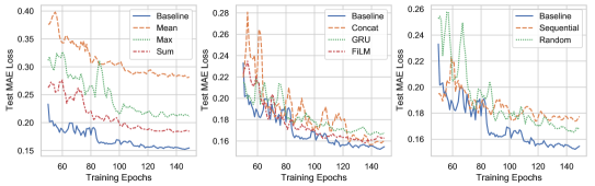
Figure 3: Experiments of modifying searched GNN architecture on ZINC dataset. Baseline architecture is the best GNN architecture searched by the EGNAS, the others are obtained by modifying baseline architecture based on different rules, such as replacing entity updating operation (left), edge updating operation (middle) and modifying architecture topology (right).

Here, we explore what happens if we make some changes to the optimal searched architecture, which is termed as “Baseline” architecture. First, we study the impact of the replacement of atomic operations. Specifically, we replace all the entity updating operations in “Baseline” architecture with a specific operation (e.g. Mean, Max, Sum), with other operations unchanged, obtaining three modified architectures. Similarly, we replace all the edge updating operations in “Baseline” architecture with Conat, GRU and FiLM operations, respectively, for ablations of edge updating operations. These six architectures are retrained on ZINC dataset and the test performance in terms of MAE is shown in Figure 3 (left and middle). We can observe that both convergence speed and MAE of the modified architectures are worse than the “Baseline” architecture, which means that the representation ability of a single feature updating operation is limited. Further, our method can automatically search the optimal way to combine different entity/edge updating operations, discovering novel message passing mechanisms and enhancing the graph representation learning capability of GNN.

Second, we study the impact of architecture topology (feature dependence graph). We randomly sample a graph neural architecture from edge-featured graph search space, termed as “Random”. Besides, we obtain a “Sequential” architecture by removing some edges from edge-updating graph of “Baseline” architecture to make sure that $\bm{E}_{i}$ just depends on $\bm{E}_{i-1}$. Experimental results (the right of Figure 3) show that “Random” is better than “Sequential” but worse than “Baseline” architecture. This emphasizes that searching complex dependence graph of multi-level edge features matters. It is also interesting to note that randomly sampled architecture is competitive, which reflects the importance of the graph search space design.

Figure 4: Best architecture with 4 cells searched on ZINC dataset. Each subfigure corresponds to a specific computational cell, in which the above and below graphs describe edge-updating graph and entity-updating graph, respectively. Notably, entity updating operations with $(+\bm{E}_{x})$ means the architecture updates entity features guided by edge features $\bm{E}_{x}$. Similar, edge updating operations with $(+\bm{V}_{x})$ denotes that the entity features $\bm{V}_{x}$ are involved in the computation of learning edge features.

4.6 Further Discussion

According to the experiments, we have observed some interesting phenomena that may inspire the design of edge-featured GNNs. The longest path in the edge updating graph is getting shorter as the computational cell depth increases (more nodes directly connect to $\bm{E}_{0}$ with edge skip-connect operation). As depth increases, the edge features are smoothed along with entity features, weakening the ability to characterize the local structural similarity. Our EGNAS can automatically detect this phenomenon and supplement some lower order edge features via extra connections to counteract this smoothness. Another evidence is that the “Sequential” architecture performs worse than “Baseline” architecture (shown in the right of Figure 3), where “Baseline” contains more connections from lower order edge features in deeper computational cells. The searched architectures on other datasets also show similar preference. More results can be found in supplementary materials.

5 Conclusion

In this paper, we incorporate edge features in graph neural architecture search for the first time, to find the optimal GNN architecture that can mine and exploit latent relation information concealed in edges. Specifically, we design edge-featured graph search space with novel atomic operations, which allows to explore complex entity/edge feature dependence and presents more generic message passing mechanisms. Experiments on six benchmarks at three classical graph tasks demonstrate that our EGNAS rivals all the human-invented and search-based methods. Further, we analyze the searched optimal architectures and confirm the effectiveness of our EGNAS.

Boarder Impact

Our paper proposes edge-featured graph neural architecture search method that further introduces novel graph search space with more generic message passing mechanisms and find the optimal GNN architecture. Notably, this is a significant improvement on designing graph search space. It will have a direct impact on the application of graph neural networks in the industry. The positive impacts are described as follows. First, we can efficiently find better GNN architectures that can mine and exploit the relation information implied in graph. So the practical application of GNN to the corresponding area can be fostered. Second, we analyze the optimal searched GNN architectures and summarize some findings which may have implications for the design of GNN. Moreover, by applying our EGNAS to different tasks and datasets, we think that it could bring researchers expertise in understanding graph neural architectures. There are also some limitations in our method. For example, we mainly focus on designing generic graph search space rather than search strategy. We will develop specific search strategies for graph neural architecture search to improve the efficiency and performance of search in future works.

Appendix A Implementation Details

In this section, we details how entity updating operations and edge updating operations are formulated. We declare that $\bm{V}\in\mathbb{R}^{|\mathcal{V}|\times d_{\mathcal{V}}}$ denotes entity feature, $\bm{E}\in\mathbb{R}^{|\mathcal{E}|\times d_{\mathcal{E}}}$ denotes edge feature, $\mathcal{V}$ is the set of entities, $\mathcal{E}$ is the set of edges, $d_{\mathcal{V}}$ is the dimension of entity feature, $d_{\mathcal{E}}$ is the dimension of edge feature.

A.1 Entity Updating Operation

As discussed in body content, we use relation representation as input that determines an element-wise affine transformation of incoming messages, allowing the model to dynamically up-weight and down-weight features based on the information of relation. It yields the following update rule,

$$\bm{\beta}^{(s,t)},\bm{\gamma}^{(s,t)}=g(\bm{E}^{(s,t)}_{i};\bm{\theta}_{i}),$$ (12)

$$\bm{V}_{j}^{(t)}=\mathcal{M}(\{\bm{\gamma}^{(s,t)}\odot\bm{V}_{j}^{(s)}+\bm{\beta}^{(s,t)}|s\in\mathcal{N}(t)\}),$$ (13)

where $g(\cdot)$ is a function to compute affine transformation, $\bm{\theta}_{i}$ is learnable parameters, $\mathcal{N}(t)$ denotes neighboring entities of target entity $t$, $\mathcal{M}$ is an optional neighbor aggregator. We define Max, Mean, Sum entity updating operations for aggregating messages, with neighbor aggregator $\mathcal{M}(\cdot)$ as $max(\cdot)$, $mean(\cdot)$ and $sum(\cdot)$, respectively. Besides, we also introduce a special operation entity skip-connect to alleviate the gradient vanishing and over-smoothing problems, formulated as

$$o_{\mathcal{V}\cdot skip}(\bm{V}_{i},\bm{E}_{i})=\bm{V}_{i}.$$ (14)

A.2 Edge Updating Operation

As we discussed in body content, the edge updating equation can be written as follows:

$$\bm{E}^{(s,t)}_{j}=\mathcal{U}(\bm{E}^{(s,t)}_{i},[\bm{V}^{(s)}_{i}\parallel\bm{V}^{(t)}_{i}])$$ (15)

where $\parallel$ denotes the concatenation operation, $\mathcal{U}(\cdot,\cdot)$ is an optional updating function. Since we define multiple edge updating operations Concat, GRU, FiLM and edge skip-connect, the difference between them is the choice of the updating function $\mathcal{U}(\cdot,\cdot)$.

For Concat Operation. Concat denotes the concatenation, that is the naivest operation of feature aggregation. We use the following updating rule:

$$\mathop{\mathcal{U}}\limits_{Concat}(\bm{E}^{(s,t)}_{i},[\bm{V}^{(s)}_{i}\parallel\bm{V}^{(t)}_{i}])=MLP([\bm{E}^{(s,t)}_{i}\parallel\bm{V}^{(s)}_{i}\parallel\bm{V}^{(t)}_{i}])$$ (16)

where $MLP(\cdot)$ denotes a multi-layer perceptron that obtains new edge feature with $d_{\mathcal{E}}$ dimension.

For GRU Operation. GRU [12] adaptively determines how much old relation feature to forget and how much temporary relation features to inject. This is critical for preserving long-term relation and constructing robust high-order relation features. Mathematically, it can be formulated as

$$\bm{x}=ReLU(\bm{P}_{x}[\bm{V}^{(s)}_{i}\parallel\bm{V}^{(t)}_{i}])$$ (17)

$$\bm{r}=\sigma(\bm{U}_{r}\bm{x}+\bm{W}_{r}\bm{E}^{(s,t)}_{i})$$ (18)

$$\bm{z}=\sigma(\bm{U}_{z}\bm{x}+\bm{W}_{z}\bm{E}^{(s,t)}_{i})$$ (19)

$$\bm{h}=tanh(\bm{U}_{h}\bm{x}+\bm{W}_{h}(\bm{r}\odot\bm{E}^{(s,t)}_{i}))$$ (20)

$$\mathop{\mathcal{U}}\limits_{GRU}(\bm{E}^{(s,t)}_{i},[\bm{V}^{(s)}_{i}\parallel\bm{V}^{(t)}_{i}])=(\bm{1}-\bm{z})\odot\bm{E}^{(s,t)}_{i}+\bm{z}\odot\bm{h}$$ (21)

where $\bm{P}_{x}\in\mathbb{R}^{d_{\mathcal{E}}\times 2d_{\mathcal{V}}}$, $\bm{U}_{r}\in\mathbb{R}^{d_{\mathcal{E}}\times d_{\mathcal{E}}}$, $\bm{W}_{r}\in\mathbb{R}^{d_{\mathcal{E}}\times d_{\mathcal{E}}}$, $\bm{U}_{z}\in\mathbb{R}^{d_{\mathcal{E}}\times d_{\mathcal{E}}}$, $\bm{W}_{z}\in\mathbb{R}^{d_{\mathcal{E}}\times d_{\mathcal{E}}}$, $\bm{U}_{h}\in\mathbb{R}^{d_{\mathcal{E}}\times d_{\mathcal{E}}}$ and $\bm{W}_{h}\in\mathbb{R}^{d_{\mathcal{E}}\times d_{\mathcal{E}}}$ are learnable matrices, $ReLU$ is ReLU activation function, $\sigma(\cdot)$ is sigmoid activation function.

For FiLM Operation. FiLM is short for feature-wise linear modulation [33] that dynamically up-weight or down-weight old relation feature guided by temporary relation feature. The required updating function can be written as

$$\bm{\beta}^{(s,t)},\bm{\gamma}^{(s,t)}=g([\bm{V}^{(s)}_{i}\parallel\bm{V}^{(t)}_{i}];\bm{\theta}_{i})$$ (22)

$$\mathop{\mathcal{U}}\limits_{FiLM}(\bm{E}^{(s,t)}_{i},[\bm{V}^{(s)}_{i}\parallel\bm{V}^{(t)}_{i}])=\bm{\gamma}^{(s,t)}\odot\bm{E}^{(s,t)}_{i}+\bm{\beta}^{(s,t)}$$ (23)

where $g(\cdot)$ is a function to compute affine transformation, $\bm{\theta}_{i}$ is learnable parameters.

For edge skip-connect Operation. We introduce a special operation edge skip-connect to improve learning deep relation features, formulated as

$$\mathop{\mathcal{U}}\limits_{skip-connect}(\bm{E}^{(s,t)}_{i},[\bm{V}^{(s)}_{i}\parallel\bm{V}^{(t)}_{i}])=\bm{E}^{(s,t)}_{i}$$ (24)

The skip-connect plays role in supplementing low level representations and alleviating gradient vanishing.

Appendix B Architecture Visualization

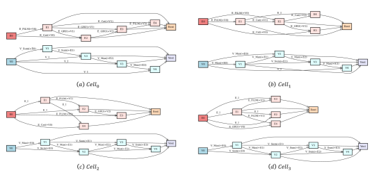
Figure 5: Best architecture with 4 cells searched on ZINC dataset.

As a supplementary for Section 4.6 in body content, we visualize the best searched architecture for each dataset, including ZINC (shown in Figure 5), TSP (shown in Figure 6), CLUSTER (shown in Figure 7), PATTERN (shown in Figure 8), MNIST (shown in Figure 9[a]) and CIFAR10 (shown in Figure 9[b]). The visualization results on these datasets show similar preference as discussed in Section 4.6, i.e., as depth increases, the edge features are smoothed along with entity features, weakening the ability to characterize the local structural similarity. Our EGNAS can automatically detect this phenomenon and supplement some lower order edge features via extra connections to counteract this smoothness.

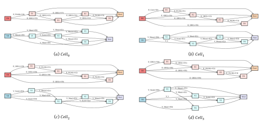
Figure 6: Best architecture with 4 cells searched on TSP dataset.

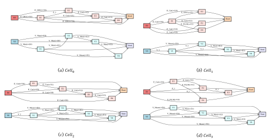
Figure 7: Best architecture with 4 cells searched on CLUSTER dataset.

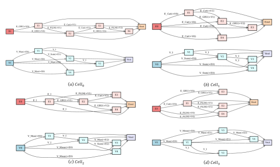
Figure 8: Best architecture with 4 cells searched on PATTERN dataset.

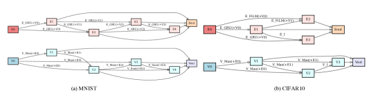
Figure 9: Best architecture with one cell searched on MNIST and CIFAR10 datasets.

Appendix C Extensive Experiments

To evaluate the sensitivity of our method to the size of the receptive field, we conduct extensive experiments at edge-level task (on TSP dataset) and graph-level task (on ZINC dataset), then report the results in Table LABEL:tab_ZINC_TSP_ex. Besides, we also conduct extensive experiments at node-level task (no both PATTERN and CLUSTER datasets) and report the results in Table LABEL:tab_node_ex. We can find that, with the increase of receptive field, the performance of our model becomes better and better. Our method can achieve competitive results in any receptive field. In addition, through the ablation studies, we can see that incorporating edge features into search space is critical for improving performance of searched GNN architectures.

References

- [1] Emmanuel Abbe. Community detection and stochastic block models: recent developments. The Journal of Machine Learning Research, 18(1):6446–6531, 2017.
- [2] Radhakrishna Achanta, Appu Shaji, Kevin Smith, Aurelien Lucchi, Pascal Fua, and Sabine Süsstrunk. Slic superpixels compared to state-of-the-art superpixel methods. IEEE transactions on pattern analysis and machine intelligence, 34(11):2274–2282, 2012.
- [3] Bowen Baker, Otkrist Gupta, Nikhil Naik, and Ramesh Raskar. Designing neural network architectures using reinforcement learning. arXiv preprint arXiv:1611.02167, 2016.
- [4] Peter W Battaglia, Razvan Pascanu, Matthew Lai, Danilo Rezende, and Koray Kavukcuoglu. Interaction networks for learning about objects, relations and physics. arXiv preprint arXiv:1612.00222, 2016.
- [5] Xavier Bresson and Thomas Laurent. Residual gated graph convnets. arXiv preprint arXiv:1711.07553, 2017.
- [6] Marc Brockschmidt. Gnn-film: Graph neural networks with feature-wise linear modulation. In International Conference on Machine Learning, pages 1144–1152. PMLR, 2020.
- [7] Michael M Bronstein, Joan Bruna, Yann LeCun, Arthur Szlam, and Pierre Vandergheynst. Geometric deep learning: going beyond euclidean data. IEEE Signal Processing Magazine, 34(4):18–42, 2017.
- [8] Han Cai, Ligeng Zhu, and Song Han. Proxylessnas: Direct neural architecture search on target task and hardware. arXiv preprint arXiv:1812.00332, 2018.
- [9] Shaofei Cai, Liang Li, Jincan Deng, Beichen Zhang, Zheng-Jun Zha, Li Su, and Qingming Huang. Rethinking graph neural architecture search from message-passing. arXiv preprint arXiv:2103.14282, 2021.
- [10] Jun Chen and Haopeng Chen. Edge-featured graph attention network. arXiv preprint arXiv:2101.07671, 2021.
- [11] Xiangxiang Chu, Xiaoxing Wang, Bo Zhang, Shun Lu, Xiaolin Wei, and Junchi Yan. Darts-: robustly stepping out of performance collapse without indicators. arXiv preprint arXiv:2009.01027, 2020.
- [12] Junyoung Chung, Caglar Gulcehre, KyungHyun Cho, and Yoshua Bengio. Empirical evaluation of gated recurrent neural networks on sequence modeling. arXiv preprint arXiv:1412.3555, 2014.
- [13] Gabriele Corso, Luca Cavalleri, Dominique Beaini, Pietro Liò, and Petar Veličković. Principal neighbourhood aggregation for graph nets. arXiv preprint arXiv:2004.05718, 2020.
- [14] Vijay Prakash Dwivedi, Chaitanya K Joshi, Thomas Laurent, Yoshua Bengio, and Xavier Bresson. Benchmarking graph neural networks. arXiv preprint arXiv:2003.00982, 2020.
- [15] Yang Gao, Hong Yang, Peng Zhang, Chuan Zhou, and Yue Hu. Graph neural architecture search. In IJCAI, volume 20, pages 1403–1409, 2020.
- [16] William L Hamilton, Rex Ying, and Jure Leskovec. Inductive representation learning on large graphs. arXiv preprint arXiv:1706.02216, 2017.
- [17] John J Irwin, Teague Sterling, Michael M Mysinger, Erin S Bolstad, and Ryan G Coleman. Zinc: a free tool to discover chemistry for biology. Journal of chemical information and modeling, 52(7):1757–1768, 2012.
- [18] Shengli Jiang and Prasanna Balaprakash. Graph neural network architecture search for molecular property prediction. arXiv preprint arXiv:2008.12187, 2020.
- [19] Xiaodong Jiang, Pengsheng Ji, and Sheng Li. Censnet: Convolution with edge-node switching in graph neural networks. In IJCAI, pages 2656–2662, 2019.
- [20] Diederik P Kingma and Jimmy Ba. Adam: A method for stochastic optimization. arXiv preprint arXiv:1412.6980, 2014.
- [21] Thomas N Kipf and Max Welling. Semi-supervised classification with graph convolutional networks. arXiv preprint arXiv:1609.02907, 2016.
- [22] Kwei-Herng Lai, Daochen Zha, Kaixiong Zhou, and Xia Hu. Policy-gnn: Aggregation optimization for graph neural networks. In Proceedings of the 26th ACM SIGKDD International Conference on Knowledge Discovery & Data Mining, pages 461–471, 2020.
- [23] Yann LeCun, Léon Bottou, Yoshua Bengio, and Patrick Haffner. Gradient-based learning applied to document recognition. Proceedings of the IEEE, 86(11):2278–2324, 1998.
- [24] Guohao Li, Guocheng Qian, Itzel C Delgadillo, Matthias Muller, Ali Thabet, and Bernard Ghanem. Sgas: Sequential greedy architecture search. In Proceedings of the IEEE/CVF Conference on Computer Vision and Pattern Recognition, pages 1620–1630, 2020.
- [25] Yuchao Li, Shaohui Lin, Baochang Zhang, Jianzhuang Liu, David Doermann, Yongjian Wu, Feiyue Huang, and Rongrong Ji. Exploiting kernel sparsity and entropy for interpretable cnn compression. In Proceedings of the IEEE/CVF Conference on Computer Vision and Pattern Recognition (CVPR), June 2019.
- [26] Yujia Li, Daniel Tarlow, Marc Brockschmidt, and Richard Zemel. Gated graph sequence neural networks. arXiv preprint arXiv:1511.05493, 2015.
- [27] Hanwen Liang, Shifeng Zhang, Jiacheng Sun, Xingqiu He, Weiran Huang, Kechen Zhuang, and Zhenguo Li. Darts+: Improved differentiable architecture search with early stopping. arXiv preprint arXiv:1909.06035, 2019.
- [28] Hanxiao Liu, Karen Simonyan, Oriol Vinyals, Chrisantha Fernando, and Koray Kavukcuoglu. Hierarchical representations for efficient architecture search. arXiv preprint arXiv:1711.00436, 2017.
- [29] Hanxiao Liu, Karen Simonyan, and Yiming Yang. Darts: Differentiable architecture search. arXiv preprint arXiv:1806.09055, 2018.
- [30] Diego Marcheggiani and Ivan Titov. Encoding sentences with graph convolutional networks for semantic role labeling. arXiv preprint arXiv:1703.04826, 2017.
- [31] Federico Monti, Davide Boscaini, Jonathan Masci, Emanuele Rodola, Jan Svoboda, and Michael M Bronstein. Geometric deep learning on graphs and manifolds using mixture model cnns. In Proceedings of the IEEE conference on computer vision and pattern recognition, pages 5115–5124, 2017.
- [32] Matheus Nunes and Gisele L Pappa. Neural architecture search in graph neural networks. In Brazilian Conference on Intelligent Systems, pages 302–317. Springer, 2020.
- [33] Ethan Perez, Florian Strub, Harm De Vries, Vincent Dumoulin, and Aaron Courville. Film: Visual reasoning with a general conditioning layer. In Proceedings of the AAAI Conference on Artificial Intelligence, 2018.
- [34] Pietro Perona and Jitendra Malik. Scale-space and edge detection using anisotropic diffusion. IEEE Transactions on pattern analysis and machine intelligence, 12(7):629–639, 1990.
- [35] Hieu Pham, Melody Guan, Barret Zoph, Quoc Le, and Jeff Dean. Efficient neural architecture search via parameters sharing. In International Conference on Machine Learning, pages 4095–4104. PMLR, 2018.
- [36] Esteban Real, Alok Aggarwal, Yanping Huang, and Quoc V Le. Regularized evolution for image classifier architecture search. In Proceedings of the aaai conference on artificial intelligence, pages 4780–4789, 2019.
- [37] Esteban Real, Sherry Moore, Andrew Selle, Saurabh Saxena, Yutaka Leon Suematsu, Jie Tan, Quoc V Le, and Alexey Kurakin. Large-scale evolution of image classifiers. In International Conference on Machine Learning, pages 2902–2911. PMLR, 2017.
- [38] Michael Schlichtkrull, Thomas N Kipf, Peter Bloem, Rianne Van Den Berg, Ivan Titov, and Max Welling. Modeling relational data with graph convolutional networks. In European semantic web conference, pages 593–607. Springer, 2018.
- [39] Masashi Tsubaki and Teruyasu Mizoguchi. On the equivalence of molecular graph convolution and molecular wave function with poor basis set. In H. Larochelle, M. Ranzato, R. Hadsell, M. F. Balcan, and H. Lin, editors, Advances in Neural Information Processing Systems, volume 33, pages 1982–1993. Curran Associates, Inc., 2020.
- [40] Petar Veličković, Guillem Cucurull, Arantxa Casanova, Adriana Romero, Pietro Lio, and Yoshua Bengio. Graph attention networks. arXiv preprint arXiv:1710.10903, 2017.
- [41] Clément Vignac, Andreas Loukas, and Pascal Frossard. Building powerful and equivariant graph neural networks with structural message-passing. arXiv e-prints, pages arXiv–2006, 2020.
- [42] Sirui Xie, Hehui Zheng, Chunxiao Liu, and Liang Lin. Snas: stochastic neural architecture search. arXiv preprint arXiv:1812.09926, 2018.
- [43] Keyulu Xu, Weihua Hu, Jure Leskovec, and Stefanie Jegelka. How powerful are graph neural networks? In International Conference on Learning Representations, 2018.
- [44] Yuhui Xu, Lingxi Xie, Xiaopeng Zhang, Xin Chen, Guo-Jun Qi, Qi Tian, and Hongkai Xiong. Pc-darts: Partial channel connections for memory-efficient architecture search. arXiv preprint arXiv:1907.05737, 2019.
- [45] Yiding Yang, Zunlei Feng, Mingli Song, and Xinchao Wang. Factorizable graph convolutional networks. Advances in Neural Information Processing Systems, 33, 2020.
- [46] Yulei Yang and Dongsheng Li. Nenn: Incorporate node and edge features in graph neural networks. In Asian Conference on Machine Learning, pages 593–608. PMLR, 2020.
- [47] Arber Zela, Thomas Elsken, Tonmoy Saikia, Yassine Marrakchi, Thomas Brox, and Frank Hutter. Understanding and robustifying differentiable architecture search. arXiv preprint arXiv:1909.09656, 2019.
- [48] Ziwei Zhang, Xin Wang, and Wenwu Zhu. Automated machine learning on graphs: A survey. arXiv preprint arXiv:2103.00742, 2021.
- [49] Kaixiong Zhou, Qingquan Song, Xiao Huang, and Xia Hu. Auto-gnn: Neural architecture search of graph neural networks. arXiv preprint arXiv:1909.03184, 2019.
- [50] Barret Zoph and Quoc V Le. Neural architecture search with reinforcement learning. arXiv preprint arXiv:1611.01578, 2016.
- [51] Barret Zoph, Vijay Vasudevan, Jonathon Shlens, and Quoc V Le. Learning transferable architectures for scalable image recognition. In Proceedings of the IEEE conference on computer vision and pattern recognition, pages 8697–8710, 2018.